Risk Quantification Associated with Wind Energy Intermittency in California

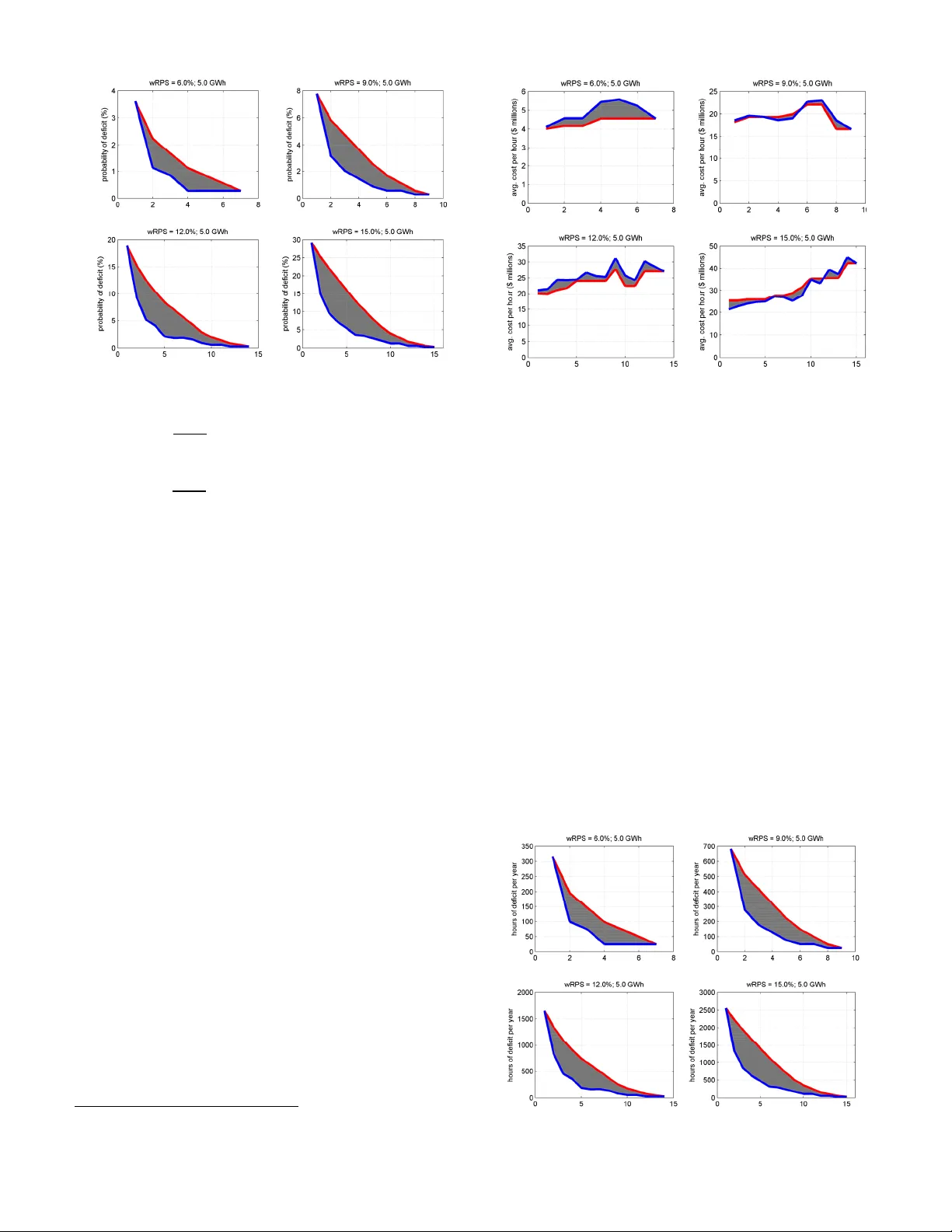
1  Abstract --As compared to load demand, frequent wind ene rgy intermittencies p roduce large short-term ( sub 1-hr to 3-hr) deficits (and surpluses) in the energy supply. These intermittent deficits pose systemic and str uctural risks that w ill likely lead to energy deficits that have signific ant reliability implications for energy syst em operators and cons umers. This work provides a toolset to help policy makers quant ify these first-order ris ks. The thinking method ology / framework shows that increasing wind energy penetration significantly incr eases the risk of loss in California. In addition, the work presents holistic risk tab les as a general innovation to help decision makers quickly grasp the full impact of risk. Index Terms --California, renewable energy, risk an alysis, systems enginee ring, wind po wer generation . I. I NTRODUCTION HIS work is presented as a companion to our paper submitted for publication [1]. Two important outputs in that report ar e: (1) If the com ponents in Cal ifornia’s Renewable Port folio Standar d (R PS) grow at current rates, wind energy will constitute 15% o f the state’s energy generation by 2016; 1 (2) The state has energy reserve capacity between 2 an d 5 GWh (5 t o 10% of total 20 09 energy demand) co nsisting of spinning (a nd other) reserves. For t he wind component of the RPS (wRPS) greater th an 5%, the current reserve capacity is too low a nd not corre ctly configured to mitigate the risks associated with wind intermittency. The random, frequ ent (hour-to -hour) an d large chan ges in wind energy output create deficits (and surpluses) (Fi g. 1) that impose new st resses and risks for the stability of the electric grid infrastructure. Without utili ty-scale energy storage assets, the nature of these risks is significantly d ifferent from other conventional energy sources li ke fossil fuels. Wind energy intermittencies cr eate systemic and structural risks. In this context, “systemic risk” d efines risk that is tied to the hour-to-h our operation o f the energ y grid. This type of risk affects the entire grid or major segments of it on a dynamic basis. St ructural risk is that associ ated with chronic shortfalls due to insufficient energy generation. This is a Financial support for this work is provided by GridByte, Inc. , Energy Policy Analytics Practice. S. O. George and H. B. George, Ph.D. are with GridByte, Inc., 65 Enterprise, Aliso Viejo, CA 92656 USA (e-mail: info@gridbyte.com). S. V. Nguyen, Ph.D. is with Shell Projects and Technology, Innovation and R&D Division, Houston, TX 77002 USA. 1 The quantity of 15% by 2016 is an illustrative benchmark from the data extrapolation presented in [1]. strategic plann ing problem that may stem from current use of simplistic macro-exchan ge equations in wh ich annu alized average energy from wRPS sources is made equivalent to energy produc ed from other no n-renewable sources. Since t he state does not plan to install redundant no n-renewable generating equipment to compensate for th e intermittencies of wind energy, the systemic / structural risks will rise as the fraction of wRPS increases. In this scenario, beyond about 5% wind penet ration [1] t he st ate m ay experience risks leading to losses of tens of billion s of dollars. In this wor k, the focus of wi nd energy risk pl anning is energy stability—not safety, as is more common in nuclear energy. Under normal condit ions (i.e., no storm or excessi ve load demand), it is not possible to forecast wind energy output with a high degree of confidence . As shown with the application of the hour-to-h our auto-correlation fun ction (hhACF) in [1], wind energy has large short-term predictive uncertainty. These, coupled with th e fact that wind energy generation may fall to zero, are the basic factors of energy instability represented by wind. This work provides a toolset for policy makers struggling to make the right energy p olicy choices that w ill have profound multi-decades im pact. In ou r view, proactive RPS energy policy choic es must be balanced wi th appropriat e understanding and mitigation of systemic and stru ctural risk. The consequence of inadequate risk strategies possi bly exposes the state to energy de fi cit crises in 6 to 10 years. Why should Californians take th is seriously? There is precedence of energy instability in our recent past; in the Risk Quantification Associated with W ind Ener gy Intermittency in California Sam O. George, Member, IEEE , H. Bola George, Ph.D. and Scott V. Nguyen, Ph.D. T Fig. 1: wRPS = 15% energy production and load demand profiles vs. hour for a scenario containing 15 contiguous days. No energy is produced when wind speed falls below 4 m/s or exceeds 25 m/s. In this case, no energy is produced in 26 (7.22%) out of 360 h ours. 2 structural energy crises of 2 000-2001, it is estimated that Californi a lost $40 to $45 bi llion (about 3.5% of Gross St ate Product (GSP)) [2]. During th is period, the state experienced rolling blackouts (load shedd ing) over 38 days [3] as energ y demand exceeded s upply by an average of 60 0 MW. In som e cases, electricity customers lo st power for up to 16 hours. 2 Again, as cited in [1], nota ble recent precedents e xist in Denmark an d Texas. A note about reading this document : The purpose is t o provide an analytics fra mework fo r energy risk quantification. Of course, it is possible that busin esses and government will not stand by and allow wRPS risks to becom e chronic. The reality is that we are operating under mandates codified in Californi a law (CA AB 32 / Gove rnor’s e xecutive order ) to achieve 33% RPS (R PS33) by 2030 . The logical action is that risk mitigation infrastructure will b e added to cope with the inherent intermittencies of wind energy. One essential component of risk m itigation infrastructure m ay include utility-scale storage. II. W IND E NERGY R ISK A NALYTICS A. The Faulty Energy-Exchange Macro Equation Without significant u tility-scale storage, wind en ergy should not be equated with ener gy from conve ntional sou rces (e.g., fossil- based). The underlying ri sk is that win d energy has large ra ndom short-te rm (sub 1-hr to 3-hr) intermittencies, as shown in Fig. 1, that necess itate constant com pensation [1]. The energy-exchange macro equati ons equate the statistical average energy from wRPS genera tor sites to the absolu te energy produced from conventi onal sources. Moreover, the statistical averages are often de rive d from dat a measured i n annual terms. This type of averag ing masks the short-term intermittencies that are important for grid stability. So, effectively, there are two or m ore 3 levels of averaging that lead to a faulty outcome. Wind energy dispatch is a r eal-time schedul ing problem . 1 GWh of energy from a fossil fired plant  1 GWh of ene rgy from any wind farm (or collecti on of wi nd farms). To m ake the macro energy -exchange equatio n “work” today, C alifornia relies on interruptible po wer agreements with large energy consumers [4] —this so-calle d demand-side compensatio n, is another ma jor element of risk. As shown by the precede nce of California’s 2000-2001 energy cris es, large businesses that use these interruptible power contr acts are m uch less tolerant of blackouts. During the energy cr ises, as exemplified by Fruit Growers Supp ly Co., a number of companies either sought to extricate themselves from thes e contracts [5] (see Section II- G) or chose t o keep power flowing at expe nsive premium rates. If we use precede nce as a guide, then the reliance on 2 Granted, the causes of the 2000-2001 energy crises stem from the implem entation of California’s electri city industry deregulation efforts—a scenario that is different from wRPS im plementation. However, the crises of 2000-2001 are instructive in the sim ple point that they should not have happened. If these crises fell outside the pr ojected normative behavior—then their occurrence i s instructive for wRPS implementation as it shows that outlier events can and will occur with se rious consequences. But importantly, the hour-to-hour system ic risk may become the norm ative as wRPS penetration increases. 3 There is one implicit level of averag ing in that reported wind speeds are averages derived from Weibull probability plots / analyses. interruptible power contract s poses a serious ris k to grid stability. B. Definition of Risk as use d in this w ork Formally, risk, R $ , is the pr oduct of tw o com ponents: (The probability of an Energy Deficit, P E Deficit )  (The Impact of Energy Deficits, I E Deficit ). R $ = P E Deficit  I E Deficit (1) It is our goal to present solu tions that comply with equation (1). When not possible, we will use a set of heuristics that follow the spirit of the equation. C. Definition o f Energy Deficit Measured on a short-term basis (sub 1-hr to 3-hr), energy deficit ( E Deficit ) is the dif ference bet ween dem and load ( E Demand ) and wRPS gene ration out put ( E wRPS ) + some reserve capacity ( E ResCap ). E Deficit = E Demand - E wRPS + E ResCap (2) We assume that the 2 to 5 G Wh spinning, and other, reserves can produce the fast response [1] required to compensate for the short-term intermittencies in wind energy output. Implicit in this assumption is the req uirement that the fast compensation rese rves must have non-stochastic real -time stability as compared to E wRPS output. D. Risk Factors While we restrict our disc ussi on to the first-order risk associated with energy deficits, it is important to note th at the dynamics of wR PS integration create a n umber of additi onal and significa nt risk factors. Table 1 presents a pa rtial summary of risk factors t hat ar e considered in the context of this work. E. Probability o f n-hr Deficit Clusters wRPS profiles , such as in Fig. 1, cont ain n -hr “natural” clusters of energ y deficit, i.e., contiguou s hour-to-hour deficits. The cluster lengths m ay be one or multiple hours long. For example, from Fig. 1, the “natural” formation produces clust ers ranging i n length fr om 1 hour to 15 h ours. While natural clusters are good for descrip tion of the experime ntal data, they pose a chall enge for form ing reliable probability metrics. Specifically, it is difficult to talk systematically about the prob ability of “naturally” formed clusters of different sizes. In the models for this work, we use “synthetic” clustering. We use two diffe rent counting m ethods that boun d the range of probabilities of synthetic n -hr cluster sizes. These synthetic clusters are deliberate constructs to ensure that th e probability computations y ield consist ent results. Application of these probability co unting methods (descr ibed in Section II-F ) produces probabilities for synthetic n -hr windo ws; i.e., 1 hr, 2 hr, 3 hr, ... etc. The im portant p oint is that the probabilities associated with the synthetic n -hr clusters exist orthogon ally; i.e., they can all be co mbined in the same space without affecting the accuracy of t he overall probability estimate. The or thogonal properties allow 3 application o f differe nt cost im pact factors as discussed in Section II-G . Fig. 2 present s a sample ap plication of t he synthetic de ficit cluster probability algo rithm (SDCPA) described in Section II- F . In this example, we utilize the wind energy generation scenario shown in Fig. 1 as the basis. The reserve capacit y of 5 GWh is assume d to be readily dispatchable to com pensate for any / all wind intermittencies. F. Synthetic deficit cluster probability algo rithm (SDCPA) This section presents the synthetic deficit cl uster probability algorithm (SDCPA). The algorithm is presented in ps eudo- code for simpli city. The SDCPA use s two met hods to calculate the probability of energy deficit clusters. Method 0 counts all non-over lapping n -hr synthetic ener gy deficit clusters. This method prod uces a slight unde rcounting as cluster sizes increase. Method 1 c ounts overlappi ng n -hr synthetic clust ers. This method p roduces a slight over-count. The SDCPA is implemented as follows: //Let ... e Demand = vector  energy dem and profil e by hour e wRPS = vector  wRPS energy pr oduction profi le by hour e De f ici t = vector  containing ener gy deficits v = vector  binary thres holds c 0  representing clusters (method 0 ) c 1 = vector  representing clusters (method 1 ) E R esCa p = scalar  total reserve capacity in grid N = scalar  number of ho urs in e Demand and e wRPS profiles h = scalar  subscript f or hour i = scalar  subscript for clusters n 0 = vector  Total number of cluster s and non- clusters; m ethod 0 n 1 = vector  Total number of cluster s and non- clusters; m ethod 1 p 0 = vector  probability of clusters; method 0 p 1 = vector  probability of clusters, method 1 //Create deficit vector ... For ( h = 1 to N, h ++ ) { e Deficit [ h ] = ( e Demand [ h ] – e wRPS [ h ] – E ResCap )  [( e Demand [ h ] – e wRPS [ h ]) ≥ 0]; v [ h ] = e Deficit [ h ] > 0; // v [ h ] is a 1D vector of 0’s or 1’s } // Create cluster vectors (met hod 0 and me thod 1) ... For ( i = 1 to 23; i ++) { // step size is always 1 For ( h = i to N; h++ ) { r = h – i +1;   󰇟  󰇠    󰇟󰇠    ; n 0 [ i ]++; } m = 0; For ( h = i to N; h + m ) { // step size is 1 or i q = h – i +1;   󰇟  󰇠    󰇟j󰇠    ;      󰇟j 󰇠    ; if ( m == 0, m = 1) n 1 [ i ]++; } // Calculate probabilities ... Table 1: wRPS Risk Factors Matrix Risk Factor Primary Risk Factors Notes 1 Large-magnitude hour-to-hour intermittencies i n wind energy generation capacity. With the state’s current reserve capacity a nd be yond 5% wind penetration [1], the large intermittencies of wind energy may lead to deficits of unpredictable magnitude and duration. 2 Rate of change of wind energ y generation output. Large hour-to-hour changes in wind energ y generation create ra mp-rate problems. Because it is difficult to predict the short-t erm output of wind farms in the grid , it may not be possible to deliver compensation energ y to grid-segments when required. The ram p- rate problem requires fast-res ponse generators to compensate for sudden changes in wind energy output. From Fig. 1, there ar e seve ral instances in which the hour-to-hour wind energy output varies by more than 10 GW. Fo r example, a 10 G W deficit requires the fast compensation generators to produce a sustai ned ~167 MW/min. Ramp-rates of this order are difficult to sustain with the mix of genera ting assets currently deplo yed in California. In our estimate, s uch a ramp rate requir e s tens of fast compensation gener ators. 3 Random periods of wind energy deficits and surpluses. Random intervals between wind energy deficits / surpluses. The length of time ass ociated with wind energy deficits (or sur pluses) is random. This produces large-scale planning uncertainty for grid operators. If these deficits translate to blackouts, the effects on the economy would ma gnify non-linearly. For ex ample, the grid operators may need to m aintain compensation generators in sub-optimal standby mode for many more hours than required. This prac ti ce constitutes a large l oss of revenue. 4 Transmission constraints. Compensating for wind energy defi c its is constrained by the tra nsmission infrastructure. Even if all the c ompensating generation capa city is dispatchable, there is a real possibilit y that the energy m ay not get to the c lients because of transm ission bottlenecks. 5. Rate of Implementation of wRPS. Evolution of the current grid follows an innov ation trajectory spanning 100 to 150 years. Most utility-sca le wRPS implementa tion experience is less than 2 0 year. Th e lack of field and technical ex perience / data constitutes an elem ent of risk. 4 Fig. 4: Summation of total number of hours corresponding to each n-hr cluster of energy deficits vs. n -hr clusters. The reserve capacity is 5 GWh.   󰇟  󰇠    󰇟  󰇠   󰇟  󰇠 ;   󰇟  󰇠    󰇟  󰇠   󰇟  󰇠 ; 󰇞 G. Impact of n-hr Wind Energy Defi cits The second co mponent of risk (eq. 1 ) is the dolla r-impact ( I E Deficit ) associated with n -hr energy deficits. Impact is the product of the normal ized loss-per- hour ( L hr ) and the total number of hours in the corresp onding n -hr deficit clusters ( N n- hr ). I E Deficit = L hr  N n-hr (3) Growth in the fraction of e nergy from wRPS means that most of Cal ifornia’s highly i nterconnected econom y will be adversely affected by energy deficits resulting from wind intermittencies. Thus we calibrate L hr based on broa d application of the sect or custom er damage functions (SC DF) developed i n [6]. L hr is based on the weighted average cost of 1-hour energy interrupti on for all sectors of the ec onomy. L hr uses a loss basis of $8.76 / kWh in 1996 dollars for the entire United States. In this work, our illustratio ns are computed with the 1996 l oss basis of $8.76 / k Wh. 4 As noted in [6][7], the economic losses associated with multi-hour deficits is non- linear, in that the “interruption costs increase with duration in a non-linear m anner.” Further, t he random and large intermittencies of wRPS generation complicate the calculations. To simplify our models, we apply the 1-h our loss-basis linearly across all clusters of deficits. Th us, the cost of larger deficit clusters are underestimates. Let us posit that California’s Gro ss State Product (GSP) is at parity when there is energy stability; i.e., d emand is equal to generation on an h our-to-hour basis. Parity means that t he grid, based on data for the en tire United States, can supply, 4 If we correct for inflation and other economic factors, the loss-basis is about $16.08 / kWh in 2009 dollars. The estimates in [6] represent a com prehensive loss basis from which other estimates can easily be drawn. 100% ener gy with a reliabil ity of 9 9.96% (cor respondin g to the highest reliability of 3.5 hours of blackouts per year) [6]. Using L hr and the SDCPA in Section II-F , the model computes the 1-hour dollar-impact as s hown in Fig. 3. For example, Fi g. 3 shows L hr at four wRPS penetration levels vs. synt hetic cluster sizes base d on a reserve ca pacity of 5 GWh. At wRPS = 15%, the L hr hour ranges from $21.38 million t o $43.32 milli on/hr. From application of the synthetic deficit cluster probability algorithm in Section II-F , we obt ain the total number of hours corresponding to each n -hr cluster show n in Fig. 4. For perspective, it is useful to review the dollar-impact o f energy defici ts during the 2000-2001 e nergy crises o n one California far ming operat ion [5][8]. As s hown, losses m ount and multiply qu ickly during multi-hour blackouts. As furth er illustrated in [7], the losses are often und er-reported. Businesses generall y have low tolerance f or blackouts—t hey quickly begin to inv est in blackout mitigation equ ipment (e.g., backup generators ). These investm ents are non-incremental business-continu ity insurance expend itures that, in addition to maintenance, re present loss of p rofit. The experi ence of the Fig. 2: Probability of ener gy deficits at different wRPS penetration levels with 5 GWh reserve capacity vs. n -hr deficit clusters in both overlap (red curve) and non-overlap (blue) form ulations. Fig. 3: Dollar-impact ( L hr ) of energy deficits at different wRPS penetration levels with 5 GWh reserve capacity vs. n -hr deficit-clusters. L hr is based on a loss-basis of $8.76 / kWh. 5 Fig. 6: Energy-supply reliability vs . wRPS penetration levels for t he generation / demand profiles shown in Fig. 1. At wRPS = 15% and reserve capacity = 5 GWh, th e reli ability drops to 70.83%. Land O’Lakes cooperative also illu strates that reliance on interruptible power con tracts is not workable if the en ergy deficits become frequent. Thus, the fact that large businesses sign up for interruptib le power programs should not be regarded as an indication of high risk tolerance. Rather, it is an exercise in busi ness operating-c ost minimi zation because these programs offer significan t discounts for particip ation. H. Risk Associated with Energy Deficits As defined in eq. 1 ( Section II -B ), the annualized Risk is the product of the probab ility of deficits ( Section II-E ) and the dollar-impact of these deficits ( Section II-G ). Building on the examples in these sections, we prese nt Fig. 5—a view of the risk associated with synthetic clus ters of en ergy deficits. Fi g. 5 shows ho w risk grows with increasing wRPS penet ration. To present a holistic view of risk , we show two snapshots of risk tabl es in Section II-J . I. How wRPS intermittency reduces Reliability To the first order, the risk posed b y wRPS intermittencies changes California’s reliability expectation s significantly. Reliability is one minus th e probability of en ergy deficits. At wRPS = 15% and reser ve capacity of 5 GWh, C alifornia’s energy generation reliability may dr op to 70.83%. Th is, as compared to nom inal baselin e performance of 99.96%, represents many hund red hours of energy d eficits. Fig. 6 presents the reliability profile vs. wRPS penetration lev els for the generatio n / dema nd profiles in Fi g. 1 for 1-hou r deficits . Beyond the first order, there are hi gher order risks associated with the frequency of energy deficits; i.e., in the wRPS scenario, the defici ts occur more fre quently and randomly. The associated loss of such instability is largely unknown, but potentially as large as th e first order risk presented in this work. J. Risk Tables—A classical view To present a com prehensi ve view of risk, t his section utilizes a classical method similar to that from the actuarial sciences. The underl ying equations are generally unwi eldy— thus the tabular format is more accessible. In this section we present two ex amples in Ta ble 2 (wRPS = 6%) and Ta ble 3 (wRPS = 15% ). From Tabl e 2, Cali fornia’s g rid can ‘sust ain’ wRPS = 6% with 5 GWh reserve capacity to produce associated risk between 0 and $1 billion . In contrast, Table 3 shows that the risk associat ed with wRPS= 15% exceeds $50 billion at a reserve cap acity of 5 GWh (10% of peak demand). The risk profile is much less fo r a reserve capacity of 10 GWh (20% of pea k demand)—b ut as discusse d in Section II I, California has t o re-evaluate the opport unity cost of wRPS vs. deploym ent of 10 GWh reserve capacity. III. Conclusion / Solutions In addition to th e conclusions in [1], th is work shows how / why risk quantification analytics methodology should be included in Ca lifornia’s wi nd RPS strategy. The ri sk tables in this work provide a holistic in sight into the probable losses associated with vari ous wRPS penetrat ion levels and res erve capacities. The loss-basis shown is con servative. This is further calibrated against estimated losses from California’s 2000-200 1 energy c rises. U sin g this loss-basis, we estim ate that Califo rnia’s risk ex posure in a wRPS = 15% s cenario could exceed tens of b illions per year in 2009 dollars. There is no easy way out—at high wRPS penetration levels (e.g., 15%) a significant fraction of the state’s GSP [9] will be lost directly from wRPS intermittency. If not directly, the loss in GSP will be felt indirectly as non-incremental expenditures are diverted to wRPS intermittency risk mitigation. Fig. 5: Conservative annualized risk vs. n -hr deficit cluster sizes for the state of California at various wRP S penetration levels. The reserve capacity is 5 GWh. 6 With a holistic view of risk, the state needs to re-evaluate the opportunity costs associated with wRPS implementation. For example, one way t o achieve wRPS = 15% is to invest in appropriate fast-response ener gy reserve capacity (such as combined-cycle gas-fired plants) or utility-scale stor age assets [1]. The state must also re-exa m ine whether reliance on interruptible power con tracts as a means for maintaining grid stability is workable in th e wRPS = 15% scenario. With the precedence of the 2000 -2001 crises coupled with these large risks, it is our view that interruptible power contracts are not workable as wRPS energy deficits increase in frequency, randomness and length. Table 2: Annualized Risk (in 2009 dollars ) at various wRPS = 6% penetration vs. n -hr energy deficit clust ers (The reserve capacities are 2 and 5 GWh) Method 1: Non-overlap met hod Method 0: Overlap Method wRPS (%) Reserve Capacity (GWh) n -hr Cluster Size (hours) Probability of n-hr Energy Deficit (%) Total Energy Deficit Hours per Year (hours) Total Energy Deficit P er Year (GWh) Economic Loss per Energy Deficit Hour ($MM) Risk per Year ($BB) Probability of n-hr Energy Deficit (%) Total Energy Deficit Hours per Year (hours) Total Energy Deficit P er Year (GWh) Economic Loss per Energy Deficit Hour ($MM) Risk per Year ($BB) 6 2 1 29.2 2556.8 68.36 8.55 21.860 29.2 2556.8 119.94 10.144 25.934 6 2 2 15.0 1316.3 65.94 9.149 12.043 25.3 2222 117.68 10.146 22.544 6 2 3 9.6 841.8 64.81 9.592 8.074 22.1 1934.4 117.54 10.334 19.990 6 2 4 7.1 619.8 62.26 9.872 6.119 19 1669.7 117.54 10.334 17.255 6 2 5 5.4 473.8 61.79 9.976 4.727 16 1403.5 117.54 10.334 14.504 6 2 6 3.6 316.2 58.73 10.865 3.435 13 1135.9 113.67 11.092 12.599 6 2 7 3.3 292.2 59.27 10.742 3.139 10.5 916.2 113.67 11.092 10.163 6 2 8 2.6 230.7 45.5 10.101 2.330 7.9 695.3 109.13 11.537 8.022 6 2 9 1.9 168.6 44.7 11.026 1.859 5.7 498.1 96.34 12.581 6.266 6 2 10 1.2 108.2 47.21 13.975 1.512 4 349.6 79.96 14.201 4.965 6 2 11 1.3 109.6 49.4 13.293 1.457 2.9 250.5 79.96 14.201 3.557 6 2 12 0.6 51.9 42.64 15.778 0.818 1.7 150.7 44.98 14.266 2.150 6 2 13 0.6 52.2 43.85 14.977 0.781 1.1 100.8 44.98 14.266 1.437 6 2 14 0.3 25.3 28.37 17.993 0.455 0.6 50.5 28.6 16.93 0.855 6 2 15 0.3 25.3 28.6 16.93 0.429 0.3 25.3 28.6 16.93 0.429 6 5 1 3.6 316.6 5.09 4.111 1.301 3.6 316.6 5.88 4.017 1.272 6 5 2 1.1 98.5 4.12 4.576 0.451 2.2 195.3 4.69 4.166 0.814 6 5 3 0.8 74.3 4.64 4.577 0.340 1.7 146.9 4.69 4.166 0.612 6 5 4 0.3 24.6 2.45 5.44 0.134 1.1 98.2 3.59 4.559 0.448 6 5 5 0.3 24.6 3.14 5.579 0.137 0.8 73.9 3.59 4.559 0.337 6 5 6 0.3 24.7 3.54 5.242 0.129 0.6 49.4 3.59 4.559 0.225 6 5 7 0.3 24.8 3.59 4.559 0.113 0.3 24.8 3.59 4.559 0.113 7 Table 3: Annualized Risk (in 2009 dollars ) at various wRPS = 15% penetration vs. n -hr energy deficit clusters (The reserve capacities are 2, 5 and 10 GWh) Method 1: Non-overlap met hod Method 0: Overlap Method wRPS (%) Reserve Capacity (GWh) n -hr Cluster Size (hours) Probability of n-hr Energy Deficit (%) Total Energy Deficit Hours per Year (hours) Total Energy Deficit P er Year (GWh) Economic Loss per Energy Deficit Hour ($MM) Risk per Year ($BB) Probability of n-hr Energy Deficit (%) Total Energy Deficit Hours per Year (hours) Total Energy Deficit P er Year (GWh) Economic Loss per Energy Deficit Hour ($MM) Risk per Year ($BB) 15 2 1 49.7 4358.6 440.48 35.239 153.593 49.7 4358.6 737.87 36.605 159.547 15 2 2 31.4 2751.4 435.32 36.469 100.339 45.1 3955.7 736.91 36.971 146.244 15 2 3 21.4 1878.4 415.43 37.263 69.996 41.1 3599.4 731.49 37.118 133.605 15 2 4 16.0 1406.9 394.08 38.037 53.514 37.3 3265.8 731.49 37.118 121.219 15 2 5 13.1 1151.5 404.58 37.817 43.545 33.4 2930.2 731.49 37.118 108.764 15 2 6 9.4 822.9 366.17 38.709 31.855 29.6 2592.8 727.22 37.986 98.490 15 2 7 7.7 677.0 383.82 40.575 27.471 26 2278.2 727.22 37.986 86.539 15 2 8 6.5 565.5 331.61 40.898 23.130 22.4 1961.8 715.81 38.996 76.503 15 2 9 5.1 445.1 315.56 38.919 17.325 19 1668.5 715.81 38.996 65.066 15 2 10 4.8 417.4 321.22 40.749 17.010 15.7 1373.6 715.81 38.996 53.565 15 2 11 4.4 385.7 321.89 43.309 16.704 12.3 1077 686.18 39.825 42.891 15 2 12 3.4 302.3 304.32 45.039 13.614 9.2 803.8 600.33 40.694 32.708 15 2 13 2.1 182.6 295.15 50.402 9.205 6.6 579.4 498.3 46.578 26.986 15 2 14 2.1 186.5 312.96 49.627 9.256 4.9 429.5 498.3 46.578 20.003 15 2 15 1.7 151.1 273.8 54.029 8.166 3.2 278.7 452.82 49.643 13.835 15 2 16 1.3 116.9 201.79 55.997 6.545 1.7 152.5 378.19 50.884 7.757 15 2 17 0.3 25.5 85.1 44.451 1.133 0.6 51 87.56 43.194 2.201 15 2 18 0.3 25.6 87.56 43.194 1.104 0.3 25.6 87.56 43.194 1.104 15 5 1 29.2 2556.8 170.91 21.375 54.651 29.2 2556.8 299.85 25.359 64.836 15 5 2 15.0 1316.3 164.85 22.874 30.109 25.3 2222 294.2 25.364 56.359 15 5 3 9.6 841.8 162.03 23.981 20.186 22.1 1934.4 293.84 25.835 49.974 15 5 4 7.1 619.8 155.65 24.681 15.298 19 1669.7 293.84 25.835 43.136 15 5 5 5.4 473.8 154.48 24.941 11.818 16 1403.5 293.84 25.835 36.260 15 5 6 3.6 316.2 146.83 27.163 8.588 13 1135.9 284.18 27.731 31.498 15 5 7 3.3 292.2 148.18 26.855 7.847 10.5 916.2 284.18 27.731 25.407 15 5 8 2.6 230.7 113.75 25.252 5.825 7.9 695.3 272.83 28.842 20.054 15 5 9 1.9 168.6 111.75 27.566 4.647 5.7 498.1 240.86 31.453 15.666 15 5 10 1.2 108.2 118.03 34.937 3.781 4 349.6 199.9 35.503 12.413 15 5 11 1.3 109.6 123.5 33.233 3.642 2.9 250.5 199.9 35.503 8.892 15 5 12 0.6 51.9 106.61 39.445 2.046 1.7 150.7 112.46 35.664 5.375 15 5 13 0.6 52.2 109.63 37.442 1.954 1.1 100.8 112.46 35.664 3.593 15 5 14 0.3 25.3 70.92 44.982 1.136 0.6 50.5 71.49 42.325 2.138 15 5 15 0.3 25.3 71.49 42.325 1.072 0.3 25.3 71.49 42.325 1.072 15 10 1 5.3 462.6 51.42 26.862 12.428 5.3 462.6 58.4 27.294 12.627 15 10 2 2.0 173.8 42.81 27.152 4.720 3.6 317.4 47.92 26.597 8.443 15 10 3 1.4 125.2 45.29 26.813 3.358 2.8 244.9 47.92 26.597 6.513 15 10 4 0.6 49.5 24.67 27.387 1.356 2 171.9 42.33 28.912 4.969 15 10 5 0.6 49.8 32.4 28.773 1.433 1.4 123.1 42.33 28.912 3.560 15 10 6 0.6 50.1 39.7 29.374 1.471 0.8 74.1 42.33 28.912 2.142 15 10 7 0.3 24.8 26.48 33.598 0.832 0.3 24.8 26.48 33.598 0.832 8 IV. R EFERENCES [1] S. O. George, H. B. George and S. V. Nguyen, “Effect of Wind Intermittency on the Electric Grid: Mitigating the Risk of Energy Deficits,” submitted to IEEE Tran sactions on Power Syste ms, December 2009. [2] C. Wea re, “The California Electricity Crisis: Causes and Policy Options,” Public Policy Ins titute of California, 2003. [3] Energy Information Agency ( EIA), “Subsequent Events-Califor nia’s Energy Crisis” [Online]. Available: http://eia.doe.gov/cneaf/electricity/ california/subsequentevents.htm l . [4] M. L. Wald, “Making Renewables Reliable,” The New York Tim es, November 18, 2009, [Online]. Available: http://www.nytimes.com /2009/11/19/business/businesss peci al2/19POWER.html?pagewanted=1 &_r=2&sq=matt%20wald%20wind&st=cse&scp=1 . [5] C. Merlo, “ California co-ops struggle to cope wit h the state's energy crisis,” Rur al Cooperatives Magazine, March/April 200 1 [Online]. Available: http://www.rurdev.usda.gov/ rbs/pub/mar01/peril.html . [6] P. J. Balducci, J. M. Roop, L. A. Schienbein, J. G. DeSteese and M. R. Weimar, “Electric al Power Interru p tion Cost Estimates for I ndividual Industries, Sectors, and U.S. Economy,” Pacific Nor thwest National Laboratory (PNNL) , Feb. 2002 [Online]. Available: http://www.pnl.g ov/main/publications/external/t echnical_r eports/pnnl-13797.pdf . [7] SENTECH, Inc., “2006 Update of Bu siness Downtim e Costs,” [Online]. Available: http://www.sentech.org/pdfs/2006%20Update%20of%20Bus iness%20Downtime%20Costs%20Final.pdf. [8] J. Lehrer and S. Micheals, “Energy Squeeze,” PBS Newshour, March 19, 2001 [Online] . Available: http://www.pbs.org/newshour/bb/econ omy/jan-june01/power_3-19. html. [9] Bureau of Econom ic Analysis (BEA), “Gross Domestic Product by State,” [Online]. Available: http://www.bea.gov/regional/gsp/ . V. B IOGRAPHIES Sam O. George (BS 1993) is an EE graduate of Iowa State University, Ames, Iowa. His competencies span a range of pr actices—high frequency / fidelity IC SoC product design / development (high frequency communications chipsets, power control subsystems and chipse ts, multi-loop tim ing recovery designs, e.g., Fractional-N PLLs, data converters, et. al), BIST, system s and software architecture / modeling, SaaS, computer algorithms, Intellectual Property monetization and business problem solving / BPO. Sam has led GridByte ® for the past seven years, a multi-practice consultancy that, am ong other things, pr oduces a range of risk-o ptimized strategic decision analytics tools / solutions f or corporate and government clients. This innovation to manage ment consulting combines engineering science and applied mathematics with systems expertise. In addition to consulting positions at a number of fortune 500 com panies, his career experience includes design management and IC lead positions at GlobespanVirata and Hughes Network Sy stems. In these positions he led high-frequency CMOS / BiCMOS chipse t designs and had direct design responsibility for RF / mixed-signal / analog sub-systems, systems architecture, device modeling, yield optim ization and DFM. H. Bola George (Ph.D. 2007) is an applied physics graduate of Harvard University. At GridByte, Inc., Bola has been focused on applying analytical frameworks to m odeling of real-time phy si cal systems, in particular, energy. Prior to employment at GridByte, Bola ’s work spanned investigation of surface mass transport mechanisms governing the fo rmation of nanoscale features, materials developm ent, a nd involvem ent with development of analytical tools to quantify morphological featur es. Scott V. Nguyen (Ph.D. 2006) is a Senior Physicist in Shell's Innovation and R&D division where he identifies and deve lops technology applicable to the sustainable development of unco nventional hydrocarbon re sources, focusing on techno-economics, energy m anagement , and greenhouse issues. He is a physics graduate of Harvard University and also currently ser ves on the advisory committee to the American Institute of Ph ysics Corporate Associates.