Introducing Monte Carlo Methods with R Solutions to Odd-Numbered Exercises

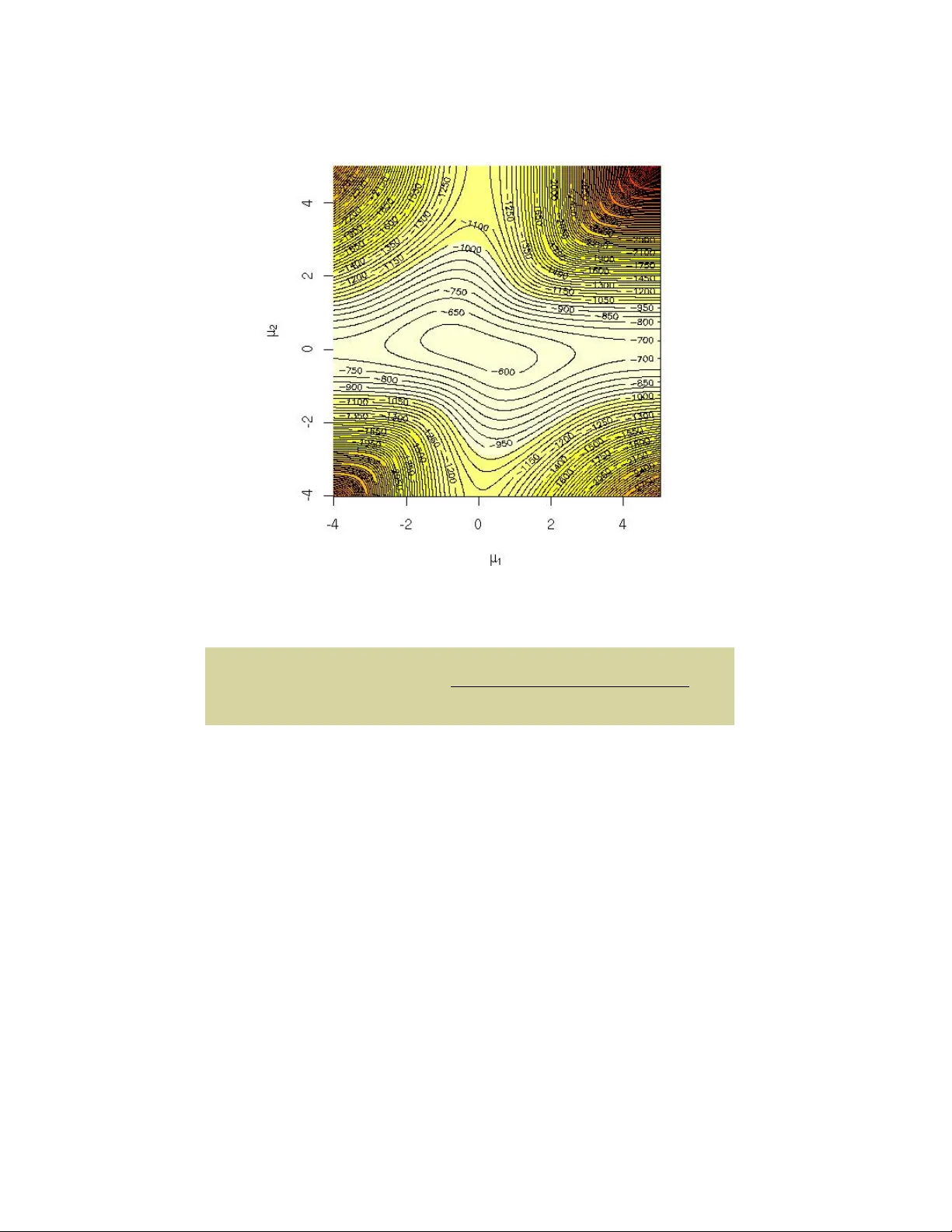
Christian Rob ert Univ ersit ´ e P aris-Dauphine and George Casella Univ ersit y of Florida In tro ducing Mon te Carlo Metho ds with R Solutions to Odd-Num b ered Exercises No vem ber 26, 2024 Preface The scrib es didn ’t have a lar ge enough set fr om which to determine p atterns. Brandon Sauderson The Her o of A ges This partial solution manual to our b o ok Intr o ducing Monte Carlo Metho ds with R , published by Springer V erlag in the User R! series, on December 2009, has b een compiled b oth from our own solutions and from homeworks written b y the following P aris-Dauphine students in the 2009-2010 Master in Statis- tical Information Pro cessing (TSI): Thomas Bredillet, Anne Sab ourin, and Jiazi T ang. Whenever appropriate, the R co de of those students has b een iden tiﬁed b y a # (C.) Name in the text. W e are grateful to those students for allo wing us to use their solutions. A few solutions in Chapter 4 are also taken verb atim from the solution manual to Monte Carlo Statistic al Metho ds com- piled by Roberto Casarin from the Universit y of Brescia (and only a v ailable to instructors from Springer V erlag). W e also incorporated in this manual indications ab out some typos found in the ﬁrst printing that came to our attention while comp osing this solu- tion manual hav e b een indicated as well. F ollo wing the new “print on de- mand” strategy of Springer V erlag, these typos will not b e found in the v ersions of the b o ok purchased in the coming months and should thus b e ignored. (Christian Rob ert’s b ook webpage at Universit ´ e P aris-Dauphine www.ceremade.dauphine.fr/~xian/books.html is a b etter reference for the “complete” list of typos.) Repro ducing the warning Jean-Mic hel Marin and Christian P . Rob ert wrote at the start of the solution manual to Bayesian Cor e , let us stress here that some self-study readers of Intr o ducing Monte Carlo Metho ds with R ma y come to the realisation that the solutions pro vided here are to o sketc hy for them b ecause the wa y we wrote those solutions assumes some minimal familiarit y with the maths, the probability theory and with the statistics b e- vi Preface hind the argumen ts. There is unfortunately a limit to the time and to the eﬀorts w e can put in this solution manual and studying Intr o ducing Monte Carlo Metho ds w ith R requires some prerequisites in maths (such as matrix algebra and Riemann in tegrals), in probability theory (suc h as the use of joint and conditional densities) and some bases of statistics (such as the notions of inference, suﬃciency and conﬁdence sets) that we cannot cov er here. Casella and Berger (2001) is a go od reference in case a reader is lost with the “basic” concepts or sk etch y math deriv ations. W e obviously welcome solutions, comments and questions on p ossibly er- roneous or ambiguous solutions, as well as suggestions for more elegant or more complete solutions: since this man ual is distributed both freely and in- dep enden tly from the b ook, it can be up dated and corrected [almost] in real time! Note how ev er that the R co des given in the follo wing pages are not opti- mised b ecause w e prefer to use simple and understandable co des, rather than condensed and eﬃcien t co des, b oth for time constrain ts and for p edagogical purp oses: some co des w ere written by our students. Therefore, if y ou ﬁnd b etter [meaning, more eﬃcient/faster] co des than those pro vided along those pages, w e w ould be glad to hear from y ou, but that do es not mean that we will automatically substitute your R co de for the curren t one, b ecause readability is also an imp ortan t factor. A ﬁnal request: this man ual comes in tw o versions, one corresponding to the o dd-num b ered exercises and freely a v ailable to ev eryone, and another one corresp onding to a larger collection of exercises and with restricted access to instructors only . Duplication and dissemination of the more extensiv e “in- structors only” version are obviously prohibited since, if the solutions to most exercises b ecome freely av ailable, the appeal of using our b o ok as a textbo ok will b e severely reduced. Therefore, if you happ en to p ossess an extended ver- sion of the manual, please refrain from distributing it and from repro ducing it. Sceaux and Gainesville Christian P . Rob ert and George Casella No vem b er 26, 2024 Con ten ts 1 Basic R programming . . . . . . . . . . . . . . . . . . . . . . . . . . . . . . . . . . . . . 1 Exercise 1.1 . . . . . . . . . . . . . . . . . . . . . . . . . . . . . . . . . . . . . . 1 Exercise 1.3 . . . . . . . . . . . . . . . . . . . . . . . . . . . . . . . . . . . . . . 1 Exercise 1.5 . . . . . . . . . . . . . . . . . . . . . . . . . . . . . . . . . . . . . . 1 Exercise 1.7 . . . . . . . . . . . . . . . . . . . . . . . . . . . . . . . . . . . . . . 2 Exercise 1.9 . . . . . . . . . . . . . . . . . . . . . . . . . . . . . . . . . . . . . . 2 Exercise 1.11 . . . . . . . . . . . . . . . . . . . . . . . . . . . . . . . . . . . . . 3 Exercise 1.13 . . . . . . . . . . . . . . . . . . . . . . . . . . . . . . . . . . . . . 3 Exercise 1.15 . . . . . . . . . . . . . . . . . . . . . . . . . . . . . . . . . . . . . 4 Exercise 1.17 . . . . . . . . . . . . . . . . . . . . . . . . . . . . . . . . . . . . . 4 Exercise 1.19 . . . . . . . . . . . . . . . . . . . . . . . . . . . . . . . . . . . . . 4 Exercise 1.21 . . . . . . . . . . . . . . . . . . . . . . . . . . . . . . . . . . . . . 4 Exercise 1.23 . . . . . . . . . . . . . . . . . . . . . . . . . . . . . . . . . . . . . 5 2 Random V ariable Generation . . . . . . . . . . . . . . . . . . . . . . . . . . . . . . 9 Exercise 2.1 . . . . . . . . . . . . . . . . . . . . . . . . . . . . . . . . . . . . . . 9 Exercise 2.3 . . . . . . . . . . . . . . . . . . . . . . . . . . . . . . . . . . . . . . 9 Exercise 2.5 . . . . . . . . . . . . . . . . . . . . . . . . . . . . . . . . . . . . . . 10 Exercise 2.7 . . . . . . . . . . . . . . . . . . . . . . . . . . . . . . . . . . . . . . 11 Exercise 2.9 . . . . . . . . . . . . . . . . . . . . . . . . . . . . . . . . . . . . . . 11 Exercise 2.11 . . . . . . . . . . . . . . . . . . . . . . . . . . . . . . . . . . . . . 11 Exercise 2.13 . . . . . . . . . . . . . . . . . . . . . . . . . . . . . . . . . . . . . 12 Exercise 2.15 . . . . . . . . . . . . . . . . . . . . . . . . . . . . . . . . . . . . . 13 Exercise 2.17 . . . . . . . . . . . . . . . . . . . . . . . . . . . . . . . . . . . . . 14 Exercise 2.19 . . . . . . . . . . . . . . . . . . . . . . . . . . . . . . . . . . . . . 15 Exercise 2.21 . . . . . . . . . . . . . . . . . . . . . . . . . . . . . . . . . . . . . 15 Exercise 2.23 . . . . . . . . . . . . . . . . . . . . . . . . . . . . . . . . . . . . . 16 3 Mon te Carlo Integration . . . . . . . . . . . . . . . . . . . . . . . . . . . . . . . . . . . 17 Exercise 3.1 . . . . . . . . . . . . . . . . . . . . . . . . . . . . . . . . . . . . . . 17 Exercise 3.3 . . . . . . . . . . . . . . . . . . . . . . . . . . . . . . . . . . . . . . 18 viii Con tents Exercise 3.5 . . . . . . . . . . . . . . . . . . . . . . . . . . . . . . . . . . . . . . 19 Exercise 3.7 . . . . . . . . . . . . . . . . . . . . . . . . . . . . . . . . . . . . . . 20 Exercise 3.9 . . . . . . . . . . . . . . . . . . . . . . . . . . . . . . . . . . . . . . 21 Exercise 3.11 . . . . . . . . . . . . . . . . . . . . . . . . . . . . . . . . . . . . . 22 Exercise 3.13 . . . . . . . . . . . . . . . . . . . . . . . . . . . . . . . . . . . . . 24 Exercise 3.15 . . . . . . . . . . . . . . . . . . . . . . . . . . . . . . . . . . . . . 24 Exercise 3.17 . . . . . . . . . . . . . . . . . . . . . . . . . . . . . . . . . . . . . 25 4 Con troling and Accelerating Conv ergence . . . . . . . . . . . . . . . . . . 27 Exercise 4.1 . . . . . . . . . . . . . . . . . . . . . . . . . . . . . . . . . . . . . . 27 Exercise 4.3 . . . . . . . . . . . . . . . . . . . . . . . . . . . . . . . . . . . . . . 27 Exercise 4.5 . . . . . . . . . . . . . . . . . . . . . . . . . . . . . . . . . . . . . . 28 Exercise 4.9 . . . . . . . . . . . . . . . . . . . . . . . . . . . . . . . . . . . . . . 28 Exercise 4.11 . . . . . . . . . . . . . . . . . . . . . . . . . . . . . . . . . . . . . 29 Exercise 4.13 . . . . . . . . . . . . . . . . . . . . . . . . . . . . . . . . . . . . . 29 Exercise 4.15 . . . . . . . . . . . . . . . . . . . . . . . . . . . . . . . . . . . . . 29 Exercise 4.17 . . . . . . . . . . . . . . . . . . . . . . . . . . . . . . . . . . . . . 30 Exercise 4.19 . . . . . . . . . . . . . . . . . . . . . . . . . . . . . . . . . . . . . 30 Exercise 4.21 . . . . . . . . . . . . . . . . . . . . . . . . . . . . . . . . . . . . . 32 5 Mon te Carlo Optimization . . . . . . . . . . . . . . . . . . . . . . . . . . . . . . . . . 35 Exercise 5.1 . . . . . . . . . . . . . . . . . . . . . . . . . . . . . . . . . . . . . . 35 Exercise 5.3 . . . . . . . . . . . . . . . . . . . . . . . . . . . . . . . . . . . . . . 35 Exercise 5.5 . . . . . . . . . . . . . . . . . . . . . . . . . . . . . . . . . . . . . . 36 Exercise 5.7 . . . . . . . . . . . . . . . . . . . . . . . . . . . . . . . . . . . . . . 37 Exercise 5.9 . . . . . . . . . . . . . . . . . . . . . . . . . . . . . . . . . . . . . . 39 Exercise 5.11 . . . . . . . . . . . . . . . . . . . . . . . . . . . . . . . . . . . . . 39 Exercise 5.13 . . . . . . . . . . . . . . . . . . . . . . . . . . . . . . . . . . . . . 40 Exercise 5.15 . . . . . . . . . . . . . . . . . . . . . . . . . . . . . . . . . . . . . 40 Exercise 5.17 . . . . . . . . . . . . . . . . . . . . . . . . . . . . . . . . . . . . . 42 Exercise 5.19 . . . . . . . . . . . . . . . . . . . . . . . . . . . . . . . . . . . . . 43 Exercise 5.21 . . . . . . . . . . . . . . . . . . . . . . . . . . . . . . . . . . . . . 43 6 Metrop olis-Hastings Algorithms . . . . . . . . . . . . . . . . . . . . . . . . . . . 45 Exercise 6.1 . . . . . . . . . . . . . . . . . . . . . . . . . . . . . . . . . . . . . . 45 Exercise 6.3 . . . . . . . . . . . . . . . . . . . . . . . . . . . . . . . . . . . . . . 45 Exercise 6.5 . . . . . . . . . . . . . . . . . . . . . . . . . . . . . . . . . . . . . . 46 Exercise 6.7 . . . . . . . . . . . . . . . . . . . . . . . . . . . . . . . . . . . . . . 46 Exercise 6.9 . . . . . . . . . . . . . . . . . . . . . . . . . . . . . . . . . . . . . . 47 Exercise 6.11 . . . . . . . . . . . . . . . . . . . . . . . . . . . . . . . . . . . . . 49 Exercise 6.13 . . . . . . . . . . . . . . . . . . . . . . . . . . . . . . . . . . . . . 50 Exercise 6.15 . . . . . . . . . . . . . . . . . . . . . . . . . . . . . . . . . . . . . 52 7 Gibbs Samplers . . . . . . . . . . . . . . . . . . . . . . . . . . . . . . . . . . . . . . . . . . . . 57 Exercise 7.1 . . . . . . . . . . . . . . . . . . . . . . . . . . . . . . . . . . . . . . 57 Con tents ix Exercise 7.5 . . . . . . . . . . . . . . . . . . . . . . . . . . . . . . . . . . . . . . 57 Exercise 7.7 . . . . . . . . . . . . . . . . . . . . . . . . . . . . . . . . . . . . . . 59 Exercise 7.9 . . . . . . . . . . . . . . . . . . . . . . . . . . . . . . . . . . . . . . 60 Exercise 7.11 . . . . . . . . . . . . . . . . . . . . . . . . . . . . . . . . . . . . . 61 Exercise 7.13 . . . . . . . . . . . . . . . . . . . . . . . . . . . . . . . . . . . . . 61 Exercise 7.15 . . . . . . . . . . . . . . . . . . . . . . . . . . . . . . . . . . . . . 62 Exercise 7.17 . . . . . . . . . . . . . . . . . . . . . . . . . . . . . . . . . . . . . 63 Exercise 7.19 . . . . . . . . . . . . . . . . . . . . . . . . . . . . . . . . . . . . . 64 Exercise 7.21 . . . . . . . . . . . . . . . . . . . . . . . . . . . . . . . . . . . . . 65 Exercise 7.23 . . . . . . . . . . . . . . . . . . . . . . . . . . . . . . . . . . . . . 65 Exercise 7.25 . . . . . . . . . . . . . . . . . . . . . . . . . . . . . . . . . . . . . 66 8 Con vergence Monitoring for MCMC Algorithms . . . . . . . . . . . 69 Exercise 8.1 . . . . . . . . . . . . . . . . . . . . . . . . . . . . . . . . . . . . . . 69 Exercise 8.3 . . . . . . . . . . . . . . . . . . . . . . . . . . . . . . . . . . . . . . 70 Exercise 8.5 . . . . . . . . . . . . . . . . . . . . . . . . . . . . . . . . . . . . . . 70 Exercise 8.7 . . . . . . . . . . . . . . . . . . . . . . . . . . . . . . . . . . . . . . 70 Exercise 8.9 . . . . . . . . . . . . . . . . . . . . . . . . . . . . . . . . . . . . . . 74 Exercise 8.11 . . . . . . . . . . . . . . . . . . . . . . . . . . . . . . . . . . . . . 76 Exercise 8.13 . . . . . . . . . . . . . . . . . . . . . . . . . . . . . . . . . . . . . 77 Exercise 8.15 . . . . . . . . . . . . . . . . . . . . . . . . . . . . . . . . . . . . . 77 Exercise 8.17 . . . . . . . . . . . . . . . . . . . . . . . . . . . . . . . . . . . . . 77 References . . . . . . . . . . . . . . . . . . . . . . . . . . . . . . . . . . . . . . . . . . . . . . . . . . . . . 79 1 Basic R programming Exercise 1.1 Self-explanatory . Exercise 1.3 Self-explanatory . Exercise 1.5 One problem is the w ay in whic h R handles paren theses. So > n=10 > 1:n pro duces 1 2 3 4 5 6 7 8 9 10 but > n=10 > 1:n-1 pro duces 0 1 2 3 4 5 6 7 8 9 since the 1:10 command is executed ﬁrst, then 1 is subtracted. The command seq(1,n-1,by=1) op erates just as 1:(n-1) . If n is less than 1 we can use something lik e seq(1,.05,by=-.01) . T ry it, and try some other v ariations. 2 1 Basic R programming Exercise 1.7 a. T o b o otstrap the data y ou can use the code Boot=2500 B=array(0,dim=c(nBoot, 1)) for (i in 1:nBoot){ ystar=sample(y,replace=T) B[i]=mean(ystar) } The quantile can b e estimated with sort(B)[.95*nBoot] , which in our case/sample is 5 . 8478. b. T o get a conﬁdence interv al requires a double b ootstrap. That is, for each b ootstrap sample w e can get a p oin t estimate of the 95% quantile. W e can then run an histogram on these quantiles with hist , and get their upp er and low er quantiles for a conﬁdence region. nBoot1=1000 nBoot2=1000 B1=array(0,dim=c(nBoot1, 1)) B2=array(0,dim=c(nBoot2, 1)) for (i in 1:nBoot1){ ystar=sample(y,replace=T) for (j in 1:nBoot2) B2[j]=mean(sample(ystar,replace=T)) B1[i]=sort(B2)[.95*nBoot2] } A 90% conﬁdence interv al is giv en b y > c(sort(B1)[.05*nBoot1], sort(B1)[.95*nBoot1]) [1] 4.731 6.844 or alternatively > quantile(B1,c(.05,.95)) 5% 95% 4.731 6.844 for the data in the b o ok. The command hist(B1) will give a histogram of the v alues. Exercise 1.9 If you type > mean function (x, ...) UseMethod("mean") 1 Basic R programming 3 y ou do not get any information ab out the function mean b ecause it is not written in R , while > sd function (x, na.rm = FALSE) { if (is.matrix(x)) apply(x, 2, sd, na.rm = na.rm) else if (is.vector(x)) sqrt(var(x, na.rm = na.rm)) else if (is.data.frame(x)) sapply(x, sd, na.rm = na.rm) else sqrt(var(as.vector(x), na.rm = na.rm)) } sho ws sd is written in R . The same applies to var and cov . Exercise 1.11 When lo oking at the description of attach , you can see that this command allo ws to use v ariables or functions that are in a database rather than in the curren t .RData . Those ob jects can b e temp orarily modiﬁed without altering their original format. (This is a fragile command that w e do not p ersonaly recommend!) The function assign is also rather fragile, but it allows for the creation and assignment of an arbitrary num b er of ob jects, as in the do cumen tation example: for(i in 1:6) { #-- Create objects ’r.1’, ’r.2’, ... ’r.6’ -- nam <- paste("r",i, sep=".") assign(nam, 1:i) } whic h allo ws to manipulate the r.1 , r.2 , ..., v ariables. Exercise 1.13 This is mostly self-explanatory . If y ou t yp e the help on eac h of those functions, y ou will see examples on how they work. The most recommended R function for saving R ob jects is save . Note that, when using write , the description states The data (usually a matrix) ’x’ are written to file ’file’. If ’x’ is a two-dimensional matrix you need to transpose it to get the columns in ’file’ the same as those in the internal representation. Note also that dump and sink are fairly inv olved and should use with caution. 4 1 Basic R programming Exercise 1.15 T ak e, for example a=3;x=c(1,2,3,4,5) to see that they are the same, and, in fact, are the same as max(which(x == a)) . F or y=c(3,4,5,6,7,8) , try match(x,y) and match(y,x) to see the diﬀerence. In contrast, x%in%y and y%in%y return true/false tests. Exercise 1.17 Running system.time on the three sets of commands give a. 0.004 0.000 0.071 b. 0 0 0 c. 0.000 0.000 0.001 and the v ectorial allocation is therefore the fastest. Exercise 1.19 The R co de is > A=matrix(runif(4),ncol=2) > A=A/apply(A,1,sum) > apply(A%*%A,1,sum) [1] 1 1 > B=A;for (t in 1:100) B=B%*%B > apply(B,1,sum) [1] Inf Inf and it shows that numerical inaccuracies in the pro duct leads to the prop ert y to fail when the pow er is high enough. Exercise 1.21 The function xyplot is part of the lattice library . Then > xyplot(age ~ circumference, data=Orange) > barchart(age ~ circumference, data=Orange) > bwplot(age ~ circumference, data=Orange) > dotplot(age ~ circumference, data=Orange) pro duce diﬀerent representations of the dataset. Fitting a linear mo del is simply done b y lm(age ~ circumference, data=Orange) and using the tree index as an extra co v ariate leads to 1 Basic R programming 5 >summary(lm(age ~ circumference+Tree, data=Orange)) Coefficients: Estimate Std. Error t value Pr(>|t|) (Intercept) -90.0596 55.5795 -1.620 0.116 circumference 8.7366 0.4354 20.066 < 2e-16 *** Tree.L -348.8982 54.9975 -6.344 6.23e-07 *** Tree.Q -22.0154 52.1881 -0.422 0.676 Tree.C 72.2267 52.3006 1.381 0.178 Tree^4 41.0233 52.2167 0.786 0.438 meaning that only Tree.L w as signiﬁcant. Exercise 1.23 a. A plain represen tation is > s [,1] [,2] [,3] [,4] [,5] [,6] [,7] [,8] [,9] [1,] 0 0 0 0 0 6 0 4 0 [2,] 2 7 9 0 0 0 0 5 0 [3,] 0 5 0 8 0 0 0 0 2 [4,] 0 0 2 6 0 0 0 0 0 [5,] 0 0 0 0 0 0 0 0 0 [6,] 0 0 1 0 9 0 6 7 3 [7,] 8 0 5 2 0 0 4 0 0 [8,] 3 0 0 0 0 0 0 8 5 [9,] 6 0 0 0 0 0 9 0 1 where empty slots are represen ted b y zeros. b. A simple cleaning of non-empt y (i.e. certain) slots is for (i in 1:9) for (j in 1:9){ if (s[i,j]>0) pool[i,j,-s[i,j]]=FALSE } c. In R , matrices (and arrays) are also considered as vectors. Hence s[i] represen ts the (1 + b ( i − 1) / 9 c , ( i − 1) mod 9 + 1) en try of the grid. d. This is self-explanatory . F or instance, > a=2;b=5 > boxa [1] 1 2 3 > boxb [1] 4 5 6 6 1 Basic R programming e. The ﬁrst lo op chec ks whether or not, for each remaining possible in teger, there exists an identical en try in the same row, in the same column or in the same b o x. The second command sets entries for whic h only one p ossible in teger remains to this integer. f. A plain R program solving the grid is while (sum(s==0)>0){ for (i in sample(1:81)){ if (s[i]==0){ a=((i-1)%%9)+1 b=trunc((i-1)/9)+1 boxa=3*trunc((a-1)/3)+1 boxa=boxa:(boxa+2) boxb=3*trunc((b-1)/3)+1 boxb=boxb:(boxb+2) for (u in (1:9)[pool[a,b,]]){ pool[a,b,u]=(sum(u==s[a,])+sum(u==s[,b]) +sum(u==s[boxa,boxb]))==0 } if (sum(pool[a,b,])==1){ s[i]=(1:9)[pool[a,b,]] } if (sum(pool[a,b,])==0){ print("wrong sudoku") break() } } } } and it stops with the outcome > s [,1] [,2] [,3] [,4] [,5] [,6] [,7] [,8] [,9] [1,] 1 3 8 5 2 6 7 4 9 [2,] 2 7 9 3 4 1 8 5 6 [3,] 4 5 6 8 7 9 3 1 2 [4,] 7 4 2 6 3 5 1 9 8 [5,] 9 6 3 1 8 7 5 2 4 [6,] 5 8 1 4 9 2 6 7 3 [7,] 8 9 5 2 1 3 4 6 7 [8,] 3 1 7 9 6 4 2 8 5 [9,] 6 2 4 7 5 8 9 3 1 1 Basic R programming 7 whic h is the solv ed Sudoku. 2 Random V ariable Generation Exercise 2.1 F or a random v ariable X with cdf F , if F − ( u ) = inf { x, F ( x ) ≤ u } , then, for U ∼ U [0 , 1], for all y ∈ R , P ( F − ( U ) ≤ y ) = P (inf { x, F ( x ) ≤ U } ≤ y ) = P ( F ( y ) ≥ U ) as F is non-decreasing = F ( y ) as U is uniform Exercise 2.3 a. It is easy to see that E [ U 1 ] = 0, and a standard calculation shows that v ar( U 1 ) = 1 / 12, from whic h the result follows. b. Histograms show that the tails of the 12 uniforms are not long enough. Consider the code nsim=10000 u1=runif(nsim) u2=runif(nsim) X1=sqrt(-2*log(u1))*cos(2*pi*u2) X2=sqrt(-2*log(u1))*sin(2*pi*u2) U=array(0,dim=c(nsim,1)) for(i in 1:nsim)U[i]=sum(runif(12,-.5,.5)) par(mfrow=c(1,2)) hist(X1) hist(U) a=3 mean(X1>a) mean(U>a) 10 2 Random V ariable Generation mean(rnorm(nsim)>a) 1-pnorm(a) c. Y ou should see the diﬀerence in the tails of the histogram. Also, the n u- merical output from the abov e is [1] 0.0016 [1] 5e-04 [1] 0.0013 [1] 0.001349898 where w e see that the Box-Muller and rnorm are very go o d when compared with the exact pnorm . T ry this calculation for a range of nsim and a . Exercise 2.5 F or U ∼ U [0 , 1] , Y ∼ g ( y ), and X ∼ f ( x ), such that f /g ≤ M , the acceptance condition in the Accept–Reject algorithm is that U ≤ f ( Y ) / ( M g ( Y )) . The probabilit y of acceptance is thus P ( U ≤ f ( Y )  M g ( Y )) = Z + ∞ −∞ Z f ( y M g ( y ) 0 d ug ( y ) d y = Z + ∞ −∞ f ( y ) M g ( y ) g ( y ) d y = 1 M Z + ∞ −∞ f ( y ) d y = 1 M . Assume f /g is only known up to a normalising constan t, i.e. f /g = k . ˜ f / ˜ g , with ˜ f / ˜ g ≤ ˜ M , ˜ M b eing a well-deﬁned upper b ound diﬀeren t from M b ecause of the missing normalising constan ts. Since Y ∼ g , P ( U ≤ ˜ f ( Y )  ˜ M ˜ g ( Y )) = Z + ∞ −∞ Z ˜ f ( y ˜ M ˜ g ( y ) 0 d ug ( y ) d y = Z + ∞ −∞ ˜ f ( y ) ˜ M ˜ g ( y ) g ( y ) d y = Z + ∞ −∞ f ( y ) k ˜ M g ( y ) g ( y ) d y = 1 k ˜ M . Therefore the missing constant is given by k = 1  ˜ M . P ( U ≤ ˜ f ( Y )  ˜ M ˜ g ( Y )) , whic h can b e estimated from the empirical acceptance rate. 2 Random V ariable Generation 11 Exercise 2.7 The ratio is equal to Γ ( α + β ) Γ ( α ) Γ ( β ) Γ ( a ) Γ ( b ) Γ ( a + b ) x α − a (1 − x ) β − b and it will not diverge at x = 0 only if a ≤ α and at x = 1 only if b ≤ β . The maxim um is attained for α − a x ? = β − b 1 − x ? , i.e. is M a,b = Γ ( α + β ) Γ ( α ) Γ ( β ) Γ ( a ) Γ ( b ) Γ ( a + b ) ( α − a ) α − a ( β − b ) β − b ( α − a + β − b ) α − a + β − b . The analytic study of this quantit y as a function of ( a, b ) is quite delicate but if we deﬁne mab=function(a,b){ lgamma(a)+lgamma(b)+(alph-a)*log(alph-a)+(beta-b)*log(beta-b) -(alph+bet-a-b)*log(alph+bet-a-b)} it is easy to see using contour on a sequence of a ’s and b ’s that the maximum of M a,b is achiev ed ov er in teger v alues when a = b α c and b = b β c . Exercise 2.9 Giv en θ , exiting the lo op is driven by X = x 0 , which indeed has a probability f ( x 0 | θ ) to occur. If X is a discrete random v ariable, this is truly a probability , while, if X is a contin uous random v ariable, this is zero. The distribution of the exiting θ is then dep enden t on the even t X = x 0 taking place, i.e. is prop ortional to π ( θ ) f ( x 0 | θ ), whic h is exactly π ( θ | x 0 ). Exercise 2.11 a. T ry the R co de nsim<-5000 n=25;p=.2; cp=pbinom(c(0:n),n,p) X=array(0,c(nsim,1)) for(i in 1:nsim){ u=runif(1) X[i]=sum(cp alpha) u=runif(1) U[i]=u } return(U) } Trans<-function(s0,alpha){ U=array(0,c(s0,1)) for (i in 1:s0) U[i]=alpha*runif(1) return(U) } Use hist(Wait(1000,.5)) and hist(Trans(1000,.5)) to see the corre- sp onding histograms. V ary n and α . Use the system.time command as in part a to see the timing. In particular, Wait is v ery bad if α is small. Exercise 2.13 The cdf of the P areto P ( α ) distribution is F ( x ) = 1 − x − α o ver (1 , ∞ ). Therefore, F − 1 ( U ) = (1 − U ) − 1 /α , which is also the − 1 /α p o wer of a uniform v ariate. 2 Random V ariable Generation 13 Exercise 2.15 Deﬁne the R functions Pois1<-function(s0,lam0){ spread=3*sqrt(lam0) t=round(seq(max(0,lam0-spread),lam0+spread,1)) prob=ppois(t,lam0) X=rep(0,s0) for (i in 1:s0){ u=runif(1) X[i]=max(t[1],0)+sum(prob nsim=100 > lambda=3.4 > system.time(Pois1(nsim,lambda)) user system elapsed 0.004 0.000 0.005 > system.time(Pois2(nsim,lambda)) user system elapsed 0.004 0.000 0.004 > system.time(rpois(nsim,lambda)) user system elapsed 0 0 0 for other v alues of nsim and lambda . Y ou will see that rpois is by far the b est, with the exp onen tial generator ( Pois2 ) not b eing very go od for large λ ’s. Note also that Pois1 is not appropriate for small λ ’s since it could then return negative v alues. 14 2 Random V ariable Generation Exercise 2.17 a. Since, if X ∼ G a ( α, β ), then β X = P α j =1 β X j ∼ G a ( α, 1), β is the inv erse of a scale parameter. b. The Accept-Reject ratio is giv en b y f ( x ) g ( x ) ∝ x n − 1 e − x λ e − λx = λ − 1 x n − 1 e − (1 − λ ) x . The maximum of this ratio is obtained for n − 1 x ? − (1 − λ ) = 0 , i.e. for x ? = n − 1 1 − λ . Therefore, M ∝ λ − 1  n − 1 1 − λ  n − 1 e − ( n − 1) and this upper bound is minimised in λ when λ = 1 /n . c. If g is the density of the G a ( a, b ) distribution and f the density of the G a ( α, 1) distribution, g ( x ) = x a − 1 e − bx b a Γ ( a ) and f ( x ) = x α − 1 e − x Γ ( α ) the Accept-Reject ratio is giv en by f ( x ) g ( x ) = x α − 1 e − x Γ ( a ) Γ ( α ) b a x a − 1 e − bx ∝ b − a x α − a e − x (1 − b ) . Therefore, ∂ ∂ x f g = b a e − x (1 − b ) x α − a − 1 { ( α − a ) − (1 − b ) x } pro vides x ? = α − a  1 − b as the argumen t of the maximum of the ratio, since f g (0) = 0. The upper b ound M is th us giv en b y M ( a, b ) = b − a  α − a 1 − b  α − a e − ( α − a 1 − b ) ∗ (1 − b ) = b − a  α − a (1 − b ) e  α − a . It obviously requires b < 1 and a < α . d. W arning: there is a typo in the text of the ﬁrst prin ting, it should b e: Sho w that the maximum of b − a (1 − b ) a − α is attained at b = a/α , and hence the optimal c hoice of b for sim ulating G a ( α, 1) is b = a/α , whic h giv es the same mean for b oth G a ( α, 1) and G a ( a, b ). 2 Random V ariable Generation 15 With this mo diﬁcation, the maxim um of M ( a, b ) in b is obtained by deriv a- tion, i.e. for b solution of a b − α − a 1 − b = 0 , whic h leads to b = a/α as the optimal choice of b . Both G a ( α, 1) and G a ( a, a/α ) ha ve the same mean α . e. Since M ( a, a/α ) = ( a/α ) − a  α − a (1 − a/α ) e  α − a = ( a/α ) − a α α − a = α α /a a , , M is decreasing in a and the largest possible v alue is indeed a = b α c . Exercise 2.19 The ratio f /g is f ( x ) g ( x ) = exp {− x 2 / 2 } / √ 2 π α exp {− α | x |} / 2 = p 2 /π α exp { α | x | − x 2 / 2 } and it is maximal when x = ± α , so M = p 2 /π exp { α 2 / 2 } /α . T aking the deriv ative in α leads to the equation α − 1 α 2 = 0 , that is, indeed, to α = 1. Exercise 2.21 W arning: There is a typo in this exercise, it should b e: (i). a mixture representation (2.2), where g ( x | y ) is the densit y of χ 2 p +2 y and p ( y ) is the densit y of P ( λ/ 2), and (ii). the sum of a χ 2 p − 1 random v ariable and the square of a N ( √ λ, 1). a. Show that b oth those representations hold. b. Compare the corresp onding algorithms that can b e derived from these represen tations among themselv es and also with rchisq for small and large v alues of λ . If we use the deﬁnition of the noncen tral chi squared distribution, χ 2 p ( λ ) as corresp onding to the distribution of the squared norm || x || 2 of a normal vector x ∼ N p ( θ , I p ) when λ = || θ || 2 , this distribution is in v ariant b y rotation ov er the normal vector and it is therefore the same as when x ∼ N p ((0 , . . . , 0 , √ λ ) , I p ), 16 2 Random V ariable Generation hence leading to the represen tation (ii), i.e. as a sum of a χ 2 p − 1 random v ariable and of the square of a N ( || θ || , 1) v ariable. Represen tation (i) holds b y a regular mathematical argument based on the series expansion of the mo diﬁed Bessel function since the density of a non-cen tral c hi-squared distribution is f ( x | λ ) = 1 2 ( x/λ ) ( p − 2) / 4 I ( p − 2) / 2 ( √ λx ) e − ( λ + x ) / 2 , where I ν ( t ) =  t 2  ν ∞ X k =0 ( z / 2) 2 k k ! Γ ( ν + k + 1) . Since rchisq includes an optional non-centralit y parameter nc , it can be used to simulate directly a noncentral chi-squared distribution. The t wo sce- narios (i) and (ii) lead to the follo wing R co des. > system.time({x=rchisq(10^6,df=5,ncp=3)}) user system elapsed > system.time({x=rchisq(10^6,df=4)+rnorm(10^6,mean=sqrt(3))^2}) user system elapsed 1.700 0.056 1.757 > system.time({x=rchisq(10^6,df=5+2*rpois(10^6,3/2))}) user system elapsed 1.168 0.048 1.221 Rep eated exp erimen ts with other v alues of p and λ lead to the same conclu- sion that the Poisson mixture representation is the fastest. Exercise 2.23 Since the ratio π ( θ | x ) /π ( θ ) is the likelihoo d, it is obvious that the optimal b ound M is the likelihoo d function ev aluated at the MLE (assuming π is a true density and not an improp er prior). Sim ulating from the posterior can then be done via theta0=3;n=100;N=10^4 x=rnorm(n)+theta0 lik=function(the){prod(dnorm(x,mean=the))} M=optimise(f=function(the){prod(dnorm(x,mean=the))}, int=range(x),max=T)$obj theta=rcauchy(N) res=(M*runif(N)>apply(as.matrix(theta),1,lik));print(sum(res)/N) while (sum(res)>0){le=sum(res);theta[res]=rcauchy(le) res[res]=(M*runif(le)>apply(as.matrix(theta[res]),1,lik))} The rejection rate is giv en by 0 . 9785, which means that the Cauc hy prop osal is quite ineﬃcien t. An empirical conﬁdence (or credible) in terv al at the lev el 95% on θ is (2 . 73 , 3 . 799). Rep eating the exp erimen t with n = 100 leads (after a while) to the in terv al (2 . 994 , 3 . 321), there is therefore an impro vemen t. 3 Mon te Carlo In tegration Exercise 3.1 a. The plot of the in tegrands follo ws from a simple R program: f1=function(t){ t/(1+t*t)*exp(-(x-t)^2/2)} f2=function(t){ 1/(1+t*t)*exp(-(x-t)^2/2)} plot(f1,-3,3,col=1,ylim=c(-0.5,1),xlab="t",ylab="",ty="l") plot(f2,-3,3,add=TRUE,col=2,ty="l") legend("topright", c("f1=t.f2","f2"), lty=1,col=1 :2) Both numerator and denominator are expectations under the Cauch y dis- tribution. They can therefore be appro ximated directly b y Niter=10^4 co=rcauchy(Niter) I=mean(co*dnorm(co,mean=x))/mean(dnorm(co,mean=x)) W e thus get > x=0 > mean(co*dnorm(co,mean=x))/mean(dnorm(co,mean=x)) [1] 0.01724 > x=2 > mean(co*dnorm(co,mean=x))/mean(dnorm(co,mean=x)) [1] 1.295652 > x=4 > mean(co*dnorm(co,mean=x))/mean(dnorm(co,mean=x)) [1] 3.107256 b. Plotting the con vergence of those in tegrands can b e done via # (C.) Anne Sabourin, 2009 x1=dnorm(co,mean=x) estint2=cumsum(x1)/(1:Niter) esterr2=sqrt(cumsum((x1-estint2)^2))/(1:Niter) 18 3 Monte Carlo Integration x1=co*x1 estint1=cumsum(x1))/(1:Niter) esterr2=sqrt(cumsum((x1-estint1)^2))/(1:Niter) par(mfrow=c(1,2)) plot(estint1,type="l",xlab="iteration",ylab="",col="gold") lines(estint1-2*esterr1,lty=2,lwd=2) lines(estint1+2*esterr1,lty=2,lwd=2) plot(estint2,type="l",xlab="iteration",ylab="",col="gold") lines(estint2-2*esterr2,lty=2,lwd=2) lines(estint2+2*esterr2,lty=2,lwd=2) Because we hav e not yet discussed the ev aluation of the error for a ratio of estimators, we consider b oth terms of the ratio separately . The empirical v ariances ˆ σ are giv en by var(co*dnorm(co,m=x)) and var(dnorm(co,m=x)) and solving 2 ˆ σ / √ n < 10 − 3 leads to an ev aluation of the n umber of simulations necessary to get 3 digits of accuracy . > x=0;max(4*var(dnorm(co,m=x))*10^6, + 4*var(co*dnorm(co,m=x))*10^6) [1] 97182.02 > x=2; 4*10^6*max(var(dnorm(co,m=x)),var(co*dnorm(co,m=x))) [1] 220778.1 > x=4; 10^6*4*max(var(dnorm(co,m=x)),var(co*dnorm(co,m=x))) [1] 306877.9 c. A similar implementation applies for the normal simulation, replacing dnorm with dcauchy in the ab o v e. The comparison is clear in that the required n umber of normal sim ulations when x = 4 is 1398 . 22, to compare with the abov e 306878. Exercise 3.3 Due to the identit y P ( X > 20) = Z ∞ 20 exp( − x 2 2 ) √ 2 π d x = Z 1 / 20 0 exp( − 1 2 ∗ u 2 ) 20 u 2 √ 2 π 20d u , w e can see this integral as an expe ctation under the U (0 , 1 / 20) distribution and th us use a Mon te Carlo approximation to P ( X > 20). The following R co de monitors the con vergence of the corresponding appro ximation. # (C.) Thomas Bredillet, 2009 h=function(x){ 1/(x^2*sqrt(2*pi)*exp(1/(2*x^2)))} par(mfrow=c(2,1)) curve(h,from=0,to=1/20,xlab="x",ylab="h(x)",lwd="2") I=1/20*h(runif(10^4)/20) estint=cumsum(I)/(1:10^4) esterr=sqrt(cumsum((I-estint)^2))/(1:10^4) 3 Monte Carlo Integration 19 plot(estint,xlab="Iterations",ty="l",lwd=2, ylim=mean(I)+20*c(-esterr[10^4],esterr[10^4]),ylab="") lines(estint+2*esterr,col="gold",lwd=2) lines(estint-2*esterr,col="gold",lwd=2) The estimated probability is 2 . 505 e − 89 with an error of ± 3 . 61 e − 90, compared with > integrate(h,0,1/20) 2.759158e-89 with absolute error < 5.4e-89 > pnorm(-20) [1] 2.753624e-89 Exercise 3.5 W arning: due to the (late) inclusion of an extra-exercise in the b ook, the “ab o v e exercise” actually means Exercise 3.3!!! When Z ∼ N (0 , 1), with density f , the quantit y of in terest is P ( Z > 4 . 5), i.e. E f [ I Z > 4 . 5 ]. When g is the density of the exponential E xp ( λ ) distribution truncated at 4 . 5, g ( y ) = 1 y > 4 . 5 λ exp( − λy ) R ∞ − 4 . 5 λ exp( − λy ) d y = λe − λ ( y − 4 . 5) I y > 4 . 5 , sim ulating iid Y ( i ) ’s from g is straightforw ard. Giv en that the indicator func- tion I Y > 4 . 5 is then alw ays equal to 1, P ( Z > 4 . 5) is estimated by ˆ h n = 1 n n X i =1 f ( Y ( i ) ) g ( Y ( i ) ) . A corresp onding estimator of its v ariance is v n = 1 n n X i =1 (1 − ˆ h n ) 2 f ( Y ( i ) )  g ( Y ( i ) ) . The follo wing R co de monitors the conv ergence of the estimator (with λ = 1 , 10) # (C.) Anne Sabourin, 2009 Nsim=5*10^4 x=rexp(Nsim) par(mfcol=c(1,3)) for (la in c(.5,5,50)){ y=(x/la)+4.5 weit=dnorm(y)/dexp(y-4.5,la) est=cumsum(weit)/(1:Nsim) 20 3 Monte Carlo Integration varest=cumsum((1-est)^2*weit/(1:Nsim)^2) plot(est,type="l",ylim=c(3e-6,4e-6),main="P(X>4.5) estimate", sub=paste("based on E(",la,") simulations",sep=""),xlab="",ylab="") abline(a=pnorm(-4.5),b=0,col="red") } When ev aluating the impact of λ on the v ariance (and hence on the conv er- gence) of the estimator, similar graphs can b e plotted for diﬀeren t v alues of λ . This exp erimen t does not exhibit a clear pattern, even though large v alues of λ , like λ = 20 app ear to slow down con vergence v ery m uch. Figure 3.1 sho ws the output of such a comparison. Picking λ = 5 seems ho wev er to produce a v ery stable approximation of the tail probability . Fig. 3.1. Comparison of three imp ortance sampling appro ximations to the normal tail probability P ( Z > 4 . 5) based on a truncated E xp ( λ ) distribution with λ = . 5 , 5 . 50. The straigh t red line is the true v alue. Exercise 3.7 While the exp ectation of p x/ (1 − x ) is well deﬁned for ν > 1 / 2, the integral of x/ (1 − x ) against the t density does not exist for an y ν . Using an importance 3 Monte Carlo Integration 21 sampling representation, Z x 1 − x f 2 ( x ) g ( x ) d x = ∞ if g (1) is ﬁnite. The in tegral will b e ﬁnite around 1 when 1 / (1 − t ) g ( t ) is in- tegrable, which means that g ( t ) can go to inﬁnit y at any rate. F or instance, if g ( t ) ≈ (1 − t ) − α around 1, an y α > 0 is acceptable. Exercise 3.9 As in Exercise 3.1, the quantit y of in terest is δ π ( x ) = E π ( θ | x ) = R θ π ( θ | x ) d θ where x ∼ N ( θ , 1) and θ ∼ C (0 , 1). The target distribution is π ( θ | x ) ∝ π ( θ ) e − ( x − θ ) 2 / 2 = f x ( θ ) . A p ossible imp ortance function is the prior distribution, g ( θ ) = 1 π (1 + θ 2 ) and for every θ ∈ R , f x ( θ ) g ( θ ) ≤ M , when M = π . Therefore, generating from the prior g and accepting simulations according to the Accept-Reject ratio pro vides a sample from π ( θ | x ). The empirical mean of this sample is then a con verging estimator of E π ( θ | x ) . F urthermore, we directly deduce the esti- mation error for δ . A graphical ev aluation of the conv ergence is given by the follo wing R program: f=function(t){ exp(-(t-3)^2/2)/(1+t^2)} M=pi Nsim=2500 postdist=rep(0,Nsim) for (i in 1:Nsim){ u=runif(1)*M postdist[i]=rcauchy(1) while(u>f(postdist[i])/dcauchy(postdist[i])){ u=runif(1)*M postdist[i]=rcauchy(1) }} estdelta=cumsum(postdist)/(1:Nsim) esterrd=sqrt(cumsum((postdist-estdelta)^2))/(1:Nsim) par(mfrow=c(1,2)) C1=matrix(c(estdelta,estdelta+2*esterrd,estdelta-2*esterrd),ncol=3) matplot(C1,ylim=c(1.5,3),type="l",xlab="Iterations",ylab="") plot(esterrd,type="l",xlab="Iterations",ylab="") 22 3 Monte Carlo Integration Exercise 3.11 a. If X ∼ E xp (1) then for x ≥ a , P [ a + X < x ] = Z x − a 0 exp( − t ) d t = Z x a exp( − t + a ) d t = P ( Y < x ) when Y ∼ E xp + ( a, 1), b. If X ∼ χ 2 3 , then P ( X > 25) = Z + ∞ 25 2 − 3 / 2 Γ ( 3 2 ) x 1 / 2 exp( − x/ 2) d x = Z + ∞ 12 . 5 p ( x ) exp( − 12 . 5) Γ ( 3 2 ) exp( − x + 12 . 5) d x . The corresp onding R co de # (C.) Thomas Bredilllet, 2009 h=function(x){ exp(-x)*sqrt(x)/gamma(3/2)} X = rexp(10^4,1) + 12.5 I=exp(-12.5)*sqrt(X)/gamma(3/2) estint=cumsum(I)/(1:10^4) esterr=sqrt(cumsum((I-estint)^2))/(1:10^4) plot(estint,xlab="Iterations",ty="l",lwd=2, ylim=mean(I)+20*c(-esterr[10^4],esterr[10^4]),ylab="") lines(estint+2*esterr,col="gold",lwd=2) lines(estint-2*esterr,col="gold",lwd=2) giv es an ev aluation of the probability as 1 . 543 e − 05 with a 10 − 8 error, to compare with > integrate(h,12.5,Inf) 1.544033e-05 with absolute error < 3.4e-06 > pchisq(25,3,low=F) [1] 1.544050e-05 Similarly , when X ∼ t 5 , then P ( X > 50) = Z ∞ 50 Γ (3) p (5 ∗ π ) Γ (2 , 5)(1 + t 2 5 ) 3 exp( − t + 50) exp( − t + 50) d t and a corresponding R co de # (C.) Thomas Bredilllet, 2009 h=function(x){ 1/sqrt(5*pi)*gamma(3)/gamma(2.5)*1/(1+x^2/5)^3} integrate(h,50,Inf) X = rexp(10^4,1) + 50 I=1/sqrt(5*pi)*gamma(3)/gamma(2.5)*1/(1+X^2/5)^3*1/exp(-X+50) 3 Monte Carlo Integration 23 estint=cumsum(I)/(1:10^4) esterr=sqrt(cumsum((I-estint)^2))/(1:10^4) plot(estint,xlab="Mean and error range",type="l",lwd=2, ylim=mean(I)+20*c(-esterr[10^4],esterr[10^4]),ylab="") lines(estint+2*esterr,col="gold",lwd=2) lines(estint-2*esterr,col="gold",lwd=2) As seen on the graph, this metho d induces jumps in the conv ergence patterns. Those jumps are indicative of v ariance problems, as should b e since the estimator do es not ha v e a ﬁnite v ariance in this case. The v alue returned by this approach diﬀers from alternatives ev aluations: > mean(I) [1] 1.529655e-08 > sd(I)/10^2 [1] 9.328338e-10 > integrate(h,50,Inf) 3.023564e-08 with absolute error < 2e-08 > pt(50,5,low=F) [1] 3.023879e-08 and cannot be trusted. c. W arning: There is a missing line in the text of this question, whic h should read: Explore the gain in eﬃciency from this metho d. T ak e a = 4 . 5 in part (a) and run an experiment to determine how man y normal N (0 , 1) random v ariables would b e needed to calculate P ( Z > 4 . 5) to the same accuracy obtained from using 100 random v ariables in this importance sampler. If we use the represen tation P ( Z > 4 . 5) = Z ∞ 4 . 5 ϕ ( z ) d z = Z ∞ 0 ϕ ( x + 4 . 5) exp( x ) exp( − x ) d x , the appro ximation based on 100 realisations from an E xp (1) distribution, x 1 m . . . , x 1 00, is 1 100 100 X i =1 ϕ ( x i + 4 . 5) exp( x i ) and the R co de > x=rexp(100) > mean(dnorm(x+4.5)*exp(x)) [1] 2.817864e-06 > var(dnorm(x+4.5)*exp(x))/100 [1] 1.544983e-13 24 3 Monte Carlo Integration sho ws that the v ariance of the resulting estimator is about 10 − 13 . A simple sim ulation of a normal sample of size m and the resulting accoun ting of the p ortion of the sample abov e 4 . 5 leads to a binomial estimator with a v ariance of P ( Z > 4 . 5) P ( Z < 4 . 5) /m , whic h results in a low er b ound m ≥ P ( Z > 4 . 5) P ( Z < 4 . 5) / 1 . 510 − 13 ≈ 0 . 7510 7 , i.e. close to ten million simulations. Exercise 3.13 F or the three choices, the imp ortance w eights are easily computed: x1=sample(c(-1,1),10^4,rep=T)*rexp(10^4) w1=exp(-sqrt(abs(x1)))*sin(x1)^2*(x1>0)/.5*dexp(x1) x2=rcauchy(10^4)*2 w2=exp(-sqrt(abs(x2)))*sin(x2)^2*(x2>0)/dcauchy(x2/2) x3=rnorm(10^4) w3=exp(-sqrt(abs(x3)))*sin(x3)^2*(x3>0)/dnorm(x3) They can be ev aluated in many w ays, from boxplot(as.data.frame(cbind(w1,w2,w3))) to computing the eﬀective sample size 1/sum((w1/sum(w1))^2) introduced in Example 3.10. The preferable choice is then g 1 . The estimated sizes are giv en b y > 4*10^6*var(x1*w1/sum(w1))/mean(x1*w1/sum(w1))^2 [1] 10332203 > 4*10^6*var(x2*w2/sum(w2))/mean(x2*w2/sum(w2))^2 [1] 43686697 > 4*10^6*var(x3*w3/sum(w3))/mean(x3*w3/sum(w3))^2 [1] 352952159 again sho wing the appeal of using the double exp onen tial proposal. (Note that eﬃciency could be doubled by considering the absolute v alues of the simula- tions.) Exercise 3.15 a. With a p ositiv e density g and the representation m ( x ) = Z Θ f ( x | θ ) π ( θ ) g ( θ ) g ( θ ) d θ , w e can simulate θ i ’s from g to approximate m ( x ) with 1 n n X i =1 f ( x | θ i ) π ( θ i ) g ( θ i ) . 3 Monte Carlo Integration 25 b. When g ( x ) = π ( θ | x ) = f ( x | θ ) π ( θ ) /K , then K 1 n n X i =1 f ( x | X i ) π ( X i ) f ( X i | θ ) π ( θ ) = K and the normalisation constant is the exact estimate. If the normalising constan t is unknown, we must use instead the self-normalising version (3.7). c. Since Z Θ τ ( θ ) f ( x | θ ) π ( θ ) π ( θ | x )d θ = Z Θ τ ( θ ) f ( x | θ ) π ( θ ) f ( x | θ ) π ( θ ) m ( x ) d θ = 1 m ( x ) , w e hav e an unbiased estimator of 1 /m ( x ) based on simulations from the p osterior, 1 T T X t =1 τ ( θ ∗ i ) f ( x | θ ∗ i ) π ( θ ∗ i ) and hence a con verging (if biased) estimator of m ( x ). This estimator of the marginal density can then b e seen as an harmonic mean estimator, but also as an imp ortance sampling estimator (Rob ert and Marin, 2010). Exercise 3.17 W arning: There is a typo in question b, which should read Let X | Y = y ∼ G (1 , y ) and Y ∼ E xp (1). a. If ( X i , Y i ) ∼ f X Y ( x, y ), the Strong La w of Large Numbers tells us that lim n 1 n n X i =1 f X Y ( x ∗ , y i ) w ( x i ) f X Y ( x i , y i ) = Z Z f X Y ( x ∗ , y ) w ( x ) f X Y ( x, y ) f X Y ( x, y )d x d y. No w cancel f X Y ( x, y ) and use that fact that R w ( x ) dx = 1 to show Z Z f X Y ( x ∗ , y ) w ( x ) f X Y ( x, y ) f X Y ( x, y )d x d y = Z f X Y ( x ∗ , y ) dy = f X ( x ∗ ) . b. The exact marginal is Z  y e − y x  e − y dy = Z y 2 − 1 e − y (1+ x ) dy = γ (2) (1 + x ) 2 . W e tried the following R v ersion of Monte Carlo marginalization: X=rep(0,nsim) Y=rep(0,nsim) for (i in 1:nsim){ 26 3 Monte Carlo Integration Y[i]=rexp(1) X[i]=rgamma(1,1,rate=Y[i]) } MCMarg=function(x,X,Y){ return(mean((dgamma(x,1,rate=Y)/dgamma(X,1, rate=Y))*dgamma(X,7,rate=3))) } True=function(x)(1+x)^(-2) whic h uses a G a (7 , 3) distribution to marginalize. It w orks ok, as you can c heck by looking at the plot > xplot=seq(0,5,.05);plot(xplot,MCMarg(xplot,X,Y)-True(xplot)) c. Cho osing w ( x ) = f X ( x ) leads to the estimator 1 n n X i =1 f X Y ( x ∗ , y i ) f X ( x i ) f X Y ( x i , y i ) = 1 n n X i =1 f X ( x ∗ ) f Y | X ( y i | x ∗ ) f X ( x i ) f X ( x i ) f Y | X ( y i | x i ) = f X ( x ∗ ) 1 n n X i =1 f Y | X ( y i | x ∗ ) f Y | X ( y i | x i ) whic h pro duces f X ( x ∗ ) mo dulo an estimate of 1. If we decomp ose the v ariance of the estimator in terms of v ar  E  f X Y ( x ∗ , y i ) w ( x i ) f X Y ( x i , y i )     x i  + E  v ar  f X Y ( x ∗ , y i ) w ( x i ) f X Y ( x i , y i )     x i  , the ﬁrst term is E  f X Y ( x ∗ , y i ) w ( x i ) f X Y ( x i , y i )     x i  = f X ( x ∗ ) E  f Y | X ( y i | x ∗ ) f Y | X ( y i | x i )     x i  w ( x i ) f X ( x i ) = f X ( x ∗ ) w ( x i ) f X ( x i ) whic h has zero v ariance if w ( x ) = f X ( x ). If w e apply a v ariation calculus argumen t to the whole quantit y , w e end up with w ( x ) ∝ f X ( x )  Z f 2 Y | X ( y | x ∗ ) f Y | X ( y | x ) d y minimizing the v ariance of the resulting estimator. So it is likely f X is not optimal... 4 Con troling and Accelerating Con v ergence Exercise 4.1 a. Since π 1 ( θ | x ) = ˜ π 1 ( θ ) /c 1 and π 2 ( θ | x ) = ˜ π 2 ( θ ) /c 2 , where only ˜ π 1 and ˜ π 2 are known and where c 1 and c 2 corresp ond to the marginal lik eliho ods, m 1 ( x ) and m 2 ( x ) (the dep endence on x is remo ved for simpliﬁcation purposes), w e ha ve that % = m 1 ( x ) m 2 ( x ) = R Θ 1 π 1 ( θ ) f 1 ( x | θ ) d θ R Θ 1 π 2 ( θ ) f 2 ( x | θ ) d θ = Z Θ 1 π 1 ( θ ) f 1 ( x | θ ) ˜ π 2 ( θ ) ˜ π 2 ( θ ) m 2 ( x ) d θ 1 and therefore ˜ π 1 ( θ ) / ˜ π 2 ( θ ) is an un biased estimator of % when θ ∼ π 2 ( θ | x ). b. Quite similarly , R ˜ π 1 ( θ ) α ( θ ) π 2 ( θ | x )d θ R ˜ π 2 ( θ ) α ( θ ) π 1 ( θ | x )d θ = R ˜ π 1 ( θ ) α ( θ ) ˜ π 2 ( θ ) /c 2 d θ R ˜ π 2 ( θ ) α ( θ ) ˜ π 1 ( θ ) /c 1 d θ = c 1 c 2 = % . Exercise 4.3 W e hav e ESS n = 1  n X i =1 w 2 i = 1  n X i =1   w i  n X j =1 w j   2 = ( P n i =1 w i ) 2 P n i =1 w 2 i = P n i =1 w 2 i + P i 6 = j w i w j P n i =1 w 2 i ≤ n (This is also a consequence of Jensen’s inequality when considering that the w i sum up to one.) Moreo ver, the last equality shows that E S S n = 1 + P i 6 = j w i w j P n i =1 w 2 i ≥ 1 , with equality if and only if a single ω i is diﬀerent from zero. 28 4 Controling and Accelerating Conv ergence Exercise 4.5 W arning: There is a sligh t typo in the ab o ve in that ¯ X k should not b e in b old. It should th us read Establish that co v( ¯ X k , ¯ X k 0 ) = σ 2  max { k , k 0 } . Since the X i ’s are iid, for k 0 < k , w e ha ve co v( X k , X k 0 ) = co v   1 k k X i =1 X i , 1 k 0 k 0 X i =1 X i   = co v   1 k k 0 X i =1 X i , 1 k 0 k 0 X i =1 X i   = 1 k k 0 co v   k 0 X i =1 X i , k 0 X i =1 X i   = 1 k k 0 k 0 co v ( X i , X i ) = σ 2 /k = σ 2 / max { k, k 0 } . Exercise 4.9 W arning: There is a missing v ariance term in this exercise, whic h should read Sho w that E  exp − X 2 | y  = 1 p 2 π σ 2 /y Z exp {− x 2 } exp {− ( x − µ ) 2 y / 2 σ 2 } d x = 1 p 2 σ 2 /y + 1 exp  − µ 2 1 + 2 σ 2 /y  b y completing the square in the exp onen t to ev aluate the integral. W e hav e 2 x 2 + ( x − µ ) 2 y / 2 σ 2 = x 2 (2 + y σ − 2 ) − 2 xµy σ − 2 + µ 2 y σ − 2 = (2 + y σ − 2 )  x − µy σ − 2 / (2 + y σ − 2 )  2 + µ 2  y σ − 2 − y 2 σ − 4 / (2 + y σ − 2 )  = (2 + y σ − 2 )  x − µ/ (1 + 2 σ 2 /y )  2 + µ 2 / (1 + 2 σ 2 /y ) 4 Controling and Accelerating Conv ergence 29 and thus Z exp {− x 2 } exp {− ( x − µ ) 2 y / 2 σ 2 } d x p 2 π σ 2 /y = exp  − µ 2 1 + 2 σ 2 /y  × Z exp n − (2 + y σ − 2 )  x − µ/ (1 + 2 σ 2 /y )  2 / 2 o d x p 2 π σ 2 /y = exp  − µ 2 1 + 2 σ 2 /y  p y σ − 2 p 2 + y σ − 2 = exp  − µ 2 1 + 2 σ 2 /y  1 p 1 + 2 σ 2 /y Exercise 4.11 Since H ( U ) and H (1 U ) take opp osite v alues when H is monotone, i.e. one is large when the other is small, those t wo random v ariables are negatively correlated. Exercise 4.13 W arning: Another reference problem in this exercise: Exercise 4.2 should b e Exercise 4.1. a. The ratio (4.9) is a ratio of conv ergen t estimators of the numerator and the denominator in question b of Exercise 4.1 when θ 1 i ∼ π 1 ( θ | x ) and θ 2 i ∼ π 2 ( θ | x ). (Note that the w ording of this question is v ague in that it do es not indicate the dep endence on x .) b. If w e consider the sp ecial c hoice α ( θ ) = 1 / ˜ π 1 ( θ ) ˜ π 2 ( θ ) in the represen tation of question b of Exercise 4.1, w e do obtain % = E π 2 [ ˜ π 2 ( θ ) − 1 ] / E π 1 [ ˜ π 1 ( θ ) − 1 ], assuming b oth exp ectations exist. Giv en that ( i = 1 , 2) E π i [ ˜ π i ( θ ) − 1 ] = Z Θ 1 ˜ π i ( θ ) ˜ π i ( θ ) m i ( x ) d θ , this implies that the space Θ must hav e a ﬁnite measure. If d θ represen ts the dominating measure, Θ is necessarily compact. Exercise 4.15 Eac h of those R programs compare the range of the Monte Carlo estimates with and without Rao–Blackw ellization: a. F or the negative binomial mean, E f ( X ) = a/b since X ∼ N eg ( a, b/ ( b + 1)). 30 4 Controling and Accelerating Conv ergence y=matrix(rgamma(100*Nsim,a)/b,ncol=100) x=matrix(rpois(100*Nsim,y),ncol=100) matplot(apply(x,2,cumsum)/(1:Nsim),type="l",col="grey80", lty=1,ylim=c(.4*a/b,2*a/b), xlab="",ylab="") matplot(apply(y,2,cumsum)/(1:Nsim),type="l",col="grey40", lty=1,add=T,xlab="",ylab="") abline(h=a/b,col="gold",lty=2,lwd=2) b. F or the generalized t v ariable, E f ( X ) = B E f [ X | Y ] = 0. So the improv e- men t is obvious. T o mak e a more sensible comparison, w e consider instead E f [ X 2 ] = E [ Y ] = a/b . y=matrix(rgamma(100*Nsim,a)/b,ncol=100) x=matrix(rnorm(100*Nsim,sd=sqrt(y)),ncol=100) matplot(apply(x^2,2,cumsum)/(1:Nsim),type="l",col="grey80", lty=1,ylim=(a/b)*c(.2,2), xlab="",ylab="") matplot(apply(y,2,cumsum)/(1:Nsim),type="l",col="grey40", lty=1,add=T,xlab="",ylab="") abline(h=a/b,col="gold",lty=2,lwd=2) c. W arning: There is a t yp o in this question with a missing n in the B in ( y ) distribution... It should b e c. X | y ∼ B in ( n, y ), Y ∼ B e ( a, b ) ( X is b eta-binomial). In this case, E f [ X ] = n E f [ Y ] = na/ ( a + b ). y=1/matrix(1+rgamma(100*Nsim,b)/rgamma(100*Nsim,a),ncol=100) x=matrix(rbinom(100*Nsim,n,prob=y),ncol=100) matplot(apply(x,2,cumsum)/(1:Nsim),type="l",col="grey80",lty=1, ylim=(n*a/(a+b))*c(.2,2), xlab="",ylab="") matplot(n*apply(y,2,cumsum)/(1:Nsim),type="l",col="grey40",lty=1,add=T, xlab="",ylab="") abline(h=n*a/(a+b),col="gold",lty=2,lwd=2) Exercise 4.17 It should b e clear from display (4.5) that we only need to delete the n 2 ( k 2 in the current notation). W e replace it with 2 k 2 and add the last row and column as in (4.5). Exercise 4.19 a. F or the accept-reject algorithm, 4 Controling and Accelerating Conv ergence 31 ( X 1 , . . . , X m ) ∼ f ( x ) ( U 1 , . . . , U N ) i.i.d. ∼ U [0 , 1] ( Y 1 , . . . , Y N ) i.i.d. ∼ g ( y ) and the acceptance weigh ts are the w j = f ( Y j ) M g ( Y j ) . N is the stopping time asso ciated with these v ariables, that is, Y N = X m . W e ha ve ρ i = P ( U i ≤ w i | N = n, Y 1 , . . . , Y n ) = P ( U i ≤ w i , N = n, Y 1 , . . . , Y n ) P ( N = n, Y 1 , . . . , Y n ) where the n umerator is the probability that Y N is accepted as X m , Y i is accepted as one X j and there are ( m − 2) X j ’s that are chosen from the remaining ( n − 2) Y ` ’s. Since P ( Y j is accepted) = P ( U j ≤ w j ) = w j , the numerator is w i X ( i 1 ,...,i m − 2 ) m − 2 Y j =1 w i j n − 2 Y j = m − 1 (1 − w i j ) where i) Q m − 2 j =1 w i j is the probabilit y that among the N Y j ’s, in addition to b oth Y N and Y i b eing accepted, there are ( m − 2) other Y j ’s accepted as X ` ’s; ii) Q n − 2 j = m − 1 (1 − w i j ) is the probabilit y that there are ( n − m ) rejected Y j ’s, given that Y i and Y N are accepted; iii) the sum is o ver all subsets of (1 , . . . , i − 1 , i + 1 , . . . , n ) since, except for Y i and Y N , other ( m − 2) Y j ’s are c hosen uniformly from ( n − 2) Y j ’s. Similarly the denominator P ( N = n, Y 1 , . . . , Y n ) = w i X ( i 1 ,...,i m − 1 ) m − 1 Y j =1 w i j n − 1 Y j = m (1 − w i j ) is the probability that Y N is accepted as X m and ( m − 1) other X j ’s are c hosen from ( n − 1) Y ` ’s. Thus ρ i = P ( U i ≤ w i | N = n, Y 1 , . . . , Y n ) = w i P ( i 1 ,...,i m − 2 ) Q m − 2 j =1 w i j Q n − 2 j = m − 1 (1 − w i j ) P ( i 1 ,...,i m − 1 ) Q m − 1 j =1 w i j Q n − 1 j = m − 1 (1 − w i j ) 32 4 Controling and Accelerating Conv ergence b. W e hav e δ 1 = 1 m m X i =1 h ( X i ) = 1 m N X j =1 h ( Y j ) I U j ≤ w j δ 2 = 1 m N X j =1 E  I U j ≤ w j | N , Y 1 , . . . , Y N  h ( Y j ) = 1 m N X i =1 ρ i h ( Y i ) Since E ( E ( X | Y )) = E ( X ), E ( δ 2 ) = E   1 m N X j =1 E  I U j ≤ w j | N , Y 1 , . . . , Y N    = 1 m N X j =1 E  I U j ≤ w j  h ( Y j ) = E   1 m N X j =1 h ( Y j ) I U j ≤ w j   = E ( δ 1 ) Under quadratic loss, the risk of δ 1 and δ 2 are: R ( δ 1 ) = E ( δ 1 − E h ( X )) 2 = E  δ 2 1  + E ( E ( h ( X ))) 2 − 2 E ( δ 1 E ( h ( X ))) = v ar ( δ 1 ) − ( E ( δ 1 )) 2 + E ( E ( h ( X ))) 2 − 2 E ( δ 1 E ( h ( X ))) and R ( δ 2 ) = E ( δ 2 − E h ( X )) 2 = E  δ 2 2  + E ( E ( h ( X ))) 2 − 2 E ( δ 2 E ( h ( X ))) = v ar ( δ 2 ) − ( E ( δ 2 )) 2 + E ( E ( h ( X ))) 2 − 2 E ( δ 2 E ( h ( X ))) Since E ( δ 1 ) = E ( δ 2 ), we only need to compare v ar ( δ 1 ) and v ar ( δ 2 ). F rom the deﬁnition of δ 1 and δ 2 , we hav e δ 2 ( X ) = E ( δ 1 ( X ) | Y ) so v ar ( E ( δ 1 )) = v ar ( δ 2 ) ≤ v ar ( δ 1 ) . Exercise 4.21 a. Let us transform I into I = R h ( y ) f ( y ) m ( y ) m ( y ) dy , where m is the marginal densit y of Y 1 . W e ha ve 4 Controling and Accelerating Conv ergence 33 I = X n ∈ N  P ( N = n ) Z h ( y ) f ( y ) m ( y | N = n )  = E N  E  h ( y ) f ( y ) m ( y ) | N  . b. As β is constant, for every function c , I = β E [ c ( Y )] + E  h ( Y ) f ( Y ) m ( Y ) − β c ( Y )  . c. The v ariance associated with an empirical mean of the h ( Y i ) f ( Y i ) m ( Y i ) − β c ( Y i ) is v ar( b I ) = β 2 v ar( c ( Y )) + v ar  h ( Y ) f ( Y ) m ( Y )  − 2 β co v  h ( Y ) f ( Y ) m ( Y ) , c ( Y )  = β 2 v ar( c ( Y )) − 2 β cov[ d ( Y ) , c ( Y )] + v ar( d ( Y )) . Th us, the optimal c hoice of β is such that ∂ v ar( b I ) ∂ β = 0 and is giv en b y β ∗ = co v [ d ( Y ) , c ( Y )] v ar( c ( Y )) . d. The ﬁrst c hoice of c is c ( y ) = I { y >y 0 } , which is interesting when p = P ( Y > y 0 ) is kno wn. In this case, β ∗ = R y >y 0 hf − R y >y 0 hf R y >y 0 m R y >y 0 m − ( R y >y 0 m ) 2 = R y >y 0 hf p . Th us, β ∗ can be estimated using the Accept-reject sample. A se cond choice of c is c ( y ) = y , which leads to the tw o ﬁrst moments of Y . When those t wo moments m 1 and m 2 are known or can b e well approximated, the optimal choice of β is β ∗ = R y h ( y ) f ( y ) dy − I m 1 m 2 . and can b e estimated using the same sample or another instrumental densit y namely when I 0 = R y h ( y ) f ( y ) dy is simple to compute, compared to I . 5 Mon te Carlo Optimization Exercise 5.1 This is straigh tforward in R par(mfrow=c(1,2),mar=c(4,4,1,1)) image(mu1,mu2,-lli,xlab=expression(mu[1]),ylab=expression(mu[2])) contour(mu1,mu2,-lli,nle=100,add=T) Nobs=400 da=rnorm(Nobs)+2.5*sample(0:1,Nobs,rep=T,prob=c(1,3)) for (i in 1:250) for (j in 1:250) lli[i,j]=like(c(mu1[i],mu2[j])) image(mu1,mu2,-lli,xlab=expression(mu[1]),ylab=expression(mu[2])) contour(mu1,mu2,-lli,nle=100,add=T) Figure 5.1 sho ws that the log-lik eliho od surfaces are quite comparable, despite b eing based on diﬀeren t samples. Therefore the impact of allo cating 100 and 300 p oints to both comp onen ts, resp ectiv ely , instead of the random 79 and 321 in the current realisation, is inconsequen tial. Exercise 5.3 W arning: as written, this problem has not simple solution! The constrain t should b e replaced with x 2 (1 + sin( y / 3) cos(8 x )) + y 2 (2 + cos(5 x ) cos(8 y )) ≤ 1 , W e need to ﬁnd a lo wer b ound on the function of ( x, y ). The coeﬃcient of y 2 is ob viously b ounded from b elow by 1, while the co eﬃcien t of x 2 is positive. Since the function is b ounded from b elo w by y 2 , this means that y 2 < 1, hence that sin( y / 3) > sin( − 1 / 3) > − . 33. Therefore, a low er b ound on the 36 5 Monte Carlo Optimization Fig. 5.1. Comparison of tw o log-likelihoo d surfaces for the mixture mo del (5.2) when the data is simulated with a ﬁxed 100 / 300 ratio in b oth components (left) and when the data is sim ulated with a binomial B (400 , 1 / 4) random n umber of p oin ts on the ﬁrst comp onen t. function is 0 . 77 x 2 + y 2 . If we sim ulate uniformly ov er the ellipse 0 . 77 x 2 + y 2 < 1, w e can subsample the p oin ts that satisfy the constrain t. Simulating the uniform distribution on 0 . 77 x 2 + y 2 < 1 is equiv alent to simulate the uniform distribution ov er the unit circle z 2 + y 2 < 1 and resizing z into x = z / √ 0 . 77. theta=runif(10^5)*2*pi rho=runif(10^5) xunif=rho*cos(theta)/.77 yunif=rho*sin(theta) plot(xunif,yunif,pch=19,cex=.4,xlab="x",ylab="y") const=(xunif^2*(1+sin(yunif/3)*cos(xunif*8))+ yunif^2*(2+cos(5*xunif)*cos(8*yunif))<1) points(xunif[const],yunif[const],col="cornsilk2",pch=19,cex=.4) While the ellipse is larger than the region of interest, Figure 5.2 sho ws that it is reasonably eﬃcient. The p erformances of the metho d are given by sum(const)/10^4 , which is equal to 73%. Exercise 5.5 Since the log-lik eliho o d of the mixture model in Example 5.2 has b een deﬁned b y #minus the log-likelihood function like=function(mu){ -sum(log((.25*dnorm(da-mu[1])+.75*dnorm(da-mu[2])))) } in the mcsm pac k age, we can repro duce the R program of Example 5.7 with the function h now deﬁned as like . The diﬀerence with the function h of 5 Monte Carlo Optimization 37 Fig. 5.2. Sim ulation of a uniform distribution o ver a complex domain via uni- form sim ulation ov er a simpler encompassing domain for 10 5 sim ulations and an acceptance rate of 0 . 73%. Example 5.7 is that the mixture log-likelihoo d is more v ariable and thus the factors α j and β j need to b e calibrated against divergen t b eha viours. The following ﬁgure shows the impact of the diﬀerent choices ( α j , β j ) = ( . 01 / log( j + 1) , 1 / log( j + 1) . 5 ), ( α j , β j ) = ( . 1 / log( j + 1) , 1 / log( j + 1) . 5 ), ( α j , β j ) = ( . 01 / log( j + 1) , 1 / log ( j + 1) . 1 ), ( α j , β j ) = ( . 1 / log( j + 1) , 1 / log ( j + 1) . 1 ), on the conv ergence of the gradient optimization. In particular, the sec- ond c hoice exhibits a particularly striking b eha vior where the sequence of ( µ 1 , µ 2 ) skirts the true mo de of the lik eliho o d in a circular manner. (The stopping rule used in the R program is (diff<10^(-5)) .) Exercise 5.7 The R function SA pro vided in Example 5.9 can be used in the following R program to test whether or not the ﬁnal v alue is closer to the main mo de or to the secondy mo de: modes=matrix(0,ncol=2,nrow=100) prox=rep(0,100) for (t in 1:100){ 38 5 Monte Carlo Optimization Fig. 5.3. F our sto chastic gradient paths for four diﬀerent choices ( α j , β j ) = ( . 01 / log ( j + 1) , 1 / log ( j + 1) . 5 ) (u.l.h.s.), ( α j , β j ) = ( . 1 / log( j + 1) , 1 / log( j + 1) . 5 ) (u.r.h.s.), ( α j , β j ) = ( . 01 / log ( j + 1) , 1 / log( j + 1) . 1 ) (l.l.h.s.), ( α j , β j ) = ( . 1 / log ( j + 1) , 1 / log( j + 1) . 1 ) (l.r.h.s.). res=SA(mean(da)+rnorm(2)) modes[t,]=res$the[res$ite,] diff=modes[t,]-c(0,2.5) duff=modes[t,]-c(2.5,0) prox[t]=sum(t(diff)%*%diff.001){ #stopping rule EM=c(EM,((cur*x[1]/(2+cur))+x[4])/((cur*x[1]/(2+cur))+x[2]+x[3]+x[4])) diff=abs(cur-EM[length(EM)]) cur=EM[length(EM)] } The Mon te Carlo EM version creates a sequence based on a binomial simula- tion: M=10^2 MCEM=matrix(start,ncol=length(EM),nrow=500) for (i in 2:length(EM)){ MCEM[,i]=1/(1+(x[2]+x[3])/(x[4]+rbinom(500,M*x[1], prob=1/(1+2/MCEM[,i-1]))/M)) } plot(EM,type="l",xlab="iterations",ylab="MCEM sequences") upp=apply(MCEM,2,max);dow=apply(MCEM,2,min) polygon(c(1:length(EM),length(EM):1),c(upp,rev(dow)),col="grey78") lines(EM,col="gold",lty=2,lwd=2) } and the associated graph shows a range of v alues that con tains the true EM sequence. Increasing M in the ab o ve R program obviously reduces the range. Exercise 5.13 The R function for plotting the (log-)lik eliho od surface asso ciated with (5.2) w as provided in Example 5.2. W e th us simply need to apply this function to the new sample, resulting in an output like Figure 5.5, with a single mo de instead of the usual t wo mo des. Exercise 5.15 W arning: there i s a typo in question a where the formula should in volv e capital Z i ’s, namely 5 Monte Carlo Optimization 41 Fig. 5.5. Log-lik eliho o d surface of a mixture model applied to a ﬁve component mixture sample of size 400. P ( Z i = 1) = 1 − P ( Z i = 2) = pλ exp( − λx i ) pλ exp( − λx i ) + (1 − p ) µ exp( − µx i ) . a. The likelihoo d is L ( θ | x ) = 12 Y i =1 [ pλe − λx i + (1 − p ) µe − µx i ] , and the complete-data likelihoo d is L c ( θ | x , z ) = 12 Y i =1 [ pλe − λx i I ( z i =1) + (1 − p ) µe − µx i I ( z i =2) ] , where θ = ( p, λ, µ ) denotes the parameter, using the same arguments as in Exercise 5.14. b. The EM algorithm relies on the optimization of the expected log-lik elihoo d 42 5 Monte Carlo Optimization Q ( θ | ˆ θ ( j ) , x ) = 12 X i =1 h log ( pλe − λx i ) P ˆ θ ( j ) ( Z i = 1 | x i ) + log ((1 − p ) µe − µx i ) P ˆ θ ( j ) ( Z i = 2 | x i ) i . The arguments of the maximization problem are    ˆ p ( j +1) = ˆ P / 12 ˆ λ ( j +1) = ˆ S 1 / ˆ P ˆ µ ( j +1) = ˆ S 2 / ˆ P , where              ˆ P = P 12 i =1 P ˆ θ ( j ) ( Z i = 1 | x i ) ˆ S 1 = P 12 i =1 x i P ˆ θ ( j ) ( Z i = 1 | x i ) ˆ S 2 = P 12 i =1 x i P ˆ θ ( j ) ( Z i = 2 | x i ) with P ˆ θ ( j ) ( Z i = 1 | x i ) = ˆ p ( j ) ˆ λ ( j ) e − ˆ λ ( j ) x i ˆ p ( j ) ˆ λ ( j ) e − ˆ λ ( j ) x i + (1 − ˆ p ( j ) ) ˆ µ ( j ) e − ˆ µ ( j ) x i . An R implementation of the algorithm is then x=c(0.12,0.17,0.32,0.56,0.98,1.03,1.10,1.18,1.23,1.67,1.68,2.33) EM=cur=c(.5,jitter(mean(x),10),jitter(mean(x),10)) diff=1 while (diff*10^5>1){ probs=1/(1+(1-cur[1])*dexp(x,cur[3])/(cur[1]*dexp(x,cur[2]))) phat=sum(probs);S1=sum(x*probs);S2=sum(x*(1-probs)) EM=rbind(EM,c(phat/12,S1/phat,S2/phat)) diff=sum(abs(cur-EM[dim(EM)[1],])) cur=EM[dim(EM)[1],] } and it alw ays pro duces a single component mixture. Exercise 5.17 W arning: Giv en the notations of Example 5.14, the function φ in question b should b e written ϕ ... a. The question is a bit v ague in that the density of the missing data ( Z n − m +1 , . . . , Z n ) is a normal N ( θ , 1) density if we do not condition on y . Conditional up on y , the missing observ ations Z i are truncated in a , i.e. we know that they are larger than a . The conditional distribution of 5 Monte Carlo Optimization 43 the Z i ’s is therefore a normal N ( θ , 1) distribution truncated in a , with densit y f ( z | θ, y ) = exp {− ( z i − θ ) 2 / 2 } √ 2 π P θ ( Y > a ) I z ≥ a . = ϕ ( z − θ ) 1 − Φ ( a − θ ) I z ≥ a . where ϕ and Φ are the normal p df and cdf, respectively . b. W e hav e E θ [ Z i | Y i ] = Z ∞ a z ϕ ( z − θ ) 1 − Φ ( a − θ ) d z = θ + Z ∞ a ( z − θ ) ϕ ( z − θ ) 1 − Φ ( a − θ ) d z = θ + Z ∞ a − θ y ϕ ( y ) 1 − Φ ( a − θ ) d y = θ + [ − ϕ ( x )] ∞ a − θ = θ + ϕ ( a − θ ) 1 − Φ ( a − θ ) , since ϕ 0 ( x ) = − xϕ ( x ). Exercise 5.19 Running uniroot on b oth interv als > h=function(x){(x-3)*(x+6)*(1+sin(60*x))} > uniroot(h,int=c(-2,10)) $root [1] 2.999996 $f.root [1] -6.853102e-06 > uniroot(h,int=c(-8,1)) $root [1] -5.999977 $f.root [1] -8.463209e-06 misses all solutions to 1 + sin(60 x ) = 0 Exercise 5.21 W arning: this Exercise duplicates Exercise 5.11 and should not ha v e b een included in the b o ok! 6 Metrop olis-Hastings Algorithms Exercise 6.1 A simple R program to simulate this chain is # (C.) Jiazi Tang, 2009 x=1:10^4 x[1]=rnorm(1) r=0.9 for (i in 2:10^4){ x[i]=r*x[i-1]+rnorm(1) } hist(x,freq=F,col="wheat2",main="") curve(dnorm(x,sd=1/sqrt(1-r^2)),add=T,col="tomato" Exercise 6.3 When q ( y | x ) = g ( y ), w e ha ve ρ ( x, y ) = min  f ( y ) f ( x ) q ( x | y ) q ( y | x ) , 1  = min  f ( y ) f ( x ) g ( x ) g ( y ) , 1  = min  f ( y ) f ( x ) g ( x ) g ( y ) , 1  . Since the acceptance probability satisﬁes f ( y ) f ( x ) g ( x ) g ( y ) ≥ f ( y ) /g ( y ) max f ( x ) /g ( x ) it is larger for Metropolis–Hastings than for accept-reject. 46 6 Metrop olis-Hastings Algorithms Exercise 6.5 a. The ﬁrst prop ert y follows from a standard prop ert y of the normal dis- tribution, namely that the linear transform of a normal is again normal. The second one is a consequence of the decomposition y = X β +  , when  ∼ N n (0 , σ 2 I n ) is independent from X β . b. This deriv ation is detailed in Marin and Robert (2007, Chapter 3, Exercise 3.9). Since y | σ 2 , X ∼ N n ( X ˜ β , σ 2 ( I n + nX ( X T X ) − 1 X T )) , in tegrating in σ 2 with π ( σ 2 ) = 1 /σ 2 yields f ( y | X ) = ( n + 1) − ( k +1) / 2 π − n/ 2 Γ ( n/ 2)  y T y − n n + 1 y T X ( X T X ) − 1 X T y − 1 n + 1 ˜ β T X T X ˜ β  − n/ 2 . Using the R function dmt(mnormt) , we obtain the marginal density for the swiss dataset: > y=log(as.vector(swiss[,1])) > X=as.matrix(swiss[,2:6]) > library(mnormt) > dmt(y,S=diag(length(y))+X%*%solve(t(X)%*%X)%*%t(X),d=length(y)-1) [1] 2.096078e-63 with the prior v alue ˜ β = 0. Exercise 6.7 a. W e generate an Metrop olis-Hastings sample from the B e (2 . 7 , 6 . 3) density using uniform sim ulations: # (C.) Thomas Bredillet, 2009 Nsim=10^4 a=2.7;b=6.3 X=runif(Nsim) last=X[1] for (i in 1:Nsim) { cand=rbeta(1,1,1) alpha=(dbeta(cand,a,b)/dbeta(last,a,b))/ (dbeta(cand,1,1)/dbeta(last,1,1)) if (runif(1) length(unique(X))/5000 [1] 0.458 If instead w e use a B e (20 , 60) proposal, the modiﬁed lines in the R program are cand=rbeta(20,60,1) alpha=(dbeta(cand,a,b)/dbeta(last,a,b))/ (dbeta(cand,20,60)/dbeta(last,20,60)) and the acceptance rate drops to zero! b. In the case of a truncated beta, the following R program Nsim=5000 a=2.7;b=6.3;c=0.25;d=0.75 X=rep(runif(1),Nsim) test2=function(){ last=X[1] for (i in 1:Nsim){ cand=rbeta(1,2,6) alpha=(dbeta(cand,a,b)/dbeta(last,a,b))/ (dbeta(cand,2,6)/dbeta(last,2,6)) if ((runif(1) length(x)/5000 [1] 0.8374 b. The Metrop olis-Hastings algorithm with a Gamma G (4 , 7) candidate can b e implemen ted as follows # (C.) Jiazi Tang, 2009 X=rep(0,5000) X[1]=rgamma(1,4.3,6.2) for (t in 2:5000){ rho=(dgamma(X[t-1],4,7)*dgamma(g47[t],4.3,6.2))/ (dgamma(g47[t],4,7)*dgamma(X[t-1],4.3,6.2)) X[t]=X[t-1]+(g47[t]-X[t-1])*(runif(1) length(unique(X))/5000 [1] 0.79 c. The Metropolis-Hastings algorithm with a Gamma G (5 , 6) candidate can b e implemen ted as follows # (C.) Jiazi Tang, 2009 g56=rgamma(5000,5,6) X[1]=rgamma(1,4.3,6.2) for (t in 2:5000){ rho=(dgamma(X[t-1],5,6)*dgamma(g56[t],4.3,6.2))/ (dgamma(g56[t],5,6)*dgamma(X[t-1],4.3,6.2)) X[t]=X[t-1]+(g56[t]-X[t-1])*(runif(1) length(unique(X))/5000 [1] 0.7678 whic h is therefore quite similar to the previous proposal. Exercise 6.11 1.. Using the candidate given in Example 6.3 mean using the Braking R program of our pack age mcsm . In the earlier version, there is a missing link in the R function whic h must then be corrected by c hanging data=read.table("BrakingData.txt",sep = "",header=T) x=data[,1] y=data[,2] in to x=cars[,1] y=cars[,2] In addition, since the original Braking function does not return the sim- ulated chains, a ﬁnal line list(a=b1hat,b=b2hat,c=b3hat,sig=s2hat) m ust be added into the function. 2.. If we sav e the chains as mcmc=Braking() (note that w e use 10 3 sim ulations instead of 500), the graphs assessing conv ergence can b e plotted by par(mfrow=c(3,3),mar=c(4,4,2,1)) plot(mcmc$a,type="l",xlab="",ylab="a");acf(mcmc$a) hist(mcmc$a,prob=T,main="",yla="",xla="a",col="wheat2") plot(mcmc$b,type="l",xlab="",ylab="b");acf(mcmc$b) hist(mcmc$b,prob=T,main="",yla="",xla="b",col="wheat2") plot(mcmc$c,type="l",xlab="",ylab="c");acf(mcmc$c) hist(mcmc$c,prob=T,main="",yla="",xla="c",col="wheat2") Auto correlation graphs provided by acf sho w a strong correlation across iterations, while the ra w plot of the sequences sho w p oor acceptance rates. The histograms are clearly unstable as w ell. This 10 3 iterations do not app ear to b e suﬃcient in this case. 3.. Using > quantile(mcmc$a,c(.025,.975)) 2.5% 97.5% -6.462483 12.511916 and the same for b and c provides conv erging conﬁdence in terv als on the three parameters. 50 6 Metrop olis-Hastings Algorithms Exercise 6.13 W arning: There is a t yp o in question b in that the candidate m ust also b e a double-exp onen tial for α , since there is no reason for α to b e p ositiv e... 1. The dataset challenger is pro vided with the mcsm pack age, th us a v ailable as > library(mcsm) > data(challenger) Running a regular logistic regression is a simple call to glm : > temper=challenger[,2] > failur=challenger[,1] > summary(glm(failur~temper, family = binomial)) Deviance Residuals: Min 1Q Median 3Q Max -1.0611 -0.7613 -0.3783 0.4524 2.2175 Coefficients: Estimate Std. Error z value Pr(>|z|) (Intercept) 15.0429 7.3786 2.039 0.0415 * temper -0.2322 0.1082 -2.145 0.0320 * --- Signif. codes: 0 "***" .001 "**" .01 "**" .05 "." .1 "" 1 (Dispersion parameter for binomial family taken to be 1) Null deviance: 28.267 on 22 degrees of freedom Residual deviance: 20.315 on 21 degrees of freedom AIC: 24.315 The MLE’s and the associated co v ariance matrix are given b y > challe=summary(glm(failur~temper, family = binomial)) > beta=as.vector(challe$coef[,1]) > challe$cov.unscaled (Intercept) temper (Intercept) 54.4441826 -0.79638547 temper -0.7963855 0.01171512 The result of this estimation can b e chec ked b y plot(temper,failur,pch=19,col="red4", xlab="temperatures",ylab="failures") curve(1/(1+exp(-beta[1]-beta[2]*x)),add=TRUE,col="gold2",lwd=2) 6 Metrop olis-Hastings Algorithms 51 and the curv e sho ws a v ery clear impact of the temp erature. 2. The Metrop olis–Hastings resolution is based on the challenge(mcsm) function, using the same prior on the co eﬃcien ts, α ∼ N (0 , 25), β ∼ N (0 , 25 /s 2 x ), where s 2 x is the empirical v ariance of the temp eratures. Nsim=10^4 x=temper y=failur sigmaa=5 sigmab=5/sd(x) lpost=function(a,b){ sum(y*(a+b*x)-log(1+exp(a+b*x)))+ dnorm(a,sd=sigmaa,log=TRUE)+dnorm(b,sd=sigmab,log=TRUE) } a=b=rep(0,Nsim) a[1]=beta[1] b[1]=beta[2] #scale for the proposals scala=sqrt(challe$cov.un[1,1]) scalb=sqrt(challe$cov.un[2,2]) for (t in 2:Nsim){ propa=a[t-1]+sample(c(-1,1),1)*rexp(1)*scala if (log(runif(1)) length(unique(a))/Nsim [1] 0.1031 > length(unique(b))/Nsim [1] 0.1006 but still acceptable. 3. Exploring the output can be done via graphs as follows par(mfrow=c(3,3),mar=c(4,4,2,1)) plot(a,type="l",xlab="iterations",ylab=expression(alpha)) hist(a,prob=TRUE,col="wheat2",xlab=expression(alpha),main="") acf(a,ylab=expression(alpha)) 52 6 Metrop olis-Hastings Algorithms plot(b,type="l",xlab="iterations",ylab=expression(beta)) hist(b,prob=TRUE,col="wheat2",xlab=expression(beta),main="") acf(b,ylab=expression(beta)) plot(a,b,type="l",xlab=expression(alpha),ylab=expression(beta)) plot(temper,failur,pch=19,col="red4", xlab="temperatures",ylab="failures") for (t in seq(100,Nsim,le=100)) curve(1/(1+exp(-a[t]-b[t]*x)), add=TRUE,col="grey65",lwd=2) curve(1/(1+exp(-mean(a)-mean(b)*x)),add=TRUE,col="gold2",lwd=2.5) postal=rep(0,1000);i=1 for (t in seq(100,Nsim,le=1000)){ postal[i]=lpost(a[t],b[t]);i=i+1} plot(seq(100,Nsim,le=1000),postal,type="l", xlab="iterations",ylab="log-posterior") abline(h=lpost(a[1],b[1]),col="sienna",lty=2) whic h shows a slow con vergence of the algorithm (see the acf graphs on Figure 6.1!) 4. The predictions of failure are given b y > mean(1/(1+exp(-a-b*50))) [1] 0.6898612 > mean(1/(1+exp(-a-b*60))) [1] 0.4892585 > mean(1/(1+exp(-a-b*70))) [1] 0.265691 Exercise 6.15 W arning: There is a t yp o in question c, whic h should in volv e N (0 , ω ) candidates instead of L (0 , ω ) ... a. An R program to produce the three ev aluations is # (C.) Thomas Bredillet, 2009 Nsim=5000 A=B=runif(Nsim) alpha=1;alpha2=3 last=A[1] a=0;b=1 cand=ifelse(runif(Nsim)>0.5,1,-1) * rexp(Nsim)/alpha for (i in 1:Nsim){ rate=(dnorm(cand[i],a,b^2)/dnorm(last,a,b^2))/ (exp(-alpha*abs(cand[i]))/exp(-alpha*abs(last))) if (runif(1)0.5,1,-1) * rexp(Nsim)/alpha2 6 Metrop olis-Hastings Algorithms 53 Fig. 6.1. Graphical c hecks of the conv ergence of the Metropolis–Hastings algorithm asso ciated with the challenger dataset and a logistic regression mo del. for (i in 1:Nsim) { rate=(dnorm(cand[i],a,b^2)/dnorm(last,a,b^2))/ (exp(-alpha2*abs(cand[i]))/exp(-alpha2*abs(last))) if (runif(1)0.5,1,-1) * rexp(Nsim) acce=rep(0,50) for (j in 1:50){ cand=cand0/alf[j] last=A[1] for (i in 2:Nsim){ rate=(dnorm(cand[i],a,b^2)/dnorm(last,a,b^2))/ (exp(-alf[j]*abs(cand[i]))/exp(-alf[j]*abs(last))) if (runif(1)0.5,1,-1) * rexp(Nsim) acce=rep(0,50) for (j in 1:50){ eps=cand0/alf[j] 6 Metrop olis-Hastings Algorithms 55 last=A[1] for (i in 2:Nsim){ cand[i]=last+eps[i] rate=dnorm(cand[i],a,b^2)/dnorm(last,a,b^2) if (runif(1) m , x 2 i ≥ p X j = m +1 ,j 6 = i x 2 j − m X j =1 x 2 j . Note that the upp er b ound on x 2 i when i ≤ m c annot b e ne gative if we start the Marko v chain under the constraint. The cur[j]=rnorm(... line in the abov e R program th us needs to b e modiﬁed in to a truncated normal distribution. An alternativ e is to use a h ybrid solution (see Section 7.6.3 for the v alidation): w e k eep generating the x i ’s from the same plain normal full conditionals as b efore and we only change the comp onen ts for whic h the constraint remains v alid, i.e. for (j in 1:m){ mea=sum(cur[-j])/(p-1) prop=rnorm(1,(p-1)*r*mea/(1+(p-2)*r), sqrt((1+(p-2)*r-(p-1)*r^2)/(1+(p-2)*r))) if (sum(cur[(1:m)[-j]]^2+prop^2) qpois(.9999,lam[j-1]) [1] 6 Exercise 7.17 a. The R program that produced Figure 7.14 is nsim=10^3 X=Y=rep(0,nsim) X[1]=rexp(1) #initialize the chain Y[1]=rexp(1) #initialize the chain for(i in 2:nsim){ X[i]=rexp(1,rate=Y[i-1]) Y[i]=rexp(1,rate=X[i]) } st=0.1*nsim par(mfrow=c(1,2),mar=c(4,4,2,1)) hist(X,col="grey",breaks=25,xlab="",main="") plot(cumsum(X)[(st+1):nsim]/(1:(nsim-st)),type="l",ylab="") b. Using the Hammersley–Cliﬀord Theorem p er se means using f ( y | x ) /f ( x | y ) = x/y which is not inte gr able . If w e omit this ma jor problem, w e ha ve f ( x, y ) = x exp {− xy } x Z d y y ∝ exp {− xy } (except that the prop ortionalit y term is inﬁnity!). c. If we constrain b oth conditionals to (0 , B ), the Hammersley–Cliﬀord The- orem gives 64 7 Gibbs Samplers f ( x, y ) = exp {− xy } / (1 − e − xB ) Z 1 − e − y B y (1 − e − xB ) d y = exp {− xy } Z 1 − e − y B y d y ∝ exp {− xy } , since the conditional exponential distributions are truncated. This join t distribution is then well-deﬁned on (0 , B ) 2 . A Gibbs sampler simulating from this join t distribution is for instance B=10 X=Y=rep(0,nsim) X[1]=rexp(1) #initialize the chain Y[1]=rexp(1) #initialize the chain for(i in 2:nsim){ #inversion method X[i]=-log(1-runif(1)*(1-exp(-B*Y[i-1])))/Y[i-1] Y[i]=-log(1-runif(1)*(1-exp(-B*X[i])))/X[i] } st=0.1*nsim marge=function(x){ (1-exp(-B*x))/x} nmarge=function(x){ marge(x)/integrate(marge,low=0,up=B)$val} par(mfrow=c(1,2),mar=c(4,4,2,1)) hist(X,col="wheat2",breaks=25,xlab="",main="",prob=TRUE) curve(nmarge,add=T,lwd=2,col="sienna") plot(cumsum(X)[(st+1):nsim]/c(1:(nsim-st)),type="l", lwd=1.5,ylab="") where the sim ulation of the truncated exponential is done b y in verting the cdf (and where the true marginal is represen ted against the histogram). Exercise 7.19 Let us deﬁne f ( x ) = b a x a − 1 e − bx Γ ( a ) , g ( x ) = 1 x = y , then we hav e 7 Gibbs Samplers 65 f Y ( y ) = f X  g − 1 ( y )  | d dy g − 1 ( y ) | = b a Γ ( a ) (1 /y ) a − 1 exp ( − b/y ) 1 y 2 = b a Γ ( a ) (1 /y ) a +1 exp ( − b/y ) , whic h is the I G ( a, b ) density . Exercise 7.21 W arning: The function rtnorm requires a predeﬁned sigma that should b e part of the arguments, as in rtnorm=function(n=1,mu=0,lo=-Inf,up=Inf,sigma=1) . Since the rtnorm function is exact (within the precision of the qnorm and pnorm functions, the implementation in R is straigh tforward: h1=rtnorm(10^4,lo=-1,up=1) h2=rtnorm(10^4,up=1) h3=rtnorm(10^4,lo=3) par(mfrow=c(1,3),mar=c(4,4,2,1)) hist(h1,freq=FALSE,xlab="x",xlim=c(-1,1),col="wheat2") dnormt=function(x){ dnorm(x)/(pnorm(1)-pnorm(-1))} curve(dnormt,add=T,col="sienna") hist(h2,freq=FALSE,xlab="x",xlim=c(-4,1),col="wheat2") dnormt=function(x){ dnorm(x)/pnorm(1)} curve(dnormt,add=T,col="sienna") hist(h3,freq=FALSE,xlab="x",xlim=c(3,5),col="wheat2") dnormt=function(x){ dnorm(x)/pnorm(-3)} curve(dnormt,add=T,col="sienna") Exercise 7.23 a. Since ( j = 1 , 2) (1 − θ 1 − θ 2 ) x 5 + α 3 − 1 = x 5 + α 3 − 1 X i =0  x 5 + α 3 − 1 i  (1 − θ j ) i θ x 5 + α 3 − 1 − i 3 − j , when α 3 is an integer, it is clearly p ossible to express π ( θ 1 , θ 2 | x ) as a sum of terms that are pro ducts of a p olynomial function of θ 1 and of a p olynomial function of θ 2 . It is therefore straigh tforward to integrate those terms in either θ 1 or θ 2 . 66 7 Gibbs Samplers b. F or the same reason as ab o v e, rewriting π ( θ 1 , θ 2 | x ) as a density in ( θ 1 , ξ ) leads to a pro duct of p olynomials in θ 1 , all of which can b e expanded and in tegrated in θ 1 , pro ducing in the end a sum of functions of the form ξ δ  (1 + ξ ) x 1 + x 2 + x 5 + α 1 + α 3 − 2 , namely a mixture of F densities. c. The Gibbs sampler based on (7.9) is av ailable in the mcsm pack age. Exercise 7.25 W arning: There is a t yp o in Example 7.3, sigma should b e deﬁned as sigma2 and sigma2{1} should b e sigma2[1] ... a. In Example 7.2, since θ | x ∼ B e ( x + a, n − x + b ), we hav e clearly E [ θ | x ] = ( x + a ) / ( n + a + b ) (with a missing parenthesis). The comparison b et ween the empirical av erage and of the Rao–Blackw ellization version is of the form plot(cumsum(T)/(1:Nsim),type="l",col="grey50", xlab="iterations",ylab="",main="Example 7.2") lines(cumsum((X+a))/((1:Nsim)*(n+a+b)),col="sienna") All comparisons are gathered in Figure 7.1. b. In Example 7.3, equation (7.4) deﬁnes tw o standard distributions as full conditionals. Since π ( θ | x , σ 2 ) is a normal distribution with mean and v ari- ance provided tw o lines below, we ob viously ha ve E [ θ | x , σ 2 ] = σ 2 σ 2 + nτ 2 θ 0 + nτ 2 σ 2 + nτ 2 ¯ x The mo diﬁcation in the R program follo ws plot(cumsum(theta)/(1:Nsim),type="l",col="grey50", xlab="iterations",ylab="",main="Example 7.3") ylab="",main="Example 7.3") lines(cumsum(B*theta0+(1-B)*xbar)/(1:Nsim)),col="sienna") c. The full conditionals of Example 7.5 giv en in Equation (7.7) are more n umerous but similarly standard, therefore E [ θ i | ¯ X i , σ 2 ] = σ 2 σ 2 + n i τ 2 µ + n i τ 2 σ 2 + n i τ 2 ¯ X i follo ws from this decomp osition, with the R lines added to the mcsm randomeff function plot(cumsum(theta1)/(1:nsim),type="l",col="grey50", xlab="iterations",ylab="",main="Example 7.5") lines(cumsum((mu*sigma2+n1*tau2*x1bar)/(sigma2+n1*tau2))/ (1:nsim)),col="sienna") 7 Gibbs Samplers 67 d. In Example 7.6, the complete-data mo del is a standard normal model with v ariance one, hence E [ θ | x, z ] = m ¯ x + ( n − m ) ¯ z n . The additional lines in the R co de are plot(cumsum(that)/(1:Nsim),type="l",col="grey50", xlab="iterations",ylab="",main="Example 7.6") lines(cumsum((m/n)*xbar+(1-m/n)*zbar)/(1:Nsim)), col="sienna") e. In Example 7.12, the full conditional on λ , λ i | β , t i , x i ∼ G ( x i + α , t i + β ) and hence E [ λ i | β , t i , x i ] = ( x i + α ) / ( t i + β ). The corresp onding addition in the R co de is plot(cumsum(lambda[,1])/(1:Nsim),type="l",col="grey50", xlab="iterations",ylab="",main="Example 7.12") lines(cumsum((xdata[1]+alpha)/(Time[1]+beta))/(1:Nsim)), col="sienna") Fig. 7.1. Comparison of the conv ergences of the plain av erage with its Rao- Blac kwellized coun terpart for ﬁv e diﬀerent examples. The Rao-Blac kwellized is plot- ted in sienna red and is alwa ys more stable than the original version. 8 Con v ergence Monitoring for MCMC Algorithms Exercise 8.1 W arning: Strictly sp eaking, we need to assume that the Mark ov c hain ( x ( t ) ) has a ﬁnite v ariance for the h transform, since the assumption that E f [ h 2 ( X )] exists is not suﬃcient (see Meyn and Tw eedie, 1993. This result was established by MacEachern and Berliner (1994). W e hav e the pro of detailed as Lemma 12.2 in Rob ert and Casella (2004) (with the same additional assumption on the con vergence of the Marko v chain missing!). Deﬁne δ 1 k , . . . , δ k − 1 k as the shifted versions of δ k = δ 0 k ; that is, δ i k = 1 T T X t =1 h ( θ ( tk − i ) ) , i = 0 , 1 , . . . , k − 1 . The estimator δ 1 can then be written as δ 1 = 1 k P k − 1 i =0 δ i k , and hence v ar( δ 1 ) = v ar 1 k k − 1 X i =0 δ i k ! = v ar( δ 0 k ) /k + X i 6 = j co v ( δ i k , δ j k ) /k 2 ≤ v ar( δ 0 k ) /k + X i 6 = j v ar( δ 0 k ) /k 2 = v ar( δ k ) , where the inequalit y follo ws from the Cauch y–Sch warz inequality | co v( δ i k , δ j k ) | ≤ v ar( δ 0 k ) . 70 8 Conv ergence Monitoring for MCMC Algorithms Exercise 8.3 This is a direct application of the Ergo dic Theorem (see Section 6.2). If the c hain ( x ( t ) ) is ergo dic, then the empirical av erage ab ov e conv erges (almost surely) to E f [ ϕ ( X )  ˜ f ( X )] = 1 /C . This assumes that the support of ϕ is smal l enough (see Exercise 4.13). F or the v ariance of the estimator to b e ﬁnite, a necessary condition is that E f [ ϕ ( X )  ˜ f ( X )] ∝ Z ϕ 2 ( x ) f ( x ) d x < ∞ . As in Exercise 8.1, w e need to assume that the con vergence of the Marko v c hain is regular enough to ensure a ﬁnite v ariance. Exercise 8.5 The mo diﬁed R program using b ootstrap is ranoo=matrix(0,ncol=2,nrow=25) for (j in 1:25){ batch=matrix(sample(beta,100*Ts[j],rep=TRUE),ncol=100) sigmoo=2*sd(apply(batch,2,mean)) ranoo[j,]=mean(beta[1:Ts[j]])+c(-sigmoo,+sigmoo) } polygon(c(Ts,rev(Ts)),c(ranoo[,1],rev(ranoo[,2])),col="grey") lines(cumsum(beta)/(1:T),col="sienna",lwd=2) and the output of the comparison is pro vided in Figure 8.1. Exercise 8.7 W arning: Example 8.9 contains sev eral t yp os, namely Y k ∼ N ( θ i , σ 2 ) instead of Y i ∼ N ( θ i , σ 2 ) , the µ i ’s being also iid no rmal instead of the θ i ’s b eing also iid no rmal ... W arning: Exercise 8.7 also con tains a typo in that the p osterior distribution on µ cannot b e obtained in a closed form. It should read Sho w that the p osterior distribution on α in Example 8.9 can b e obtained in a closed form. Since 8 Conv ergence Monitoring for MCMC Algorithms 71 Fig. 8.1. Comparison of tw o ev aluations of the v ariance of the MCMC estimate of the mean of β for the pump failure mo del of Example 8.6. θ | y , µ, α ∼ π ( θ | y , µ, α ) ∝ α − 9 exp − 1 2 ( 18 X i =1  σ − 2 ( y i − θ i ) 2 + α − 1 ( θ i − µ ) 2  ) ∝ exp − 1 2 18 X i =1 n ( σ − 2 + α − 1 )  θ i − ( σ − 2 + α − 1 ) − 1 ( σ − 2 y i + α − 1 µ )  2 +( α + σ 2 ) − 1 18 X i =1 ( y i − µ ) 2 )! (whic h is also a direct consequence of the marginalization Y i ∼ N ( µ, α + σ 2 )), w e ha ve 72 8 Conv ergence Monitoring for MCMC Algorithms π ( α, µ | y ) ∝ α − 3 ( α + σ 2 ) 9 exp ( − 1 2( α + σ 2 ) 18 X i =1 ( y i − µ ) 2 − µ 2 2 − 2 α ) ∝ α − 3 ( α + σ 2 ) 9 exp  − 2 α − 1 + n ( α + σ 2 ) − 1 2 " µ − ( α + σ 2 ) − 1 18 X i =1 y i  (1 + n ( α + σ 2 ) − 1 ) # 2 − 1 2( α + σ 2 ) 18 X i =1 y 2 i + ( α + σ 2 ) − 2 2(1 + n ( α + σ 2 ) − 1 ) 18 X i =1 y i ! 2    and thus π ( α | y ) ∝ α − 3 (1 + n ( α + σ 2 ) − 1 ) − 1 / 2 ( α + σ 2 ) 9 exp  − 2 α − 1 α + σ 2 18 X i =1 y 2 i + ( α + σ 2 ) − 2 1 + n ( α + σ 2 ) − 1 18 X i =1 y i ! 2    Therefore the marginal p osterior distribution on α has a closed (alb eit com- plex) form. (It is also ob vious from π ( α, µ | y ) abov e that the marginal posterior on µ does not hav e a closed form.) The baseball dataset can be found in the amcmc pack age in the baseball.c program and rewritten as baseball=c(0.395,0.375,0.355,0.334,0.313,0.313,0.291, 0.269,0.247,0.247,0.224,0.224,0.224,0.224,0.224,0.200, 0.175,0.148) The standard Gibbs sampler is implemented by simulating θ i | y i , µ, α ∼ N  α − 1 µ + σ − 2 y i α − 1 + σ − 2 , ( α − 1 + σ − 2 ) − 1  , µ | θ , α ∼ N α − 1 P 18 i =1 θ i 1 + nα − 1 , ( nα − 1 + 1) − 1 ! , α | θ , µ ∼ I G 11 , 2 + 18 X i =1 ( θ i − µ ) 2 / 2 ! whic h means using an R lo op like Nsim=10^4 sigma2=0.00434;sigmam=1/sigma2 theta=rnorm(18) mu=rep(rnorm(1),Nsim) alpha=rep(rexp(1),Nsim) 8 Conv ergence Monitoring for MCMC Algorithms 73 for (t in 2:Nsim){ theta=rnorm(18,mean=(mu[t-1]/alpha[t-1]+sigmam*baseball)/ (1/alpha[t-1]+sigmam),sd=1/sqrt(1/alpha[t-1]+sigmam)) mu[t]=rnorm(1,mean=sum(theta)/(1/alpha[t-1]+n), sd=1/sqrt(1+n/alpha[t-1])) alpha[t]=(2+0.5*sum((theta-mu[t])^2))/rgamma(1,11) } The result of b oth coda diagnostics on α is > heidel.diag(mcmc(alpha)) Stationarity start p-value test iteration var1 passed 1 0.261 Halfwidth Mean Halfwidth test var1 passed 0.226 0.00163 > geweke.diag(mcmc(alpha)) Fraction in 1st window = 0.1 Fraction in 2nd window = 0.5 var1 -0.7505 If we repro duce the Kolmogorov–Smirno v analysis ks=NULL M=10 for (t in seq(Nsim/10,Nsim,le=100)){ alpha1=alpha[1:(t/2)] alpha2=alpha[(t/2)+(1:(t/2))] alpha1=alpha1[seq(1,t/2,by=M)] alpha2=alpha2[seq(1,t/2,by=M)] ks=c(ks,ks.test(alpha1,alpha2)$p) } Plotting the vector ks by plot(ks,pch=19) shows no visible pattern that w ould indicate a lac k of uniformit y . Comparing the output with the true target in α follo ws from the deﬁnition marge=function(alpha){ (alpha^(-3)/(sqrt(1+18*(alpha+sigma2)^(-1))*(alpha+sigma2)^9))* exp(-(2/alpha) - (.5/(alpha+sigma2))*sum(baseball^2) + .5*(alpha+sigma2)^(-2)*sum(baseball)^2/(1+n*(alpha+sigma2)^(-1))) } 74 8 Conv ergence Monitoring for MCMC Algorithms Figure 8.2 shows the ﬁt of the simulated histogram to the ab o ve function (when normalized b y integrate ). Fig. 8.2. Histogram of the ( α ( t ) ) chain produced by the Gibbs sampler of Example 8.9 and ﬁt of the exact marginal π ( α | y ), based on 10 4 sim ulations. Exercise 8.9 a. W e simply need to c hec k that this transition kernel K satisﬁes the detailed balance condition (6.3), f ( x ) K ( y | x ) = f ( y ) K ( x | y ) when f is the B e ( α, 1) densit y: when x 6 = y , f ( x ) K ( x, y ) = αx α − 1 x ( α + 1) y α = α ( α + 1)( xy ) α = f ( y ) K ( y , x ) so the B e ( α , 1) distribution is indeed stationary . b. Simulating the Mark ov chain is straightforw ard: alpha=.2 Nsim=10^4 x=rep(runif(1),Nsim) y=rbeta(Nsim,alpha+1,1) 8 Conv ergence Monitoring for MCMC Algorithms 75 for (t in 2:Nsim){ if (runif(1) heidel.diag(mcmc(x)) Stationarity start p-value test iteration var1 passed 1001 0.169 Halfwidth Mean Halfwidth test var1 failed 0.225 0.0366 > geweke.diag(mcmc(x)) Fraction in 1st window = 0.1 Fraction in 2nd window = 0.5 var1 3.277 are giving dissonan t signals. The effectiveSize(mcmc(x))} is then equal to 329. Moving to 10 6 sim ulations do es not mo dify the picture (but ma y cause your system to crash!) c. The corresp onding Metrop olis–Hastings version is alpha=.2 Nsim=10^4 x=rep(runif(1),Nsim) y=rbeta(Nsim,alpha+1,1) for (t in 2:Nsim){ if (runif(1) heidel.diag(mcmc(x)) Stationarity start p-value test iteration var1 passed 1001 0.0569 76 8 Conv ergence Monitoring for MCMC Algorithms Halfwidth Mean Halfwidth test var1 failed 0.204 0.0268 > geweke.diag(mcmc(x)) Fraction in 1st window = 0.1 Fraction in 2nd window = 0.5 var1 1.736 Exercise 8.11 a. A p ossible R deﬁnition of the p osterior is postit=function(beta,sigma2){ prod(pnorm(r[d==1]*beta/sigma2))*prod(pnorm(-r[d==0]*beta/sigma2))* dnorm(beta,sd=5)*dgamma(1/sigma2,2,1)} and a possible R program is r=Pima.tr$ped d=as.numeric(Pima.tr$type)-1 mod=summary(glm(d~r-1,family="binomial")) beta=rep(mod$coef[1],Nsim) sigma2=rep(1/runif(1),Nsim) for (t in 2:Nsim){ prop=beta[t-1]+rnorm(1,sd=sqrt(sigma2[t-1]*mod$cov.unscaled)) if (runif(1) gelman.diag(mcmc.list(mcmc(beta1),mcmc(beta2),mcmc(beta3), + mcmc(beta4),mcmc(beta5))) Potential scale reduction factors: Point est. 97.5% quantile [1,] 1.02 1.03 Note also the go od mixing b eha vior of the c hain: 8 Conv ergence Monitoring for MCMC Algorithms 77 > effectiveSize(mcmc.list(mcmc(beta1),mcmc(beta2), + mcmc(beta3),mcmc(beta4),mcmc(beta5))) var1 954.0543 c. The implementation of the traditional Gibbs sampler with completion is detailed in Marin and Rob ert (2007), along with the appropriate R program. The only mo diﬁcation that is needed for this problem is the in tro duction of the non-identiﬁable scale factor σ 2 . Exercise 8.13 In the kscheck.R program a v ailable in mcsm , you can mo dify G by changing the v ariable M in subbeta=beta[seq(1,T,by=M)] subold=oldbeta[seq(1,T,by=M)] ks=NULL for (t in seq((T/(10*M)),(T/M),le=100)) ks=c(ks,ks.test(subbeta[1:t],subold[1:t])$p) (As noted b y a reader, the syntax ks=c(ks,res) is v ery ineﬃcient in system time, as y ou can chec k b y y ourself.) Exercise 8.15 Since the Marko v chain ( θ ( t ) ) is conv erging to the p osterior distribution (in distribution), the density at time t , π t , is also conv erging (p oin twise) to the p osterior densit y π ( θ | x ), therefore ω t is conv erging to f ( x | θ ( ∞ ) ) π ( θ ( ∞ ) ) π ( θ ( ∞ ) | x ) = m ( x ) , for all v alues of θ ( ∞ ) . (This is connected with Chib’s (1995) method, discussed in Exercise 7.16.) Exercise 8.17 If we get back to Example 8.1, the sequence beta can b e chec k ed in terms of eﬀectiv e sample via an R program like ess=rep(1,T/10) for (t in 1:(T/10)) ess[t]=effectiveSize(beta[1:(10*t)]) where the subsampling is justiﬁed by the computational time required by effectiveSize . The same principle can b e applied to any chain pro duced by an MCMC algorithm. Figure 8.3 compares the results of this ev aluation ov er the ﬁrst three exam- ples of this chapter. None of them is strongly conclusiv e ab out con vergence... Fig. 8.3. Evolution of the eﬀective sample size across iterations for the ﬁrst three examples of Chapter 8. References Chib, S. (1995). Marginal likelihoo d from the Gibbs output. Journal of the Am eric an Statistic al Asso ciation , 90:1313–1321. MacEac hern, S. and Berliner, L. (1994). Subsampling the Gibbs sampler. The Am eric an Statistician , 48:188–190. Marin, J.-M. and Rob ert, C. (2007). Bayesian Cor e . Springer–V erlag, New Y ork. Meyn, S. and Tweedie, R. (1993). Markov Chains and Sto chastic Stability . Springer–V erlag, New Y ork. Rob ert, C. and Casella, G. (2004). Monte Carlo Statistic al Metho ds, second edition. Springer–V erlag, New Y ork. Rob ert, C. and Marin, J.-M. (2010). Imp ortance sampling metho ds for Ba yesian discrimination betw een embedded mo dels. In Chen, M.-H., Dey , D. K., Mueller, P ., Sun, D., and Y e, K., editors, F r ontiers of Statistic al De cision Making and Bayesian Analysis . (T o app ear.).

Introducing Monte Carlo Methods with R Solutions to Odd-Numbered Exercises

Original Paper

Comments & Academic Discussion

Leave a Comment

Original Paper

Related Papers

Comments & Academic Discussion

Leave a Comment