Sparsity-accuracy trade-off in MKL

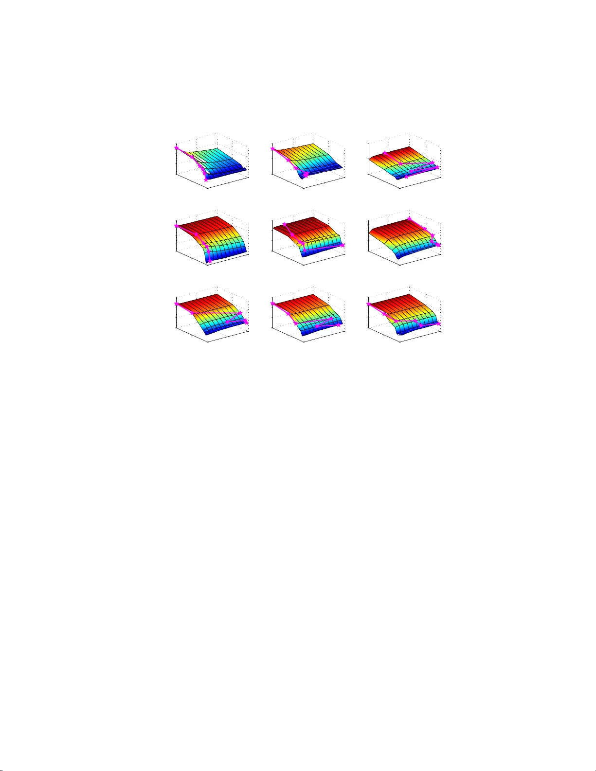
Sparsit y-accuracy trade-off in MKL Ry ota T omiok a & T aiji Suzuki ∗ { tomioka, t-suzuki } @mist .i.u-tokyo.ac.jp Abstract W e empirically inv estigate th e b est trade-off betw een sparse and un iformly- w eighted multiple kernel learning (MKL) using th e elastic-net regular- ization on real and sim u lated datasets. W e find that the b est t rade-off parameter d ep en ds n ot only on the sparsity of the true kernel-wei ght sp ec- trum but also on the linear dep endence among kernels and the number of samples. 1 In tro duction Sparse multiple k ernel learning (MKL; see [9, 12, 2]) is often outp e rformed by the s imple uniformly-weight ed MK L in terms of accuracy [3, 8]. Ho wev er the sparsity o ffered by the spar se MKL is helpful in understanding whic h feature is useful a nd can also sav e a lo t o f c o mputation in pr actice. In this pap er we inv estiga te this trade-off b etw een the sparsity and a ccuracy using an elastic-ne t t yp e regular ization term which is a smo oth interpola tion betw een the sparse ( ℓ 1 - ) MKL a nd the unifor mly-weigh ted MKL. In a ddition, w e ex tend the re c en tly prop osed SpicyMKL alg o rithm [15] for efficient optimization in the prop osed elastic-net regular iz ed MKL framework. Based on real and simulated MKL problems with more than 100 0 k e rnels, w e show that: 1. Spar se MKL indeed suffers from po or accuracy when the n umber of sam- ples is small. 2. As the num b e r of samples grows larger , the difference in the acc ur acy betw een spar se MKL and uniformly-weigh ted MKL becomes s maller. 3. Often the best accura cy is obtained in b etw een the sparse and uniformly- weigh ted MKL . This can b e explained by the dep endence among candidate kernels ha ving neigh b oring kernel parameter v alues. ∗ Both authors contributed equalit y to this work. 1 2 Metho d Let us assume that we ar e provided with M r epro ducing kernel Hilb ert spaces (RKHSs) equipp ed with kernel functions k m : X × X → R ( m = 1 , . . . , M ) and the task is to learn a classifier from N training examples { ( x i , y i ) } N i =1 , where x i ∈ X and y i ∈ {− 1 , +1 } ( i = 1 , . . . , N ). W e formulate this pr oblem into the following minimization problem: minimize f m ∈H m ( m =1 ,...,M ) , b ∈ R N X i =1 ℓ  m X m =1 f m ( x i ) + b, y i  + C M X m =1  (1 − λ ) k f m k H m + λ 2 k f m k 2 H m  , (1) where in the first term, f m is a member of the m - th RKHS H m , b is a bias term, and ℓ is a loss function; in this pap er w e use the log istic loss function. The second term is a r egulariza tion term a nd is a mixture of ℓ 1 - and ℓ 2 - re g ularization terms. The constant C ( > 0) determines the ov er all trade-o ff b etw een the loss term and the regularizatio n terms. Here the first regular ization term is the linear sum of RKHS norms, which is kno wn to make only few f m ’s non-zer o (i.e., sparse, see [16, 18, 1]); the second reg ularization ter m is the squared sum of RKHS no rms. The tw o regular ization terms ar e balanced by the cons tant λ (0 ≤ λ ≤ 1); λ = 0 corres p onds to sparse ( ℓ 1 -) MKL and λ = 1 corres po nds to unif ormly-weighted MKL. Due to the representer theorem (see [13]), the solutio n of the ab ov e minimiza- tion problem (1) takes the form f m ( x ) = P N i =1 k m ( x, x i ) α i,m ( m = 1 , . . . , M ); therefore we can equiv a lently solve the following finite-dimensional minimization problem: minimize α m ∈ R N ( m =1 ,...,M ) , b ∈ R L  M X m =1 K m α m + b 1  + C M X m =1  (1 − λ ) k α m k K m + λ 2 k α m k 2 K m  , (2) where K m ∈ R N × N is the m -th Gram matrix, α m = ( α 1 ,m , . . . , α N ,m ) ⊤ is the weigh t vector for the m -th kernel, and 1 ∈ R N is a vector o f all one; in addition, L ( z ) = P n i =1 ℓ ( z i , y i ) . Mo reov er, we define k α m k K m = p α m ⊤ K m α m . The minimization problem (1) is connected to the co mmonly use d “ le arning the ke rnel-weights ” form ula tion of MKL in the following wa y . Fir st let us define g ( x ) = (1 − λ ) √ x + λ 2 x for x ≥ 0 and g ( x ) = −∞ for x < 0. Since g is a concav e function, it ca n b e linearly upper-b ounded as g ( x ) ≤ xy − g ∗ ( y ), where g ∗ ( y ) is the c oncav e conjugate o f g ( x ). Th us s ubstituting x = k α m k 2 K m and y = 1 2 β m for m = 1 , . . . , M in Eq. (2), we ha ve: minimize α m ,b,β m L  M X m =1 K m α m + b 1  + C M X m =1  k α m k 2 K m 2 β m − g ∗  1 2 β m  , 2 where g ∗  1 2 β m  = − 1 2 (1 − λ ) 2 β m 1 − λβ m . Minimizing the a bove expressio n wr t α m while ke eping the loss t erm unchange d (i.e., P M m =1 K m α m = z for so me z ), we have α m = β m α ∗ and finally we can rewrite Eq. (2) as follows: minimize α ∗ ∈ R n ,b ∈ R , β ∈ R M L  K ( β ) α ∗ + b 1  + C 2  α ∗ ⊤ K ( β ) α ∗ + M X m =1 ˜ g ( β m )  , where K ( β ) = P M m =1 β m K m and ˜ g ( β m ) = − 2 g ∗ (1 / (2 β m )). Therefor e Eq. (2) is equiv alent to learning the decision function with a co m bined kernel K ( β ) with the Tikho nov regular ization on th e kernel weigh ts β m . Note that ˜ g ( β ) = β ( ℓ 1 -MKL) if λ = 0 and ˜ g ( β ) appro a ches the indicato r function of the closed int erv al [0 , 1 ] in the limit λ → 1 (uniformly-weighted MK L). In this pap er we call β = ( β m ) M m =1 a kernel-weight sp e ctr um . The regulariza tion in Eq. (1) is known as the elastic-ne t reg ularization [19]. In the co n text of MK L , Shaw e-T a ylor [14] prop ose d a similar appro a ch that uses the square of the linear sum of no rms in Eq. (2). Both Shaw e-T a ylor’s and our approach use mixed ( ℓ 1 - and ℓ 2 -) regularization o n the weight ve ctor (or its non-para metr ic version) in the hop e of curing the over-sparseness of ℓ 1 -MKL. There are alter native appro aches that a pply non- ℓ 1 -regular ization on the kernel weights β m . Longworth a nd Gales [11] used a combination of ℓ 1 -norm constraint and ℓ 2 -norm p enaliza tion on the kernel weigh ts. Klo ft et al. [8] pro - po sed to regularize the ℓ p -norm of the kernel weigh ts (see als o [4]). Our ap- proach (and [1 1]) differ fro m [8] in that we can o bta in different levels of sp arsity for all λ < 1 (see b ottom row o f Fig. 1), whereas for all p > 1 the resulting kernel-w eight sp ectrum is dense in [8]. Note also tha t uniformly-weigh ted MKL ( ϕ = ∞ in [11] and p = ∞ in [8]) corr esp onds to λ = 1 in o ur approa ch, which may b e a p os sible adv antage o f our approach. 3 Results 3.1 Real data W e computed 1 ,760 kernel functions on 10 binary imag e clas sification prob- lems (b etw een every combinations of “ anchor”, “ant”, “cannon” , “chair”, and “cup”) from Caltech 101 dataset [5]. The kernel functions were constructed as combinations o f the following four factors in the prep oss essing pipeline: • F our t yp es of SIFT features, namely hsv s ift (ada ptiv e s c a le), sift (adaptive scale), s ift (sca le fixed to 4px), sift (sca le fixed to 8px). W e used the implemen tation by v an de Sande et al. . [17]. The lo cal features were sampled uniformly (grid) from each input image. W e ra ndomly choo sed 3 200 lo c a l features a nd assigned visual words to every lo cal featur es using these 200 p oints as cluster cen ters. • Lo ca l histogra ms obtained by partitioning the imag e into rectangula r cells of the same size in a hier archical manner; i.e., level-0 pa r titioning ha s 1 cell (whole image) level-1 partitioning ha s 4 cells and level-2 partitioning has 16 cells . F rom each cell we computed a k ernel function by measuring the similarity of the tw o lo cal feature histo g rams computed in the sa me cell from tw o ima ges. In addition, the spatial-pyramid kernel [7, 1 0], which combines these k ernels by exp onentially decaying weigh ts, was computed. In total, we used 22 kernels (=o ne level-0 k ernel + four level-1 k e rnels + 16 lev el-2 kernels + one spatial-pyramid kernel). See also [6] for a similar approach. • Two kernel functions (similarit y measures). W e used the Gaus s ian kernel: k ( q ( x ) , q ( x ′ )) = exp  − n X j =1 ( q j ( x ) − q j ( x ′ )) 2 2 γ 2  , for 10 band-width parameter s ( γ ’s) line a rly spac e d betw een 0 . 1 and 5 and the χ 2 -kernel: k ( q ( x ) , q ( x ′ )) = exp  − γ 2 n X j =1 ( q j ( x ) − q j ( x ′ )) 2 ( q j ( x ) + q j ( x ′ ))  for 10 band-width parameters ( γ ’s) linearly spa ced b etw een 0 . 1 a nd 10 , where q ( x ) , q ( x ′ ) ∈ N n + are the histog rams computed in some reg ion of tw o images x and x ′ . The combination of 4 sift features, 22 spacia l regions, 2 kernel functions, a nd 10 parameters resulted in 1,760 kernel functions in total. Figure 1 sho w s the a verage classifica tion a ccuracy a nd the num ber of active kernels obtained at different v alues of the trade-off par ameter λ . W e ca n see that spar se MKL ( λ = 0) can b e significantly o utper formed by simple uniformly- weigh t MKL ( λ = 1) when the num b er of s a mples ( N ) is small. As the n umber of samples g rows the difference b et ween the t wo case s decr eases. Moreover, the bes t accuracy is obtained at more and more spar s e solutions as the num b er o f samples grows la r ger. 3.2 Sim ulated data In order to explain the results from the image-clas sification datas et in a simple setting, we genera ted three toy pro blems. In the first problem we placed one Gaussian kernel ov er each input v ar iable that w as independently sampled from the standa rd normal distribution. The num b er of input v aria bles w as 1 00. W e call this setting F e atur e sele ction . In the second problem w e increased the 4 0 0.5 1 0.7 0.8 0.9 lambda N=5 ACCURACY 0 0.5 1 0 500 1000 1500 2000 lambda # OF ACTIVE KERNELS 0 0.5 1 0.7 0.8 0.9 lambda N=15 ACCURACY 0 0.5 1 0 500 1000 1500 2000 lambda # OF ACTIVE KERNELS 0 0.5 1 0.7 0.8 0.9 lambda N=20 ACCURACY 0 0.5 1 0 500 1000 1500 2000 lambda # OF ACTIVE KERNELS 0 0.5 1 0.7 0.8 0.9 lambda N=30 ACCURACY 0 0.5 1 0 500 1000 1500 2000 lambda # OF ACTIVE KERNELS C=0.0001 C=0.001 C=0.01 C=0.1 C=0.5 Figure 1: Image classification results from Ca ltec h 1 01 da taset. The trade- off parameters λ that achieve the highest test accur acy are marked by stars. v ariety of k ernels by in tro ducing 12 kernels with different band-widths on each input v ariable. The num b er o f input v ar iables was 1 0. W e ca ll this s e tting F e atur e & Par ameter sele ction . In the thir d pro ble m, we used the same 1 2 kernel functions with different band-widths but jointly ov er the sa me set of 10 input v ariables. W e call this setting Par ameter sele ction . The tr ue kernel- weigh t sp ectrum ( β m ) M m =1 was changed from spar se (only tw o non- zero β m ’s), medium-dense (exp onentially decaying sp ectrum) to dense (unifor m sp ectrum). Figure 2 shows the test classificatio n accura cy obtained from training the prop osed elastic-net MKL mo del to nine toy-problems with differ e n t goa ls and different true kernel-weigh t sp ectra. W e choose the b est regularization constant C for each plot. First we can observe that w he n the goal is to choo se a subset of kernels from indep endent data -sources (top r ow), the b est trade-o ff para meter λ is mo stly deter mined by the true kernel-weigh t s pectr um; i.e., sma ll λ for spars e and large λ for dense spectrum. Rema rk ably the s parse MKL ( λ = 0) pe rforms well even when the num ber o f samples is smaller tha n that o f kernels if the true kernel-w eight sp ectrum is spars e . On the other hand, if we also consider the selectio n of kernel parameter thro ug h MKL (middle ro w), the b est trade-off parameter λ is often obtained in b etw een zero a nd one and seems to dep end less on the true k ernel-weight sp ectrum. This finding seems to b e consistent with the observ ation in [19] that the ela stic-net (0 < λ < 1) perfor ms well when the input v aria bles a re linearly dependent b ecause kernels that only differ in the band-width can hav e significant dependency to each other. F urthermo re, if we consider the sele c tio n of kernel para meter only (b ottom row), the accur acy bec omes almost flat for all λ r egardless of the true kernel-weigh t sp ectrum. The 5 0 0.5 1 0 50 100 0.4 0.6 0.8 1 lambda Sparse N Feature Selection ACCURACY 0 0.5 1 0 50 100 0.4 0.6 0.8 lambda Medium−Dense N ACCURACY 0 0.5 1 0 50 100 0.4 0.6 0.8 lambda Dense N ACCURACY 0 0.5 1 0 50 100 0.7 0.8 0.9 1 lambda N Feature & Parameter Selection ACCURACY 0 0.5 1 0 50 100 0.4 0.6 0.8 1 lambda N ACCURACY 0 0.5 1 0 50 100 0.4 0.6 0.8 1 lambda N ACCURACY 0 0.5 1 0 50 100 0.4 0.6 0.8 1 lambda N Parameter Selection ACCURACY 0 0.5 1 0 50 100 0.4 0.6 0.8 1 lambda N ACCURACY 0 0.5 1 0 50 100 0.4 0.6 0.8 1 lambda N ACCURACY Figure 2: Classification accuracy obtained from the simulated datasets. The magenta colo red curves with stars denote the v alue of tr ade-off parameter s λ that yield the highest test a ccuracy . behaviour in the Ca ltech dataset seems to b e most similar to the second column of the second row (feature & parameter selection under medium sparsity). 4 Summary In this pap er, we have e mpirically inv estigated the trade-off b etw een spa rse and uniformly-w eighted MKL using the ela stic-net t yp e reg ula rization ter m for MKL. The s parsity of the s olution is modula ted by changing the trade- off pa- rameter λ . W e consis tently found that, (a) often the unifor mly-weigh ted MKL ( λ = 1) outp erforms sparse MK L ( λ = 0 ); (b) the difference b etw een the tw o cases decrea s es as the nu mber of samples increases; (c) when the input kernels are indep endent, the sparse MKL seems to b e favorable if the true kernel-w eight sp ectrum is not too dense; (d) when the input kernels are linearly dep endent (e.g., kernels with neighbor ing pa r ameter v alue s are included), int ermediate λ v alue seems to be fav o rable. W e ha ve a lso o bserved tha t as the num b er o f s am- ples incr e ases the spars e r so lution (small λ ) is pr eferred. It was als o o bs erved (results not shown) that spar ser solutio n is preferred when the no ise in the training lab els is small. 6 References [1] F. Bach. Co nsistency o f the group la sso and m ultiple kernel lea rning. JMLR , 9:11 79–12 25, 2008 . [2] F. Bach, G. Lanckriet, a nd M. Jordan. Multiple kernel lear ning , conic duality , and the SMO algo rithm. In the 21st International Confer enc e on Machine L e arning , pages 41–48 , 2004. [3] C. Co rtes. Can learning kernels help p er formance? Invited talk at Interna- tional Co nference o n Machine Learning (ICML 2 009). Montr´ eal, Canada , 2009. [4] C. Cortes , M. Mohr i, and A. Ros ta mizadeh. L2 r egulariza tion for learning kernels. In Pr o c. UAI 2009 , J une 2009 . [5] L. F ei-F ei, R. F erg us, and P . Perona. Learning genera tive visua l mo dels from few tra ining examples: an incr ement al bay esian approach tested on 101 o b ject catego ries. In IEEE. CVPR 20 04 Workshop on Gener ative- Mo del Base d Vision , 2004 . [6] P . Gehler and S. Nowozin. Let the kernel figure it out; principled lea rning of pre-pro cessing f or kernel classifiers. In IEEE CVPR 2009 , 2 009. [7] K. Grauman a nd T. Darrell. The pyramid match kernel: E fficient lear ning with sets of features. JMLR , 8:72 5–760 , 2007 . [8] M. Kloft, U. B refeld, S. So nnenb urg, P . Lasko v, K.-R. M ¨ uller, and A. Z ien. Efficient and a ccurate lp-norm m ultiple kernel lear ning. In A dvanc es i n NIPS 22 . 2010 . [9] G. R. La nckriet, N. Cristianini, P . Bar tlett, L. E. Ghaoui, and M. I. Jordan. Learning the Ker nel Matrix with Semidefinite Progra mming . J. Machine L e arning Rese ar ch , 5:27–72 , 20 04. [10] S. Lazebnik, C. Sc hmid, and J. Ponce. Beyond ba gs of features: Spatial pyramid matc hing for recog nizing na tural scene categories. In Pr o c. IEEE CVPR , volume 2, pages 2169–2 178, 200 6. [11] C. Longworth a nd M. Gales. Combining deriv ative and parametric ker- nels for sp eaker verification. IEEE T r ansactions on Audio , Sp e e ch, and L anguage Pr o c essing , 1 7(4):748– 757, 200 9. [12] C. A. Micchelli and M. Pontil. Learning the kernel function via regular iza- tion. J . Mach. L e arn. R es. , 6:1099– 1125, 20 05. [13] B. Sc h¨ olkopf and A. Smola. L e arning with Kernels: Supp ort V e ctor Ma- chines, R e gularization, Optimization and Beyond . MIT Pre ss, Cam bridge, MA, 2002. 7 [14] J. Shawe-T aylor. Kernel lear ning for no velt y detection. In NIPS 08 W or k- shop: Kernel Learning – Automatic Selection of O ptimal Kernels, 2008 . [15] T. Suzuki and R. T omiok a . SpicyMKL. T echnical Rep o rt arXiv:0 909.50 26 , 2009. [16] R. Tibshirani. Regressio n s hrink age and selection via the lasso. J. R oy. Stat. So c. B , 58 (1 ):267–2 88, 19 9 6. [17] K. E . A. v an de Sande, T. Gev ers, and C. G. M. Sno e k . Ev aluating colo r descriptors for ob ject and scene r e c ognition. IEE E T r ansactions on Pattern Analy sis and Machine Intel ligenc e , (in pr ess), 2010. [18] M. Y uan and Y. Lin. Mo del selection and estimation in r egressio n with group ed v aria bles. J. R oy. St at. So c. B , 68 (1):49–6 7 , 20 06. [19] H. Zou and T. Hastie. Regularization and v ariable selection via the elastic net. Journ al of the R oyal Statistic al So ciety S eries B(Statistic al Metho dol- o gy) , 6 7(2):301– 320, 200 5. 8