Static Hopfions in the extended Skyrme-Faddeev model

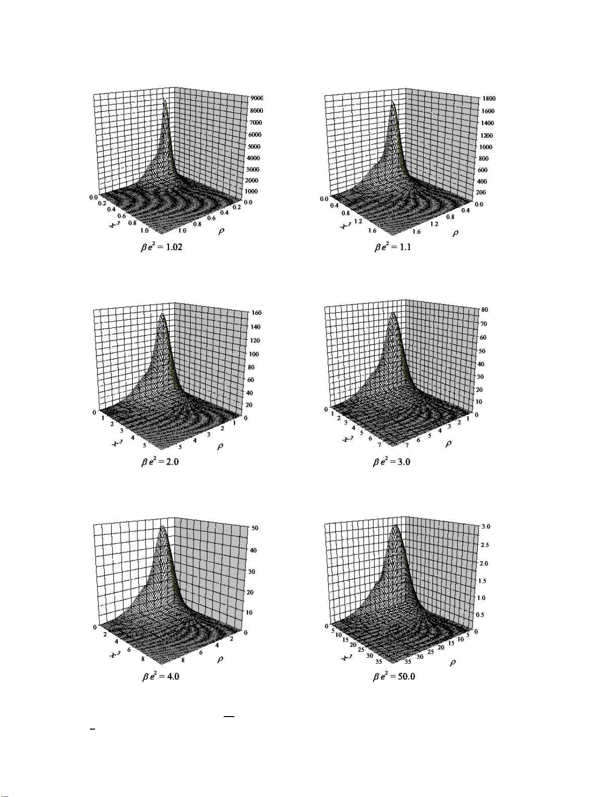
Static Hopfions in the extended Skyrme-F addeev mo del L. A. F erreira a , ∗ Nobuyuki Saw ado a,b , † and Kouichi T o da a,c ‡ a Instituto de F ´ ısic a de S˜ ao Carlos; IFSC/USP, Universidade de S˜ ao Paulo - USP, Caixa Postal 369, CEP 13560-970, S˜ ao Carlos-SP, Br azil b Dep artment of Phys ics, T okyo University of Scienc e, No da, Chib a 278-8510, Jap an c Dep artment of Mathemat ic al Physics, T oyama Pr efe ctur al University, Kur okawa 5180, Imizu, T oyama, 939-0398, Jap an (Dated: June 2, 2018) W e construct static soli ton solutions with non-zero Hopf topological c harges to a theory w hich is an extension of the Skyrme-F add eev mo del by the addition of a further quartic t erm in deriv ativ es. W e use an axially symmetric ansatz based on toroidal co ordinates, and solve the resulting t w o coupled non-linear partial differen tial eq uations in tw o vari ables by a successiv e o ver-rela xation (SOR) metho d . W e construct numerical solutions with Hopf charge up to four, and calculate their analytical b ehavio r in some limiting cases. The solutions present an interes ting b eha vior under the changes of a sp ec ial combinatio n of the coupling constants of the q uartic terms. Their energies and sizes tend to zero as th at combination approac hes a particular sp ecial v alue. W e calculate the equiv alen t of th e V akulenko and Kapitanskii energy bound for the t heory and find th at it va nishes at that same sp ecial v alue of th e coupling constants. In addition, th e mo del presents an integrable sector with an infin ite number of local conserved currents which app a rently are not related to symmetries of t he action. In t he in tersection of those tw o special sectors the theory p ossesse s exact vortex solutions (static and time d ependent) whic h were constru cted in a previous pap er by one of the authors. It is b elie ved that such mod el describes some aspects of the lo w energy limit of the pure SU(2) Y ang-Mills theory , and our results ma y be important i n iden tifying imp ortan t stru ctures in th at strong coupling regime. I. INTRO DUCTION W e construct static soliton solutions, ca rrying no n-trivial H opf top ological c harges , for a field theory that has found int eresting applicatio ns in many areas of Ph ysics. It is a (3 + 1)-dimensional Lorentz inv ar ian t field theory for a triplet of scalar fields ~ n , liv ing on the tw o-sphere S 2 , ~ n 2 = 1, a nd defined by the Lagrangia n dens ity L = M 2 ∂ µ ~ n · ∂ µ ~ n − 1 e 2 ( ∂ µ ~ n ∧ ∂ ν ~ n ) 2 + β 2 ( ∂ µ ~ n · ∂ µ ~ n ) 2 (1) where the coupling co nstan ts e 2 and β are dimensionless, a nd M has dimension o f mas s. The firs t tw o terms corres p ond to the so-called Sk yrme-F addeev (SF) mo del [1], w hich was prop osed long ago following Skyrme’s idea [2], as the generaliza tion to 3 + 1 dimens ions of the C P 1 mo del in 2 + 1 dimensions [3]. The in terest in the SF mo del has grown co nsiderably in re c en t years since the first numerical kno tted soliton solutions were c o nstructed [4, 5, 6, 7, 8], as well as vortex type solutions [9, 10]. It has also found applicatio ns in Bo s e-Einstein c ondensates [11], sup e rconductors [12, 13] and in the W einberg-Sa lam mo del [14]. In addition, it has be en conjectured by F addeev and Niemi [15] that the SF mo del descr ibes the low energ y (stro ng coupling ) r egime of the pure S U (2) Y ang-Mills theory . That was based on the so -called C ho -F addeev- Niemi- Sha bano v decomp osition [15, 16, 1 7 , 18] of the S U (2) Y ang-Mills field ~ A µ , where its six physical degrees of freedom a re enco ded into a triplet o f scalars ~ n ( ~ n 2 = 1), a mas sless U (1 ) gauge field, and tw o real scalar fields. The motiv ation for such de c o mposition o riginates fro m the fact that the triplet ~ n can be used as an order par a meter for a condensate of W u-Y ang monop oles, which cla ssical solution can then b e written as ~ A 0 = 0, ~ A i = ∂ i ~ n ∧ ~ n , i = 1 , 2 , 3, with ~ n co rrespo nding to the hedgehog configuration ~ n = ~ x/r . The conjecture of F addee v a nd Niemi requires non-p erturbative calculations to b e pr o v ed or disprov ed and s o the discussions in the litera ture hav e been quite controv ersial. Lattice field theory simulations hav e discourage d its v alidit y [19], and recently F addeev himself has propo sed some mo difications for it [20]. Gies [21] has calculated the one-lo op Wilsonian effective action for the S U (2) Y a ng-Mills theory , using the Cho- F addeev- N iemi-Shabanov decompos ition, ∗ Electronic address: laf@ifsc.usp.br † Electronic address: sa wado@ph.noda.tus.ac.jp ‡ Electronic address: k ouichi@yuk aw a.ky oto-u.ac.jp 2 and found a greemen ts with the conjecture provided the SF mo del is mo dified by a dditio na l quartic terms in deriv a tiv es of the ~ n field. In fa c t, Gies obtained an effective action which up to first der iv atives of ~ n is of the form (1). Similar results were obtained in [22] for the c onnection b e t ween the low ener g y Y ang-Mills dyna mics and mo difications of Skyrme-F addeev mo del using the Gauss ian approximation of the v acuum wa v e functional. In this sense the extended version of the Sk y rme-F addeev mo del given by the theory (1 ) deserves s ome attention. Like the SF mo del it pr esen ts the internal O (3) symmetry and admit so lutions with top ology given by the Hopf ma p S 3 → S 2 . The main difference is the fact that (1) contains qua rtic terms in time deriv ativ es a nd s o its canonical Hamiltonian is not po sitiv e definite when hard mo des of the ~ n field a re allow ed. Indeed, that is a feature of many low energy effectiv e theo r ies. The theor y (1) has many in teresting aspe cts which deser v es a tten tio n a s we now expla in. It has tw o sector s wher e the s tatic energy density is p ositive definite and one o f them intersects with an integrable sub-sector o f (1) with a n infinite num be r of conserv a tion laws. In a Mink owiski space-time the static Hamiltonian asso ciated to (1) is H static = M 2 ∂ i ~ n · ∂ i ~ n + 1 e 2 ( ∂ i ~ n ∧ ∂ j ~ n ) 2 − β 2 ( ∂ i ~ n · ∂ i ~ n ) 2 (2) with i, j = 1 , 2 , 3. Therefore , it is p ositive definite for M 2 > 0, e 2 > 0 a nd β < 0 . That is the secto r explore d in [23], and wher e static soliton so lutions with non-trivial Hopf top o logical charges were constr uc ted. One can now stereogr aphic pro ject S 2 on a pla ne and work with a complex scalar field u related to the triplet ~ n by ~ n = 1 1+ | u | 2  u + u ∗ , − i ( u − u ∗ ) , | u | 2 − 1  (3) It then follows that ~ n · ( ∂ µ ~ n ∧ ∂ ν ~ n ) = 2 i ( ∂ ν u∂ µ u ∗ − ∂ µ u∂ ν u ∗ ) (1+ | u | 2 ) 2 ( ∂ µ ~ n · ∂ µ ~ n ) = 4 ∂ µ u ∂ µ u ∗ (1+ | u | 2 ) 2 (4) Therefore, in terms of the field u the Lagr angian (1) reads L = 4 M 2 ∂ µ u ∂ µ u ∗ (1+ | u | 2 ) 2 + 8 e 2 " ( ∂ µ u ) 2 ( ∂ ν u ∗ ) 2 (1+ | u | 2 ) 4 +  β e 2 − 1  ( ∂ µ u ∂ µ u ∗ ) 2 (1+ | u | 2 ) 4 # (5) The same static Hamiltonian (2) is now written as H static = 4 M 2 ∂ i u ∂ i u ∗ (1+ | u | 2 ) 2 − 8 e 2 " ( ∂ i u ) 2 ( ∂ j u ∗ ) 2 (1+ | u | 2 ) 4 +  β e 2 − 1  ( ∂ i u ∂ i u ∗ ) 2 (1+ | u | 2 ) 4 # (6) Therefore, it is p o sitiv e definite for M 2 > 0 ; e 2 < 0 ; β < 0 ; β e 2 ≥ 1 (7) It is that sector that we sha ll co nsider in this pa per. W e show that it p ossesses static soliton solutio ns with non- trivial Hopf to pologica l c harge. If one compar es (1) with the effectiv e Lag rangian given by eq. (14) or (21) o f [21] one observes that, in o rder for them to agree, e 2 and β should indeed hav e the same sig n. In the physical limit where the infrared cutoff go es to zero it follows that they both b e c ome p ositive, contrary to our assumption. How ev er, the per turbativ e calculations in [21] ar e not v alid in that limit, and s o no t muc h can b e said even ab out their rela tiv e signs. An interesting study o f such sector was p e rformed in [2 4] with an a ddit ional term in the action containing second deriv a tiv es of the ~ n field a nd corr e s ponding to the extr a term obtained in [21] when the hard mo des of ~ n ar e also in tegrated out. Another interesting asp ect of the theory (1) has to do with its integrability prop erties. The Euler -Lagrange equations following from (5), or equiv alently (1), reads  1+ | u | 2  ∂ µ K µ − 2 u ∗ K µ ∂ µ u = 0 (8) together with its complex conjugate, a nd wher e K µ ≡ M 2 ∂ µ u + 4 e 2  β e 2 − 1  ( ∂ ν u ∂ ν u ∗ ) ∂ µ u + ( ∂ ν u∂ ν u ) ∂ µ u ∗  (1+ | u | 2 ) 2 (9) 3 The theory (1) has three co nserv ed currents asso ciated the O (3) internal symmetry . How ev er, using the tec hniques of [25, 26] one ca n show that the sub-s e ctor defined by the constraint ∂ µ u ∂ µ u = 0 (10) po ssesses an infinite num ber of conserved currents g iv en by J µ ≡ δ G δ u K c µ − δ G δ u ∗ K c µ ∗ (11) where G is any function of u and u ∗ , but not of their deriv atives, and K c µ is obtained from (9) b y imp osing (10), i.e. K c µ ≡ M 2 ∂ µ u + 4 e 2  β e 2 − 1  ( ∂ ν u ∂ ν u ∗ ) ∂ µ u (1+ | u | 2 ) 2 (12) The fact that currents (11) are conserved follows from the ident ity I m ( K µ ∂ µ u ∗ ) = 0, the condition K c µ ∂ µ u = 0 following from (10), and the equations of motion, which no w rea d ∂ µ K c µ = 0. If in addition of (10) one restricts to the sector where the coupling constant s sa tisfy β e 2 = 1 (13) then the e quations of motion simplify to ∂ 2 u = 0, and the theory b ecomes scaling inv ariant. That co nstit utes a n int egrable sub-se c to r of the theory (1). Exa ct vortex solutions were constructed in [27], using quite s imple and direc t metho ds. One can hav e multi-v ortex solutions all lying in the sa me direction, and the v ortices can b e either static or hav e wav es tr a v eling along them with the sp eed o f light. Apparently the integrable sub- sector defined by conditions (10) a nd (13) do not admit soliton solutions with non- trivial Hopf top ological charges. In this pa p er we cons tr uct such solito ns for the theory (1) in the rang e of the co uplin g constants defined in (7) and witho ut imp osing the co ns train t (10). W e construct static solutions with a xial sy mm etry by solving numerically the equa tions of motion. Due to the axial symmetry w e ha ve to solve tw o coupled non- linea r partial differen tial equa tions in t w o dimensio ns. W e cho ose to use the tor oidal co ordinates defined as x 1 = r 0 p √ z cos ϕ x 2 = r 0 p √ z sin ϕ p = 1 − co s ξ √ 1 − z x 3 = r 0 p √ 1 − z sin ξ (14) where x i , i = 1 , 2 , 3, ar e the Car tesian co ordinates in I R 3 , and ( z , ξ , ϕ ) ar e the toroida l co ordinates. W e hav e 0 ≦ z ≦ 1, − π ≦ ξ ≦ π , 0 ≦ ϕ ≦ 2 π , and r 0 is a free parameter with dimension o f length. Notice that the usual toroidal c oordinates ha ve a co ordinate η > 0 which is related to our z by z = ta nh 2 η . W e constr uct solutions which ar e inv ariant under the diagona l U (1 ) subgroup of the direct pro duct o f the U (1) group of rotations on the x 1 x 2 plane and the U (1) group of in ternal phase transformations u → e i α u . W e then use the ansatz u = s 1 − g ( z , ξ ) g ( z , ξ ) e i Θ( z,ξ )+ i n ϕ (15) with n b eing an integer, and 0 ≤ g ≤ 1, − π ≤ Θ ≤ π . By r escaling the Cartesian co ordinates as x i → x i /r 0 , it is then clea r that the eq ua tions of motio n (8) will depe nd only up on t w o dimensio nless parameter s , namely β e 2 ≥ 1 a nd a 2 = − e 2 r 2 0 M 2 > 0 (16) since we are assuming (7). In a ddition, fr om (6) the static energy can b e written as E = Z d 3 x H static = 4 M | e | h E 2 + 2  E (1) 4 +  β e 2 − 1  E (2) 4 i (17) 4 in terms of the dimensionless qua n tities E 2 = M | e | Z d 3 x ∂ x i u ∂ x i u ∗ (1+ | u | 2 ) 2 E (1) 4 = 1 M | e | Z d 3 x | ( ∂ x i u ) 2 | 2 (1+ | u | 2 ) 4 (18) E (2) 4 = 1 M | e | Z d 3 x ( ∂ x i u ∂ x i u ∗ ) 2 (1+ | u | 2 ) 4 By replacing the a ns atz (15) in to the equa tions of mo tion (8) we get t wo non-linear partial differ en tial equations for the function g ( z , ξ ) a nd Θ ( z , ξ ), dep ending upon the dimensionless parameter s β e 2 and a . W e solve those equations numerically using a standard relaxatio n metho d [28], with appropria te bo undary conditions explained below. Derrick’s argument [2 9] implies that the co n tribution to the energ y from the quadra c t ic a nd quartic terms m ust equal, i.e. E 2 = 2  E (1) 4 +  β e 2 − 1  E (2) 4  (see (17)) . That fixes the size o f the solution a nd so the v alue of a . Therefore, in our nu merical pr ocedure we de ter mine a on each step of the relaxa t ion metho d using Derrick’s argument. Our main results are the following. W e find finite energy axially symmetric so lutio ns with Hopf charges up to four. The a x ial s ymmetry comes from the use of the ansatz (15). Therefore, o ur solutions are not necessarily the ones with the low est pos sible ener gy for a g iv en v alue of the Hopf charge. F or the Skyr me-F addeev mo del the solutions with Hopf c harge 1 and 2 do pr esen t a xial symmetry [4 , 5, 6, 7, 8]. W e b eliev e the same may happ en in the extended mo del (1). An interesting discovery we made is that a → 0 as β e 2 → 1 . That mea ns that the so lutions shrink in that limit, and disapp ear for β e 2 = 1. In addition, the energ y also v anishes in the limit β e 2 → 1. Since all three terms in the ener gy (1 7 ) ar e p ositiv e they each v anish in that limit, including E (2) 4 , despite the factor  β e 2 − 1  in front of it. Another interesting discovery is that E (1) 4 is very small compar ed to the other tw o terms. In fact, fo r a wide range of the par ameter β e 2 we hav e E (1) 4 E 2 + 2  E (1) 4 + ( β e 2 − 1) E (2) 4  ∼ 10 − 3 Notice that E (1) 4 is a go od meas ur e o f how close the solutions a re of satisfying the constra in t (10). Ther efore our solutions are very clos e of belong ing to the integrable sector p ossessing the infinite num ber of c onserv ed currents given by (11). It would b e very interesting to perfo r m calcula tio ns with a finer mesh to impr ove the precisio n of that ratio. O ne thing is c lear how ev er, the clo s er is β e 2 to unity the b etter the constra int is sa tisfied by the solutions. How ev er, the so lutions shr ink in that limit. The Hopfions then dis appear and seem to g iv e pla ce to the vortex solutio ns constructed in [27]. That po in t cer tainly deser v es further studies. It would b e very desir a ble to p e rform simulations to see how the v ortices of [27] b ehav e when the conditions (10) and (13) are relaxed, and that fact is now under inv estigation. The pap er is org anized a s follows: in section I I we calc ula te the Hopf top ological charges for the configur ations within the a ns atz (15), in section I II we calculate a b ound for the static energ y (17) using methods s imilar to those of references [32, 3 3 ] employ ed in case o f the Skyrme-F addeev mo del. The e q uations of motion in terms of the a nsatz functions g ( z , ξ ) and Θ ( z , ξ ) a re calculated in section IV, and in s ection V we analyze the pr operties of the solutions in thr ee limiting cases, at spa tial infinity , at the circle x 2 1 + x 2 2 = r 2 0 , with x 3 = 0, and a ls o at the x 3 -axis. The nu merical methods and solutions a re descr ibed in s e ction VI. II. THE HOPF TOPOLOGICAL CHAR GE The static solutions of the theor y (1) define maps from the three dimensiona l space I R 3 to the target space S 2 . In order to ha ve finite ener gy solutions we need the fields to go to a v acuum config uration at spatial infinit y , and so we need ~ n → co nstan t for r → ∞ , with r b eing the distance to the origin of the co ordinate system. The r efore, finite energ y solutio ns map all p oin ts at spatial infinit y to a fixed p oin t o f S 2 . Consequen tly , a s far as the topolo gical prop erties o f such maps are concer ned we can iden tify the po in ts at infinity a nd consider the space to be S 3 instead of I R 3 . Then the finite ener gy solutions define maps S 3 → S 2 , and those are classified in to homotopy classes labe le d by a n integer Q H called the Hopf index. Such index can b e calcula ted thro ugh an integral formula a s follows [3 0 , 31]. W e first consider the mapping of the three dimensional space I R 3 int o a 3-spher e S 3 Z , pa rametrized by t w o co mplex nu mbers Z k , k = 1 , 2 , s uc h that | Z 1 | 2 + | Z 2 | 2 = 1. Using the ansa tz (15) we choo se such ma p to b e given by I R 3 → S 3 Z : Z 1 = p 1 − g e i Θ Z 2 = √ g e − i n ϕ (19) 5 W e then map suc h 3- sphere into the target S 2 by S 3 Z → S 2 : u = Z 1 Z 2 (20) In fact, the mapping of the plane parametr ized by the complex field u into the S 2 , para metrized by the triplet o f scalar fields ~ n , is given by the the stereog raphic pro jection defined in (3). The Ho pf index of such map is given by [30] Q H = 1 4 π 2 Z d 3 x ~ A ·  ~ ∇ ∧ ~ A  (21) with ~ A = i 2 2 X k =1 h Z ∗ k ~ ∇ Z k − Z k ~ ∇ Z ∗ k i (22) and w her e the integral is ov er the c oordinates x i of the three dimensiona l s pace I R 3 . Even though ~ A canno t b e wr itt en lo cally in terms of u or ~ n , its curv ature ca n. Indeed, from (4), (20) and (2 2 ) w e hav e F ij ≡ ∂ i A j − ∂ j A i = 1 2 ~ n · ( ∂ i ~ n ∧ ∂ j ~ n ) = i ( ∂ j u∂ i u ∗ − ∂ i u∂ j u ∗ ) (1+ | u | 2 ) 2 (23) Therefore the Hopf index (21) can alternatively b e written as Q H = 1 8 π 2 Z d 3 x ε ij k A i F j k (24) Performing the calculation using the toroidal co ordinates (14) we find that ~ A = p r 0  − 2 p z (1 − z ) (1 − g ) ∂ z Θ ~ e z − (1 − g ) √ 1 − z ∂ ξ Θ ~ e ξ + n g √ z ~ e ϕ  (25) where ~ e z , ~ e ξ and ~ e ϕ are the unit vectors in the direction of the changes of the p osition vector ~ r under v ar iations of co ordinates, i.e. ~ e z = ∂ z ~ r / | ∂ z ~ r | , and so on. The metric and volume element in toroidal co ordinates (14) are ds 2 =  r 0 p  2  dz 2 4 z (1 − z ) + ( 1 − z ) dξ 2 + z dϕ 2  d 3 x = 1 2  r 0 p  3 dz dξ dϕ (26) Therefore the Hopf index (21) for the field configur ations in the ansatz (15) is given by Q H = n 2 π Z 1 0 dz Z π − π dξ [ ∂ z ( g ∂ ξ Θ) − ∂ ξ ( g ∂ z Θ)] (27) W e now imp ose the bo undary conditions g ( z = 0 , ξ ) = 0 g ( z = 1 , ξ ) = 1 for − π ≤ ξ ≤ π (28) and Θ ( z , ξ = − π ) = − m π Θ ( z , ξ = π ) = m π for 0 ≤ z ≤ 1 (29) with m b eing an integer. It then follows that ∂ z Θ | ξ = − π = ∂ z Θ | ξ = π = 0, a nd s o from (27) Q H = m n (30) 6 II I. THE ENERGY BOUND The static energ y of the theory (1) in the regime (7) satisfy an ener gy b ound very similar to that one found b y V akulenk o and Kapitansk ii [3 2 ] for the Skyrme- F addeev mo del. The a rgumen ts ar e quite simple, a nd we start by the definition of F ij in (23) which implies that F 2 ij = 2 ( ∂ i u ∂ i u ∗ ) 2 (1+ | u | 2 ) 4 − 2 | ( ∂ i u ) 2 | 2 (1+ | u | 2 ) 4 (31) and so ∂ i u ∂ i u ∗ (1+ | u | 2 ) 2 ≥ s F 2 ij 2 (32) W e now rewr ite the static energy de ns it y (6) as H static = 4 M 2 ∂ i u ∂ i u ∗ (1+ | u | 2 ) 2 − 4 e 2  β e 2 − 1  F 2 ij − 8 β | ( ∂ i u ) 2 | 2 (1+ | u | 2 ) 4 (33) Therefore, us ing (32) and working in the regime (7) one has H static ≥ 4 M 2 s F 2 ij 2 − 4 e 2  β e 2 − 1  F 2 ij (34) Notice that the bounds (32) and (34) are saturated b y tho se configur ations satisfying the constraint (10). Therefore we s ho uld ex pect the solutions to b e driven in the dir ection of satisfying that constr ain t, and that is what w e find in our n umerical simulations. The static energ y (1 7 ) should then satisfy (assuming the regime (7)) E ≥ 2 11 / 4 M | e | p β e 2 − 1  Z d 3 x q F 2 ij  1 / 2  Z d 3 x F 2 ij  1 / 2 + " 2 M 2 1 / 4  Z d 3 x q F 2 ij  1 / 2 − 2 | e | p β e 2 − 1  Z d 3 x F 2 ij  1 / 2 # 2 W e now use the Sob olev-type inequalit y [3 2 , 33]  Z d 3 x q F 2 ij   Z d 3 x F 2 ij  ≥ 1 C  1 8 π 2 Z d 3 x ε ij k A i F j k  3 / 2 (35) where C is a univ ersal consta n t. W e then get the energy b ound E ≥ 2 11 / 4 C 1 / 2 M | e | p β e 2 − 1 Q 3 / 4 H where w e hav e used (24). The v alue o f C found in [33, 3 4 ] is 1 C = 8 3 3 / 4 √ 2 π 4 How ev er, W ard in [33] conjectures that a better v alue is 1 C = 64 √ 2 π 4 (36) T aking W ard’s v alue (36) one then gets the b ound E ≥ 64 π 2 M | e | p β e 2 − 1 Q 3 / 4 H (37) Notice that one s hould ex pect a decrea s e in the ener gy of the hopfions as β e 2 approaches unity , and that is e xactly what w e find in our numerical calculatio ns. 7 IV. THE EQUA TIONS OF MOTION By replacing the a ns atz (15) in to the equa tions of mo tion (8) we get t wo partial non-linear differ en tial equations for the functions g ( z , ξ ) a nd Θ ( z , ξ ). They are given by g (1 − g ) h 4( z (1 − z )) 2 ( p∂ z R z − R z ∂ z p ) + z ( p∂ ξ R ξ − R ξ ∂ ξ p ) i − (1 − 2 g ) p h 3 2  4  z (1 − z )  2 R z ∂ z g + z R ξ ∂ ξ g  − g (1 − g )  4  z (1 − z )  2 S z ∂ z Θ + z S ξ ∂ ξ Θ + (1 − z ) S ϕ n i = 0 (38) and g (1 − g ) h 4( z (1 − z )) 2 ( p∂ z S z − S z ∂ z p ) + z ( p∂ ξ S ξ − S ξ ∂ ξ p ) i − (1 − 2 g ) p h 3 2  4  z (1 − z )  2 S z ∂ z g + z S ξ ∂ ξ g  + g (1 − g )  4  z (1 − z )  2 R z ∂ z Θ + z R ξ ∂ ξ Θ + (1 − z ) R ϕ n i = 0 (39) with p b eing defined in (14) and where R z := − 1 2  g (1 − g ) z (1 − z ) + α ( v a − v b ) + γ ( v a + v b )  ∂ z g − αg (1 − g ) v c ∂ z Θ R ξ := − 1 2  g (1 − g ) z (1 − z ) + α ( v a − v b ) + γ ( v a + v b )  ∂ ξ g − αg (1 − g ) v c ∂ ξ Θ R ϕ := − αg (1 − g ) v c n S z := g (1 − g )  g (1 − g ) z (1 − z ) − α ( v a − v b ) + γ ( v a + v b )  ∂ z Θ + 1 2 αv c ∂ z g S ξ := g (1 − g )  g (1 − g ) z (1 − z ) − α ( v a − v b ) + γ ( v a + v b )  ∂ ξ Θ + 1 2 αv c ∂ ξ g S ϕ := ng (1 − g )  g (1 − g ) z (1 − z ) − α ( v a − v b ) + γ ( v a + v b )  where α := 4 p 2 a 2 γ := 4 p 2 a 2 ( β e 2 − 1) (40) and v a := 1 4  4( z (1 − z )) 2 ( ∂ z g ) 2 + z ( ∂ ξ g ) 2  v b := ( g (1 − g )) 2  4( z (1 − z )) 2 ( ∂ z Θ) 2 + z ( ∂ ξ Θ) 2 + (1 − z ) n 2  v c := g (1 − g )  4( z (1 − z )) 2 ( ∂ z g )( ∂ z Θ) + z ( ∂ ξ g )( ∂ ξ Θ)  (41) Besides the b oundary conditions (28) and (2 9 ) lea ding to the Hopf index g iv en by (30), we imp ose as well the additional bo undary conditions ∂ ξ g ( z , ξ ) | ξ = − π = ∂ ξ g ( z , ξ ) | ξ = π = 0 , for 0 ≤ z ≤ 1 (42) ∂ z Θ( z , ξ ) | z =0 = ∂ z Θ( z , ξ ) | z =1 = 0 , for − π ≤ ξ ≤ π (43) Notice that the equations of motion (38) a nd (39) are inv aria n t under the transformations ξ ↔ − ξ g ( z , ξ ) ↔ g ( z , − ξ ) Θ ( z , ξ ) ↔ − Θ ( z , − ξ ) (44) Therefore, we c ho ose the b oundary conditions ∂ ξ g ( z , ξ ) | ξ =0 = 0 , Θ( z , ξ = 0) = 0 (45) and perfo r m our numerical calcula tions on the half-plane defined b y 0 ≤ z ≤ 1 and 0 ≤ ξ ≤ π . The functions on the other half-plane, namely 0 ≤ z ≤ 1 and − π ≤ ξ ≤ 0 , a re obtained from the symmetry (4 4 ). 8 V. THE BEHA VIOR OF T HE SOLUTIONS IN LIMITING CASES The solutions within the ansatz (15) hav e axial symmetry aro und the x 3 -axis. In addition, from (3) and (15) one observes that the condition n 3 = constant implies g = constant . The numerical solutions sa tis fying the b oundary conditions (2 8 ), (29), (42), (4 3) and (4 5), that we find are such that for a giv en v alue of ξ , g is a monoto nically increasing function of z . In addition, for a g iven v alue of z , g do es not v ar y much under v ariations of ξ . It then turns out that the s urfaces in I R 3 corres p onding to constant n 3 hav e a toroida l s hape. They are in fac t deformations of the toroidal surfac e s obtained by fixing z and v arying ξ and ϕ (see (14)). It is then impor tan t to analyze the b ehavior of the so lutions in three regions, namely the spatial infinity and close to the x 3 -axis where due to the b oundary co ndit ion (28) we have n 3 = 1, and c lo se to the cir cle on the x 1 x 2 -plane of radius r 0 and centered at the origin, where n 3 = − 1. W e now p erform such analy sis. A. The b eha vior at spatial infinity ¿F r om (14) one o bserv es that r 2 ≡ x 2 1 + x 2 2 + x 2 3 = r 2 0  1 + √ 1 − z cos ξ   1 − √ 1 − z cos ξ  Therefore, in the toroidal co ordinates (14) the limit r → ∞ corre sponds to the double limit z → 0 and ξ → 0. W e choose to p erform such double limit through the para metr ization z ∼ ε 2 1 cos 2 σ ξ ∼ ε 1 sin σ with ε 1 → 0 0 ≤ σ ≤ π 2 (46) That corresp onds to p olar co ordinates o n the plane ( √ z , ξ ), and the deriv ativ es ar e related b y ∂ z = 1 2 ε 2 cos σ ( ε cos σ ∂ ε − sin σ ∂ σ ) ∂ ξ = sin σ ∂ ε + cos σ ε ∂ σ T aking into acco un t the b oundary co ndit ions (28), (43) and (45) we then assume the fields to b eha ve as g ∼ ε s 1 1 f ( σ ) Θ ∼ ε r 1 1 h ( σ ) (47) where s 1 and r 1 are co ns tan ts, and with the test functions satisfying f  π 2  = 0 f ′ (0) = 0 h (0) = 0 h ′  π 2  = 0 (48) where primes denote deriv atives w.r.t. σ . Replacing the expansions (47) in to the equations of mo tion (38) and (39), and k eeping only the leading terms, i.e. those with the smallest p ossible pow er o f ε 1 , we get the following equa tions for the test functions  f ′ f  ′ + 1 2  f ′ f  2 − tan σ f ′ f + 1 2 s 1 ( s 1 − 2) − 2 n 2 cos 2 σ = 0 (49) and h ′′ h +  f ′ f − tan σ  h ′ h + r 1 ( r 1 + s 1 − 1) = 0 (50) A s olution of (49) sa tis fying the boundar y conditions (48) is given by f ∼ (cos σ ) 2 | n | with s 1 = 2 ( | n | +1) (51) Replacing (51) into (50) and p erforming the change o f v ariables x = sin 2 σ 0 ≤ σ ≤ π 2 0 ≤ x ≤ 1 9 we g et that the equation (50) beco mes an h yperg eometric equation of the form x ( 1 − x ) ∂ 2 x h + 1 2 [1 − (2 | n | +3) x ] ∂ x h + 1 4 r 1 ( r 1 + 2 | n | +1) h = 0 (52) The boundar y conditions (48) imply that h | x =0 = 0 ∂ x h | x =1 = finite (53) There are tw o indep enden t s o lutions for equation (52), namely h 1 = F  | n | + r 1 + 1 2 , − r 1 2 , 1 2 , x  h 2 = x 1 / 2 F  | n | + r 1 2 + 1 , − r 1 2 + 1 2 , 3 2 , x  where F ( α, β , γ , x ) is the Gauss hypergeo metric s eries. O ne can chec k that such series do es not conv erge since in bo th cases w e ha ve α + β − γ = | n |≥ 1. W e then have to choose r 1 in order to trunca te the series. That leads us to the allo wed v alues for r 1 r 1 = 2 l + 1 l = 0 , 1 , 2 , . . . Since the first term o f F is 1, we se e that only h 2 satisfies the boundar y condition (53). Therefore, the a llo w ed solutions for Θ are Θ ∼ ε 2 l +1 1 sin σ F  | n | + l + 3 2 , − l , 3 2 , sin 2 σ  l = 0 , 1 , 2 , . . . In our n umerical ca lculations only solutions corresp onding to l = 0 appea r (so F = 1 ), and therefore the behavior o f our solutions at spatial infinit y , i.e. z , ξ ∼ 0, is giv en by g ∼ ε 2( | n | +1) 1 (cos σ ) 2 | n | ∼ z | n |  z + ξ 2  Θ ∼ ε 1 sin σ ∼ ξ (54) That implies that the u field at spatial infinity b ehav es a s u → 1 (2 r 0 ) | n | +1 r 2 | n | +1 ρ | n | e i n ϕ (55) with ρ 2 = x 2 1 + x 2 2 , and r 2 = x 2 1 + x 2 2 + x 2 3 . Therefore, we indeed hav e ~ n → (0 , 0 , 1), as r → ∞ . B. The b eha vior around the ci rcle x 2 1 + x 2 2 = r 2 0 , and x 3 = 0 The circle x 2 1 + x 2 2 = r 2 0 , and x 3 = 0 co rrespo nd to z = 1 a nd any ξ and ϕ , and so we write ε 2 ≡ 1 − z → 0 W e ass ume the following be ha vior for the fields g ∼ 1 − ε s 2 2 F ( ξ ) Θ ∼ H ( ξ ) − ε r 2 2 K ( ξ ) (56) with s 2 and r 2 being co nstan ts. The bo und ary conditions (2 9), (42), (43) and (45) imp ose the following co ndit ions on the trial functions ∂ ξ g | ξ =0 , ± π = 0 → F ′ | ξ =0 , ± π = 0 Θ | ξ =0 = 0 → H | ξ =0 = 0 K | ξ =0 = 0 Θ | ξ = ± π = ± m π → H | ξ = ± π = ± m π K | ξ = ± π = 0 ∂ z Θ | z =1 = 0 → r 2 > 1 (57) 10 The la st condition plays an impo rtan t role in our analys is . In addition, we do not wan t the z -der iv ativ e of g to diverge close to z = 1, a nd so we need s 2 ≥ 1. Repla c ing those ex pansions in the equations of motion (38) and (39) a nd keeping only the leading terms we g e t 1 2  F ′ F  ′ + 1 4  F ′ F  2 + s 2 2 − ( H ′ ) 2 (58) + δ s 2 , 1 " 1 2 F ′ F G ′ + + G + 1 2  F ′ F  ′ + 1 4  F ′ F  2 + 1 ! − ( H ′ ) 2 G − + α  F ′ ( H ′ ) 2  ′ # = 0 and H ′′ H ′ + F ′ F + δ s 2 , 1 " α F ′ " 1 + ( H ′ ) 2 − 1 4  F ′ F  2 + F ′′ F + 1 2 F ′ F H ′′ H ′ # + G ′ − + 1 2 F ′ F ( G + + G − ) + H ′′ H ′ G − # = 0 (5 9) where the primes denote deriv ativ es w.r.t. ξ , and where δ s 2 , 1 is the Kr onec k er delta and so those terms only exis t in the case s 2 = 1. In additio n we hav e int ro duced the quant ities G ± ≡ F " γ 1 + 1 4  F ′ F  2 + ( H ′ ) 2 ! ± α 1 + 1 4  F ′ F  2 − ( H ′ ) 2 !# and α a nd γ a re the v alues of the functions (40) in the limit z → 1, i.e. α ∼ 4 a 2 γ ∼ 4 a 2  β e 2 − 1  Notice that the function K ( ξ ) introduced in (56) is not deter mined in suc h expa nsion up to leading o rder. F or the num erical calculations we p erform, the relev ant so lution for eq uations (58) and (59), sa tisf ying the b oundary conditions (57) , is s 2 = | m | F = const. H = m ξ and so g ∼ 1 − const . (1 − z ) | m | Θ ∼ m ξ Therefore, the b eha vior of the u field around the cir cle x 2 1 + x 2 2 = r 2 0 , and x 3 = 0 is u → co nst . (1 − z ) | m | / 2 e i ( m ξ + n ϕ ) z → 1 (60) Therefore we indeed hav e ~ n → (0 , 0 , − 1) on that c ircle. C. The b eha vior of the solutions a round the x 3 -axis ¿F r om (14) w e se e that the x 3 -axis co rrespo nds to z = 0, and any ξ and ϕ . Therefore we denote ε 3 ≡ z → 0 W e ass ume the following be ha vior for the fields g ∼ ε s 3 3 F ( ξ ) Θ ∼ H ( ξ ) + ε r 3 3 K ( ξ ) (61) with s 3 and r 3 being co nstan ts. The bo und ary conditions (2 9), (42), (43) and (45) imp ose the following co ndit ions on the trial functions ∂ ξ g | ξ =0 , ± π = 0 → F ′ | ξ =0 , ± π = 0 Θ | ξ =0 = 0 → H | ξ =0 = 0 K | ξ =0 = 0 Θ | ξ = ± π = ± m π → H | ξ = ± π = ± m π K | ξ = ± π = 0 ∂ z Θ | z =0 = 0 → r 3 > 1 11 The last condition will play an imp ortant role in our analysis. In addition, w e do not w ant the z -deriv ativ e o f g to diverge close to z = 0 , and s o w e need s 3 ≥ 1. Replacing thos e expansions into the equation of motion (3 8) and keeping only the leading terms we g e t  n 2 − s 2 3   1 + δ s 3 , 1 F γ  s 2 3 + n 2  −  s 2 3 + n 2  δ s 3 , 1 F α  s 2 3 − n 2  = 0 (62) where α and γ are the limiting v a lues of the functions (40) in this expansion, i.e. α = 4 a 2 (1 − cos ξ ) 2 γ = 4 a 2  β e 2 − 1  (1 − cos ξ ) 2 So, a pparen tly the only r easonable so lution for (62) is s 3 = | n | Now replacing the same expansio ns in the equation of motion (39) for the cases s 3 > r 3 > 1 a nd 1 < s 3 ≤ r 3 we get the equation H ′′ H ′ + F ′ F − ∂ ξ p p = 0 s 3 > r 3 > 1 1 < s 3 ≤ r 3 (63) and so the solution is given by F H ′ p = const . , w he r e p is the liming v alue of the function in tro duced in (14), i.e. p = 1 − co s ξ F or the case 1 = s 3 < r 3 the equation of motion (39) gives instea d (1 + 2 γ F ) H ′′ H ′ + ( 1 + 4 ( α + γ ) F ) F ′ F − (1 − 2 γ F ) ∂ ξ p p = 0 1 = s 3 < r 3 (64) W e then notice that even though the function K introduced in (61) do es not en ter int o the equa tions, the exp onen t r 3 related to it doe s play a role in the expansion up to leading order . The difficult y of this ca se ho w ever is that the expansion up to leading orde r is not enough to determine the trial functions F a nd H separately . W e would have to go to the next to leading order terms to get those functions. VI. THE NUM ERI CAL ANAL YSIS The eq ua tions (38) and (39) with the b oundary conditions (28), (29), (42), (43) and (45) can b e so lv ed numerically by the standar d successive ov er-relaxa tion (SOR) metho d [28]. Such well known metho d is a p o werful to ol for finding solutions of this kind of complex set of equations. In order to find a so lution f o f an elliptic equation L f = ρ wher e L represents some elliptic oper a tor a nd ρ is the source, we rewrite it a s a diffusio n equation, ∂ u ∂ t = ω ( L u − ρ ) . (65) The idea is that an initial distribution u r elaxes to an equilibrium solution f as t → ∞ , and ω is ca lled the ov er- relaxatio n para meter. (Norma lly one cho o ses 1 < ω < 2 for faster conv ergence). W e a pply that algo rithm to o ur equations by putting (38), (39) into rig h t-hand side of the diffusion equa tio ns (65). One thing we should ca re ab out is the sig n of the elliptic op erator. In o rder to get co n v ergent so lutions w e found that we must choo se the r.h.s . of (65) in such a wa y that the second de r iv atives of g and Θ , w.r.t. z and ξ , app ear with a p ositive sign. Therefore, w e hav e use d the diffusion eq ua tions as ∂ g ∂ t = − ω A ∂ Θ ∂ t = ω B (66) where A a nd B stand for the express io ns on the l.h.s. of (38) a nd (39) resp ectiv ely , and ω was taken to b e unity in most o f the sim ulations. In or der to estimate the deriv ativ es in the equatio ns, we have discretized the equations using cen tral differ e nc e s on a r ectangular cubic lattice ( z , ξ ). W e hav e inv estigated the cas es of v a r ious mes h sizes and found a go od conv ergence for a mesh size ( N z , N ξ ) = (80 , 80), i.e. w e divided the in terv als 0 ≤ z ≤ 1 a nd 0 ≤ ξ ≤ π in to 80 segments each. 12 Q H ( m , n ) a E E /E b o und 1 (1,1) 0.53 2 36.2 1.18 2 (1,2) 0.79 3 90.6 1.16 (2,1) 0.66 466.7 1.39 3 (1,3) 1.09 548.7 1.21 (3,1) 0.80 715.7 1.57 4 (1,4) 1.41 697.3 1.23 (2,2) 0.94 765.7 1.36 (4,1) 0.99 965.7 1.71 T ABLE I: The static energy E giv en by (17) (in un its of M | e | ) and th e parameter a , d efined in (16), for β e 2 = 1 . 1. W e also compute the ratio of the energy E to th e b ound given in (37), i.e. E b o und = 64 π 2 M | e | p β e 2 − 1 Q 3 / 4 H . The par a meter a in tro duced in (16) is determined by using Der ric k’s scaling ar gumen t. Indeed, that argument implies that the contribution to the energy coming fro m the quadratic and quartic terms in deriv ativ es sho uld equa l, i.e. from (17) one has E 2 = 2  E (1) 4 +  β e 2 − 1  E (2) 4  . Therefore, we choo se an initial v alue fo r a , and on each s tep of the relaxation metho d w e determine a new v alue for a b y imp osing that condition. By using the ansa tz (15) one finds that the energy (17) can b e written as E = 4 M | e | Z 1 0 dz Z π − π dξ h aǫ 2 ( z , ξ ) + 2 a  ǫ (1) 4 ( z , ξ ) + ( β e 2 − 1) ǫ (2) 4 ( z , ξ ) i (67) with a b eing defined in (16) and ǫ 2 ( z , ξ ) = π v a + v b pg (1 − g ) z (1 − z ) ǫ (1) 4 ( z , ξ ) = π p (( v a − v b ) 2 + v 2 c ) ( g (1 − g )) 2 ( z (1 − z )) 2 (68) ǫ (2) 4 ( z , ξ ) = π p (( v a + v b ) 2 ( g (1 − g )) 2 ( z (1 − z )) 2 where v a , v b and v c are defined in (41). Consequently , the v a lue o f a o n ea c h step of the simulation is calculated b y the form ula a 2 = 2 R 1 0 dz R π − π dξ  ǫ (1) 4 ( z , ξ ) + ( β e 2 − 1) ǫ (2) 4 ( z , ξ )  R 1 0 dz R π − π dξ ǫ 2 ( z , ξ ) (69) W e have made several simulations studying how the solutions dep end up on the integers n and m (intro duced in the ansatz (15) and b oundary co nditions (29) res p ectively) and the pa rameter β e 2 . F o r the par ticular case of β e 2 = 1 . 1, we have calculated numerical solutions with Hopf top ological charge up to 4. The energies as w ell as the size of the solutions, mea sured by the para meter a , are given on the T able I. W e a lso co mpare the energ ies with the bo und g iv en by (3 7 ). V ery probably the solutions with Hopf charges 3 and 4 cor respond to excited states. F or the Skyrme-F addeev mo del the minimal energy solutions with Hopf charge Q H > 2 exhibit q uit e complicated str uctures like, twists, linking lo ops and knots, than the simple planar tori [5, 6]. Thus, the so lutio ns with the minimum v alue of ener gy on those sectors very probably do not have axia l symmetry . The solutions corres ponding to ( m, n ) = ( 1 , 1) and ( m, n ) = (1 , 2), and so Hopf c harges 1 and 2 resp ectiv ely , may co rrespond to the minim um of ener gy . That is in fact what happ ens in the Skyr me- F addeev mo del where the solutions of charge 1 and 2 do present a x ial symmetry . W e hav e made a mor e detailed analy s is o f the s olutions corres ponding to ( m, n ) = (1 , 1) and ( m, n ) = (1 , 2). W e hav e s tu died how thos e so lutions dep end up on the pa rameter β e 2 , and the results ar e quite interesting. The energ ies of those t w o solutions decreases a s β e 2 approaches unity fr o m ab o ve, a nd they v a nish at β e 2 = 1. The same is true for the size of the solution. The para meter a decrea ses as β e 2 → 1 and v anishes a t β e 2 = 1 . That means that the solutions cea se to exist a t that p oint . The results a re shown in the plots o f Figure 1. In addition, the contribution to the total e nergy from the ter m E (1) 4 (see (17) and (18)) is v ery small for the rang e c onsidered for the parameter β e 2 . It corresp onds in fact to a b out 0 . 1% ∼ 0 . 5% of the total energ y (see Figure 1 ). F ro m (18) w e see that the term E (1) 4 13 is a goo d meas ure of ho w close the so lution is of sa tisfying the constraint (10), which leads to the infinite num be r of conserved currents (11). W e see that thos e tw o solutio ns are very close of b elonging to that integrable sec to r. The shrinking of the so lutio ns can per haps b e understo od by Derrick’s a r gumen t. F or so me r eason which is no t v ery clear yet the dynamics of the theory keeps the quartic ter m o f the energy E (1) 4 very sma ll. W e have p oin ted o ut in section II I that co nfigurations that satisfy the cons tr ain t (10) have ene r gies closer to the bound (3 7 ), and tha t ma y b e a wa y of unders tanding why E (1) 4 is so sma ll. The other quartic term, namely E (2) 4 is multiplied by  β e 2 − 1  (see (17 )) and so its contribution v anishes as β e 2 → 1. Therefor e , we are left with the qua dratic term E 2 only , which ca nnot be balanc e d by the quartic terms anymore. Since that term scales as E 2 → λ E 2 , as x i → λ x i , the solution tends to shrink. Another fact is that the equations of motion in the sector of the theo ry where β e 2 = 1, and where (10) is satisfied, pres en t scale inv ar iance (see co mmen ts be low (7)). Therefor e, if a lo calized so lutions like the ho pfions exists, then any re-scaling of it would als o b e a solution. But that is very improbable to ha ppen in such a theory . Consequently , only vortex so lutio ns like the ones constructed in [27] may exist in that sub-sector. The solutions for the ansatz functions g ( z , ξ ) and Θ ( z , ξ ) s atisfying the bounda r y conditions (28), (2 9 ), (42), (4 3) and (45) are quite reg ula r. In Figures 2 and 3 we give the plots o f those functions for the cas e s ( m, n ) = (1 , 1 ) and ( m, n ) = (1 , 2) respe c tiv ely , a nd for the v alues β e 2 = 1 . 1 and 5 . 0 in b oth cases. W e sho w the plo t in the range 0 ≤ ξ ≤ π , and the solution in the range − π ≤ ξ ≤ 0, is o bta ined thro ugh the symmetry (44). Notice that the changes o f g ( z , ξ ) and Θ ( z , ξ ) under v ar ia tions of β e 2 are very small. In order to visualize those changes be t ter we also pre sen t in Figure 4 cuts of the function g at the b orders ξ = 0 and ξ = π , a nd for several v alues of β e 2 . W e also show in Figure 5 cuts of Θ at the b orders z = 0 and z = 1 for several v alues of β e 2 . W e also pr esen t the densities of the static ener gy (17) in the cylindrical coo rdinate spa ce ( ρ := a √ z /p, x 3 ) in Fig.6 for Q H = 1, a nd in Fig. 7 for Q H = 2, fo r several v alues o f β e 2 . The follo wing relatio ns betw een tw o co ordinates are quite useful to visualize them: ξ = ± co s − 1 h a 2 − ρ 2 − ( x 3 ) 2 a 4 − 2 a 2 ( ρ 2 − ( x 3 ) 2 ) + ( ρ 2 + ( x 3 ) 2 ) 2 i , z = 4 a 2 ρ 2 ( a 2 + ρ 2 + ( x 3 ) 2 ) 2 . (70) The energy density of ( m, n ) = (1 , 1) ( Q H = 1) solution has the lump shap ed, a nd of the ( m, n ) = (1 , 2) ( Q H = 2 ) solution exhibits the toroida l configuration. F or b oth ca se, one eas ily obser ves the s hr inking of the solutions as β e 2 → 1 , and so an increase of the densit y around the origin. In Fig .8 , we display the energy densities for solutio ns with c harges Q H > 2. The n = 3 , 4 s olitons exhibit the toroidal sha pe. The radius of the tor i incr eases as n grows. On the other hand, all n = 1 solitons seem to b e lump shap ed, how ev er, for m ≧ 2 they have a depress ion close to the orig in. The s iz e g r o ws esp ecially in the x 3 direction as the charge increa ses, and as that happ ens a second pea k gradua lly emerg e s. Ac kno wl edgmen ts L.A.F. is grateful for the ho spitalit y at the Depa rtmen t o f P h ysics o f the T okyo Universit y of Science, and the Depar tmen t o f Mathematica l Physics of the T oy ama Pre fectur al Univ ersity , wher e this work was initiated. N.S. and K. T. w ould lik e to thank the kind hospitality at Instituto de F ´ ısica de S˜ ao Ca rlos, Universidade de S˜ ao P aulo. The a uthors a c kno wledge the financial supp ort of F APESP (Brazil). L.A.F. is partia lly supp orted by CNPq. [1] L. D. F add eev, “Qu a ntizatio n of solitons”, Princeton preprin t I AS Print-75-QS70 (1975). L. D. F add ee v, in it 40 Y ears in Mathematical Physics, ( W orld S cientific, 1995). [2] T. H . R. Skyrme, “A Nonlinear field theory ,” Pro c. R o y . So c. Lond. A 260 , 127 (1961). T. H . R. Skyrme, “A Unified Field Theory Of Mesons An d Baryons,” N ucl. Phys. 31 , 556 (1962). J. K . Perri ng and T. H. R. Sky rme, “A Mo del u nified field equation,” Nucl. Phys. 31 , 550 ( 1962). [3] A.A. Bela vin and A.M. Poly ak o v, JETP L ett. 22 (1975) 245-247. [4] L. D. F add eev and A. J. Niemi, “Knots and particles,” Nature 387 , 58 ( 1 997) [arXiv:hep-th /9610193]. [5] R. A . Batty e and P . M. Sut cl iffe, “T o b e or knot to b e?,” Phys. Rev. Lett. 81 , 4798 (1998) [arXiv:hep- th/980 8129]. [6] P . Su t cl iffe, “Knots in the Sky rme-F ad d eev mod el, ” Proc. Roy . So c. Lond. A 463 , 3001 (2007) [arXiv:0705.1468 [hep- th]]. [7] J. H ieta rinta and P . Salo, “F addeev-H op f knots: Dynamics of linked un-kn ots, ” Ph ys. Lett. B 451 , 60 (1999) [arXiv:hep-th/9811053]. [8] J. H ieta rinta and P . Salo, “Ground state in the F add ee v-Sk yrme mod el ,” Phys. R ev . D 62 , 081701 (2000). [9] J. Hietarinta, J. Jaykk a and P . Salo, “Dy namic s of vo rtices and knots in F addeev’s mo del”, in W or k- shop on Inte gr able The ories, Solitons and Duality (2002) , Proceedings of Science PoS(unesp2002)01 7, http://pos.sissa.i t/cgi-bin/reader/conf.cgi ?confid= 8 J. Hietarinta, J. Ja ykk a and P . Salo, “Relaxation of t wisted vo rtices in the F addeev- Skyrme mo del,” Phys. Lett. A 321 14 (2004) 324 [arXiv:cond - mat/0 309499 ]. J. Jaykk a and J. Hietarinta, “Unwinding in Hopfi o n vortex bunches,” arXiv:0904.1305 [hep -th]. [10] M. H i ray ama, C. G. Shi and J. Y amashita, “Elliptic solutions of the Sk y rme mo d el, ” Phys. Rev. D 67 , 105009 (2003) [arXiv:hep-th/0303092]; M. Hiray ama and C. G. S hi, “A class of ex ac t solutions of the F addeev mod el,” Phys. Rev. D 69 , 045001 (2004) [arXiv:hep-th/0310042], C. G. Shi and M. Hiray ama, “Approximate vortex solution of F addeev mo del,” Int. J. Mod. Phys. A 23 , 1361 (2008) [arXiv:0712.4 330 [hep-th]]. [11] E. Babaev, L. D. F add eev and A. J. Niemi, “Hidden symmetry and k not solitons in a charged tw o-condensate Bose system,” Phys. R ev. B 65 , 10051 2 (2002 ) [arXiv:cond- mat/ 0106152]. [12] E. Babaev, “Kn otted solitons in triplet sup erconductors,” Phys. Rev. Lett. 88 , 177002 ( 2 002) [arXiv:cond-mat/0106360]. [13] E. Babaev, “Non- Meissner electrody namics and knotted solitons in tw o-component sup erco nductors,” Phys. Rev. B 79 , 104506 (2009) [arXiv:0809.446 8 [cond-mat.supr-con]]. [14] B. A . F ayzullaev, M. M. Musakhanov, D. G. Pak an d M. Sidd ik o v, “Knot soliton in W einberg-S a lam model,” Phys. L ett . B 609 , 442 (2005 ) [arXiv:hep - th/041 2282]. [15] L . D . F add ee v and A. J. Niemi, Phys. Rev. Lett. 82 , 1624 (1999) [arXiv:hep -th/9807 069]. [16] Y . M. Cho, Ph ys. Rev. D 21 , 1080 (1980). [17] Y . M. Cho, Ph ys. Rev. D 23 , 2415 (1981). [18] S . V . Shabanov, Phys. Lett. B 458 , 322 ( 1 999) [arXiv:hep-th /9903223]. [19] L . Dittmann, T. Heinzl and A . Wipf, “A lattice study of th e F addeev- Niemi effective action,” Nucl. Phys. Proc. Suppl. 106 , 649 (2002 ) [arXiv:hep - la t/0110026]. L. Dittmann , T. Heinzl and A. Wipf, “Effective theories of confinement,” Nucl. Phys. Proc. S uppl. 108 , 63 (2002) [arXiv:hep-lat/0111037]. [20] L . D . F add ee v, “Kn ots as p ossible excitations of the qu a ntum Y ang-Mill s fields,” arXiv:0805.1624 . [21] H . Gies, “Wilsonian effective action for S U(2) Y ang-Mills theory with Cho-F addeev-N iemi -Shabanov decomp ositio n,” Phys. Rev. D 63 , 125023 ( 2001), hep-th/0102026 [22] H . F orkel, “Infrared degrees of freedom of Y ang-Mills theory in the Schroedinger representati on,” Phys. Rev. D 73 , 105002 (2006) [arXiv:hep-ph/0508163]. [23] J. Gladik o wski and M. Hellmund, “Static solitons with non-zero Hopf num ber,” Phys. R ev. D 56 , 5194 ( 1 997) [arXiv:hep-th/9609035]. [24] N . Saw ado, N. Shiiki and S. T anak a, “Hopf soliton solutions from low energy effective action of SU (2) Y ang-Mills theory ,” Mod. Phys. Lett. A 21 , 1189 (2006) [arXiv:hep-ph / 0511208]. [25] O . Alv arez, L. A . F erreira and J. S anc hez Guillen, “A n ew approach to integrable theories in any dimension,” Nucl. Phys. B 529 , 689 (1998 ) [arXiv:hep - th/971 0147]. [26] O . Alva rez, L. A. F erreira and J. Sanc hez-Guillen, “Integrable theories and loop spaces: fundamentals, applications and new developmen ts,” Int. J. Mo d. Phys. A 24 , 1825 (2009) [arXiv:0901.1654 [hep -th]]. [27] L . A. F erreira, “Exact vortex solutions in an extended Sk yrme-F addeev mod el ,” Journal of High Energy Physics JHEP05(2009 )001, arXiv:0809 .4303 [hep-th]. [28] “N umerica l Recip es in C: The Art of Scientific Computing”, S aul A.T eukolsky ,William H.Press,William T,V etterling (Cam bridge Universit y Press, UK , 1988). http://www. nr.com/oldv erswitc her.h tml [29] G. H. Derrick, “Comments on n on linear wa ve eq uations as mod el s for elementary particles,” J. Math. Phys. 5 , 1252 (1964). [30] R . Bott and L.W. T u, Differ ential F orms in A lgebr aic T op olo gy (Gradu a te T exts in Mathematics: 82), Springer 1982. [31] H . Aratyn, L. A. F erreira and A . H. Zimerman, “Exact static soliton solutions of 3+1 dimensional in tegrable theory with nonzero Hopf num b ers ,” Phys. R ev. Lett. 83 , 1723 (1999) [arXiv:hep-th /9 905079]; and “T oroidal solitons in 3+1 dimensional integrable theories,” Phys. Lett. B 456 , 162 (1999), [arXiv:hep -th/990 2141] [32] A . F. V akulenko an d L. V. K ap itansk i i, “Stab ility Of S o litons In S 2 In The N o nlinear S ig ma Mo del, ” Sov. Ph ys. Dokl. 24 , 433 (1979). [33] R . S . W ard, “H o pf solitons on S 3 and R 3 ,” Nonl ine arity 12 , 241-246 (1999); [arXiv:hep- th/981 1176]. [34] A . K undu and Y u. P . Rybako v, “Closed V ortex Type Solitons With H op f Index ,” J. Phys. A 15 , 269 (1982). 15 1 2 3 4 5 0 200 400 600 800 1000 1200 1400 1600 E 1 2 3 4 5 0 400 800 1200 1600 2000 2400 2800 1 2 3 4 5 0. 0 0. 5 1. 0 1. 5 2. 0 2. 5 3. 0 3. 5 a 1 2 3 4 5 0 1 2 3 4 5 1 2 3 4 5 0. 000 0. 001 0. 002 0. 003 0. 004 0. 005 0. 006 2 E 4 ( 1 ) / E 1 2 3 4 5 0. 000 0. 001 0. 002 0. 003 0. 004 0. 005 0. 006 0. 007 0. 008 0. 009 1 2 3 4 5 0. 494 0. 495 0. 496 0. 497 0. 498 0. 499 0. 500 2( e 2 - 1) E 4 ( 2 ) / E e 2 1 2 3 4 5 0. 491 0. 492 0. 493 0. 494 0. 495 0. 496 0. 497 0. 498 0. 499 0. 500 e 2 Q H = 1, [( m, n ) = (1 , 1)] Q H = 2, [( m, n ) = (1 , 2)] FIG. 1: The plots on the l.h.s. corresp o nd to the solution where ( m , n ) = (1 , 1) and so Hopf charge equal to 1, an d those on the r.h.s to the solution where ( m, n ) = (1 , 2) and so Hop f charge equal to 2. On the first and second rows we plot the total energy E (see (17)) and the p a rameter a (see (16)) resp ectiv ely , against β e 2 . On t he third and fourth ro ws we sho w the frac tion of the total energy corresp onding t o the tw o q uartic terms, E (1) 4 and E (2) 4 respectively , as a function of β e 2 . Notice that due to Derric k’s scaling argumen t we must hav e E 2 = 2 “ E (1) 4 + ` β e 2 − 1 ´ E (2) 4 ” , and so the sum of th e v alues shown on the p lo ts on the t hird and fourth row s gives 0 . 5. 16 FIG. 2: The ansatz functions g ( z , ξ ) and Θ( z , ξ ) for the solution ( m, n ) = (1 , 1) ( Q H = 1) for β e 2 = 1 . 1 (left), and for β e 2 = 5 . 0 (right). 17 FIG. 3: The ansatz functions g ( z , ξ ) and Θ( z , ξ ) for the solution ( m, n ) = (1 , 2) ( Q H = 2) for β e 2 = 1 . 1 (left), and for β e 2 = 5 . 0 (right). 18 0. 0 0. 2 0. 4 0. 6 0. 8 1. 0 0. 0 0. 2 0. 4 0. 6 0. 8 1. 0 g ( = 0 ) z e 2 = 1 . 0 2 = 1 . 1 = 2 . 0 = 4 . 0 = 5 0 . 0 0. 0 0. 2 0. 4 0. 6 0. 8 1. 0 0. 0 0. 2 0. 4 0. 6 0. 8 1. 0 g ( = ) z e 2 = 1 . 0 2 = 1 . 1 = 2 . 0 = 4 . 0 = 5 0 . 0 (a) g ( z , ξ ) at ξ = 0 (left) and ξ = π (righ t); 0. 0 0. 5 1. 0 1. 5 2. 0 2. 5 3. 0 0. 0 0. 5 1. 0 1. 5 2. 0 2. 5 3. 0 ( z = 0 ) e 2 = 1 . 0 2 = 1 . 1 = 2 . 0 = 4 . 0 = 5 0 . 0 0. 0 0. 5 1. 0 1. 5 2. 0 2. 5 3. 0 0. 0 0. 5 1. 0 1. 5 2. 0 2. 5 3. 0 ( z = 1 ) e 2 = 1 . 0 2 = 1 . 1 = 2 . 0 = 4 . 0 = 5 0 . 0 (b) Θ( z , ξ ) at z = 0 (left) and z = 1 (right); FIG. 4: Cuts of the ansatz functions g ( z , ξ ) and Θ( z , ξ ) at the bou n daries for the solution ( m, n ) = (1 , 1) ( Q H = 1) and for some val ues of β e 2 sho wn on the plots. 19 0. 0 0. 2 0. 4 0. 6 0. 8 1. 0 0. 0 0. 2 0. 4 0. 6 0. 8 1. 0 g ( = 0 ) z e 2 = 1 . 0 2 = 1 . 1 = 2 . 0 = 4 . 0 = 5 0 . 0 0. 0 0. 2 0. 4 0. 6 0. 8 1. 0 0. 0 0. 2 0. 4 0. 6 0. 8 1. 0 g ( = ) z e 2 = 1 . 0 2 = 1 . 1 = 2 . 0 = 4 . 0 = 5 0 . 0 (a) g ( z , ξ ) at ξ = 0 (left) and ξ = π (righ t); 0. 0 0. 5 1. 0 1. 5 2. 0 2. 5 3. 0 0. 0 0. 5 1. 0 1. 5 2. 0 2. 5 3. 0 ( z = 0 ) e 2 = 1 . 0 2 = 1 . 1 = 2 . 0 = 4 . 0 = 5 0 . 0 0 . 0 0 . 5 1 . 0 1 . 5 2 . 0 2 . 5 3 . 0 0 . 0 0 . 5 1 . 0 1 . 5 2 . 0 2 . 5 3 . 0 ( z = 1 ) e 2 = 1 . 0 2 = 1 . 1 = 2 . 0 = 4 . 0 = 5 0 . 0 (b) Θ( z , ξ ) at z = 0 (left) and z = 1 (right); FIG. 5: Cuts of the ansatz functions g ( z , ξ ) and Θ( z , ξ ) at the bou n daries for the solution ( m, n ) = (1 , 2) ( Q H = 2) and for some val ues of β e 2 sho wn on the plots. 20 FIG. 6: The energy densit y (in units of M | e | ) for the solution ( m, n ) = (1 , 1) ( Q H = 1) on the cylindrical coordinates plane ( ρ := a √ z /p, x 3 ). 21 FIG. 7: The energy densit y (in units of M | e | ) for the solution ( m, n ) = (1 , 2) ( Q H = 2) on the cylindrical coordinates plane ( ρ := a √ z /p, x 3 ). 22 FIG. 8: The energy density ( in units of M | e | ) for the solutions with higher H opf charges Q H > 2 for β e 2 = 1 . 1, on the cylindrical coordinates plane ( ρ := a √ z /p, x 3 ).