High-dimensional additive modeling

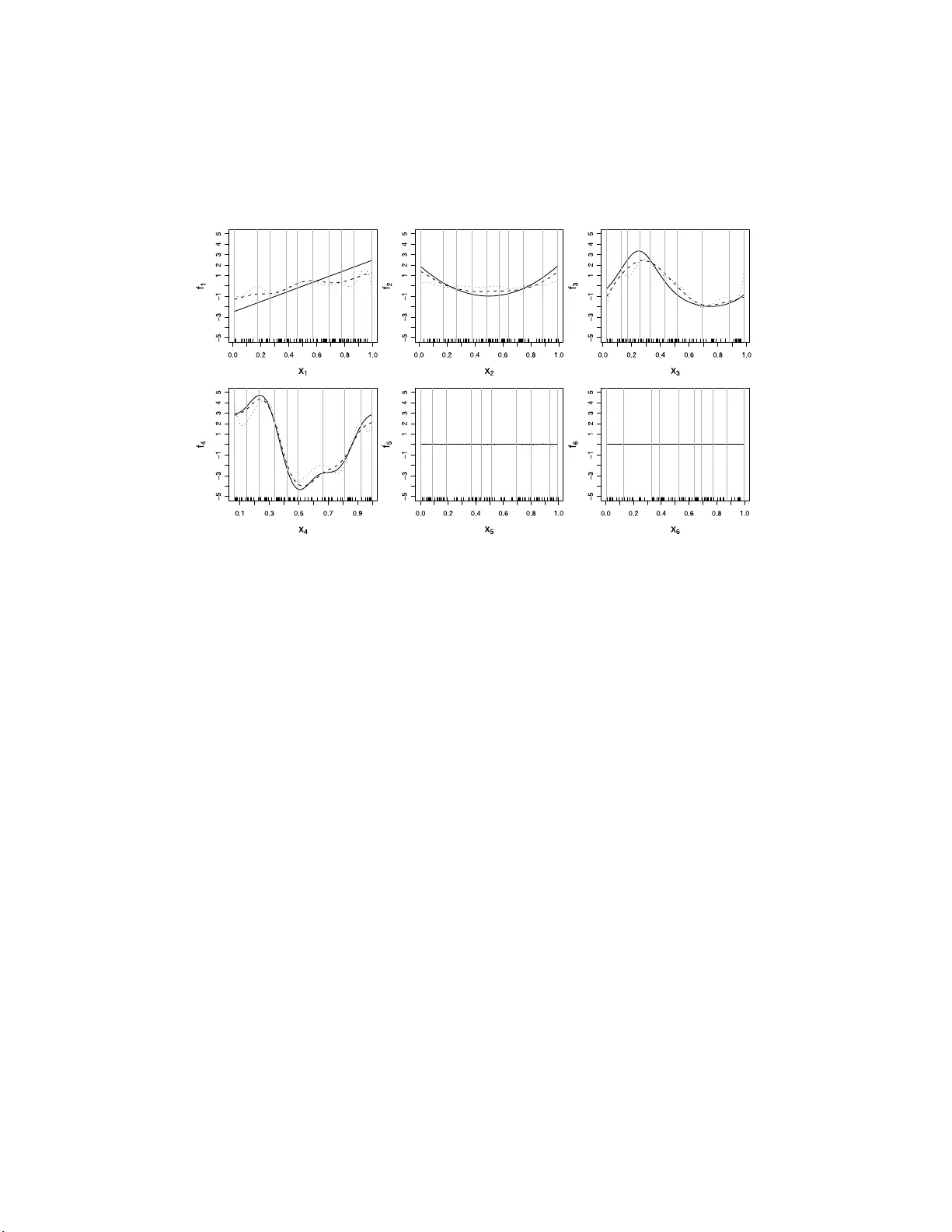
The Annals of Statistics 2009, V ol. 37, No. 6B, 3779–3 821 DOI: 10.1214 /09-A OS692 c  Institute of Mathematical Statistics , 2009 HIGH-DIMENSIONAL ADDITIVE MODELING By Lukas Meier, Sara v an de Geer and Peter B ¨ uhlmann ETH Z¨ urich W e prop ose a new sparsit y- smoothness penalty for high-d imen- sional g eneralized additiv e models. The com bination of sparsity and smoothness is crucia l for mathematical theory as w ell as p erformance for ﬁnite-sample data. W e present a computationally eﬃcien t algo- rithm, with pro va ble numerica l con verge nce properties, for optimizing the penalized likelihood . F urthermore, w e provide oracl e results which yield asymptotic optimality of our estimator for high dimensional but sparse additive mod els. Finally , an adaptive version of our sparsit y - smoothness p enalized approac h yields large additional p er formance gains. 1. In tro d uction. Substanti al prog ress has b een ac hiev ed o ver t he last y ears in estimating high-dimensional linear or generalized linea r models where the n umb er of co v ariates p is muc h larger than sample size n . The theoretica l prop erties o f p enalizati on approac hes lik e the lasso [ 28 ] are no w w ell u ndersto o d [ 3 , 14 , 23 , 24 , 33 ] and this kn owledge has led to sev eral extensions or alternati v e approac hes lik e adaptiv e la sso [ 34 ], relaxed lasso [ 22 ], sure in d ep endence screening [ 12 ] and graph ical mo d el based metho ds [ 6 ]. Moreo v er, with the fast gro wing amoun t of high-dimensional data in , for example, biolo gy , imaging or astronom y , t hese methods ha ve shown their success in a v ariet y of pr actica l problems. Ho w ever, in man y situations, the conditional exp ectati on of t he resp onse giv en the c o v ariates ma y not b e linear. While the most imp ortan t eﬀects ma y still b e d etected by a linear mo del, su bstan tial improv emen ts are somet imes possib le by using a more ﬂexible class of mo dels. Recent ly , some progress has b een made regarding high-dimensional additive mo del selection [ 7 , 19 , 26 ] and some theoretica l results are a v ailable [ 26 ]. Other approac hes are based on w a v elets [ 27 ] or can adapt t o th e u nkno wn smo othness of the u nderlying f unctions [ 2 ]. Received December 2008; rev ised F ebruary 2009. AMS 2000 subje ct cl assiﬁc ations. Primary 62G08, 62F1 2; secondary 62J07. Key wor ds and phr ases. Group lasso, model selection, nonparametric regression, oracle inequalit y, p en alized likelihoo d, sparsity. This is an electronic reprint of the or iginal article published by the Institute of Mathematical Statistics in The A nnals of Statistics , 2009, V ol. 37, No. 6B, 3779– 3821 . This reprint diﬀers from the orig inal in pagination and typog raphic detail. 1 2 L. MEIER, S. V AN DE GEER AN D P . B ¨ UHLMANN In this pap er, w e consider the p roblem of estimati ng a high-dimensional generalize d additiv e mo d el w here p ≫ n . An approac h for high-dimensional additiv e mo deling is describ ed and analyzed in [ 26 ]. W e use an approac h whic h p enalizes both the sp arsit y and the roughness. This is particularly imp ortan t if a large n u m b er of basis functions is used for modeling the ad- ditiv e co mp onents. This is similar to [ 26 ] where the smo othness and the sparsit y is con trolled in the bac kﬁ tting step. In add ition, our computational algorithm, wh ic h builds up on th e idea of a group lasso p roblem, has rigorous con ve rgence prop erties and th us, it is p ro v ably correct for ﬁ nding the opti- m u m of a p enaliz ed lik eliho o d function. Moreo v er, we provide oracl e results whic h establish asymptotic optimalit y of the procedur e. 2. P enalized maxim um lik eliho o d for additiv e mo dels. W e consider h igh- dimensional additiv e regression mo dels with a con tin uous resp onse Y ∈ R n and p co v ariates x (1) , . . . , x ( p ) ∈ R n connected through the mo del Y i = c + p X j =1 f j ( x ( j ) i ) + ε i , i = 1 , . . . , n, where c is the in tercept term, ε i are i.i.d. random v ariables w ith mean ze ro and f j : R → R are smo oth univ ariate functions. F or identi ﬁcation p urp ose s, w e assume that all f j are cen tered, that is, n X i =1 f j ( x ( j ) i ) = 0 for j = 1 , . . . , p . W e consider the case of ﬁxed design, that is, w e treat the predictors x (1) , . . . , x ( p ) as nonrand om. With some sligh t abuse of notation w e also denote by f j the n -dimensional v ector ( f j ( x ( j ) 1 ) , . . . , f j ( x ( j ) n )) T . F or a vec tor f ∈ R n , we deﬁne k f k 2 n = 1 n P n i =1 f 2 i . 2.1. The sp arsity-smo othness p enalty. In order to construct an estimator whic h encourages sparsit y at the function leve l, p enalizing the norms k f j k n w ould b e a suitable approac h . Some theory for the case where a truncated orthogonal basis with O ( n 1 / 5 ) basis functions for eac h comp onen t f j is used has b een dev elop ed in [ 26 ]. If w e use a large num b er of basis functio ns, whic h is necessary to be able to capture some functions at high complexit y , the resulting estimator will p ro duce function estimates whic h a re too wiggly if the underlying true functions are ve ry smo oth. Hence, w e need some additional con trol or restric- tions of the smo othn ess of the estimate d fu nctions. In order to get sp ars e and suﬃcien tly smo oth functio n estima tes, we propose the sparsit y-smo othness p enalt y J ( f j ) = λ 1 q k f j k 2 n + λ 2 I 2 ( f j ) , HIGH-DIMENSI ONAL ADDITIVE MODELING 3 where I 2 ( f j ) = Z ( f ′′ j ( x )) 2 dx measures the smo othness of f j . T he t w o tuning parameters λ 1 , λ 2 ≥ 0 con trol the a moun t o f p enaliza tion. Our estimator is giv en by the follo win g p enalized least squares p roblem: ˆ f 1 , . . . , ˆ f p = arg min f 1 ,...,f p ∈F      Y − p X j =1 f j      2 n + p X j =1 J ( f j ) , (1) where F is a suita ble class of functions and Y = ( Y 1 , . . . , Y n ) T is the vec tor of resp onses. W e assume the same lev el of regularit y for eac h fu nction f j . If Y is cente red, we can omit an un p enalized interce pt term and the nature of the ob jectiv e fun ction in ( 1 ) automatical ly forces the function estimat es ˆ f 1 , . . . , ˆ f p to b e cen tered. Pr oposition 1. L et a, b ∈ R such th at a < min i,j { x ( j ) i } and b > max i,j { x ( j ) i } . L et F b e the sp ac e of functions tha t a r e tw ic e c ont inuously diﬀer entiable on [ a, b ] and assume that ther e exist minimizers ˆ f j ∈ F of ( 1 ). Then the ˆ f j ’s ar e natur al cubic splines with knots at x ( j ) i , i = 1 , . . . , n . A pro of is giv en in App endix A . Hence, w e can r estrict ourselve s to the ﬁnite-dimensional space of natural cubic splines instead of considering the inﬁnite-dimensional spac e o f twice con tin u ous ly diﬀeren tiable f u nctions. In th e follo wing subs ection, w e ill ustrate t he exi stence and the computa- tion of the estimator. 2.2. Computatio nal algorithm. F or eac h function f j , w e u se a cub ic B- spline p arameteriza tion with a reaso nable amoun t of knots or basis func- tions. A t ypical c h oice w ould b e t o use K − 4 ≍ √ n in terior knots that are placed at the empirical quan tiles o f x ( j ) . Hence, w e parameterize f j ( x ) = K X k =1 β j,k b j,k ( x ) , where b j,k : R → R are the B-spline basis fu nctions and β j = ( β j, 1 , . . . , β j,K ) T ∈ R K is the parameter v ector corresp onding to f j . Based on the basis fu n c- tions, we can construct an n × pK design matrix B = [ B 1 | B 2 | · · · | B p ], w here B j is the n × K design matrix of the B-spline basis of the j th predictor, that is, B j,il = b j,l ( x ( j ) i ). 4 L. MEIER, S. V AN DE GEER AN D P . B ¨ UHLMANN F or t wice con tin uous ly diﬀeren tiable fun ctions, the optimization p roblem ( 1 ) ca n n o w b e reform ulated as ˆ β = arg min β =( β 1 ,...,β p ) k Y − B β k 2 n + λ 1 p X j =1 r 1 n β T j B T j B j β j + λ 2 β T j Ω j β j , (2) where the K × K matrix Ω j con tains the inner pro ducts of the second deriv a- tiv es of the B-spline basis functions, that is, Ω j,k l = Z b ′′ j,k ( x ) b ′′ j,l ( x ) dx for k, l ∈ { 1 , . . . , K } . Hence, ( 2 ) ca n b e rewritten a s a general group lasso problem [ 32 ] ˆ β = arg min β =( β 1 ,...,β p ) k Y − B β k 2 n + λ 1 p X j =1 q β T j M j β j , (3) where M j = 1 n B T j B j + λ 2 Ω j . By decomp osing (e.g., using the Cholesky de- comp osition) M j = R T j R j for some quadratic K × K matrix R j and b y deﬁning ˜ β j = R j β j , ˜ B j = B j R − 1 j , ( 3 ) red u ces to ˆ ˜ β = arg min ˜ β =( ˜ β 1 ,..., ˜ β p ) k Y − ˜ B ˜ β k 2 n + λ 1 p X j =1 k ˜ β j k , (4) where k ˜ β j k = √ K k ˜ β j k K is the Euclidean norm in R K . This is an ordinary group lasso pr oblem f or a n y ﬁxed λ 2 , a nd hence the existence of a solution is guaran teed. F or λ 1 large enough, some of the co eﬃcien t group s β j ∈ R K will b e estimated to b e exactly zero. Hence, the corresp ondin g functio n estimate will b e zero. Moreo ver, there exists a v alue λ 1 , max < ∞ such that ˆ ˜ β 1 = · · · = ˆ ˜ β p = 0 for λ 1 ≥ λ 1 , max . This is esp ecially u seful to construct a grid of λ 1 candidate v alues for cross-v alidatio n (usually o n th e log-scale). Regarding the un iqueness of the identiﬁed comp onen ts, we h a ve equiv alen t results as for the lasso. Deﬁne S ( ˜ β ; ˜ B ) = k Y − ˜ B ˜ β k 2 n . S imilar to [ 25 ], we ha v e the fo llo wing prop osition. Pr oposition 2. If pK ≤ n , and if ˜ B ha s ful l r ank, a unique sol ution of ( 4 ) exists. If pK > n , ther e exists a c onvex set of solutions of ( 4 ). Mor e- over, if k∇ ˜ β j S ( ˆ ˜ β ; ˜ B ) k < λ 1 , then ˆ ˜ β j = 0 and al l other solutions ˆ ˜ β other satisfy ˆ ˜ β other ,j = 0 . A pr o of can be foun d in App endix A . By rewriting the original pr oblem ( 1 ) in the form of ( 4 ), w e ca n mak e use of already existing algorithms [ 16 , 21 , 32 ] to compute the estimat or. HIGH-DIMENSI ONAL ADDITIVE MODELING 5 Fig. 1. T rue functions f j (solid) and estimate d functions ˆ f j (dashe d) for the ﬁrst 6 c om- p onents of a simulation run of Example 1 i n Se ction 3 . Smal l vertic al b ars indic ate original data and gr ey vert ic al lines knot p ositions. The dotte d l ines ar e the function estimates when no smo othness p enalty is use d, that is, when setting λ 2 = 0 . Co ordinate-wise appr oac hes as in [ 21 , 32 ] are eﬃcie n t and ha ve rigorous con ve rgence p rop erties. Th us, w e are able to compute the estimat or exactly , ev en if p is v ery large . An example of estimated functions, f rom s imulated dat a acco r ding to Example 1 in Secti on 3 , is sho wn in Figure 1 . F or illustrational pur p oses, w e ha ve also plotted the estimator whic h inv olv es no smo othness p enalt y ( λ 2 = 0). The latter clearly sho ws that for this example, the function estimates are “too wiggly” compared to the true functions. As w e will also see later, the smo othness penalt y pla ys a k ey role for the theory . Remark 1. Alternativ e p ossibilitie s of our p enalt y w ould b e to use ei- ther (i) J ( f j ) = λ 1 k f j k n + λ 2 I ( f j ) or (ii) J ( f j ) = λ 1 k f j k n + λ 2 I 2 ( f j ). Both approac hes lead to a sparse estimator. While prop osal (i) also enjo ys n ice theoretica l prop erties (see a lso Section 5.2 ), it is computationally more de- manding, b ecause it leads to a sec ond order co ne programming problem. Prop osal (ii) basically leads again to a group la sso problem, bu t app ears to ha v e theoretical dra wbac ks, that is, the term λ 2 I 2 ( f j ) is really needed within the square ro ot. 2.3. Or acle r esults. W e present now an oracle inequalit y for the p enalized estimator. Th e pr o ofs can b e found in App endix A . 6 L. MEIER, S. V AN DE GEER AN D P . B ¨ UHLMANN F or the theoretic al analysis, we in tro duce an add itional p enalt y parameter λ 3 ≥ 0 for tec hn ical rea sons. W e consider, here, a p enalt y of the form J ( f j ) = λ 1 q k f j k 2 n + λ 2 I 2 ( f j ) + λ 3 I 2 ( f j ) . This p enalt y in vo lv es three smoothing paramete rs λ 1 , λ 2 and λ 3 . One ma y reduce this to a single smo othing paramete r b y c ho osing λ 2 = λ 3 = λ 2 1 , (see T heorem 1 b elo w). In the sim ulations ho wev er, the c hoice λ 3 = 0 turned out to pro vide slig h tly b etter results than the c h oice λ 2 = λ 3 . W ith λ 3 = 0, the theory go es through provi ded the smo othness I ( ˆ f j ) remains b oun ded in an a ppropr iate s en s e. W e let f 0 denote the “true” regression function (whic h is not n ecessarily additiv e), that is, w e supp ose the reg ression model Y i = f 0 ( x i ) + ε i , where x i = ( x (1) i , . . . , x ( p ) i ) T for i = 1 , . . . , n , and where ε 1 , . . . , ε n are inde- p endent rand om errors with E [ ε i ] = 0. Let f ∗ b e a (sparse) additiv e approx- imation o f f 0 of the form f ∗ ( x i ) = c ∗ + p X j =1 f ∗ j ( x ( j ) i ) , where w e tak e c ∗ = E [ ¯ Y ] , ¯ Y = P n i =1 Y i /n . The r esu lt of this subsection (The- orem 1 ) h olds for any such f ∗ satisfying the compatibilit y conditio n b elo w. Th us, one ma y in v ok e the optimal additiv e predictor among such f ∗ , whic h w e will call the “oracle. ” F or an additiv e function f , the squared distance k f − f 0 k 2 n can b e decomp osed in to k f − f 0 k 2 n = k f − f 0 add k 2 n + k f 0 add − f 0 k 2 n , where f 0 add is the pro jectio n of f 0 on the space of additiv e functions. Thus, when f 0 is itself not add itiv e, the oracle can b e se en as the b est sparse appro ximation o f the pro jection f 0 add of f 0 . The active set is deﬁned as A ∗ = { j : k f ∗ j k n 6 = 0 } . (5) W e deﬁne, for j = 1 , . . . , p , τ 2 n ( f j ) = k f j k 2 n + λ 2 − γ I 2 ( f j ) . Moreo v er, w e let 0 < η < 1 b e some ﬁ xed v alue. The constan t 4 / (1 − η ) app earing b elo w in the compatibilit y condition is stated in this form to facilita te reference, la ter in the p ro of of Theorem 1 . HIGH-DIMENSI ONAL ADDITIVE MODELING 7 W e will use a compatibilit y condition, in the spirit of the inco herence conditions used for proving oracle inequalities for the standard lasso (see, e.g., [ 3 , 8 , 9 , 10 , 30 ]). T o av oid digressions, w e will not attempt to formula te the mo st g eneral cond ition. A discussion can be found in S ection 5.1 . Comp a tibility condition. F or some c onstan ts 0 < η < 1 and 0 < φ n, ∗ ≤ 1, and f or all { f j } p j =1 satisfying p X j =1 τ n ( f j ) ≤ 4 1 − η X j ∈A ∗ τ n ( f j ) , the fo llo wing inequalit y is met: X j ∈A ∗ k f j k 2 n ≤      p X j =1 f j      2 n + λ 2 − γ X j ∈A ∗ I 2 ( f j ) ! . φ 2 n, ∗ . F or practical app licatio ns, th e compatibilit y condition cannot b e c h eck ed b ecause the set A ∗ is unkno wn. Consider t he ge neral case wh ere I is some semi-norm, for example, as in Section 2.1 . F or mathemati cal con v enience, w e write f j = g j + h j (6) with g j and h j cen tered and orthogonal functions, that is, n X i =1 g j,i = n X i =1 h j,i = 0 and n X i =1 g j,i h j,i = 0 , suc h that I ( h j ) = 0 and I ( g j ) = I ( f j ). Th e functions h j are assumed to lie in a d -dimensional space. The en trop y of ( { g j : I ( g j ) = 1 } , k · k n ) is denoted b y H j ( · ); see, for e xample, [ 29 ]. W e assume that for all j , H j ( δ ) ≤ Aδ − 2(1 − α ) , δ > 0 , (7) where 0 < α < 1 and A > 0 are constan ts. When I 2 ( f j ) = R ( f ′′ j ( x )) 2 dx , the functions h j are th e linear p art of f j , that is, d = 1. Moreo v er, one then has α = 3 / 4 (see, e.g., [ 29 ], L emma 3.9). Finally , we assume sub-Gaussian tails for the errors: for some constan ts L and M , max i E [exp( ε 2 i /L )] ≤ M . (8) 8 L. MEIER, S. V AN DE GEER AN D P . B ¨ UHLMANN The n ext lemma presen ts the b eha vior of the empirical pr o cess. W e use the not ation ( ε, f ) n = 1 n P n i =1 ε i f ( x i ) f or the inner pro d uct. Deﬁne S = S 1 ∩ S 2 ∩ S 3 , (9) where S 1 =  max j sup g j  2 | ( ε, g j ) n | k g j k α n I 1 − α ( g j )  ≤ ξ n  , S 2 =  max j sup h j  2 | ( ε, h j ) n | k h j k n  ≤ ξ n  and S 3 = { ¯ ε ≤ ξ n } , ¯ ε = 1 n n X i =1 ε i . F or a n appropriate c hoice of ξ n , t he set S has la rge probabilit y . Lemma 1. Assume ( 7 ) and ( 8 ). Ther e exist c onstant s c and C dep ending only on d , α , A , L and M , such that for ξ n ≥ C s log p n , one has P ( S ) ≥ 1 − c exp[ − nξ 2 n /c 2 ] . F or α ∈ (0 , 1), w e deﬁne its “conjugate” γ = 2(1 − α ) / (2 − α ). Recall that when I 2 ( f j ) = R ( f ′′ j ( x )) 2 dx , one h as α = 3 / 4, and hence γ = 2 / 5. W e are no w ready to state the oracle result for ˆ f = ˆ c + P p j =1 ˆ f j as deﬁned in ( 1 ), with ˆ c = ¯ Y . Theorem 1. Supp ose the c omp atibility c ondition is met. T ake for j = 1 , . . . , p , J ( f j ) = λ 1 q k f j k 2 n + λ 2 I 2 ( f j ) + λ 3 I 2 ( f j ) with λ 1 = λ (2 − γ ) / 2 and λ 2 = λ 3 = λ 2 1 , and with ξ n √ 2 /η ≤ λ ≤ 1 . Then on th e set S given in ( 9 ), it hol ds that k ˆ f − f 0 add k 2 n + 2(1 − η ) λ (2 − γ ) / 2 p X j =1 τ n ( ˆ f j − f ∗ j ) + λ 2 − γ p X j =1 I 2 ( ˆ f j ) ≤ 3 k f ∗ − f 0 add k 2 n + 3 λ 2 − γ X j ∈A ∗  I 2 ( f ∗ j ) + 8 φ 2 n, ∗  + 2 ξ 2 n . HIGH-DIMENSI ONAL ADDITIVE MODELING 9 The result of Theorem 1 do es not dep en d on the n umber of knots (basis functions) whic h are used to build the functions ˆ f j , as long as ˆ f j and ˆ f ∗ j use the sa me basis fu nctions. W e wo uld like to p oin t out that the theory of Theorem 1 go es through with only t wo tuning p arameters λ 1 and λ 2 , b ut with the add itional restriction that I ( ˆ f j ) is appropriately b ounded. W e also remark that we did not attempt to op timize the constan ts giv en in Th eorem 1 , b ut rather look ed for a simple explicit boun d. Remark 2. Assume that φ n, ∗ is b oun ded a w a y fr om zero. F or example, this holds with la rge probabilit y for a realiz ation of a design with inde- p endent comp onen ts (see Section 5.1 ). In view of Lemma 1 , one may tak e (under the conditions of this lemma) th e smo othing parameter λ of ord er p log p/n . F or I 2 ( f j ) = R ( f ′′ j ( x )) 2 dx , γ = 2 / 5 and this giv es λ 2 − γ of order (log p/n ) 4 / 5 , which is up to the log-term the usual rate for estima ting a t wice diﬀeren tiable function. If the oracl e f ∗ has b ounded smo othness I ( f ∗ j ) for all j , Theorem 1 yields the con v ergence rate p act (log p/n ) 4 / 5 , with p act = |A ∗ | b eing the n umb er of activ e v ariables the oracle needs. This is again up to the log-te rm, the same rate one would obtain if it was kno wn b eforehand whic h of the p fu nctions are relev an t. F or general φ n, ∗ , we ha ve the con verge nce rate p act φ − 2 n, ∗ (log p/n ) 4 / 5 . F urthermore, the result implies that with large pr obabilit y , the estimator selects a sup-set of the activ e functions, pro vided that the latter hav e enough signal (suc h kin d of v ariable screening results ha v e b een esta blished for the lasso in linear and generalize d linear models [ 24 , 30 ]). More precise ly , w e ha ve the follo wing co rollary . Corollar y 1. L et A 0 = { j : k f 0 add ,j k n 6 = 0 } b e t he active s et of f 0 add . Assume the c omp atibility c onditio n holds for A 0 , with c onstant φ n, 0 . Supp ose also tha t for j ∈ A 0 , the sm o othness is b ounde d, say I ( f 0 add ,j ) ≤ 1 . Cho osing f ∗ = f 0 add in The or e m 1 , tel ls us that o n S , p X j =1 k ˆ f j − f 0 add ,j k n ≤ C λ (2 − γ ) / 2 |A 0 | /φ 2 n, 0 + 2 ξ 2 n for some c onstant C . Henc e, if k f 0 add ,j k n > C λ (2 − γ ) / 2 |A 0 | /φ 2 n, 0 + 2 ξ 2 n , j ∈ A 0 , we have (on S ), that the estimat e d active set { j : k ˆ f j k n 6 = 0 } c ontains A 0 . 10 L. MEIER, S. V AN DE GEER AN D P . B ¨ UHLMANN 2.4. Comp arison with r elate d r esults. After an earlier v ersion of this pa- p er, simila r results hav e b een pub lish ed in [ 17 ]. He re, w e p oin t out some diﬀerences and similarities b et w een o ur w ork and [ 17 ]. In [ 17 ], the framew ork of r epro ducing k ernel hilb ert spaces (RKHS) is considered, as for example, used in COSSO [ 19 ], while w e use p enalties based on smo othness seminorms. Hence, t he t wo framew orks are rather diﬀeren t, at least from a mathematical point of view. The resu lts in [ 17 ] a re v alid fo r a large class of loss functions, although w e w ould lik e to point out that the quadratic loss as studied here is not co ve red in [ 17 ] since t hey assume th at the l oss function is appropriately b ounded. The oracle result and the conditions in [ 17 ] are similar to our Theorem 1 . Regarding the co n v ergence rat e (see Remark 2 ), the rates obtained in [ 17 ] are s imilar in spirit to ours . In [ 17 ], the rate is slo w er than ours if the “smo othness” β is equal to 2. Moreo v er, “smo othn ess” in [ 17 ] i s very muc h in tertwined with the u nkno wn distribution of the co v ariabl es, whereas in our w ork “smo othness” is d eﬁned, for exa mple, in terms o f Sobolev-norms. Compared to th e w ork in [ 17 ], and, f or example, C OSSO [ 19 ], we gain ﬂexibilit y through the in tro duction of the additional p enal t y p arameter λ 2 for (separately) con trolling the sm o othness. In addition, w e presen t an al- gorithm in Section 2.2 whic h is eﬃcient with mathematicall y esta blished con ve rgence results. 3. Numerical examples. 3.1. Simulations. In this secti on, we in ve stigate the empirical pr op erties of the prop osed estimator. W e compare our approac h w ith the b o osting approac h of [ 7 ], where smo othing splines with lo w degrees of freedom are used as base learners; see a lso [ 5 ]. F or p = 1, b oosting with sp lines is kno wn to b e able to adapt to the smo othness of the underlying tru e f unction [ 7 ]. Generally , b o osting is a v ery p ow erful mac hine learning metho d and a wide v ariet y of soft w are implemen tations are av ailable, for exa mple, the R add-on pac k age mboost . W e use a trai ning set o f n samples to train the diﬀerent m etho ds. An indep end en t v alidatio n s et of size ⌊ n/ 2 ⌋ is used to select the prediction optimal tuning p arameters λ 1 and λ 2 . W e use grid s (on the log-scale) for b oth λ 1 and λ 2 , where the grid for λ 1 is of size 100 and the grid for λ 2 is t ypically of ab out size 15. F or b oosting, the num b er of b o osting iterations is used as tu ning paramete r. The shrink age facto r ν and the degrees of freedom d f of the bo osting pr o cedure are set to t heir d efault v alues ν = 0 . 1 and d f = 4 ; se e a lso [ 5 ]. By S NR, we denote the signal-to-noise ratio, wh ich is d eﬁ n ed as SNR = V ar( f ( X )) V ar( ε ) , HIGH-DIMENSI ONAL ADDITIVE MODELING 11 where f = f 0 : R p → R is the true und erlying function. A total of 100 simulat ion run s are u sed f or e ac h of the follo w ing settings. 3.1.1. Mo dels. W e use the follo wing sim ulation mod els. Example 1 ( n = 150, p = 200, p act = 4, SNR ≈ 15). This example is similar to Example 1 in [ 26 ] and [ 15 ]. Th e mo d el is Y i = f 1 ( x (1) i ) + f 2 ( x (2) i ) + f 3 ( x (3) i ) + f 4 ( x (4) i ) + ε i , ε i i.i.d. N (0 , 1) , with f 1 ( x ) = − sin(2 x ) , f 2 ( x ) = x 2 2 − 25 / 12 , f 3 ( x ) = x, f 4 ( x ) = e − x − 2 / 5 · sinh(5 / 2) . The co v ariates are simulate d from indep end ent Uniform( − 2 . 5 , 2 . 5) distribu- tions. The true and the estimated functions of a simula tion run are illus- trated in Figure 1 . Example 2 ( n = 100, p = 100 0, p act = 4, SNR ≈ 6 . 7). As ab o v e but high dimensional and correlated. T he co v ariates are sim u lated according to a m u ltiv ariat e normal distribution with co v ariance matrix Σ ij = 0 . 5 | i − j | ; i, j = 1 , . . . , p . Example 3 [ n = 100, p = 80, p act = 4, SNR ≈ 9 ( t = 0), ≈ 7 . 9 ( t = 1)]. This is similar to Example 1 in [ 19 ] b ut with mo re predictors. The mo del is Y i = 5 f 1 ( x (1) i ) + 3 f 2 ( x (2) i ) + 4 f 3 ( x (3) i ) + 6 f 4 ( x (4) i ) + ε i , ε i i.i.d. N (0 , 1 . 74) , with f 1 ( x ) = x, f 2 ( x ) = (2 x − 1) 2 , f 3 ( x ) = sin(2 π x ) 2 − sin(2 π x ) and f 4 ( x ) = 0 . 1 sin(2 π x ) + 0 . 2 cos (2 π x ) + 0 . 3 sin 2 (2 π x ) + 0 . 4 cos 3 (2 π x ) + 0 . 5 sin 3 (2 π x ) . The cov ariates x = ( x (1) , . . . , x ( p ) ) T are simula ted a ccording to x ( j ) = W ( j ) + tU 1 + t , j = 1 , . . . , p, where W (1) , . . . , W ( p ) and U are i.i.d. Uniform (0 , 1). F or t = 0 t his is the indep end en t uniform case. Th e case t = 1 resu lts in a design w ith correlation 0.5 bet w een a ll cov ariates. 12 L. MEIER, S. V AN DE GEER AN D P . B ¨ UHLMANN Fig. 2. T rue functions f j (solid) and es timate d functions ˆ f j (dashe d) for the ﬁrst 6 c omp onents of a simulation run of Example 3 ( t = 0 ). Smal l ver tic al b ars indic ate original data and gr ey vertic al lines knot p ositions. The dotte d lines ar e the function estimates when no smo othness p enalty i s use d, that is, when setting λ 2 = 0 . The true functions and the ﬁrst 6 estimated fun ctions of a sim u lation run with t = 0 are illustrated in Figure 2 . Moreo v er, w e a lso c onsider a “ high-frequency” situation where w e use f 3 (8 x ) and f 4 (4 x ) instead of f 3 ( x ) and f 4 ( x ). Th e corresp ond in g signal- to-noise ratios for these mo dels are SNR ≈ 9 for t = 0 a nd S NR ≈ 8 . 1 for t = 1. Example 4 [ n = 100, p = 60, p act = 12, SNR ≈ 9 ( t = 0), ≈ 11 . 25 ( t = 1)]. This is similar to Example 2 in [ 19 ] but with fewer observ ati ons. W e use the same f u nctions as in Example 3 . T he mo d el is Y i = f 1 ( x (1) i ) + f 2 ( x (2) i ) + f 3 ( x (3) i ) + f 4 ( x (4) i ) + 1 . 5 f 1 ( x (5) i ) + 1 . 5 f 2 ( x (6) i ) + 1 . 5 f 3 ( x (7) i ) + 1 . 5 f 4 ( x (8) i ) + 2 f 1 ( x (9) i ) + 2 f 2 ( x (10) i ) + 2 f 3 ( x (11) i ) + 2 f 4 ( x (12) i ) + ε i with ε i i.i.d. N (0 , 0 . 5184). The cov ariates are simulat ed as in Exa mple 3 . 3.1.2. Performanc e me asur es. In order to compare the pred iction per- formances, we use the mean squared prediction error PE = E X [( ˆ f ( X ) − f ( X )) 2 ] HIGH-DIMENSI ONAL ADDITIVE MODELING 13 T able 1 R esults of the diﬀer ent simulation mo dels. R ep orte d is the me an of the r atio of the pr e diction err or of the two metho ds. SSP: sp arsity-smo othn ess p enalty appr o ach, b o ost: b o osting with smo othing splines. Standar d deviations ar e given in p ar entheses Mod e l PE SSP / PE bo o st Example 1 0.93 (0.13 ) Example 2 0.96 (0.10) Example 3 ( t = 0) 0.81 (0.13 ) Example 3 ( t = 1) 0.90 (0.19 ) Example 3 “high-freq” ( t = 0) 0.65 (0.11 ) Example 3 “high-freq” ( t = 1) 0.57 (0.10 ) Example 4 ( t = 0) 0.89 (0.10 ) Example 4 ( t = 1) 0.88 (0.13 ) as p erf ormance measure. Th e ab o v e exp ecta tion is app ro ximated by a sample of 1 0,000 p oin ts from the distribution of X . In eac h simulat ion run, w e compute the ratio of the p rediction p erformance of the t wo metho ds. Finally , w e tak e the mean of the rat ios o v er all simulati on runs. F or v ariable select ion prop ertie s, w e u se the num b er o f true p ositiv es (TP) and false p ositiv es (FP) at eac h simulatio n run . W e rep ort the a v erage n um b er ov er all runs to compare the diﬀeren t metho ds. 3.1.3. R esults. The r esults are summarized in T ables 1 and 2 . The sparsity- smo othness p en alty approac h (SS P) has smaller prediction error than b o ost- ing, esp ecia lly for the “high-frequency” situations. Because the w eak learners of the b oosting metho d only use 4 d egrees of freedom, b oosting tends to ne- glect or underestimate those comp onents w ith higher oscillation. Th is can also b e observ ed with resp ect to the n u m b er of true p ositiv es. By relax- ing the smoothn ess penalt y (i.e., c ho osing λ 2 small or s etting λ 2 = 0), S SP is able to handle the h igh-frequency situati ons, at the cost of too wiggly function estimates for the remaining comp onent s. Usi ng a diﬀeren t a mount of regularization f or sparsit y and smo othness, SS P can work with a large amoun t of b asis functions in o rder to b e ﬂexible enough to c apture sophis- ticate d functional relationships and, on the other side, to p ro duce smo oth estimates if the un d erlying functions are smo oth. With the exception of the h igh-frequency examples, the num b er of true p ositiv es (TP ) is v ery similar for b oth metho ds. There is no clea r trend with resp ect to the num b er of false p ositiv es (FP). 3.2. R e al d ata. In this section, w e w ould lik e to compare the diﬀeren t estimators on real data sets. 14 L. MEIER, S. V AN DE GEER AN D P . B ¨ UHLMANN 3.2.1. T e c ator. The me atspec d ata set con tains data from the T ecator Infratec F o o d and F eed Analyzer. It is, for example, a v ailable i n the R add - on pac k age fara way and on StatLib. The p = 100 predictors are c hannel sp ectrum m easur emen ts, and are therefore highly correlated. A total of n = 215 observ ati ons are a v ailable. The data is split int o a trai ning s et of size 100 and a v alidation s et of size 50. Th e remaining d ata are used as test set. On the training dataset, the ﬁr s t 30 principal comp onents are ca lculated, scaled to unit v ariance and used as co v ariates in additiv e mo deling. Moreo ver, the v alidation and test data sets are transform ed to corresp on d to the principal comp onents of the training data set. W e ﬁt an additive m o del to pred ict the logarithm of the fat con tent . This is rep eated 50 times. F or eac h split into training and test d ata, w e c ompute the ratio of the prediction err ors fr om the SSP and b o osting metho d on the test data, as in S ection 3.1.2 . The mean of the ratio ov er the 50 splits is 0.8 6, the corresp ond ing standard deviati on is 0.46. This indicates sup eriority of our spars ity-smoothness penalty approac h . 3.2.2. Motif r e gr ession. In motif regression pr oblems [ 11 ], the aim is to predict gene expression lev els or binding intensitie s based on informa- tion on the DNA sequence. F or our sp eciﬁc dataset, from the Ricci lab at ETH Zurich, we ha v e binding inte nsities Y i of a certain transcription f actor (TF) at 287 regions on the DNA. Moreo v er, for eac h region i , motif scores x (1) i , . . . , x ( p ) i , p = 196 are av ailable. A motif is a candidate for the binding site of th e TF on the DNA, typica lly a 5–15bp long DNA sequence. T he score x ( j ) i measures how w ell the j th motif is r epresen ted in the i th r egion. Th e candidate list of mo tifs and their corresp onding scores w ere create d w ith a v arian t of the MD Scan alg orithm [ 20 ]. The main goal here is to ﬁnd the relev an t co v ariates. T able 2 Av er age values of the numb er of true ( TP ) and f alse ( FP ) p ositives. Standar d deviations ar e given in p ar entheses Mod e l TP SSP FP SSP TP bo o st FP bo o st Example 1 4 . 00 (0.00) 24 . 30 (14.11 ) 4 . 00 (0.00 ) 22 . 18 ( 12.75) Example 2 3 . 47 (0.61) 34 . 37 (17.38) 3 . 60 (0.64) 28 . 76 (20.1 5) Example 3 ( t = 0) 4 . 00 (0.00) 20 . 20 (9.30) 4 . 00 (0.00 ) 21 . 61 ( 10.90) Example 3 ( t = 1) 3 . 93 (0.29) 19 . 28 (9.61) 3 . 92 (0.27 ) 18 . 65 ( 8.35) Example 3 “high-freq” ( t = 0) 2 . 80 (0.78) 12 . 26 (7.61) 2 . 16 (0.94) 9 . 23 (9.74) Example 3 “high-freq” ( t = 1) 2 . 46 (0.85) 11 . 17 (8.50) 1 . 59 (1.27) 13 . 24 (13.89 ) Example 4 ( t = 0) 11 . 69 (0.56) 21 . 23 (6.85 ) 11 . 68 ( 0.57) 25 . 91 (9.43) Example 4 ( t = 1) 10 . 64 (1.15) 19 . 78 (7.51 ) 10 . 67 ( 1.25) 23 . 76 (9.89) HIGH-DIMENSI ONAL ADDITIVE MODELING 15 Fig. 3. Estimate d functions ˆ f j of the two most stable motifs. Smal l vertic al b ar i ndic ate original data. W e used 5 fold c ross-v alidatio n to dete rmine the pred iction optimal tun- ing parameters, yielding 28 activ e functions. T o assess the stabilit y of the estimated mo del, we p erformed a nonparametric b ootstrap analysi s. At eac h of the 100 b o otstrap samples, w e ﬁt the mo del w ith th e ﬁx ed optimal tuning parameters from ab o ve. The t w o fun ctions whic h app ear most often in the b o otstrapp ed m o del estimates are depicted in Figure 3 . While the left-hand side p lot sho ws an approximat e linear relationship, the eﬀect of th e other motif se ems to diminish for large r v alues. Indeed, M otif.P1. 6.26 is the true (kno wn) b inding site. A follo w-up exp eriment sh o wed that the TF do es not direct ly bind to M otif.P1. 6.23 . Hence, this motif is a candidate for a binding site of a co-factor (another TF) and needs fu r ther exp erimen tal v alidatio n. 4. Extensions. 4.1. Gener alize d add itive mo dels. Conceptually , we can also apply the sparsit y-smo othness p enalt y f r om Section 2 to generalize d linear mo dels (GLM) by replacing the residual su m of squares k Y − P p j =1 f j k 2 n b y the corresp onding negativ e log-lik elihoo d fun ction. W e illustrate the metho d for logistic regression where Y ∈ { 0 , 1 } . The negativ e log-l ik eliho o d as a function of t he linear predictor η and the resp onse v ector Y is ℓ ( η , Y ) = − 1 n n X i =1 [ Y i η i − log { 1 + exp( η i ) } ] , 16 L. MEIER, S. V AN DE GEER AN D P . B ¨ UHLMANN T able 3 R esults of diﬀer ent mo del sizes p . Re p orte d is the me an of the r atio of the pr e diction err or of the two metho ds. SSP: sp arsity-smo othnes s p enalty appr o ach, b o ost: b o osting with smo othing splines. Standar d deviations ar e given i n p ar entheses p PE SSP / PE bo o st 250 0.93 (0.06) 500 0.96 (0.07) 1000 0.98 (0.05) where η i = c + P p j =1 f j ( x ( j ) i ). The estimator is deﬁned as ˆ c, ˆ f 1 , . . . , ˆ f p = arg min c ∈ R ,f 1 ,...,f p ∈F ℓ c + p X j =1 f j , Y ! + p X j =1 J ( f j ) . (10) This has a simila r f orm as ( 1 ) with t he exception that w e hav e to explicitly include a (nonpenalized) in tercept term c . Using the same arguments as in Section 2 , leads to the fact that for t wice con tin uous ly diﬀeren tiable func- tions, the solution can b e represen ted as a natural cubic spline and that ( 10 ) leads again to a g roup lasso problem. This can, for exa mple, b e minimized with the algorithm of [ 21 ]. W e illustrate the p erformance of the estimator in a small simulat ion study . 4.1.1. Smal l simula tion study. Denote by f : R p → R the true fu n ction of Exa mple 2 in Section 3 . W e sim ulate the th e linear predictor η as η ( X ) = 1 . 5 · (2 + f ( X )) , where X ∈ R p has the same distribution as in Examp le 2 . T he b inary r e- sp onse Y is then generated according to a Bernoulli distribution with pr ob- abilit y 1 / (1 + exp( − η ( X )), whic h results in a Ba ye s risk of appr o ximately 0.17. The sample size n is set to 100. Th e results for v arious mo del sizes p are rep orted in T ables 3 and 4 . The p erformance of the tw o m etho ds is qu ite similar. SSP h as a s lightly low er p rediction error. Regarding mo del select ion prop erties, SS P has fewer false p ositiv es at the cost of slightl y fewer tru e p ositiv es. 4.2. A daptivity. Similar to the adaptiv e lasso [ 34 ], w e can also u se dif- feren t p enalti es for the d iﬀeren t comp onen ts, that is, use a p enalt y of the form J ( f j ) = λ 1 q w 1 ,j k f j k 2 n + λ 2 w 2 ,j I 2 ( f j ) , HIGH-DIMENSI ONAL ADDITIVE MODELING 17 where the we igh ts w 1 ,j and w 2 ,j are ideally c hosen in a data-adaptiv e wa y . If an initial estimator ˆ f j, init is a v aila ble, a choic e w ould b e to use w 1 ,j = 1 k ˆ f j, init k γ n , w 2 ,j = 1 I ( ˆ f j, init ) γ for some γ > 0 . Th e estima tor c an then b e computed s imilarly as d escrib ed in Section 2.2 . T his allo ws f or diﬀerent degrees of smo othness for diﬀerent comp onen ts. W e ha ve applied t he adaptiv e estimator to t he simulatio n models of Sec- tion 3 . In eac h simulat ion run , we use w eigh ts (with γ = 1 ) based on the ordi- nary sparsit y-smo othness estimator. F or comparison, w e compute the ratio of the p rediction error of the adaptiv e and the ord inary sparsit y-smo othness estimator at eac h simulat ion run. The results are summ arized in T able 5 . Both the pr ediction error and the num b er of false p ositiv es can b e decreased b y a goo d m argin in all examples. The n umb er of true p ositiv es gets sligh tly decreased in some examples. 5. Mathematic al theory . T able 4 Av er age values of the numb er of true ( TP ) and f alse ( FP ) p ositives. Standar d deviations ar e given in p ar entheses p TP SSP FP SSP TP bo o st FP bo o st 250 2.94 (0.71 ) 22.81 (10.56) 3.09 (0.78) 29.67 (14.9 1) 500 2.56 (0.82 ) 24.92 (12.47) 2.80 (0.82) 31.41 (17.2 8) 1000 2.36 (0.84) 26.45 (14.8 8) 2.61 (0.71) 33.69 (19.54 ) T able 5 R esults of the diﬀer ent simulation mo dels. R ep orte d is the me an of the r atio of the pr e diction err or of the two metho ds and the aver age values of the numb er of true ( TP ) and false ( FP ) p ositives. SSP; adapt: adaptive sp arsity-smo othness p enalty appr o ach, SSP: or di nary sp arsity-smo othnes s p enalty appr o ach. Standar d deviations ar e given i n p ar entheses Mod e l PE SSP; adapt / PE SSP TP FP Example 1 0.47 (0.13 ) 4.00 (0.00 ) 4.09 (4.63 ) Example 2 0.63 (0.17) 3 .31 (0.71) 6 .12 (5.14) Example 3 ( t = 0) 0.53 (0.14 ) 4.00 (0.00 ) 4.64 (4.52 ) Example 3 ( t = 1) 0.63 (0.22 ) 3.81 (0.46 ) 5.04 (4.82 ) Example 3 “high-freq” ( t = 0) 0.87 (0.09 ) 2.28 (0.78 ) 2.98 (2.76 ) Example 3 “high-freq” ( t = 1) 0.91 (0.10 ) 1.69 (0.73 ) 2.59 (3.30 ) Example 4 ( t = 0) 0.77 (0.11 ) 11.21 (0.84) 8.1 8 (5.04) Example 4 ( t = 1) 0.88 (0.12 ) 9.73 (1.29 ) 7.93 (5.35 ) 18 L. MEIER, S. V AN DE GEER AN D P . B ¨ UHLMANN 5.1. On the c omp atibility c ondition. W e sh o w in this subsection that the compatibilit y condition h olds un der reasonable co nditions when I ( f j ) = s Z 1 0 | f ( s ) ( x ) | 2 dx is the Sob olev norm ( f ( s ) j b eing the s th deriv ativ e of f j ), and wh en in ad- dition, the X i = ( X (1) i , . . . , X ( p ) i ) are i.i.d. copies of a p -dimensional random v ariable X ∈ [0 , 1] p with distrib ution Q . Then, the compatibilit y condition ma y b e r ep laced b y a theoretical v arian t, where the norm k · k n is replaced b y the theoretica l L 2 ( Q )-norm k · k . The theoretical compatibilit y condi- tion (giv en b elo w) is not ab out n -dimensional ve ctors, bu t ab out fun ctions. In that se nse, the sa mple size n pla ys a less p rominen t role . F or exam- ple, the theoretical compati bilit y condition is satisﬁed when the comp onents X (1) , . . . , X ( p ) are indep enden t. The main assumption to mak e the replacemen t b y a theoretical ve rsion p ossible, is the requirement that λ 1 − γ |A ∗ | [with γ = 2 / (2 s + 1)] is small in an appropriate sense [see ( 11 )]. T his i s comparable to the condition λ |A ∗ | b eing small, for the ordinary lasso (see, e.g., [ 9 ]). In fact, our app roac h for the transition from ﬁxed to r andom d esign ma y also shed new ligh t on the same transition for the lasso. Let X = ( X (1) , . . . , X ( p ) ∈ [0 , 1] p ha ve distribution Q , and let X 1 , . . . , X n b e i.i.d. copies of X . T he marginal d istribution of X ( j ) is den oted by Q j . W e write k f k 2 = Z f 2 dQ and f or a fun ction f j dep endin g only on the j th v ariable X ( j ) , k f j k 2 = Z f 2 j dQ j . In th is sub section, we assume all f j ’s are cen tered: Z f j dQ j = 0 , j = 1 , . . . , p. Recall the notation τ 2 n ( f j ) = k f j k 2 n + λ 2 − γ I 2 ( f j ) . W e now also deﬁne the theoreti cal coun terparts τ 2 ( f j ) = k f j k 2 + λ 2 − γ I 2 ( f j ) HIGH-DIMENSI ONAL ADDITIVE MODELING 19 and w rite τ tot ( f ) = τ in ( f ) + τ out ( f ) , τ in ( f ) = X j ∈A ∗ τ ( f j ) , τ out ( f ) = X j / ∈A ∗ τ ( f j ) . One now ma y actually redress the pro ofs for the oracle inequalit y directly , in order to hand le random design. T his will generally lead to b etter constan ts as the a pproac h that w e no w tak e, whic h is s h o win g that the co nditions for ﬁxed design h old with large probabilit y . The adv an tage of this detour is ho wev er that we do not ha ve to repeat the main bo dy of the pro of. The th eoretical compatibilit y conditio n is of the same form as the empir- ical on e, but with diﬀeren t c onstan ts. Theoretical comp a tibility condition. F or a constant 0 < η < 1 and 0 < φ ∗ ≤ 1, and f or all f sati sfying τ tot ( f ) ≤ c η τ in ( f ) , where c η = 4(1 + η ) (1 − η ) 2 , w e ha ve X j ∈A ∗ k f j k 2 ≤  k f k 2 + λ 2 − γ X j ∈A ∗ I 2 ( f j )  . φ 2 ∗ . Note that the theoretical compatibilit y condition trivially holds when the comp onen ts of X are ind ep enden t. Ho wev er, ind ep endence is n ot a necessary condition: m uc h broader schemes are all o wed. Let C 0 b e a constan t and S 4 =  sup f |k f k 2 n − k f k 2 | τ 2 tot ( f ) ≤ C 0 λ 1 − γ  . In App endix B , we sho w that for an appropriate v alue o f λ , S 4 has large probabilit y , for a constan t C 0 dep endin g only on s , and on an assumed lo wer b ound for the marginal densities of the X ( j ) . In fact, it turns out that one can tak e λ of order p log p/n und er w eak conditions, assuming I ( · ) is the Sob olev norm. Theorem 2. Assume 2 C 0 c 2 η |A ∗ | λ 1 − γ φ 2 ∗ ≤ 1 . (11) 20 L. MEIER, S. V AN DE GEER AN D P . B ¨ UHLMANN Then on S 4 , the the or e tic al c omp atibility c ondition implies the empiric al one as given in Se ction 2.3 , with c onstant 1 φ 2 n, ∗ =  (1 + η )(1 + φ 2 ∗ ) + 2(1 + η ) φ 2 ∗ + η  . As previously mentio ned, condition ( 11 ) implies that the n umb er of activ e comp onen ts c annot g ro w to o fast in ord er for |A ∗ | λ 1 − γ b eing s mall. W e no w h a ve a quick closer lo ok at the theoretical compatibilit y condi- tion. The follo wing t wo conditions are su ﬃcien t and migh t yield some more insigh t. Well-conditione d active set condition. W e sa y that the activ e set A ∗ is w ell conditioned if for some constan t 0 < ψ ∗ ≤ 1, and for all { f j } j ∈A ∗ , X j ∈A ∗ k f j k 2 ≤     X j ∈A ∗ f j     2 . ψ 2 ∗ . The inner prod uct in L 2 ( Q ) b et w een fu n ctions f and ˜ f is denoted b y ( f , ˜ f ). No p erfect canonical d ep endence in our setup amounts to the follo w- ing c ondition. No p erfect can onical depende nce condition. W e s ay that t he activ e and nonactiv e v ariables ha ve no p erfect canonical d ep endence, if for a constan t 0 ≤ ρ ∗ < 1, and all { f j } p j =1 , w e h a ve for f in = P j ∈A ∗ f j and f out = P j / ∈A ∗ f j , t hat | ( f in , f out ) | k f in kk f out k ≤ ρ ∗ . The next lemma mak es the link b et wee n the theoretical compatibilit y condition and the ab o v e t wo conditions. Lemma 2. L et f = f in + f out satisfy | ( f in , f out ) | k f in kk f out k ≤ ρ ∗ < 1 . Then k f in k 2 ≤ k f k 2 / (1 − ρ 2 ∗ ) . HIGH-DIMENSI ONAL ADDITIVE MODELING 21 Pr oof. Clea rly , k f in k 2 ≤ k f k 2 + 2 | ( f in , f out ) | − k f out k 2 . Hence, k f in k 2 ≤ k f k 2 + 2 ρ ∗ k f in kk f out k − k f out k 2 ≤ k f k 2 + ρ 2 ∗ k f in k 2 .  Corollar y 2. A wel l-c onditio ne d active set in c ombination with no p erfe ct c anonic al dep endenc e implies the the or etic al c omp atibility c ondition with φ 2 ∗ = ψ 2 ∗ (1 − ρ 2 ∗ ) . Remark 3 . Canonica l dep endence is ab out the d ep endence stru cture of v ariables. T o compare, let X in and X out b e t wo r andom v ariables, with join t density q , and with marginal densities q in and q out . De ﬁne for r eal- v alued measurable fu nctions f in and f out , of X in and X out , resp ectiv ely , the squared norms k f in k 2 = R f 2 in q in , and k f out k 2 = R f 2 out q out , and the in ner pro du ct ( f in , f out ) = R f in f out q . Assu me the functions are cente red: R f in q in = R f out q out = 0. Supp ose that for some constant ρ ∗ , Z q 2 q in q out ≤ 1 + ρ 2 ∗ . Then o ne ca n easily v erify that | ( f in , f out ) | ≤ ρ ∗ k f in kk f out k . In other words, the no p erfe ct c anonic al dep endenc e c ondition is in this con text th e assump- tion that the d ensit y and the p ro duct dens ity are, in χ 2 -sense, not to o far oﬀ. 5.2. On the choic e of the p enalty. In this pap er, w e ha v e c h osen the p enalt y in suc h a wa y that it lea ds to go o d theoretical b ehavi or (namely the oracle inequalit y of Theorem 1 ), as wel l as to computationally fast, and in fact already existi ng, algorithms. The p enalt y can b e imp ro ve d theoretically , at the cost of computatio nal eﬃcie ncy and simplicit y . Indeed, a main ingredient from the theoretical p oint of view is that the randomness of the problem (the b eha vior of the emp irical pro cess) should b e tak en care of. Let u s recall Lemma 1 w hic h sa ys that the set S has large probabilit y , and on S all functions g j satisfy ( ε, g j ) n ≤ ξ n k g j k α n I 1 − α ( g j ) . Our p enalt y was based on the inequalit y (whic h h olds for a n y a a nd b p osi- tiv e) a α b 1 − α ≤ p a 2 + b 2 . More generally , it holds for an y q ≥ 1 that a α b 1 − α ≤ ( a q + b q ) 1 /q . 22 L. MEIER, S. V AN DE GEER AN D P . B ¨ UHLMANN In particular, th e c hoice q = 1 would b e a natural one, and w ould lead to an oracle inequalit y in volving I ( f ∗ j ) instead of the square I 2 ( f ∗ j ) on the righ t- hand side in Theorem 1 . The p enalt y λ (2 − γ ) / 2 P p j =1 k f j k n + λ 2 − γ P p j =1 I ( f j ), corresp onding to q = 1, still in v olve s conv ex optimization b ut whic h is muc h more in v olved and hence less eﬃcie n t to b e solv ed; see also Remark 1 in Section 2.2 . One may also use th e in equalit y a α b 1 − α ≤ a 2 + b γ . This leads to a “theoretically i deal” p enalt y of th e from λ 2 − γ P p j =1 I γ ( f j ) + λ P p j =1 k h j k n , wh ere h j is from ( 6 ). It allo ws to adapt to small v alues of I ( f ∗ j ). But clearly , as this p enalt y is noncon v ex, it may b e computat ionally cum b ersome. On the other hand, iterativ e appr o ximations migh t p r o ve to w ork w ell. 6. Conclusions. W e present an estimator and algorithm for ﬁ tting sparse, high-dimensional generalized add itiv e mo dels. The estimator is based on a p enalized lik eliho o d. T h e penalt y is new, as it allo ws for diﬀeren t regu- larizatio n of the sparsit y and the smo othness of the add itiv e functions. It is exactly this com bination which allo w s to d erive oracle r esults for high- dimensional additiv e mo dels. W e also argue emp irically that the inclusion of a smo othness-part in to the p enalt y f u nction yields m uc h b etter results than ha ving the s p arsit y-term only . F u rthermore, w e show that the optimization of the p enalized lik eliho o d ca n b e written as a group l asso problem and hence, eﬃcient co ordinate-wise algorithms can b e used wh ic h ha ve pro v able n umerical conv ergence prop erties. W e illustrate some empirical results for sim ulated and real data. Our new approac h with the spars ity and s mo othness p enalt y is neve r worse and some- times su bstan tially b etter than L 2 -b o osting for generaliz ed additiv e mo del ﬁtting [ 5 , 7 ]. F urthermore, with an a daptiv e sparsit y-smo othness p enalt y metho d, large additional p erformance gains are ac h iev ed. With the real data ab out m otif regression for ﬁn ding DNA-sequence m otifs, one among t wo se- lected “stable” v ariables is kno wn to b e true, that is, it corresp onds to a kno wn binding site of a transcription factor. APPENDIX A: P R OO FS Pr oof of Pr opo sition 1 . B ecause of the additiv e str u cture of f and the p enalt y , it suﬃces to analyze eac h comp onen t f j , j = 1 , . . . , p ind ep en- den tly . L et ˆ f 1 , . . . , ˆ f p b e a solution of ( 1 ) and assume that some or all ˆ f j are not nat ural cub ic splines with knots at x ( j ) i , i = 1 , . . . , n . By Theorem 2.2 in HIGH-DIMENSI ONAL ADDITIVE MODELING 23 [ 13 ], w e can construct natural cubic splines ˆ g j with knots at x ( j ) i , i = 1 , . . . , n suc h that ˆ g j ( x ( j ) i ) = ˆ f j ( x ( j ) i ) for i = 1 , . . . , n and j = 1 , . . . , p . H ence,      Y − p X j =1 ˆ g j      2 n =      Y − p X j =1 ˆ f j      2 n and k ˆ g j k 2 n = k ˆ f j k 2 n . But b y Theorem 2.3, in [ 13 ], I 2 ( ˆ g j ) ≤ I 2 ( ˆ f j ). Therefore, the v alue in the ob jectiv e fun ction ( 1 ) can b e decreased. Hence, the minimizer of ( 1 ) must lie in the space of natural c ubic s p lines.  Pr oof of Proposition 2 . The ﬁ rst p art follo ws b ecause of the strict con ve xit y of t he ob jectiv e function. Consider no w the c ase p K > n . The (necessary and suﬃ cient) conditions for ˆ ˜ β to b e a solution of the group lasso problem ( 4 ) are [ 32 ] k∇ ˜ β j S ( ˆ ˜ β ; ˜ B ) k = λ 1 for ˆ ˜ β j 6 = 0 , k∇ ˜ β j S ( ˆ ˜ β ; ˜ B ) k ≤ λ 1 for ˆ ˜ β j = 0 . Assume that there exist tw o solutions ˆ ˜ β (1) and ˆ ˜ β (2) suc h that, for a comp o- nen t j , we hav e ˆ ˜ β (1) j = 0 with k∇ ˜ β j S ( ˆ ˜ β (1) ; ˜ B ) k < λ 1 , b ut ˆ ˜ β (2) j 6 = 0. Because the se t o f all solutions is con v ex, ˆ ˜ β ρ = (1 − ρ ) ˆ ˜ β (1) + ρ ˆ ˜ β (2) is also a minimiz er for al l ρ ∈ [0 , 1]. By assumption ˆ ˜ β ρ,j 6 = 0, and hence k∇ ˜ β j S ( ˆ ˜ β ρ ; ˜ B ) k = λ 1 for all ρ ∈ (0 , 1). Hence, it h olds for g ( ρ ) = k∇ ˜ β j S ( ˆ ˜ β ρ ; ˜ B ) k that g (0) < λ 1 and g ( ρ ) = λ 1 for all ρ ∈ (0 , 1). But this is a contradict ion to the f act that g ( · ) is con tin uous . Hence, a nonactiv e (i .e., zero) comp o- nen t j w ith k∇ ˜ β j S ( ˆ ˜ β ; ˜ B ) k < λ 1 cannot b e activ e ( i.e., nonzero) in any other solution.  Pro of of Lemma 1 . The result easily follo ws from Lemma 8.4 in [ 29 ], whic h w e cite here for completeness. 24 L. MEIER, S. V AN DE GEER AN D P . B ¨ UHLMANN Lemma 3. L et G b e a c ol le ction of functions g : { x 1 , . . . , x n } → R , en- dowe d with a metric induc e d by th e norm k g k n = ( 1 n P n i =1 g 2 ( x i )) 1 / 2 . L et H ( · ) b e the entr opy of G . Supp ose that H ( δ ) ≤ Aδ − 2(1 − α ) ∀ δ > 0 . F urthermor e, let ε 1 , . . . , ε n b e indep endent c enter e d r ando m v ariables, satis- fying max i E [exp( ε 2 i /L )] ≤ M . Then for a c onstant c 0 dep ending on α , A , L and M , we have for al l T ≥ c 0 , P  sup g ∈G | 2( ε, g ) n | k g k α n > T √ n  ≤ c 0 exp  − T 2 c 2 0  . Pr oof of Lemma 1 . It is clear that { g j /I ( g j ) } = { g j : I ( g j ) = 1 } . Hence, b y rewriting and then using Lemma 3 , sup g j | 2( ε, g j ) n | k g j k α n I 1 − α ( g j ) = su p g j | 2( ε, g j /I ( g j )) n | k g j /I ( g j ) k α n ≤ T √ n with probabilit y at least 1 − c 0 exp( − T 2 /c 2 0 ). T hus, for C 2 0 ≥ 2 c 2 0 suﬃcien tly large P max j sup g j | 2( ε, g j ) n | k g j k α n I 1 − α ( g j ) > C 0 s log p n ! ≤ pc 0 exp  − C 2 0 log p c 2 0  ≤ c 0 exp  − C 2 0 log p 2 c 2 0  . In the same spirit, for some constant c 1 dep endin g on L and M , it holds for all T ≥ c 1 , wit h probabilit y at least 1 − c 1 exp( − T 2 d/c 2 1 ), sup h j | 2( ε, h j ) n | k h j k n ≤ T s d n , where d is the dimension o ccurring in ( 6 ). This result is rather standard but also follo ws from th e more general Corollary 8.3 in [ 29 ]. I t yields that for C 2 1 ≥ 2 c 2 1 , dep ending on d , L a nd M , max j sup h j | 2( ε, h j ) n | k h j k n ≤ C 1 s log p n with p r obabilit y at least 1 − c 1 exp( − C 2 1 log p/ (2 c 2 1 )). HIGH-DIMENSI ONAL ADDITIVE MODELING 25 Finally , it is ob vious that for all C 2 and a constan t c 2 dep endin g on L and M , P ¯ ε > C 2 s log p n ! ≤ 2 exp( − C 2 2 log p/c 2 2 ) . Cho osing c 2 ≥ 2, t he resu lt n o w fo llo ws b y taking C = max { C 0 , C 1 , C 2 } and c = c 0 + c 1 + c 2 .  Pro of of Theorem 1 . W e b egin with t hree te c hn ical l emmas. Recall that (for j = 1 , . . . , p ) τ 2 n ( f j ) = k f j k 2 n + λ 2 − γ I 2 ( f j ) . Lemma 4. F or λ ≥ √ 2 ξ n /η , we have on S 1 ∩ S 2 , max j sup f j 2 | ( ǫ, f j ) | λ (2 − γ ) / 2 τ n ( f j ) ≤ η . Pr oof. No te ﬁrst that with λ ≥ √ 2 ξ n /η , ξ n k g j − g ∗ j k α n I 1 − α ( g j − g ∗ j ) + ξ n k h j − h ∗ j k n ≤ η λ √ 2 k g j − g ∗ j k α n I 1 − α ( g j − g ∗ j ) + η λ √ 2 k h j − h ∗ j k n ≤ η λ (2 − γ ) / 2 √ 2 q λ 2 − γ I 2 ( g j − g ∗ j ) + k g j − g ∗ j k 2 n + η λ √ 2 k h j − h ∗ j k n ≤ η λ (2 − γ ) / 2 √ 2 q λ 2 − γ I 2 ( g j − g ∗ j ) + k g j − g ∗ j k 2 n + η λ (2 − γ ) / 2 √ 2 k h j − h ∗ j k n , since λ ≤ 1. W e hav e q λ 2 − γ I 2 ( g j − g ∗ j ) + k g j − g ∗ j k 2 n + k h j − h ∗ j k n ≤ q 2 { λ 2 − γ I 2 ( g j − g ∗ j ) + k g j − g ∗ j k 2 n + k h j − h ∗ j k 2 n } = √ 2 q λ 2 − γ I 2 ( g j − g ∗ j ) + k f j − f ∗ j k 2 n , where w e used the orthogo nalit y of g j − g ∗ j and h j − h ∗ j . The result no w follo ws from th e equalit y I ( g j − g ∗ j ) = I ( f j − f ∗ j ).  26 L. MEIER, S. V AN DE GEER AN D P . B ¨ UHLMANN It h olds that ˆ c = ¯ Y (= P n i =1 Y i /n ) and c ∗ = E [ ¯ Y ]. Th u s, on S , | ˆ c − c ∗ | ≤ ξ n . Moreo v er, k ˆ f − f 0 add k 2 n = | ˆ c − c ∗ | 2 + k ( ˆ f − ˆ c ) − ( f 0 add − c ∗ ) k 2 n . T o simplify the exp osition ( i.e., a v oiding a c hange of not ation), we may therefore assu me ˆ c = c ∗ and add a ξ 2 n to the ﬁnal result. Lemma 5. We have on S , k ˆ f − f 0 add k 2 n + (1 − η ) λ (2 − γ ) / 2 p X j =1 τ n ( ˆ f j − f ∗ j ) + λ 2 − γ p X j =1 I 2 ( ˆ f j ) ≤ 2 λ (2 − γ ) / 2 X j ∈A ∗ τ n ( ˆ f j − f ∗ j ) + λ 2 − γ X j ∈A ∗ I 2 ( f ∗ j ) + k f ∗ − f 0 add k 2 n + ξ 2 n . Pr oof. B ecause ˆ f minimizes the p enalized loss, w e ha v e 1 n n X i =1 ( Y i − ˆ f ( x i )) 2 + p X j =1 J ( ˆ f j ) ≤ 1 n n X i =1 ( Y i − f ∗ ( x i )) 2 + p X j =1 J ( f ∗ j ) . This c an be r ewritten as k ˆ f − f 0 add k 2 n + p X j =1 J ( ˆ f j ) ≤ 2( ǫ, ˆ f − f ∗ ) n + p X j =1 J ( f ∗ ) + k f ∗ − f 0 add k 2 n . Th us, on S , by Lemm a 4 k ˆ f − f 0 add k 2 n + p X j =1 J ( ˆ f j ) ≤ η λ (2 − γ ) / 2 p X j =1 τ n ( ˆ f j − f ∗ j ) + p X j =1 J ( f ∗ j ) + k f ∗ − f 0 add k 2 n or k ˆ f − f 0 add k 2 n + X j / ∈A ∗ λ (2 − γ ) / 2 τ n ( ˆ f j ) + λ 2 − γ p X j =1 I 2 ( ˆ f j ) ≤ η λ (2 − γ ) / 2 p X j =1 τ n ( ˆ f j − f ∗ j ) + λ (2 − γ ) / 2 X j ∈A ∗ ( τ n ( f ∗ j ) − τ n ( ˆ f j )) + λ 2 − γ X j ∈A ∗ I 2 ( f ∗ j ) + k f ∗ − f 0 add k 2 n ≤ (1 + η ) λ (2 − γ ) / 2 X j ∈A ∗ τ n ( ˆ f j − f ∗ j ) + η λ (2 − γ ) / 2 X j / ∈A ∗ τ n ( ˆ f j − f ∗ j ) + λ 2 − γ X j ∈A ∗ I 2 ( f ∗ j ) + k f ∗ − f 0 add k 2 n . HIGH-DIMENSI ONAL ADDITIVE MODELING 27 In other w ord s, k ˆ f − f 0 add k 2 n + (1 − η ) λ (2 − γ ) / 2 X j / ∈A ∗ τ n ( ˆ f j ) + λ 2 − γ p X j =1 I 2 ( ˆ f j ) ≤ (1 + η ) λ (2 − γ ) / 2 X j ∈A ∗ τ n ( ˆ f j − f ∗ j ) + λ 2 − γ X j ∈A ∗ I 2 ( f ∗ j ) + k f ∗ − f 0 add k 2 n , so t hat k ˆ f − f 0 add k 2 n + (1 − η ) p X j =1 λ (2 − γ ) / 2 τ n ( ˆ f j − f ∗ j ) + λ 2 − γ p X j =1 I 2 ( ˆ f j ) ≤ 2 λ (2 − γ ) / 2 X j ∈A ∗ τ n ( ˆ f j − f ∗ j ) + λ 2 − γ X j ∈A ∗ I 2 ( f ∗ j ) + k f ∗ − f 0 add k 2 n .  Corollar y 3. On S , either k ˆ f − f ∗ k 2 n + (1 − η ) λ (2 − γ ) / 2 p X j =1 τ n ( ˆ f j − f ∗ j ) + λ 2 − γ p X j =1 I 2 ( ˆ f j ) (12) ≤ 4 λ (2 − γ ) / 2 X j ∈A ∗ τ n ( ˆ f j − f ∗ j ) or k ˆ f − f ∗ k 2 n + (1 − η ) λ (2 − γ ) / 2 p X j =1 τ n ( ˆ f j − f ∗ j ) + λ 2 − γ p X j =1 I 2 ( ˆ f j ) (13) ≤ 2 λ 2 − γ X j ∈A ∗ I 2 ( f ∗ j ) + 2 k f ∗ − f 0 add k 2 n + 2 ξ 2 n . Observe that if ( 13 ) holds, w e ha v e nothing further to pro v e, as th is is already an oracle inequalit y . So w e only ha v e to w ork with ( 12 ). It implies that p X j =1 τ n ( ˆ f j − f ∗ j ) ≤ 4 1 − η X j ∈A ∗ τ n ( ˆ f j − f ∗ j ) , (14) in other w ords , we ma y apply th e compati bilit y condition to ˆ f − f ∗ . Lemma 6. Supp ose the c omp atibility c ondition h olds. Then ( 14 ) implies 4 λ (2 − γ ) / 2 X j ∈A ∗ τ n ( ˆ f j − f ∗ j ) ≤ 24 λ 2 − γ |A ∗ | φ 2 n, ∗ + λ 2 − γ X j ∈A ∗ ( I 2 ( ˆ f j ) + I 2 ( f ∗ j )) + k ˆ f − f 0 add k 2 n + k f ∗ − f 0 add k 2 n (under the simplifying assumption ˆ c = c ∗ = 0 ). 28 L. MEIER, S. V AN DE GEER AN D P . B ¨ UHLMANN Pr oof. W e ha v e 4 λ (2 − γ ) / 2 X j ∈A ∗ τ n ( ˆ f j − f ∗ j ) ≤ 4 λ (2 − γ ) / 2 q |A ∗ | s X j ∈A ∗ k ˆ f j − f ∗ j k 2 n + λ 2 − γ X j ∈A ∗ I 2 ( ˆ f j − f ∗ j ) . The compatibilit y cond ition no w giv es 4 λ (2 − γ ) / 2 X j ∈A ∗ τ n ( ˆ f j − f ∗ j ) ≤ 4 λ (2 − γ ) / 2 p |A ∗ | φ n, ∗ v u u u t      p X j =1 ( ˆ f j − f ∗ j )      2 n + 2 λ 2 − γ X j ∈A ∗ I 2 ( ˆ f j − f ∗ j ) . With the simp lifying a ssumption ˆ c = c ∗ = 0, we may u s e th e shorthand no- tation ˆ f = P j ˆ f j and f ∗ = P j f ∗ j . Next, w e apply the tr iangle inequalit y: s k ˆ f − f ∗ k 2 n + 2 λ 2 − γ X j ∈A ∗ I 2 ( ˆ f j − f ∗ j ) ≤ k ˆ f − f 0 add k n + k f ∗ − f 0 add k n + s 2 λ 2 − γ X j ∈A ∗ I 2 ( ˆ f j ) + s 2 λ 2 − γ X j ∈A ∗ I 2 ( f ∗ j ) . W e now u se 4 λ (2 − γ ) / 2 p |A ∗ | φ n, ∗ k ˆ f − f 0 add k n ≤ 4 λ 2 − γ |A ∗ | φ 2 n, ∗ + k ˆ f − f 0 add k 2 n and s imilarly with ˆ f replaced by f ∗ . In the same spirit 4 λ (2 − γ ) / 2 p |A ∗ | φ n, ∗ s 2 λ 2 − γ X j ∈A ∗ I 2 ( ˆ f j ) ≤ 8 λ 2 − γ |A ∗ | φ 2 n, ∗ + λ 2 − γ X j ∈A ∗ I 2 ( ˆ f j ) and s imilarly with ˆ f replaced by f ∗ .  Pr oof of Theorem 1 . B y Lemma 5 , we ha v e on S , k ˆ f − f 0 add k 2 n + (1 − η ) λ (2 − γ ) / 2 p X j =1 τ n ( ˆ f j − f ∗ j ) + λ 2 − γ p X j =1 I 2 ( ˆ f j ) HIGH-DIMENSI ONAL ADDITIVE MODELING 29 ≤ 2 λ (2 − γ ) / 2 X j ∈A ∗ τ n ( ˆ f j − f ∗ j ) + λ 2 − γ X j ∈A ∗ I 2 ( f ∗ j ) + k f ∗ − f 0 add k 2 n + ξ 2 n . In view of Corollary 3 , we can assum e w ithout loss of generalit y that ( 12 ) holds. Lemma 6 tells us now th at k ˆ f − f 0 add k 2 n + (1 − η ) λ (2 − γ ) / 2 p X j =1 τ n ( ˆ f j − f ∗ j ) + λ 2 − γ p X j =1 I 2 ( ˆ f j ) ≤ 12 λ 2 − γ |A ∗ | φ 2 n, ∗ + 1 2 λ 2 − γ X j ∈A ∗ I 2 ( ˆ f j ) + 1 2 k ˆ f − f 0 add k 2 n + 3 2 k f ∗ − f 0 add k 2 n + 3 2 λ 2 − γ X j ∈A ∗ I 2 ( f ∗ j ) + ξ 2 n . This c an be r ewritten as k ˆ f − f 0 add k 2 n + 2(1 − η ) λ (2 − γ ) / 2 p X j =1 τ n ( ˆ f j − f ∗ j ) + λ 2 − γ p X j =1 I 2 ( ˆ f j ) ≤ 24 λ 2 − γ |A ∗ | φ 2 n, ∗ + 3 k f ∗ − f 0 add k 2 n + 3 λ 2 − γ X j ∈A ∗ I 2 ( f ∗ j ) + 2 ξ 2 n .  A.1. Pro of of T heorem 2 . W e ﬁrst sho w t hat the k · k -norm and the k · k n -norm are in some sense compatible, and then pro ve the same for the norms τ and τ n . Lemma 7. Supp ose the the or etic al c omp atibility c ondition ho lds, and tha t 2 C 0 c 2 η |A ∗ | λ 1 − γ φ 2 ∗ ≤ 1 . Then on S 4 , for al l f satisfying τ tot ( f ) ≤ c η τ in ( f ) , we have k f k 2 ≤ 2 k f k 2 n + (1 + φ 2 ∗ ) X j ∈A ∗ λ 2 − γ I 2 ( f j ) . Pr oof. k f k 2 ≤ k f k 2 n + C 0 λ 1 − γ τ 2 tot ( f ) ≤ k f k 2 n + C 0 c 2 η λ 1 − γ τ 2 in ( f ) 30 L. MEIER, S. V AN DE GEER AN D P . B ¨ UHLMANN ≤ k f k 2 n + C 0 c 2 η λ 1 − γ |A ∗ | X j ∈A ∗ ( k f j k 2 + λ 2 − γ I 2 ( f j )) ≤ k f k 2 n + φ 2 ∗ 2 X j ∈A ∗ ( k f j k 2 + λ 2 − γ I 2 ( f j )) ≤ k f k 2 n + 1 2 k f k 2 + 1 + φ 2 ∗ 2 X j ∈A ∗ λ 2 − γ I 2 ( f j ) .  Lemma 8. On the set S 4 , and for λ 1 − γ C 0 < 1 , it holds that (1 − λ 1 − γ C 0 ) τ ( f j ) ≤ τ n ( f j ) ≤ (1 + λ 1 − γ C 0 ) τ ( f j ) for al l j . Pr oof. | τ n ( f j ) − τ ( f j ) | ≤ |k f j k 2 n − k f j k 2 | τ ( f j ) ≤ λ 1 − γ C 0 τ 2 ( f j ) τ ( f j ) .  W e use the sh ort-hand n otatio n ˆ τ in ( f ) = X j ∈A ∗ τ n ( f j ) , ˆ τ out ( f ) = X j / ∈A ∗ τ n ( f j ) and ˆ τ tot ( f ) = ˆ τ in ( f ) + ˆ τ out ( f ) . Pr oof of Theorem 2 . If ˆ τ tot ( f ) ≤ 4 1 − η ˆ τ in ( f ) , then by Lemma 8 , on S 4 , τ tot ( f ) ≤ 4(1 + η ) (1 − η ) 2 τ in ( f ) . Moreo v er, on S 4 , fo r all j k f j k 2 n ≤ k f j k 2 + η τ 2 ( f j ) . Hence, X j ∈A ∗ k f j k 2 n ≤ X j ∈A ∗ k f j k 2 + η τ 2 in ( f ) = (1 + η ) X j ∈A ∗ k f j k 2 + η λ 2 − γ X j ∈A ∗ I 2 ( f j ) . HIGH-DIMENSI ONAL ADDITIVE MODELING 31 Applying the theoretica l compatibilit y condition, we arriv e at X j ∈A ∗ k f j k 2 n ≤ (1 + η ) φ 2 ∗  k f k 2 + λ 2 − γ X j ∈A ∗ I 2 ( f j )  + η λ 2 − γ X j ∈A ∗ I 2 ( f j ) = (1 + η ) φ 2 ∗ k f k 2 +  (1 + η ) φ 2 ∗ + η  λ 2 − γ X j ∈A ∗ I 2 ( f j ) . Next, a pply Le mma 7 to obtain X j ∈A ∗ k f j k 2 n ≤ 2(1 + η ) φ 2 ∗ k f k 2 n +  (1 + η )(1 + φ 2 ∗ ) + (1 + η ) φ 2 ∗ + η  λ 2 − γ X j ∈A ∗ I 2 ( f j ) ≤  (1 + η )(1 + φ 2 ∗ ) + 2(1 + η ) φ 2 ∗ + η  ×  k f k 2 n + λ 2 − γ X j ∈A ∗ I 2 ( f j )  .  APPENDIX B: THE SET S 4 In this subsection, we sho w that the set S 4 has large probabilit y , un- der reasonable conditio ns (mainly Condition D b elo w). W e assume agai n throughout that t he functions f j are cen tered with resp ect to the theoreti- cal measure Q . (Our estimator of course uses the empirical cente ring. It is not diﬃcult to see that this diﬀerence can b e ta k en care of b y adding a term of o rder 1 / √ n in the ora cle resu lt.) Let µ b e Leb esgue m easure o n [0 , 1], and let for f j : [0 , 1] → R , I 2 ( f j ) = Z | f ( s ) j | 2 dµ = k f ( s ) j k 2 µ , where k · k µ denotes the L 2 ( µ )-norm. Moreo v er, write F j = { f j : I ( f j ) < ∞} . W e let α = 1 − 1 2 s and γ = 2(1 − α ) 2 − α as before. 32 L. MEIER, S. V AN DE GEER AN D P . B ¨ UHLMANN W e will use symmetrization arguments, and therefore introdu ce a Rademac her sequence { σ i } , indep enden t of { X i } . The argum en tation w e shall employ can b e su mmarized as follo ws. By a con traction argument, we make the transitio n from the f 2 ’s to the f ’s. This step needs b oundedness of w eigh ted f ’s, b ecause the fun ction x 7→ x 2 is only Lipsc h itz on a b ounded in terv al. T h e fact that we use the Sob olev norm as measure of complexit y m ak es this wo rk. The contrac tion in equalit y is in terms of the e xp e ctatio n of the w eigh ted empirical pro cess. W e use a concen tration inequalit y to get a hold on the pr ob abilities . The original f ’s are h and led by lo oking at the maxi m um o v er j o f the w eighte d empirical pro cess indexed by F j . This is done b y ﬁrst b ounding the exp ectation, then applying a concent ration inequalit y to get exp onen tially small probabilities. This allo ws u s to get similar probabilit y inequ alities uniformly in j ∈ { 1 , . . . , p } , inserting a log p -term. W e then rephrase the probabilities b ac k to exp ecta tions, no w uniformly in j . T o establish a b ound for the exp ectation of the we igh ted empirical pr o cess indexed by F j with j ﬁxed , w e ﬁrst pr ov e a conditional b oun d in vo lving th e empirical norm , then a con traction in equ alit y to redu ce the problem of this empirical norm, in volving the f 2 j ’s, to the problem in volvi ng the original f j ’s. W e then un ra vel the knot. W e now w ill presen t this program, but in rev erse order. B.1. W eigh ted empirical pro cess for ﬁ xed j . W e ﬁx an arbitrary j ∈ { 1 , . . . , p } , and consider the w eigh ted empirical p ro cess | 1 /n P n i =1 σ i f j ( X ( j ) i ) | λ (2 − γ ) / 2 τ ( f j ) . Our aim is to pro ve Corollary 5 . The follo wing lemma is well kno wn in the approxima tion literature. W e refer to [ 29 ] and the r eferences therein. F or a class of functions G , we denote the entrop y of G endo w ed with the metric ind uced b y the sup-norm, b y H ∞ ( · , G ). Lemma 9. F or some c onstant A s , we have H ∞ ( δ, { I ( f j ) ≤ 1 , | f j | ∞ ≤ 1 } ) ≤ A 2 s α 2 δ − 2(1 − α ) , δ > 0 . Let for all R > 0, F j ( R ) = { I ( f j ) ≤ 1 , | f j | ∞ ≤ 1 , k f j k ≤ R } . The next theorem is a long the lines o f, for example, [ 31 ], Corollary 2.2.5. It a pplies t he en trop y boun d of L emm a 9 . W e ha ve p u t in a rough but explicit constan t. W e write E X for the conditional exp ect ation giv en X = ( X 1 , . . . , X n ). HIGH-DIMENSI ONAL ADDITIVE MODELING 33 Theorem 3. We have E X " sup f j ∈F j ( R )      1 n n X i =1 σ i f j ( X ( j ) i )      # ≤ 16 A s √ n ˆ R α n , wher e ˆ R n = sup f j ∈F j ( R ) k f j k n . T o turn the b ound of Theorem 3 in to a b oun d for the un conditional exp ectation, w e need to handle the random ˆ R n . F or this purp ose, we r euse Theorem 3 itself. Theorem 4. We have E [ ˆ R α n ] ≤ s (2 R 2 ) α +  2 8 A s √ n  2 α (2 − γ ) / 2 . Pr oof. B y symmetriza tion and the con traction inequalit y of [ 18 ], E h sup f j ∈F j ( R ) |k f j k 2 n − k f j k 2 | i ≤ 8 E " sup f j ∈F j ( R )      1 n n X i =1 σ i f j ( X ( j ) i )      # ≤ 2 7 A s √ n E [ ˆ R α n ] , where we used Theorem 3 . It also follo ws that E [ ˆ R 2 n ] − R 2 ≤ 2 7 A s √ n E [ ˆ R α n ] . Since b y J en s en ’s inequalit y E [ ˆ R 2 n ] = E [( ˆ R α n ) 2 /α ] ≥ ( E [ ˆ R α n ]) 2 /α , w e ma y conclude that ( E [ ˆ R α n ]) 2 /α ≤ R 2 + 2 7 A s √ n E [ ˆ R α n ] . No w, for any p ositiv e a and b , ab ≤ a 2 / (2 − α ) + b 2 /α , hence, also ab ≤ 2 α/ (2 − α ) a 2 / (2 − α ) + 1 2 b 2 /α . Apply th is with a = 2 7 A s √ n , b = E [ ˆ R α n ] , 34 L. MEIER, S. V AN DE GEER AN D P . B ¨ UHLMANN to ﬁ n d ( E [ ˆ R α n ]) 2 /α ≤ R 2 + 2 α/ (2 − α )  2 7 A s √ n  2 / (2 − α ) + 1 2 ( E [ ˆ R α n ]) 2 /α . It fo llo ws that ( E [ ˆ R α n ]) 2 /α ≤ 2 R 2 +  2 8 A s √ n  2 / (2 − α ) and h ence E [ ˆ R α n ] ≤ s 2 α R 2 α +  2 8 A s √ n  2 α/ (2 − α ) = s (2 R 2 ) α +  2 8 A s √ n  2 α (2 − γ ) / 2 .  Corollar y 4. We have E " sup f j ∈F j ( R )      1 n n X i =1 σ i f j ( X ( j ) i )      # ≤ 2 4 A s √ n s (2 R 2 ) α +  2 8 A s √ n  2 α (2 − γ ) / 2 ≤ ˜ A s √ n s R 2 α +  ˜ A s √ n  (2 − γ ) for some c onstant ˜ A s dep ending only on α = α ( s ) and A s . The p eeling devi ce is inserted to establish a b ound for the we igh ted em- pirical p ro cess. Lemma 10. Deﬁne δ n = ( ˜ A s / √ n ) . Then for λ ≥ δ n , E  sup I ( f j ) ≤ 1 , | f j | ∞ ≤ 1 | 1 /n P n i =1 σ i f j ( X ( j ) i ) | λ (2 − γ ) / 2 q k f j k 2 + λ 2 − γ  ≤ C s δ n λ , wher e C s = 2  1 + α − α/ (1 − α ) 1 − α  . HIGH-DIMENSI ONAL ADDITIVE MODELING 35 Pr oof. Set z = α − 1 / (1 − α ) . Then E  sup I ( f j ) ≤ 1 , | f j | ∞ ≤ 1 | 1 /n P n i =1 σ i f j ( X ( j ) i ) | λ (2 − γ ) / 2 q k f j k 2 + λ 2 − γ  ≤ E  sup f j ∈F j ( λ (2 − γ ) / 2 ) | 1 /n P n i =1 σ i f j ( X ( j ) i ) | λ 2 − γ  + ∞ X j =1 E  sup f j ∈F j ( z j λ (2 − γ ) / 2 ) | 1 /n P n i =1 σ i f j ( X ( j ) i ) | λ 2 − γ z j − 1  ≤ 2 δ n λ 1 − γ λ 2 − γ + ∞ X j =1 2 δ n λ 1 − γ z j α λ 2 − γ z j − 1 ≤ 2 + ∞ X j =1 δ 2 n z j α + δ 2 n δ 2 n z j − 1 ≤ 2 + 2 z ∞ X j =1 z − j (1 − α ) ! δ n λ =  2 + 2 α − α/ (1 − α ) 1 − α  δ n λ .  W e now sh o w ho w to get rid of the restrictio n | f j | ∞ ≤ 1 in L emm a 10 . Lemma 11. Deﬁne δ n = ˜ A s / √ n. Then for δ n ≤ λ ≤ 1 , E  sup I ( f j ) ≤ 1 | 1 /n P n i =1 σ i f j ( X ( j ) i ) | λ (2 − γ ) / 2 q k f j k 2 + λ 2 − γ  ≤ ˜ C s δ n λ , wher e C s = √ s − 1 + C s . Pr oof. W e can write f j = g j + h j , where h j is a p olynomial of degree s − 1 and | g j | ∞ ≤ I ( g j ) = I ( f j ). W e tak e g j and h j are orthogonal: Z g j h j dQ j = 0 . Then | 1 /n P n i =1 σ i f j ( X ( j ) i ) | λ (2 − γ ) / 2 q k f j k 2 + λ 2 − γ ≤ | 1 /n P n i =1 σ i g j ( X ( j ) i ) | λ (2 − γ ) / 2 q k g j k 2 + λ 2 − γ + | 1 /n P n i =1 σ i h j ( X ( j ) i ) | λ (2 − γ ) / 2 k h j k . W e moreo ver c an wr ite h j = s − 1 X k =1 θ k p k ( · ) , 36 L. MEIER, S. V AN DE GEER AN D P . B ¨ UHLMANN where the { p k } are orthogonal p olynomial s, and ha ve norm k p k k = 1. Hence, using that P s − 1 k =1 θ 2 k = k h j k 2 , | 1 /n P n i =1 σ i h j ( X ( j ) i ) | k h j k ≤ v u u t s − 1 X k =1 1 n      n X i =1 σ i p k ( X ( j ) i )      ! 2 . This g iv es E  sup h j | 1 /n P n i =1 σ i h j ( X ( j ) i ) | λ (2 − γ ) / 2 k h j k  ≤ √ s − 1 λ (2 − γ ) / 2 √ n ≤ √ s − 1 δ n λ , since √ nδ n = ˜ A s ≥ 1 .  Using t he ren orm alizat ion f j 7→ f j /I ( f j ) w e arriv e at the required result: Corollar y 5. We have E  sup f j | 1 /n P n i =1 σ i f j ( X ( j ) i ) | λ (2 − γ ) / 2 q k f j k 2 + λ 2 − γ I 2 ( f j )  ≤ ˜ C s δ n λ . B.2. F rom exp ectati on to probabilit y and bac k. Let G b e some class of functions on X , ζ 1 , . . . , ζ n b e indep endent random v ariables with v alues in X , and Z = sup g ∈G      1 n n X i =1 ( g ( ζ i ) − E [ g ( ζ i )])      . Concen tration inequalities are exp onen tial probabilit y inequalities for the amoun t of concen tration of Z around its mean. W e pr esen t here a v ery tight concen tration inequalit y , whic h w as established by [ 4 ]. Theorem 5 ( Bousquet’s concentra tion theorem [ 4 ]). Supp ose 1 n n X i =1 E [( g ( ζ i ) − E [ g ( ζ i )]) 2 ] ≤ R 2 ∀ g ∈ G , and mor e over, for some p ositive c onstant K , | g ( ζ i ) − E [ g ( ζ i )] | ≤ K ∀ g ∈ G . We have for al l t > 0 , P Z ≥ E [ Z ] + tK 3 n + s 2 t ( R 2 + 2 K E [ Z ]) n ! ≤ exp( − t ) . HIGH-DIMENSI ONAL ADDITIVE MODELING 37 Corollar y 6. Under the c onditions of The or em 5 , P Z ≥ 4 E [ Z ] + 2 tK 3 n + R r 2 t n ! ≤ exp( − t ) . (15) Con verse, giv en an exp onen tial probabilit y inequalit y , one can of course pro v e an in equ alit y for the e xp ectation. Lemma 12. L et Z ≥ 0 b e a r andom variabl e, satisfying for some c on- stants C 1 , L and M , P Z ≥ C 1 + Lt n + M r 2 t n ! ≤ exp( − t ) ∀ t > 0 . Then E [ Z ] ≤ C 1 + L n + M r π 2 n . Pr oof. E [ Z ] = Z ∞ 0 P ( Z ≥ a ) da ≤ C 1 + Z ∞ 0 P ( Z > C 1 + a ) da. No w, use th e c hange of v ariables a = Lt n + M r 2 t n . Then da =  L n + M √ 2 nt  dt. So E [ Z ] ≤ C 1 + L n Z ∞ 0 e − t dt + M √ 2 n Z ∞ 0 e − t / √ t dt = C 1 + L n + M r π 2 n .  Lemma 13. L et, for j = 1 , . . . , p , G j b e a class of functions an d let Z j = sup g j ∈G j      1 n n X i =1 σ i g j ( X i )      . Supp ose that for al l j and al l g j ∈ G j , k g j k ≤ R, | g j | ∞ ≤ K . 38 L. MEIER, S. V AN DE GEER AN D P . B ¨ UHLMANN Then E h max 1 ≤ j ≤ p Z j i ≤ 4 max 1 ≤ j ≤ p E [ Z j ] + 2 K (1 + log p ) 3 n + R s 4(1 + log p ) n . Pr oof. Let E j = E [ Z j ] . Then b y the corollary of Bousquet’s inequalit y , w e ha v e P Z j ≥ 4 E j + 2 K t 3 n + R r 2 t n ! ≤ exp( − t ) ∀ t > 0 . Replacing t by t + log p , o ne ﬁn ds that P max j Z j ≥ 4 max j E j + 2 K t 3 n + 4 K log p 3 n + R r 2 t n + R s 2 log p n ! ≤ p exp[ − ( t + log p )] = exp ( − t ) . Apply L emm a 12 , with the b ound π / 4 ≤ 1, and with C 1 = 4 max j E j + 2 K log p 3 n + R s 2 log p n , L = 2 K 3 , M = R.  B.3. The supremum norm. The follo wing lemma can b e found in [ 29 ]. It i s a corolla ry of the in terp olation inequalit y of [ 1 ]. Lemma 14. Ther e exists a c onstant c s such that for al l f j with I ( f j ) ≤ 1 , one has | f j | ∞ ≤ c s k f j k α µ . Condition D. F or all j , dQ j /dµ = q j exists and q j ≥ η 2 0 > 0 . Corollar y 7. Assume Conditio n D . Th en for al l j and a l l f j with I ( f j ) ≤ 1 , we have | f j | ∞ ≤ c s,q k f j k α , wher e c s,q = c s /η 0 . This implies that for al l j and f j , | f j | ∞ ≤ c s,q k f j k α I 1 − α ( f j ) . HIGH-DIMENSI ONAL ADDITIVE MODELING 39 B.4. Exp ectation u niformly ov er j ∈ { 1 , . . . , p } . Lemma 15. A ssume Condition D and that λ ≥ p 4(1 + log p ) /n , and δ n ≤ λ ≤ 1 . W e have E  max j sup f j | 1 /n P n i =1 σ i f j ( X ( j ) i ) | λ (2 − γ ) / 2 τ ( f j )  ≤ 4 ˜ C s δ n λ + c s,q λ + λ γ / 2 . Pr oof. B y Coroll ary 5 , we hav e for eac h j E  sup f j | 1 /n P n i =1 σ i f j ( X ( j ) i ) | λ (2 − γ ) / 2 τ ( f j )  ≤ ˜ C s δ n λ . Moreo v er, in view of Corollary 7 , | f j | ∞ λ (2 − γ ) / 2 τ ( f j ) ≤ c s,q λ . W e also ha v e k f j k λ (2 − γ ) / 2 τ ( f j ) ≤ 1 λ (2 − γ ) / 2 . No w, apply Le mma 13 with K = c s,q λ , R = 1 λ (2 − γ ) / 2 , to ﬁ n d E  max j sup f j | 1 /n P n i =1 σ i f j ( X ( j ) i ) | λ (2 − γ ) / 2 τ ( f j )  ≤ 4 ˜ C s δ n λ + 2 c s,q (1 + log p ) 3 nλ + 1 λ (2 − γ ) / 2 s 4(1 + log p ) n .  B.5. Exp ectation of the wei gh ted empirical pro cess, ind exed by the ad- ditiv e f ’s. Lemma 16. A ssume Condition D and that λ ≥ p 4(1 + log p ) /n , and δ n ≤ λ ≤ 1 . Then E  sup f | 1 /n P n i =1 σ i f ( X i ) | λ (2 − γ ) / 2 τ tot ( f )  ≤ 4 ˜ C s δ n λ + c s,q λ + λ γ / 2 . 40 L. MEIER, S. V AN DE GEER AN D P . B ¨ UHLMANN Pr oof. It holds t hat      1 n n X i =1 σ i f ( X i )      ≤ p X j =1      1 n n X i =1 σ i f j ( X ( j ) i )      . Hence, E  sup f | 1 /n P n i =1 σ i f ( X i ) | λ (2 − γ ) / 2 τ tot ( f )  ≤ E " sup f = P f j p X j =1 | 1 /n P n i =1 σ i f j ( X ( j ) i ) | λ (2 − γ ) / 2 τ tot ( f ) # = E " sup f = P f j 1 τ tot ( f ) p X j =1 | 1 /n P n i =1 σ i f j ( X ( j ) i ) | λ (2 − γ ) / 2 τ ( f j ) τ ( f j ) # ≤ E " sup f = P f j 1 τ tot ( f ) max j sup ˜ f j | 1 /n P n i =1 σ i ˜ f j ( X ( j ) i ) | λ (2 − γ ) / 2 τ ( ˜ f j ) p X j =1 τ ( f j ) # = E  max j sup ˜ f j | 1 /n P n i =1 σ i ˜ f j ( X ( j ) i ) | λ (2 − γ ) / 2 τ ( ˜ f j )  ≤ ˜ C s δ n λ + c s,q λ + λ γ / 2 .  B.6. Exp ectation of the wei gh ted empirical pro cess, ind exed by the ad- ditiv e f 2 ’s. Lemma 17. Under Condition D , E  sup f |k f k 2 n − k f k 2 | τ 2 tot ( f )  ≤ 8 c s,q λ − γ / 2 E  sup f | 1 /n P n i =1 σ i f ( X i ) | τ tot ( f )  . Pr oof. B y a symmetrization argument (see, e.g ., [ 31 ]), E  sup f |k f k 2 n − k f k 2 | τ 2 tot ( f )  ≤ 2 E  sup f | 1 /n P n i =1 σ i f 2 ( X i ) | τ 2 tot ( f )  . Because f or all j , k f j k α I 1 − α ( f j ) ≤ λ − γ / 2 τ ( f j ) , w e kno w from Corollary 7 th at | f j | ∞ ≤ c s,q λ − γ / 2 τ ( f j ) . HIGH-DIMENSI ONAL ADDITIVE MODELING 41 Hence, | f | ∞ =      p X j =1 f j      ∞ ≤ p X j =1 | f j | ∞ ≤ c s,q λ − γ / 2 p X j =1 τ ( f j ) = c s,q λ − γ / 2 τ ( f ) . Let K = c s,q λ − γ / 2 . Now, the function x 7→ x 2 is L ipsc hitz on [ − K, K ], w ith Lipsc h itz constan t 2 K . Therefore, b y the con traction inequalit y of Ledoux and T ala grand [ 18 ], we hav e E  sup f | 1 /n P n i =1 σ i f 2 ( X i ) | τ 2 tot ( f )  ≤ 4 K E  sup f | 1 /n P n i =1 σ i f ( X i ) | τ tot ( f )  .  Corollar y 8. Using L emma 16 , we ﬁnd under Condition D , and for δ n ≤ λ ≤ 1 , λ ≥ p 4(1 + log p ) /n , E  sup f |k f k 2 n − k f k 2 | τ 2 tot ( f )  ≤ 8 c s,q λ 1 − γ  ˜ C s δ n λ + c s,q λ + λ γ / 2  . B.7. Probabilit y inequalit y for the w eigh ted empirical p ro cess, indexed b y the additiv e f 2 ’s. W e are now ﬁnally in the p osition to show that S 4 has large probabilit y . Theorem 6. L et Z = sup f |k f k 2 n − k f k 2 | τ 2 ( f ) . Assume Condition D , and δ n ≤ λ ≤ 1 , λ ≥ p 4(1 + log p ) /n . Then P  Z ≥ c s,q λ 1 − γ  2 7 ˜ C s δ n λ + 32 λ + 32 λ γ / 2 + √ 2 t  + 4 c 2 s,q λ 2(1 − γ ) t 3  ≤ exp( − nλ 2 − γ t ) . Pr oof. W e ha v e | f 2 | ∞ τ 2 ( f ) ≤ c 2 s,q λ − γ and k f 2 k τ 2 ( f ) ≤ c s,q λ − γ / 2 k f k τ ( f ) and k f k ≤ p X j =1 k f j k ≤ τ ( f ) . 42 L. MEIER, S. V AN DE GEER AN D P . B ¨ UHLMANN So w e can apply the corol lary o f Bo usquet’s inequalit y with K = c 2 s,q λ − γ and R = c s,q λ − γ / 2 . W e get t hat fo r all t > 0 P Z ≥ 4 E [ Z ] + 4 c 2 s,q t 3 nλ γ + c s,q r 2 t nλ − γ ! ≤ exp( − t ) . Use th e c hange of v ariable t 7→ nλ 2 − γ t , to reformulat e th is as: for all t > 0 P  Z ≥ 4 E [ Z ] + 4 c 2 s,q λ 2(1 − γ ) t 3 + c s,q λ 1 − γ √ 2 t  ≤ exp( − nλ 2 − γ t ) . No w, insert E [ Z ] ≤ 8 c s,q λ 1 − γ  4 ˜ C s δ n λ + c s,q λ + λ γ / 2  .  Remark 4. Recal l that δ n = ˜ A s / √ n . Th u s, taking 1 ≥ λ ≥ ˜ A s / √ n and λ ≥ p 4(1 + log p ) /n , w e see that for some constan t C s,q dep endin g only on s and the low er b ound for the marginal densitie s { q j } , and for C 0 = C s,q (1 + √ 2 t + λ 1 − γ t ) , w e ha ve P ( S 4 ) ≥ 1 − exp( − nλ 2 − γ t ) . Ac kn owledge men t. W e thank an Asso ciate Editor and three referees for constructiv e commen ts. REFERENCES [1] A gmon, S. (1965). L e ctur es on El liptic Boundary V alue Pr oblems . V an Nostrand, Princeton, NJ. MR017824 6 [2] Baraud, Y. (200 2). Mo del sel ection for regression on a random design. ESAIM Pr ob ab. Stat. 6 12 7–146. MR191829 5 [3] Bickel, P. , Rito v, Y. and Tsybak ov, A. (20 09). Simultaneous analysis of lass o and Dantzi g selector . Ann. Statist . 37 1705– 1732. MR105634 4 [4] Bousquet, O. (2002). A Bennet concen tration inequalit y and its applicatio n to suprema of emp irical pro cesses. C. R. Math. A c ad. Sci. Paris 334 495–55 0. MR189064 0 [5] B ¨ uhlmann, P. and Hothorn, T. (2007). Boosting algorithms: Regularization, pre- diction and model ﬁtting. Statist . Sci. 22 477 –505. HIGH-DIMENSI ONAL ADDITIVE MODELING 43 [6] B ¨ uhlmann, P. , Kalisch, M. and Maa thuis, M. (2009). V ariable selection for high- dimensional mo dels: P artially fa ithful distributions and the PC-simple algo- rithm. T echnical rep ort, ETH Z ¨ uric h. [7] B ¨ uhlmann, P. and Yu, B. (20 03). Bo osting with the L2 loss: Regression and clas- siﬁcation. J. Amer. Statist . Asso c. 98 324– 339. MR199570 9 [8] Bunea, F. , Tsybako v, A. and Wegkamp, M. (2006). A ggregation and sparsit y via ℓ 1 -p enalized least squares. In L e arning The ory . L e ctur e Notes in Computer Scienc e 4005 379– 391. Springer, Berlin. MR228061 9 [9] Bunea, F. , T sybak ov, A . and W egkamp, M. H. (2007). Sparsity oracle inequalities for the lasso. Ele ctr on. J. Stat. 1 169–194. MR231214 9 [10] Candes, E. and T a o, T. (2007 ). The Dantzig selector: Statistical estimation when p is m uch larger than n . Ann. Statist. 35 231 3–2351 . MR238264 4 [11] Conlon, E. M. , Liu, X. S. , Lieb, J. D. and Liu, J. S . (2003 ). Integrating regula- tory motif disco very and genome-wide expression analysis. Pr o c. Nat. A c ad. Sci. U.S.A. 100 3339–3344. [12] F an, J. and L v, J. (2 008). Sure indep endence screening for ultra-high-dimensional feature space. J. R. Stat. So c. Ser. B Stat. Metho dol. 70 849–9 11. [13] Green, P. J. a nd Sil verman, B . W. (1994). Nonp ar ametric R e gr ession and Gen- er alize d Line ar Mo dels . Mono gr aphs on Statistics and Applie d Pr ob ability 58 . Chapman and Hall, London. MR127001 2 [14] Greenshtein, E. and Rito v , Y. (2004). P ersistency in high-dimensional linear predictor-selection and the virtue of ov er-parametrization. Bernoul li 10 971– 988. MR210803 9 [15] H ¨ ardle, W. , M ¨ uller, M. , Sperlich, S. and Wer w a tz, A. (2004). Nonp ar ametric and Semip ar ametric Mo dels . Springer, New Y ork. MR206178 6 [16] Kim, Y. , Kim , J. and Kim, Y. (2006). Blo ckwis e sparse regression. Statist. Sinic a 16 375–39 0. MR226724 0 [17] Ko l tchinskii, V . and Yu an, M. ( 2008). Sparse recov ery in large ensembles of kernel mac hines. In COL T (R. A. Servedio and T. Zhang, eds.) 229–238. O mnipress, Madison, WI. [18] Ledoux, M. and T ala grand, M. ( 1991). Pr ob ability in Banach Sp ac es: I sop erimetry and Pr o c esses . Springer, Berlin. MR110201 5 [19] Lin, Y. and Zhang, H. H. (2006). Component selection and smoothing in multiv ari- ate nonparametric regres sion. A nn. Statist. 34 2272–2 297. MR229150 0 [20] Liu, X. S. , Brutla g, D. L. and Liu, J. S. (2002 ). An algorithm for ﬁnding protein- DNA binding sites with applications to chromatin-imm unopr ecipitation microar- ra y exp eriments . Natu r e Bi ote chnolo gy 20 835 –839. [21] Meier, L. , v an de G eer, S. and B ¨ uhlmann, P. (2008). The group lasso for logi stic regressio n. J. R. Stat. So c. Ser. B Stat. Metho dol. 70 53–71 . MR241263 1 [22] Meinshausen, N. (2007). Relaxed Lasso. Comput. Statist. D ata A nal. 52 374–393. MR240999 0 [23] Meinshausen, N. and B ¨ uhlmann, P. (2006). High-dimensional graphs and v ariable selection with th e lasso. Ann. Statist. 34 1436–1462. MR227836 3 [24] Meinshausen, N. and Yu, B. (2009). Lasso-type reco very of sparse representa tions for high-dimensional d ata. Ann. Statist. 37 246–270. MR248835 1 [25] Osborne, M. R. , Presnell, B. and T urla ch, B . A. (2000 ). On th e lasso and its dual. J. Comput. Gr aph. Statist. 9 31 9–337. MR182208 9 [26] Ra vi kumar, P. , Liu, H. , Laffer ty, J. and W asserman, L. (2008). Spam: Sparse additive mo dels. In A dvanc es in Neur al Information Pr o c essing Sy stems 20 (J. 44 L. MEIER, S. V AN DE GEER AN D P . B ¨ UHLMANN Platt, D. Koller, Y. Singer a nd S. Row eis, eds.) 1 201–12 08. MIT Press, Cam- bridge, MA. [27] Sardy, S. and Tseng, P. (2004). A mlet, Ramlet, and Gamlet: Automatic nonlinear ﬁtting of additive models, robust and generalize d, with wa velets. J. Comput. Gr aph. Statist. 13 283–309. MR206398 6 [28] Tibshirani, R. (1996). Regression sh rinkag e and selection v ia the lasso. J. R oy. Statist. So c. Ser. B 58 267–288. MR137924 2 [29] v an de Geer, S. (2000). Empiric al Pr o c esses in M-Estimation . Cambridge Univ. Press, Cam bridge. [30] v an de Geer, S. (2008 ). High-dimensional generalized linear mo dels and the lasso. An n. Statist. 36 614–645. MR239680 9 [31] v an der V aar t, A. and Wellner, J. (1996). We ak Conver genc e and Empiric al Pr o c esses . Sp ringer, New Y ork. MR138567 1 [32] Yuan, M. and Lin, Y. (2006). Mo del selectio n and estimation in regressi on with grouped vari ables. J. R. Stat. So c. Ser. B Stat. Metho dol. 68 49–67. MR221257 4 [33] Zhang, C.-H. and Huang, J. (2008). The sparsit y and bias of the lass o selectio n in high-dimensional linear regression. Ann. Statist. 36 1567–1594. MR243544 8 [34] Zou, H. (2006). The adaptiv e lasso and its oracle prop erties. J. Amer. Statist. Asso c. 101 1418 –1429. MR227946 9 L. Meier S. v an de Geer P. B ¨ uhlmann Seminar f ¨ ur St a tistik ETH Z ¨ urich CH-8092 Z ¨ urich Switzerland E-mail: meier@stat.math.ethz.c h geer@stat.math.et hz.c h buhlmann@stat.math.et hz.c h

High-dimensional additive modeling

Original Paper

Comments & Academic Discussion

Leave a Comment

Original Paper

Related Papers

Comments & Academic Discussion

Leave a Comment