Nonlinear dynamics of spin and charge in spin-Calogero model

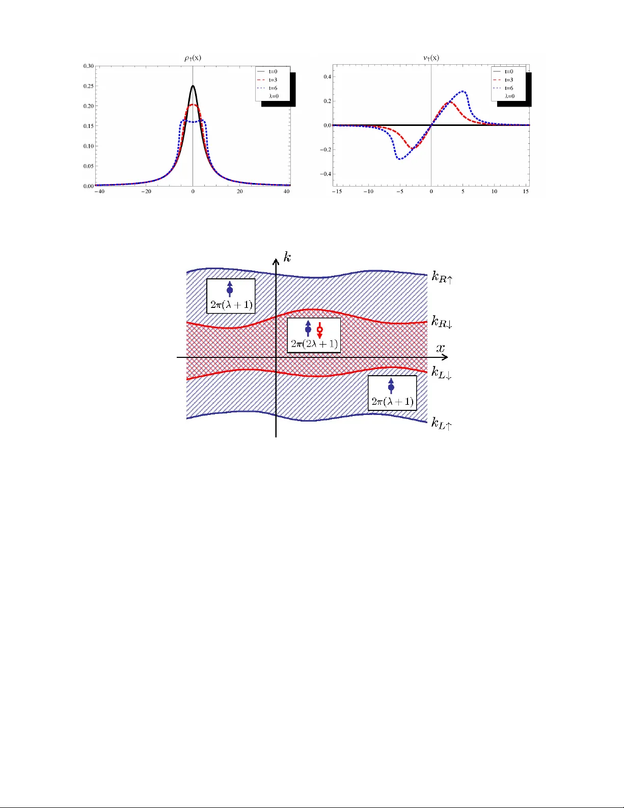
Nonlinear dynamics of spin and c harge in spin-Calogero mo del Manas Kulk arni 1 , 3 , F abio F ranchini 2 , Alexander G. Abanov 1 1 Dep artment of Physics and Astr onomy, Stony Bro ok University, Stony Br o ok, NY 11794-3800 2 The Ab dus Salam ICTP; Str ada Costier a 11, T rieste, 34100, Italy and 3 Dep artment of Condense d Matter Physics and Materials Scienc e, Br o okhaven National L ab or atory, Upton, NY-11973 The fully nonlinear dynamics of spin and c harge in spin-Calogero model is studied. The latter is an in tegrable one-dimensional model of quan tum spin-1/2 particles in teracting through inv erse-square in teraction and exchange. Classical h ydro dynamic equations of motion are written for this mo del in the regime where gradien t corrections to the exact hydrodynamic formulation of the theory may b e neglected. In this approximation v ariables separate in terms of dressed F ermi momenta of the mo del. Hydro dynamic equations reduce to a set of decoupled Riemann-Hopf (or inviscid Burgers’) equations for the dressed F ermi momenta. W e study the dynamics of some non-equilibrium spin- c harge configurations for times smaller than the time-scale of the gradient catastrophe. W e find an in teresting interpla y b etw een spin and charge degrees of freedom. In the limit of large coupling constan t the hydrodynamics reduces to the spin h ydro dynamics of the Haldane-Shastry model. Con tents I. In tro duction 2 I I. F ree fermions with spin 3 I I I. The spin-Calogero mo del 5 IV. Gradien tless hydrodynamics of spin-Calogero mo del 5 1. Spinless limit 7 2. λ = 0 – free fermions with spin 8 3. λ → ∞ limit. 8 V. Equations of motion and separation of v ariables 8 A. Equations of motion 8 B. F ree fermions ( λ = 0) and Riemann-Hopf equation 8 C. Riemann-Hopf Equations for sCM 9 VI. F reezing trick and h ydro dynamics of Haldane-Shastry mo del 10 A. O ( µ ) 11 B. O (1) 11 C. O (1 /µ ) 12 D. Ev olution equations for Haldane-Shastry mo del from the freezing trick 12 VI I. Illustrations 12 A. Charge dynamics in a spin-singlet sector 12 B. Dynamics of a p olarized center 13 1. Applicabilit y of gradientless hydrodynamics 13 2. F ree fermions with spin: λ = 0 13 3. λ -dep endence of spin and charge dynamics 13 VI I I. Conclusions 14 IX. Ac kno wledgments 15 A. Asymptotic Bethe Ansatz solution of spin Calogero Mo del and separation of v ariables in h ydro dynamics 15 B. Hydro dynamic v elo cities 17 2 C. Hydro dynamic regimes for spin-Calogero mo del 18 1. Conserv ed densities and dressed F ermi momenta 18 2. Complete Overlap Regime (CO) 20 3. P artial Overlap Regime (PO) 20 4. No Overlap Regime (NO) 21 5. All cases combined 22 D. Hydro dynamic description of Haldane-Shastry mo del from its Bethe Ansatz solution 23 References 24 I. INTR ODUCTION One-dimensional mo dels of many b o dy systems hav e b een a sub ject of intensiv e research since the seven ties. Due to the lo w dimensionality , standard p erturbativ e approaches dev elop ed in man y b o dy theory are often inapplicable. On the other hand some tec hniques specific to one spacial dimension are av ailable and allow to treat systems of in teracting particles non-p erturbativ ely . The F ermi Liquid paradigm is replaced b y the Luttinger Liquid theory 1 in one dimension. One of its most striking predictions is that at lo w energies spin and charge degrees of freedom decouple. One can say that at low energies physical electrons exist as separate spin and charge excitations. A t higher energies it is expected that spin and charge recombine in to the original electrons. One can see the traces of spin-charge in teraction taking into account corrections to the Luttinger liquid mo del arising from the finite curv ature of band disp ersion at F ermi energy 1 . The coupling betw een spin and charge in one-dimensional systems was studied b oth p erturbativ ely and using integrable mo dels av ailable in one dimension 2 . In this pap er we study the in teraction b etw een spin and charge in another integrable mo del – the spin-Calogero mo del (sCM). This mo del is a spin generalization 3,4,5 of the well-kno wn Calogero-Sutherland mo del 6 . Calogero-Sutherland type mo dels o ccupy a sp ecial place in 1D quantum physics. They are exactly solv able (inte- grable) but are very sp ecial even in the family of integrable mo dels. In particular, they can b e interpreted as systems of “non-interacting” particles with fractional exclusion statistics 6,7,8,9,10,11 . The sCM mo del is given by the following Hamiltonian: H ≡ − ~ 2 2 N X j =1 ∂ 2 ∂ x 2 j + ~ 2 2 X j 6 = l λ ( λ ± P j l ) ( x j − x l ) 2 (1) where we to ok the mass of particles as a unit y and P j l is the op erator that exchanges the p ositions of particles j and l 3 . The ± sign in the exchange term corresp onds to ferromagnetic and anti-ferromagnetic ground state resp ectiv ely if w e are studying fermions. Similarly , it corresp onds to an ti-ferromagnetic and ferromagnetic ground state resp ectively if we are considering b osonic particles. The four cases can b e summarized as: Bosons − →  + ⇒ An ti-ferromagnetic , − ⇒ F erromagnetic , F ermions − →  + ⇒ F erromagnetic , − ⇒ An ti-ferromagnetic . The coupling parameter λ is p ositiv e and N is the total num b er of particles. As it has b een already noted ab o ve the sCM is a very sp ecial mo del. In particular, in contrast to more generic in tegrable or non-integrable models the spin and charge in sCM are not truly separated even at lo w energies 4 . Of course, one can still describ e the low-energy excitation spectrum of sCM b y tw o indep endent harmonic fluid Hamiltonians, one for the charge and the other for spin. How ev er, it turns out that for the sCM the spin and charge v elo cities are the same 4 , i.e. spin and c harge do not actually separate. Here w e study the spin-Calogero mo del in the limit of an infinite num b er of particles using the hydrodynamic approac h. Alb eit, the collective field theory/quantum hydrodynamics of the spinless Calogero-Sutherland mo del has b een studied in great detail 12,13,14,15,16 , a complete understanding of its spin generalization is still lacking although a considerable progress has b een done recently in Refs. 17,18 . W e study the nonlinear collective dynamics of sCM in the semiclassical approximation, additionally neglecting gradien t corrections to the equations of motion. This limit is justified as long as we consider configurations with small gradien ts of density and velocity fields. The gradientless approximation is commonly employ ed in studying nonlinear equations 19 and allows to study the evolution for a finite time while the first nonlinear contributions are dominan t. 3 F or longer times, the solution will inevitably evolv e tow ard configurations with large field gradients (such as sho ck w av es) and the gradientless approximation b ecomes inapplicable. Nev ertheless, in the initial stage of the evolution, corrections due to gradient terms in the equations of motion can b e neglected (see further discussion in the Sec. V B). W e derive the gradientless hydrodynamics Hamiltonian from the Bethe Ansatz solution of the mo del. The paper is organized as follo ws. In Sec. I I w e start with the simplest spinful in tegrable model – a system of free fermions with spin. W e briefly review the Bethe Ansatz solution for spin-Calogero mo del in Sec. II I and deduce the hydrodynamic Hamiltonian for the sCM from this solution in Sec. IV neglecting gradient corrections. The corresp onding classical equations of motion are given in Sec. V. It is sho wn that v ariables separate and the system of h ydro dynamic equations is decoupled into four indep endent Riemann-Hopf equations for a giv en special linear com binations of density and velocity fields – the dressed F ermi momenta. In Sec. VI we illustrate that in the limit of strong coupling the hydrodynamics of sCM is reduced to the hydrodynamics of Haldane-Shastry lattice spin mo del giving the h ydro dynamic form ulation of the so-called fr e ezing trick 20 . W e present some particular solutions of the h ydro dynamic equations demonstrating nonlinear coupling b etw een spin and charge degrees of freedom in the sCM in Sec. VII and conclude in Sec. VI I I. T o av oid in terruptions in the main part of the pap er some imp ortant technical details are mov ed to the app endices and are organized as follows. In App endix A we use asymptotic Bethe ansatz to deriv e the hydrodynamics of sCM and to explain why v ariables separate in this system. In Appendix B w e describ e the notion of true hydrodynamic velocities. In App endix C we relate the h ydro dynamics of sCM to tw o infinite families of mutually commuting conserv ed quan tities and collect our results for the h ydro dynamics in the differen t regimes of sCM. Finally , in App endix D w e derive a hydrodynamic description of the Haldane-Shastry mo del from its Bethe Ansatz solution. I I. FREE FERMIONS WITH SPIN F or one-dimensional free fermions without internal degrees of freedom the low est state with a given total num ber of particles and total momen tum corresp onds to all single-particle plane wa v e states filled if the corresp onding momentum k satisfies k L < k < k R . Here k L,R are le ft and right F ermi momen ta resp ectiv ely which are defined by the given n umber of particles and momen tum of the system: N /L = Z k R k L d k 2 π = k R − k L 2 π = ρ , (2) P /L = Z k R k L d k 2 π ~ k = ~ k 2 R − k 2 L 4 π = ρv . (3) Here we introduced the (ov erall) velocity of the system v which is given from (2,3) by v / ~ = k R + k L 2 . (4) In verting (2,4) we express the left and right F ermi p oin ts k L,R in terms of the density ρ and velocity v as k R,L = v / ~ ± π ρ. (5) The energy of this state is given by E /L = Z k R k L d k 2 π ~ 2 k 2 2 = ~ 2 k 3 R − k 3 L 12 π = ρv 2 2 + ~ 2 π 2 6 ρ 3 . (6) Up to this moment ρ, v , k R,L are just n umbers c haracterizing the c hosen state of free fermions (only tw o of them are indep endent). Assuming the lo calit y of the theory we promote these num bers to quan tum fields and write the h ydro dynamic Hamiltonian of free spinless fermions as H = Z d x  ρ ( x ) v 2 ( x ) 2 + ~ 2 π 2 6 ρ 3 ( x )  = Z d x ~ 2 [ k R ( x )] 3 − [ k L ( x )] 3 12 π . (7) Here we consider ρ ( x ) and v ( x ) as quantum field op erators of density and velocity (and k R,L as given by (5)) having canonical commutation relations 21 [ ρ ( x ) , v ( y )] = − i ~ δ 0 ( x − y ) . (8) 4 Of course, gradient corrections to (7) are generically present and the ab o ve “deriv ation” is just a heuristic argument (semiclassical in nature). It turns out that (7) is, in fact, exact for free fermions. 44 It can b e derived rigorously either using the metho d of collective field theory 22,23,24 or conv en tional b osonization technique (but without linearization at F ermi p oints) 1,25,37 . The tw o terms of (7) hav e a very clear physical in terpretation. The first term is the kinetic energy of a fluid moving as a whole – the only v elocity term allo w ed by Galilean inv ariance. The second one is the kinetic energy of the in ternal motion of particles. This term is finite due to the Pauli exclusion principle. Within the hydrodynamic approach w e ha ve to think of this term as of an in ternal energy of the fluid. Comm uting the Hamiltonian (7) with the density and v elo cit y op erators one obtains the contin uit y and the Euler equations of quan tum h ydro dynamics. Alternativ ely , using [ k L ( x ) , k L ( y )] = − [ k R ( x ) , k R ( y )] = 2 π iδ 0 ( x − y ) the equations of motion can also b e written as a system of quantum Riemann-Hopf equations ˙ k R,L + ~ k R,L ∂ x k R,L = 0 . (9) F or free fermions with spin, w e simply add the Hamiltonians (7) written for spin up and spin down fermions: H = Z d x  1 2 ρ ↑ v 2 ↑ + 1 2 ρ ↓ v 2 ↓ + π 2 ~ 2 6  ρ 3 ↑ + ρ 3 ↓   . (10) Expanding (10) around the background density ρ 0 = k F π and the background velocity v 0 = 0 up to quadratic terms in v α and δ ρ α = ρ α − ρ 0 , we obtain the harmonic fluid approximation H ≈ ρ 0 2 Z d x  v 2 ↑ + π 2 ~ 2 δ ρ 2 ↑ + v 2 ↓ + π 2 ~ 2 δ ρ 2 ↓  ≈ ρ 0 4 ~ 2 X α = ↑ , ↓ Z d x  ( ∂ x φ R,α ) 2 + ( ∂ x φ L,α ) 2  (11) with righ t and left b osonic fields defined as ∂ x φ R ( L ) ,α = v α / ~ ± π δ ρ α . This pro cedure is equiv alen t to the con v entional linear b osonization pro cedure where the fermionic sp ectrum is linearized at the F ermi p oints. In the spin-charge basis, ρ c,s ≡ ρ ↑ ± ρ ↓ and v c,s = v ↑ ± v ↓ 2 , (12) the harmonic theory (11) is describ ed by a sum of tw o indep endent harmonic fluid Hamiltonians, one for charge and the other for spin degrees of freedom H ≈ ρ 0 4 Z d x  4 v 2 c + π 2 ~ 2 δ ρ 2 c + 4 v 2 s + π 2 ~ 2 δ ρ 2 s  . (13) After linearization, the quantum Riemann-Hopf Eq. (9) reduces to (where ± stands for χ = { R, L } resp ectively) ˙ k α,χ ± ~ π ρ 0 ∂ x k α,χ = 0 , α = {↑ , ↓} ; (14) from which we identify that the quadratic excitations propagate like wa v e equations with sound velocities u charg e = u spin = π ~ ρ 0 , equal for spin and charge. T urning on interactions b etw een fermions generally renormalizes spin and c harge sound v elocities differently and results in gen uine spin-charge separation at the lev el of harmonic approximation. The spin-Calogero-Sutherland mo del happ ens to b e very sp ecial in this resp ect. Despite a non-trivial interaction for spin and charge, their sound v elo cities remain the same. Although spin and charge are not truly separated for a free fermion system (and for the sCM), the in teraction b et w een spin and charge is absen t at the level of harmonic appro ximation (13). This interaction app ears if nonlinear corrections to (13) are tak en into accoun t (e.g., b y the fully nonlinear Hamiltonian (10)) and due to gradient corrections to the hydrodynamics. The latter are not considered in this pap er. In the prop er classical limit ~ → 0 all terms of (10) but the velocity terms v anish (F ermi statistics do es not exist for classical particles). Instead, we are in terested in a “semi-classical” limit in which ρ ∼ v / ~ . In this limit w e rescale time and velocity by ~ ( t → t/ ~ and v → ~ v ) and measure ev erything in length units. This is equiv alen t to dropping all ~ from equations. F or instance, the Hamiltonian (10) b ecomes H = Z d x  1 2 ρ ↑ v 2 ↑ + 1 2 ρ ↓ v 2 ↓ + π 2 6  ρ 3 ↑ + ρ 3 ↓   . (15) 5 W e replace the commutation relations (8) by the corresp onding classical Poisson brack ets (for up and do wn sp ecies) { ρ α ( x ) , v β ( y ) } = δ αβ δ 0 ( x − y ) (16) and consider the classical equations of motion generated by the Hamiltonian together with the Poisson brack ets. In the remainder of the pap er all h ydro dynamic equations are obtained in this semi-classic al limit. I II. THE SPIN-CALOGER O MODEL In this w ork w e concentrate on the hydrodynamics of sCM (1) for the case of spin-1 / 2 fermions with an anti- ferromagnetic sign of in teraction. It is conv enien t to imp ose perio dic boundary conditions, i.e. consider particles living on a ring of the length L . This Hamiltonian is given by H = − ~ 2 2 N X j =1 ∂ 2 ∂ x 2 j + ~ 2 2  π L  2 X j 6 = l λ ( λ − P j l ) sin 2 π L ( x j − x l ) (17) and is known to b e integrable 6 . All eigenstates of (17) can b e enumerated by the distribution function ν ( κ ) = ν ↑ ( κ ) + ν ↓ ( κ ) . (18) Here, κ are integer-v alued quantum n um b ers iden tifying a given state in a Bethe Ansatz description and ν ↑ , ↓ ( κ ) = 0 , 1 dep ending on whether a given κ is present in the solution of the Bethe Ansatz equations. The total momentum P and energy E of the eigenstate are giv en in terms of the distribution function ν ( κ ) as 26,27 : P =  2 π L  + ∞ X κ = −∞ κ ν ( κ ) , (19) E = E 0 +  1 2   2 π L  2 , (20)  = + ∞ X κ = −∞ κ 2 ν ( κ ) + λ 2 X κ,κ 0 | κ − κ 0 | ν ( κ ) ν ( κ 0 ) , (21) where E 0 = π 2 λ 2 6 N ( N 2 − 1) is the energy of a reference state 27 . The num bers of particles with spin up and spin do wn are separately conserved in (17) and are given by N ↑ , ↓ = + ∞ X κ = −∞ ν ↑ , ↓ ( κ ) . (22) The ground state wa v e function for (17) is 4,27 ψ GS = Y j 0. The opp osite case ρ s < 0 can b e obtained exchanging up and down v ariables. The other regimes and formulae v alid for all regimes are considered in detail in App endix C. In the CO regime (35), the Hamiltonian can b e written as H CO = Z d x ( 1 2 ρ ↑ v 2 ↑ + 1 2 ρ ↓ v 2 ↓ + λ 2 ρ ↓  v ↑ − v ↓  2 + π 2 λ 2 6 ρ 3 c + π 2 6  ρ 3 ↑ + ρ 3 ↓  + λπ 2 6  2 ρ 3 ↑ + 3 ρ 2 ↑ ρ ↓ + 3 ρ 3 ↓  ) . (36) 7 (a) – C omplete O verlap (b) – P artial O verlap (c) – N o O verlap FIG. 1: Distribution functions are shown for the three nonequiv alent regimes: Complete Overlap in (a), Partial Overlap in (b) and No Overlap in (c). Three additional regimes exist, but are physically equiv alent to the ones considered in these pictures and can b e obtained by exchanging ↑ ↔ ↓ . FIG. 2: Diagram capturing all cases It is obtained b y expressing (20,21) in terms of h ydrodynamic v ariables (29,30) using (35). As in the case of free fermions (see Sec. I I) we now consider ρ ↑ , ↓ ( x, t ) and v ↑ , ↓ ( x, t ) as space and time dep endent classical hydrodynamic fields with Poisson brack ets (16). Of course, going from the energy of the uniform state (25,26) to the nonuniform h ydro dynamic state we neglected gradients of densit y and velocity fields. W e refer to this approximation as to gr adientless hydr o dynamics . The equations of motion ge nerated by the Hamiltonian (36) with P oisson brack ets (16) can b e used only when gradients can b e neglected compared to the gradien tless terms. This means that one can use this gradientless hydrodynamics only at relatively small times (compared to the time of the gradient catastrophe, see the discussion b elow). Before analyzing more general case let us consider some sp ecial limits of (36). 1. Spinless limit In the fully polarized state ρ ↓ = 0 w e obtain from (36) the gradien tless Hamiltonian for spinless Calogero-Sutherland mo del H spinless = Z + ∞ −∞ dx  1 2 ρv 2 + π 2 6 ( λ + 1) 2 ρ 3  , (37) where w e dropped the subscript ↑ . The hydrodynamics (37) w as used in 29 to calculate the leading term of an asymptotics of a particular correlation function (Emptiness F ormation Probability) for the Calogero-Sutherland mo del. It can b e, of course, obtained by dropping gradient terms in the exact h ydro dynamics deriv ed using collective field theory 13,14,15 . 8 2. λ = 0 – fr e e fermions with spin A t the particular v alue λ = 0 the sCM reduces to free fermions with spin and the Hamiltonian (36) b ecomes the collectiv e Hamiltonian for free fermions (15). 3. λ → ∞ limit. In the limit of large coupling constant λ → ∞ the particles form a rigid lattice and charge degrees of freedom essen tially get frozen 20 . W e expect to arriv e to an effective spin dynamics equiv alent to the Haldane-Shastry model 30,31 (see App endix D). This reduction to the Haldane-Shastry mo del is usually referred to as fr e ezing trick 20 . W e analyze this reduction in more detail in Sec. VI. V. EQUA TIONS OF MOTION AND SEP ARA TION OF V ARIABLES A. Equations of motion The classical gradientless hydrodynamics for sCM is given by the Hamiltonian (36) with canonic P oisson’s brack ets (16). The classical evolution equations generated by this Hamiltonian are ˙ ρ ↑ = − ∂ x { ρ ↑ v ↑ + λρ ↓ ( v ↑ − v ↓ ) } , ˙ ρ ↓ = − ∂ x { ρ ↓ v ↓ − λρ ↓ ( v ↑ − v ↓ ) } , ˙ v ↑ = − ∂ x ( v 2 ↑ 2 + π 2 λ 2 2 ( ρ ↑ + ρ ↓ ) 2 + λπ 2  ρ 2 ↑ + ρ ↑ ρ ↓  + π 2 2 ρ 2 ↑ ) , (38) ˙ v ↓ = − ∂ x ( v 2 ↓ 2 + λ 2 ( v ↑ − v ↓ ) 2 + π 2 λ 2 2 ( ρ ↑ + ρ ↓ ) 2 + λπ 2 2  ρ 2 ↑ + 3 ρ 2 ↓  + π 2 2 ρ 2 ↓ ) . This is the system of con tinuit y and Euler’s equations for tw o coupled fluids (with spin up and spin down). W e can also rewrite it in terms of spin and charge v ariables (12) ˙ ρ c = − ∂ x { ρ c v c + ρ s v s } , ˙ ρ s = − ∂ x { ρ s ( v c − 2 λv s ) + (2 λ + 1) ρ c v s } , ˙ v c = − ∂ x  v 2 c 2 + (2 λ + 1) v 2 s 2 + π 2 8  (2 λ + 1) 2 ρ 2 c + (2 λ + 1) ρ 2 s   , (39) ˙ v s = − ∂ x  v c v s − λv 2 s + π 2 4 ρ s [(2 λ + 1) ρ c − λρ s ]  . One can see that spin and charge are not decoupled. It turns out, ho wev er, that the v ariables nevertheless separate and the system of four coupled equations (38) can b e written as four decoupled Riemann-Hopf equations (similar to (9)) for a sp ecial linear combinations of density and v elo cit y fields. In the following w e study the interaction of spin and charge gov erned by the ab o ve equations. B. F ree fermions ( λ = 0 ) and Riemann-Hopf equation A t λ = 0 equations (38) b ecome the hydrodynamic equations for free fermions. Fluids corresp onding to up and do wn spin are completely decoupled ˙ ρ ↑ , ↓ = − ∂ x { ρ ↑ , ↓ v ↑ , ↓ } , (40) ˙ v ↑ , ↓ = − ∂ x  1 2 v 2 ↑ , ↓ + π 2 2 ρ 2 ↑ , ↓  . (41) Let us introduce the following linear combinations of densities and v elo cities k R ↑ ,L ↑ = v ↑ ± π ρ ↑ , k R ↓ ,L ↓ = v ↓ ± π ρ ↓ . (42) 9 These com binations are nothing else but righ t and left F ermi momenta of free fermions. All of them satisfy the so-called Riemann-Hopf equation u t + uu x = 0 . (43) The equation is the same for all four combinations u = k R,L ; ↑ , ↓ and the system (40,41) is equiv alen t to four decoupled Riemann-Hopf equations. The Riemann-Hopf equation (43) is easily solv able with the general solution given implicitly by u = u 0 ( x − ut ) . (44) Here u 0 ( x ) is an initial profile of u ( x, t ) at t = 0. One should solv e (44) with respect to u and find u ( x, t ) - the solution of (43) with u ( x, t = 0) = u 0 ( x ). The solution (44) can also b e written in a parametric form x = y + t u 0 ( y ) , u ( x, t ) = u 0 ( y ) . (45) This solution corresp onds to the “Lagrangian picture” of fluid dynamics and states that p oints in the x − u plane are just translated along x with velocity u , i.e., ( x, u 0 ) → ( x + t u 0 , u 0 ). This picture is esp ecially useful to solve (43) n umerically . W e notice here that the nonlinear dynamics (43) without disp ersiv e (higher gradient) terms is ill defined at large times. F or any initial profile u 0 ( x ), at large times t > t c infinite gradients u x will develop - gr adient c atastr ophe - and solutions of (44) will b ecome multi-v alued. The classical equation (43) will not ha ve a meaning for t > t c . W e refer to the time t c (function of the initial profile) as to the gradient catastrophe time. The gradien tless hydrodynamics is applicable only for times smaller that t c . 46 W e will discuss in more detail about v alidit y of gradien tless h ydro dynamics in Sec. VI I. W e present a simple illustration of the density and velocity dynamics for free fermion system in Fig. 3. It is enough to consider only up-spin as the evolution of up and down spins is decoupled. W e chose the initial profile of the density as Lorentzian with the half-width a and height h ρ 0 ↑ ( x ) = h 1 + ( x/a ) 2 (46) and an initial v elocity zero. W e find the initial profiles of k ↑ ; R,L using (42). Then w e solve the Riemann-Hopf equations (43) using (45) and find the density and velocity at any time inv erting (42). W e remark that for an arbitrary smo oth bump of height h and width a the gradient catastrophe time can b e estimated as t c ≈ a h . F or the evolution giv en by (43) with an initial Lorentzian profile ( u 0 ( x ) given by (46)) one can compute the gradient catastrophe time exactly . An infinite gradient ∂ x u → ∞ develops at the time t c = 8 3 √ 3 a h . (47) F or arbitrary initial conditions we compute the gradient catastrophe time n umerically . C. Riemann-Hopf Equations for sCM Although the system of equations (38) is a system of four coupled nonlinear equations, it allows for a separation of v ariables. Introducing the linear com binations of fields k R ↑ ,L ↑ = v ↑ ± π [( λ + 1) ρ ↑ + λρ ↓ ] = ( v ↑ ± π ρ ↑ ) ± λπ ρ c , (48) k R ↓ ,L ↓ = ( λ + 1) v ↓ − λv ↑ ± π (2 λ + 1) ρ ↓ = ( v ↓ ± π ρ ↓ ) + λ ( − 2 v s ± 2 π ρ ↓ ) (49) w e obtain the Riemann-Hopf equation (43) separately for all four u = k L,R, ↑ , ↓ . This prop ert y of v ariable separation is shared with the free fermion case Sec.V B. W e notice, how ev er, that in the case of sCM, v ariables separate only in gradientless approximation. The gradien t terms neglected in this pap er will couple the hydrodynamic equations in an essential non-separable 47 w ay . The separation of v ariables in terms of (48,49) is not so surprising. One can recognize (48,49) as dressed (physical) “F ermi” momenta of (asymptotic) Bethe Ansatz. The integrals of motion of sCM are separated in terms of these 10 FIG. 3: Dynamics of density field ρ ↑ ( x ) (left panel) and of velocity field v ↑ ( x ) (right panel) for free a fermion case ( λ = 0). The initial densit y profile at t = 0 is a Lorentzian (46) of height h = 0 . 25 and half-width a = 4. The initial velocity is zero. FIG. 4: Phase-space diagram of a hydrodynamic state characterized by four space-dep endent F ermi momenta. F ermi momenta and the same is true for the equations of motion. W e do not interrupt the presentation with this connection with the Bethe Ansatz solution of sCM but devote the App endix A to this purp ose. It is conv enien t to summarize the gradien tless hydrodynamics of sCM by the picture in a “single-particle” phase space showing space-dep enden t F ermi momenta. 48 W e plot the space-dep endent F ermi momenta in an x − k plane as four smo oth lines. In the CO regime considered here (see App endix C for other regimes) the F ermi momenta are ordered as k L ↑ ( x ) < k L ↓ ( x ) < k R ↓ ( x ) < k R ↑ ( x ) . (50) W e fill the space b etw een those lines with particles ob eying the follo wing rules of particles with fractional exclusion statistics 11 (see App endix A) (i) each particle o ccupies a phase space v olume 2 π ( λ + 1) if there are no particles of the other sp ecies in this volume, (ii) tw o particles with opp osite spins o ccupy a phase space v olume 2 π (2 λ + 1) (or 2 π ( λ + 1 / 2) p er particle). The v elo cit y v ↑ ( x ) is visualized as a center of a spin-up strip e on Figure 4 (see (B5)). The in terpretation of v ↓ ( x ) is a bit less straightforw ard. It should b e thought as a weigh ted av erage of p ositions of centers of b oth strip es (B5). VI. FREEZING TRICK AND HYDROD YNAMICS OF HALDANE-SHASTR Y MODEL Here we consider the limit of large coupling constant λ → ∞ . In this limit we exp ect that particles form a one- dimensional lattice and only spin dynamics is imp ortan t at low energies. W e refer to this limit as to a freezing of the 11 c harge. W e are in terested in fluctuations around the uniform state with a given charge density . It can b e seen from Fig. 4 that particles o ccupy the volume 2 π ( λ + 1 / 2) of the phase space when b oth sp ecies are presen t. Therefore, the natural expansion parameter is µ = λ + 1 / 2 instead of λ . 49 W e will see that the leading in µ term of the dynamics results in c harge freezing, while the next to leading term giv es the non-trivial spin dynamics of the lattice model kno wn as the Haldane-Shastry mo del 30,31 H HSM = 2 X j 0, i.e., for the ordering k L ↑ < k L ↓ < k R ↓ < k R ↑ , (C10) are k R ↑ ,L ↑ = v ↑ ± π [( λ + 1) ρ ↑ + λρ ↓ ] = v ↑ ± π ρ ↑ ± λπ ρ c , k R ↓ ,L ↓ = ( λ + 1) v ↓ − λv ↑ ± π (2 λ + 1) ρ ↓ = v ↓ ± π ρ ↓ + λ ( − 2 v s ± 2 π ρ ↓ ) . (C11) P oisson’s brack ets of k α are giv en by (C3) with coefficients from the T able I. One can express all conserved densities (C1) in terms of dressed F ermi momenta using the T able I. F or example, the Hamiltonian (see (C2)) reads H CO = 1 12 π ( λ + 1) Z d x  k 3 R ↑ − k 3 L ↑ + 1 2 λ + 1  k 3 R ↓ − k 3 L ↓   (C12) = Z d x ( 1 2 ρ ↑ v 2 ↑ + 1 2 ρ ↓ v 2 ↓ + λ 2 ρ ↓  v ↑ − v ↓  2 + π 2 λ 2 6 ρ 3 c + π 2 6  ρ 3 ↑ + ρ 3 ↓  + λπ 2 6  2 ρ 3 ↑ + 3 ρ 2 ↑ ρ ↓ + 3 ρ 3 ↓  ) . (C13) The evolution equations are given b y (C4) and can also b e recast in terms of equations for densities and velocities (38,39). 3. P artial Overlap Regime (PO) There are tw o regimes when the supp orts of ν ↑ and ν ↓ only partially ov erlap. Here we concentrate on the case for whic h π 2 | ρ s | < v s < π 2 ρ c , (C14) corresp onding to the ordering k L ↓ < k L ↑ < k R ↓ < k R ↑ . (C15) The other PO regime can b e obtained b y exchanging up and down particles, i.e. by changing v s → − v s . In this case the dressed momenta (A2) are k L ↓ = v ↓ − π ( λ + 1) ρ ↓ − π λρ ↑ = v ↓ − π ρ ↓ − λπ ρ c , k L ↑ = v ↑ + λ ( v ↑ − v ↓ ) − π (2 λ + 1) ρ ↑ = v ↑ − π ρ ↑ + λ (2 v s − 2 π ρ ↑ ) , k R ↓ = v ↓ − λ ( v ↑ − v ↓ ) + π (2 λ + 1) ρ ↓ = v ↓ + π ρ ↓ − λ (2 v s − 2 π ρ ↓ ) , k R ↑ = v ↑ + π ( λ + 1) ρ ↑ + π λρ ↓ = v ↑ + π ρ ↑ + λπ ρ c (C16) 21 FIG. 7: Phase-space diagrams of a hydrodynamic states characterized by four space-dependent F ermi momen ta in three regimes CO, PO, and NO resp ectiv ely . and the Hamiltonian b ecomes (see T able I and (C1,C2)) H PO = 1 12 π ( λ + 1) Z d x  k 3 R ↓ − k 3 L ↑ + 1 2 λ + 1  k 3 R ↑ − k 3 L ↓   (C17) = Z d x ( 1 2 ρ ↑ v 2 ↑ + 1 2 ρ ↓ v 2 ↓ + λπ ρ ↑ ρ ↓ ( v ↓ − v ↑ ) − λ 12 π [ v ↑ − v ↓ − π ( ρ ↑ + ρ ↓ )] 3 + π 2 λ 2 6 ( ρ ↑ + ρ ↓ ) 3 + π 2 6 (1 + 2 λ )  ρ 3 ↑ + ρ 3 ↓  ) . (C18) P oisson’s brack ets of k α are given by (C3) with co efficien ts from the T able I and evolution equations are given by (C4). 4. No Overlap Regime (NO) In this case, the supp orts of ν ↑ and ν ↓ do not ov erlap at all. F or v s > 0 the ordering of dressed F ermi momen ta is k L ↓ < k R ↓ < k L ↑ < k R ↑ (C19) and momenta themselves are k R ↑ ,L ↑ = v ↑ + π λρ ↓ ± π ( λ + 1) ρ ↑ = v ↑ ± π ρ ↑ ± λπ ρ c,s , k R ↓ ,L ↓ = v ↓ − π λρ ↑ ± π ( λ + 1) ρ ↓ = v ↓ ± π ρ ↓ − λπ ρ s,c . (C20) and the Hamiltonian b ecomes (see T able I and (C1,C2)) H NO = 1 12 π ( λ + 1) Z d x  k 3 R ↑ − k 3 L ↑ + k 3 R ↓ − k 3 L ↓  (C21) = Z d x ( 1 2 ρ ↑ v 2 ↑ + 1 2 ρ ↓ v 2 ↓ + λπ ρ ↑ ρ ↓ ( v ↑ − v ↓ ) + π 2 6 ( λ + 1) 2 ( ρ ↑ + ρ ↓ ) 3 − π 2 2 (1 + 2 λ ) ρ ↑ ρ ↓ ( ρ ↑ + ρ ↓ ) ) . (C22) P oisson’s brack ets of k α are given by (C3) with co efficien ts from the T able I and evolution equations are given by (C4). 22 k inequality v s ρ s ξ 1 = v s + π 2 ρ s ξ 2 = v s − π 2 ρ s χ 1 = v s + π 2 ρ c χ 2 = v s − π 2 ρ c v s inequalit y Regime k L ↑ < k R ↑ < k L ↓ < k R ↓ − − − − − v s < − π 2 ρ c NO k L ↑ < k L ↓ < k R ↑ < k R ↓ − − − + − − π 2 ρ c < v s < − π 2 | ρ s | PO k L ↓ < k L ↑ < k R ↑ < k R ↓ − − + + − π 2 ρ s < v s < − π 2 ρ s CO k L ↑ < k L ↓ < k R ↓ < k R ↑ + + − + − − π 2 ρ s < v s < π 2 ρ s CO k L ↓ < k L ↑ < k R ↓ < k R ↑ + + + + − π 2 | ρ s | < v s < π 2 ρ c PO k L ↓ < k R ↓ < k L ↑ < k R ↑ + + + + + π 2 ρ c < v s NO T ABLE I I: Classification of different regimes: + indicates that the field takes p ositiv e v alues, − that it is negative. A blank means that its sign is arbitrary . 5. All cases combined It is p ossible to combine all hydrodynamic regimes in to relatively compact expressions in tro ducing absolute v alues of hydrodynamic fields. A general Hamiltonian v alid for all regimes takes a form H = Z d x ( 1 2 ρ ↑ v 2 ↑ + 1 2 ρ ↓ v 2 ↓ + π 2 6  ρ 3 ↑ + ρ 3 ↓  + π 2 6 λ 2 ρ 3 c + π 2 3 2 λ ( ρ 3 ↑ + ρ 3 ↓ ) + λ ρ c ξ 1 ξ 2 − λ 3 π  | ξ 1 | 3 + | ξ 2 | 3  + λ 3 π  | χ 1 | 3 − χ 3 1 + | χ 2 | 3 + χ 3 2  ) , (C23) where we introduced the following notations ξ 1 , 2 ≡ v s ± π 2 ρ s , (C24) χ 1 , 2 ≡ v s ± π 2 ρ c . (C25) The Hamiltonian (C23) can b e obtained from (20,21) for the general case of a tw o-step distribution function ν ↑ , ↓ ( κ ). W e collect in the T able I I the information necessary to go quickly from the general expression (C23) to the particular ones v alid in separate regimes (CO, PO or NO). W e can combine the evolution equations following from (C23) in the spin/charge basis (12) as ˙ ρ c = − ∂ x n ρ c v c + ρ s v s o , (C26) ˙ ρ s = − ∂ x ( ρ c v s + ρ s v c − λ π h ξ 1 | ξ 1 | + ξ 2 | ξ 2 | − χ 1 | χ 1 | − χ 2 | χ 2 | i ) , (C27) ˙ v c = − ∂ x ( v 2 c + v 2 s 2 + π 2 8 h  4 λ 2 + 2 λ + 1  ρ 2 c + (2 λ + 1) ρ 2 s i + λ 2 h χ 1 | χ 1 | − χ 2 | χ 2 | i ) , (C28) ˙ v s = − ∂ x ( v c v s + π 2 4 (2 λ + 1) ρ c ρ s − λ 2 h ξ 1 | ξ 1 | − ξ 2 | ξ 2 | i ) . (C29) F or CO and PO regimes the Hamiltonian (C23) takes an esp ecially simple form in terms of dressed momenta H CO & PO = 1 12 π (2 λ + 1) Z d x ( k 3 R ↑ − k 3 L ↑ + k 3 R ↓ − k 3 L ↓ + λ ( λ + 1) h   k 3 L ↑ − k 3 L ↓   +   k 3 R ↑ − k 3 R ↓   i ) , (C30) whic h are related to densit y and velocity fields as k R ↑ ,L ↑ = v ↑ ± π ( λ + 1) ρ ↑ + λχ 1 , 2 ∓ λ | ξ 1 , 2 | , k R ↓ ,L ↓ = v ↓ ± π (1 + λ ) ρ ↓ − λχ 2 , 1 ∓ λ | ξ 1 , 2 | . (C31) As in the separate cases considered b efore, these momenta hav e canonical Poisson’s brack ets (A17) with s R ↑ ,R ↓ = ( λ + 1) [ λ + 1 ± λ sgn ( ξ 1 )] s L ↑ ,L ↓ = − ( λ + 1) [ λ + 1 ∓ λ sgn ( ξ 2 )] (C32) and evolv e indep enden tly according to the Riemann-Hopf equations (C4). 23 APPENDIX D: HYDROD YNAMIC DESCRIPTION OF HALDANE-SHASTR Y MODEL FROM ITS BETHE ANSA TZ SOLUTION The Haldane-Shastry mo del (HSM) is a Heisenberg spin c hain with long-ranged interaction defined by the Hamil- tonian: H HSM = 1 2 X j t c . It is the b oundary of the supp ort of the Wigner distribution in the one-particle phase space. In this pap er we restrict ourselv es to times less than the time of gradient catastrophe and assume that (43) has a well-defined single-v alued solution. 47 A t least one will not b e able to separate v ariables considering simple linear combinations of fields. T o the best of our kno wledge v ariables in sCM do not separate or, at least, an appropriate c hange of v ariables has not b een found y et. 48 W e would like to thank A. Polyc hronak os who encouraged us to present this picture. 49 Of course, first orders of the expansion are not sensitive to this shift. 50 In exotic cases inv olving b oundaries b etw een CO and PO regimes one notices singularities dev eloping at the boundary and w e expect gradient corrections to correct these singularities. 51 Note that for fermions P j l K j l = − 1. 52 This corresp onds to ha ving a single compact supp ort of ν within a single Brillouin zone. Other regimes will require an analysis of umklapp pro cesses 41 and will not b e considered here. 53 This scattering phase is iden tical to the one in λ = 2 b osonic Calogero-Sutherland mo del 30 .