Finite Word Length Effects on Transmission Rate in Zero Forcing Linear Precoding for Multichannel DSL
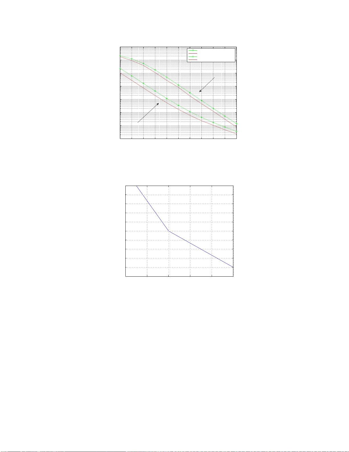
Crosstalk interference is the limiting factor in transmission over copper lines. Crosstalk cancelation techniques show great potential for enabling the next leap in DSL transmission rates. An important issue when implementing crosstalk cancelation te…
Authors: Eitan Sayag, Amir Leshem, Nikolaos D. Sidiropoulos
1 Finite W ord Length Ef fects on T r ansmission Rate in Zero F o rcing Linea r Precoding for Multichannel DSL Eitan Sayag 1 , 2 , Amir Leshem 1 , 3 Senior member , IEEE and Nicholas D. Sidiropoulos 4 Senior member , IEEE Abstract Crosstalk interferen ce is the limitin g facto r in transmission over copper lines. Crosstalk cancelatio n technique s show great p otential for ena bling the n ext leap in DSL tra nsmission rates. An impor tant issue when implementin g crosstalk cancelatio n techniq ues in hardware is the effect of finite world len gth on perfor mance. In this paper we p rovide an analysis of the perfo rmance of linear zero-for cing p recoders, used for crosstalk comp ensation, in the presence of finite word length errors. W e quantif y analytically the trade off between preco der word length and tr ansmission rate degradation . More specifically , we prove a simple formu la f or the transmission rate loss as a functio n of th e nu mber of bits used for preco ding, the signal to noise ratio, and the standar d line parameters. W e dem onstrate, thro ugh simulations on real lines, the accuracy of our estima tes. Mo reover , our results are stable in the presence of ch annel estimation error s. Finally , we show how to u se the se estimates a s a design to ol for DSL linear cro sstalk precod ers. For example, we sh ow that for standar d VDSL2 precoded systems, 14 bits re presentation o f the pr ecoder entries results in capacity loss below 1 % for line s over 300m . Keywords: Multich annel DSL, vectoring, linear preco ding, c apacity estimates, q uantization. 1 School of Engineering, Bar-Ilan Univ ersity , 52900, Ramat Gan, I srael. 2 Dept. of Math. Ben Gurion Univ ersity , Beer-Shev a, Israel. 3 Circuit an d Systmes, Faculty of EEMCS, Delft Uni versity of T echnolog y , Delft, The Netherlands. 4 Dept. of EC E, T echnical Univ ersity of Crete, Greece. This research was partially supported by the E U-FP6 IST , und er contract no. 506790, and by the Israeli ministry of trade and commerce as part of Nehusha \ iSMAR T project. Conference version of part of this work appeared in Proc. IEE E I CASSP 2008 , Mar . 30 - Apr . 4, 2008, L as V egas, Nev ada. June 5, 2021 DRAFT 2 I . I N T R O D U C T I O N DSL systems are capable of delive ring high data rates over copper lines. A major problem of DSL technologies is t he electromagnetic coupling between the t wisted pairs within a binder group. Reference [1] and the recent experimental studies in [2], [3] have demonstrated that vectoring and cr osstalk can celation all ow a s ignificant increase o f t he data rates of DSL systems. In particular , lin ear precoding has recently drawn consi derable attention [4], [5] as a natural method for crosstalk precompensation as well as cross talk ca ncelation in the recei ver . In [2], [3] it is shown that op timal cancelation achie ves capacity boost ranging from 2 × to 4 × , and also substantiall y reduces per -loop capacity spread and outage, which are very important m etrics from an operator’ s perspecti ve. R eferences [5], [6] advocate the use of a diagonalizing precompensator , and demonstrate that, without m odification of the Customer Pre mise Equipm ent (CPE), one can obtain near optimal performance. Recent work in [7], [8] has shown that a low- order t runcated series approxim ation of t he i n verse channel m atrix aff ords significant complexity reduction i n the computation of the precodin g matrix. Implementation com plexity (i.e., the actual mul tiplication of the transm itted symbol vector by th e precodin g matrix) remains high, howe ver , especially for m ulticarrier transm ission which requires one matri x-vector multipli cation for each tone. Current advanced DSL systems use thousands of tones. In t hese conditio ns, using m inimal word length in representing t he precoder matrix i s im portant. Howe ver , usi ng coarse quanti zation will resul t in substantial rate loss. The num ber of quantization bit s per matrix coefficient is an important parameter that affects the system’ s performance - compl exity trade-off, which we focus on in this p aper . W e provide closed form sharp anal ytic bou nds on the abso lute and relativ e transmiss ion rate loss. W e show that both absolute and relativ e transmiss ion loss decay exponentially as a function of the number o f quantizer bits and provide explicit bo unds for the loss in each t one. Under analytic channel mo dels as in [9], [10] we provide refi ned and explicit bounds for the transm ission loss across the band and com pare these to simulat ion results . This explicit relationsh ip between the number of quantizer bits and the transmissi on rate loss due to quantization is a ver y useful tool in th e desig n of practical sys tems. The structure of the p aper is as follows. In section II, we present the signal mod el for a precoded discrete m ultichannel sy stem and provide a model for the precoder errors we study . In s ection III, a general formula for t he t ransmission loss of a singl e user is derive d. In section June 5, 2021 DRAFT 3 IV we focus on the case o f full channel st ate info rmation where the rate loss of a si ngle u ser results from quantization errors only . Here we prove the main result of the paper , Theorem 4.1. W e provide e xplicit bounds on the rate loss under an analytic model for the transfer function as in [9]. W e also study a number of natural design criteria. In section V we provide sim ulation results on measured l ines, which support our analy sis. Moreover , we show through sim ulation that our result s are valid in the presence of measurement errors. Th e appendices provide full details of the m athematical claims u sed in the main t ext. I I . P RO B L E M F O R M U L A T I O N A. Sign al model In t his section we describe th e sig nal model for a precoded discrete m ultitone (DMT) system. W e assu me that the transmission scheme i s Frequency Division Duplexing (FDD), where the upstream and the downstream t ransmissions are performed at separate frequency bands. M ore- over , we assu me that all modems are synchronized. Hence, the echo sign al i s eliminated, as in [1], and the received sign al model at frequency f is given by x ( f ) = H ( f ) s ( f ) + n ( f ) , (1) where s ( f ) is th e vectored s ignal sent by the optical network unit (ONU), H ( f ) is a p × p matrix representing the channels , n ( f ) is additive Gaussian noi se, and x ( f ) (conceptually) coll ects the signals received by t he individual us ers. The us ers estim ate rows of th e channel m atrix H ( f ) , and the ONU uses this information to send P ( f ) s ( f ) instead of s ( f ) . This process is called cr ossta lk pr e-compensation . In general such a m echanism yields x ( f ) = H ( f ) P ( f ) s ( f ) + n ( f ) . (2) Denote the diagonal o f H ( f ) b y D ( f ) = diag ( H ( f )) and let P ( f ) = H ( f ) − 1 D ( f ) as s uggested in [5]. W ith this we ha ve x ( f ) = D ( f ) s ( f ) + n ( f ) , (3) showing that the crosstalk is elim inated. Not e that wit h F ( f ) = H ( f ) − D ( f ) we hav e th e following formula for the matrix P ( f ) P ( f ) = I + D − 1 ( f ) F ( f ) − 1 . (4) June 5, 2021 DRAFT 4 Follo wing [5] we ass ume that the matrices H ( f ) are ro w-wise diagonall y dominant, namely that k h ii k >> k h ij k , ∀ i 6 = j. (5) In fact, mo tiv ated in part by Gersgorin’ s theorem [11] we propose the parameter r ( H ) r ( H ) = max 1 ≤ i ≤ N P j 6 = i | h ij | | h ii | , (6) as a measure for the dominance. In most downstream scenarios the parameter r is indeed much smaller than 1. W e emphasize that typical downstream VDSL channels are ro w-wi se diagonally dominant e ven in mixed leng th scenarios as demons trated i n [8]. B. A model for pr ecoder err ors In practical implement ations, the entries of the precoding matri x P will be quant ized. The number o f q uantizer bits used is dict ated by complexity and memory considerations. Indeed, relativ ely coarse quanti zation of the entries of the precoder P allows significant reduction of the time complexity and the amount of memory needed for the precodin g process. The key p roblem is to determine the transmission rate loss of an individual user caused by such quantizatio n. Another clo sely related problem is the issue of robustness of linear precoding with respect t o errors in the estimation of the channel matrix. The mathematical setting for both is th at of error analysis. Let P = ( I + D − 1 F + E 1 ) − 1 + E 2 , (7) where • E 1 models the r elati ve err or in quan tizing or measur ing the channel matri x H , and • E 2 models the err ors caus ed by quantizing the precoder P . The prob lem is t o determine the capacity of t he system , and th e capacity of each us er , in terms of the system p arameters and the st atistical p arameters of t he errors. Not e that equ ation (7) captures three types o f errors: errors in th e estimation of H , quantization errors in the representation of H , and quantization errors in the representation of the precoder P . Our focus will be in the stu dy of the ef fect of quantization errors in the representation of the precoder on the capacity of an indi vidual user . Nev ertheless, the estimation errors result ing from measuring t he channel cannot be ignored. W e will show that the analysis of quantization errors and estimation errors can b e dealt separately (see remark 3.2 after lemma 3.1). This allows June 5, 2021 DRAFT 5 us to carry analys is under th e assumption o f perfect channel in formation. Then, we show in simulatio ns that when the estimatio n errors in channel measurement s are reasonably sm all, our analytical bounds remain valid. C. System Model W e now list our assumpt ions regarding the errors E 1 , E 2 , the power spectral density of the users, and the beha v ior of t he channel m atrices. Pe rfect CSI: Perfect Channel Information. Namely , E 1 ( f ) = 0 , ∀ f . (8) Quant (2 − d ) : The quantization error of each matrix element of t he precoder is at most 2 − d . Namely , | E 2 ( f ) i,j | ≤ 2 − d , ∀ f , ∀ i, j. (9) DD: The channel m atrices are row-wise d iagonally dominant. r ( H ( f )) ≤ 1 , ∀ f . (10) SPSD: The Po w er Spectral Density (PS D) o f all the users of the binder is the same. Namely , we assume that for some fixed unspecified function P ( f ) we ha ve: P i ( f ) = P ( f ) , ∀ i. (11) The m ain result of the paper , Theorem 4.1 i s based o n assumptions (8), (9), (10), (11). Assumptio n SPSD can be li fted, as s hown in section XIV (appendi x H ). For the sake of clarity we present only the sim plified result i n t he body of t he paper . In order t o o btain sharp analytic estimat es on the transmi ssion loss in actual DSL scenarios we need to incorporate s ome of the properties of the channel m atrices of DSL channels in to our model. In particular , we will assume W ern er Channel model: The matrix elem ents o f the channel m atrices H ( f ) behave as in the model of [9]. Namely , following [9] we assume the follo wing m odel for i nsertion l oss | H I L ( f , ℓ ) | 2 = e − 2 αℓ √ f (12) June 5, 2021 DRAFT 6 where ℓ is the DSL loop length (in meters), f is th e frequency i n Hz, and α is a parameter that depends on the cable type. Furthermore, crosstalk i s m odeled as | H F E X T ( f , ℓ ) | 2 = K ( ℓ ) f 2 | H I L ( f , ℓ ) | 2 (13) Here K ( ℓ ) is a random variable studied in [10]. The findi ng is that K ( ℓ ) is a log-norm al distribution with expectation, deno te t here c 1 ( ℓ ) , that increase linearly wit h ℓ . An additional assumption that we will m ake concerns the behavior of th e ro w dominance of the channel matrices H ( f , ℓ ) . Sub li near row dominance: r ( H ( f , ℓ )) ≤ γ 1 ( ℓ ) + γ 2 ( ℓ ) f (14) Where γ 2 ( ℓ ) = O ( √ ℓ ) . Remark 2.1: Note that | H F E X T ( ℓ, f ) | | H I L ( f , ℓ ) | = p K ( ℓ ) f . The sub-linearity in f follows by study ing r ( H ( ℓ, f )) in terms of p 2 random v ariables behaving as K ( ℓ ) . D. Justification of the assumptions Pe rfect CSI i s plausible due to the quasi -stationarity of DSL systems (long coherence tim e), which allo ws us to est imate the channel matrices at high precision. Quant (2 − d ) is a weak assumpt ion on the t ype of the quantization process. Informally it i s equiv alent to an assumption on the number of bits used to quantize an entry in the channel m atrix. In particular , our analysis of the capacity loss will be independent of the specific quant ization method and our re sults are v al id for any technique that quantizes mat rix elements wit h bounded errors. Assumptio n DD reflects the diagonal dom inance of DSL channels. While linear precoding may result in power fluctuations, the diagonal do minance property of DSL channel m atrices makes these fluctuations negligibl e within 3.5d B fluctuation allo wed by PSD templ ate (G993.2 ). For example if the row dominance is up to 0.1 th e eff ect of precoding on the transmi t powers and spectra will be at most 1dB. June 5, 2021 DRAFT 7 Assumptio n SPSD (see (11)) is just ified in a system with i deal full-binder precoding, where each user will use the entire PSD mask all owe d by regulation. Note that i n [3] it is shown that DSM3 provides signi ficant capacity gains only when almost all pairs i n a binder are coordi nated. Thus the equal t ransmit spectra assumption is reasonable in these systems . Howe ver we also provide in section XIV (appendix H) a generalization of t he main result to a sett ing in which this assumption is not sati sfied. Assumptio n W erner Channel model does not need justification whereas our last assum ption, sub-linear r ow dominance was ve rified on measured lines [3] and can also be deduced analyt- ically from W erner ’ s model. In practice, the type of fitting requi red to obt ain γ 1 ( ℓ ) , γ 2 ( ℓ ) from measured data is sim ple and can be done ef ficiently . Moreove r , the line parameters tabulated in standard (e.g., R,L,C,G p arameters of the two port mo del), t ogether w ith the 99% worst case power sum model used in standards [12], provide another way of com puting the constants γ 1 ( ℓ ) , γ 2 ( ℓ ) . I I I . A G E N E R A L F O R M U L A F O R T R A N S M I S S I O N L O S S The purpose of this section is to provide a general formula for t he transmis sion rate loss of a si ngle u ser , resulting from errors i n the estim ated channel matrix as well as errors in the precoder matrix . First, we de velop a useful expression for th e equiv al ent channel in t he presence of errors. This is given in form ula (17). Next, a form ula for the transmission loss is obtained (30). Th e formul a compares the achiev able rate of a comm unication system using an ideal ZF precoder as in (4) versus th at of a communication syst em whose precoder is giv en by (7). This formula is the key to the whole paper . Not e that we use a gap analysi s as in [13], [14]. A useful corollary in the form of formula (34) is derived. This wil l be used in the next s ection to obtain bounds on capacity loss du e to qu antization. Let H ( f ) = D ( f ) + F ( f ) be a decompositi on of th e channel matrix at a giv en frequency to diagonal and no n-diagonal terms. Thus D ( f ) is a diagonal matrix whose diagonal is ident ical to the diagonal of H ( f ) . Also we let S N R i ( f ) be th e sig nal to noise ratio of the i -th receiv er at frequency f S N R i ( f ) = P i ( f ) | d i,i ( f ) | 2 E | n i ( f ) | 2 . (15) In this formula P i ( f ) is the power spectral density (PSD) of the i -th user at frequency f , and June 5, 2021 DRAFT 8 n i ( f ) is the associated no ise t erm. W e denote σ 2 n i ( f ) = E | n i ( f ) | 2 . (16) A. A formula for the equivalent channel in the pr esence of err o rs W e first derive a g eneral formula for the equiv alent s ignal mod el. The next lemma provides a useful reformu lation of the signal model in (2): Lemma 3.1: The precoded channel (2) with precoder as in (7) is giv en by x ( f ) = D ( f ) s ( f ) + D ( f ) ∆ ( f ) s ( f ) + n ( f ) , (17) with ∆ ( f ) = ( I + D − 1 ( f ) F ( f )) E 2 ( f ) − E 1 ( f )( I + D − 1 ( f ) F ( f ) + E 1 ( f )) − 1 . (18) The proof i s deferred t o appendix A (section VII). Remark 3.2: For our analysis, we wi ll assume that E 1 ( f ) = 0 , in which case the formula for the matrix ∆ simplifies to ∆ ( f ) = ( I + D − 1 ( f ) F ( f )) E 2 ( f ) . (19) The relev ance of the formula (18) for the experimental part of the paper (where E 1 ( f ) is not assumed to be zero) i s explained in the next remark. Remark 3.3: In formula (30) b elow w e show that t he impact of th e errors E 1 ( f ) and E 2 ( f ) on the transmission loss of a user can be computed from the m atrix ∆ . Thus, an important consequence of the lemm a is that the ef fect on transm ission loss due to estimation er rors (encoded in the matri x E 1 ( f ) ) and due t o quantization errors (encoded in the mat rix E 2 ( f ) ) can be stud ied separately as they contribute to different terms in the above expression for ∆ . B. T ransmissio n Loss of a Sin gle Us er Consider a comm unication system as defined i n (3) and denote by B the frequency band of the system . W e let S N R i ( f ) be as in (15) and let Γ be t he Shannon Gap comprising modulatio n loss, coding gain and nois e mar gin. Let R i be the achiev able transmission rate of the i -th user in the s ystem defined in (3). Recall that in such a syst em the crosstalk is completely removed and therefore R i = Z f ∈ B log 2 (1 + Γ − 1 S N R i ( f )) d f . (20) June 5, 2021 DRAFT 9 Let R i ( f ) = lo g 2 (1 + Γ − 1 S N R i ( f )) (21) be th e transmissi on rate at frequency f (formally , it is j ust the density of that rate). Let ˜ R i ( f ) be the transmi ssion rate at frequenc y f of the i -th user , when the p recoder i n (7) is used. W e note that whi le R i ( f ) is a number , t he quantity ˜ R i ( f ) depends on th e random variables E 1 , E 2 and hence is itself a random variable. Let ˜ R i be the transmissio n rate of the i -th user for th e equiv alent system in (17). Thus, ˜ R i = Z f ∈ B ˜ R i ( f ) d f . (22) By equation (17), the i -th user receiv es x i ( f ) = d i,i ( f ) s i ( f ) + d i,i p X j =1 ∆ i,j ( f ) s j ( f ) + n i ( f ) = d i,i ( f )(1 + ∆ i,i ( f )) s i ( f ) + N i ( f ) (23) where N i ( f ) = d i,i ( f ) P p j 6 = i ∆ i,j ( f ) s j ( f ) + n i ( f ) . Assu ming Gaussian s ignaling i.e. that all s i ( f ) are Gaussian we conclude that N i ( f ) is Gaussian. A simil ar conclusion is v alid in the case of a lar ge number of users, due to the Central Limit Theorem. In p ractice, the Gaussi an assumpti on is a good approximation even for a modest number of (e.g., 8) users. Recall also that Gaussian signaling is the optimal strategy in the case of exact channel k nowledge. Therefore, we can use the capacity form ula for the Gauss ian channel, e ven under precoder q uantization errors. Definition 3.1: The transmission loss L i ( f ) of the i -th us er at frequenc y f is given by L i ( f ) = R i ( f ) − ˜ R i ( f ) . (24) The total l oss of the i -th user is L i = Z f ∈ B L i ( f ) d f . (25 ) W e are ready to deduce a fo rmula for t he rate loss of the i - th user as a result of the no n-ideal precoder in (17). Our result will be gi ven in terms of the matrix ∆ . Recall that ∆ generally depends on both precoder quant ization errors E 2 and estimation errors E 1 . Denote by ∆ i,j the ( i, j ) -th element of the matrix ∆ and let δ i ( f ) = Γ X j 6 = i P j ( f ) P i ( f ) | ∆ i,j ( f ) | 2 . (26) Let June 5, 2021 DRAFT 10 a i ( f ) = δ i ( f )Γ − 1 S N R i ( f ) = X j 6 = i P j ( f ) P i ( f ) | ∆ i,j ( f ) | 2 S N R i ( f ) , (27) q i ( ∆ , f ) = | 1 + ∆ i,i ( f ) | 2 a i ( f ) + 1 , (28) and k i ( f ) = Γ − 1 S N R i ( f ) Γ − 1 S N R i ( f ) + 1 . (29 ) Note that a i ( f ) and hence q i ( ∆ , f ) are independent of the Shannon gap Γ . The next lemma provides a formula for the exact t ransmission rate loss d ue to t he errors modeled by the m atrices E 1 and E 2 . The result i s stated i n terms of qu antities q ( ∆ , f ) and the effecti ve signal to noise ratio, Γ − 1 S N R i ( f ) . Lemma 3.4: Let H ( f ) be the channel matrix at frequency f and let E 1 , E 2 be t he esti mation and quantization errors, respecti vely as in (7). Let L i ( f ) be t he loss in transm ission rate o f the i -th user defined in (24). Then L i ( ∆ , f ) = − log 2 (1 − k i ( f )(1 − q i ( ∆ , f ))) , (30) where q i ( ∆ , f ) is g iv en in (28) and k i ( f ) is gi ven in (29). In particular , if ∆ i,i ( f ) = − 1 the transmis sion loss i s log 2 (1 + Γ − 1 S N R i ( f )) , where S N R i ( f ) is defined i n (15). Finally , if ∆ i,i ( f ) 6 = − 1 we have L i ( ∆ , f ) ≤ M ax 0 , log 2 1 q i ( ∆ , f ) (31) The p roof of this lemma i s d eferred to app endix B (section V III). T o formulate a useful corollary we introdu ce the quanti ties: M i ( f ) = max j 6 = i P j ( f ) P i ( f ) (32) t i ( f ) = max 1 ≤ j ≤ n | ∆ i,j | (33) Cor ollar y 3.5: L et H ( f ) be the p × p channel matrix at frequency f and let E 1 ( f ) , E 2 ( f ) be the estimation and qu antization errors respectively as in (7). Let L i ( f ) be t he transm ission rate loss of the i -th user defined in (24). Assume that t i ( f ) < 1 . Then L i ( ∆ , f ) ≤ log 2 1 + ( p − 1) M i ( f ) t 2 i ( f ) S N R i ( f ) (1 − t i ( f )) 2 (34) June 5, 2021 DRAFT 11 Pr oof : By (27) we ha ve a i ( f ) = X j 6 = i P j ( f ) P i ( f ) | ∆ i,j ( f ) | 2 S N R i ( f ) ≤ M i ( f ) t i ( f ) 2 ( p − 1) S N R i ( f ) (35) 1 + a i ( f ) ≤ 1 + ( p − 1) M i ( f ) t i ( f ) 2 S N R i ( f ) (36) Since | ∆ i,i ( f ) | ≤ t i ( f ) we get | 1 + ∆ i,i ( f ) | 2 ≥ (1 − t i ( f )) 2 (37) Thus by (28) we have 1 q i ( ∆ , f ) = a i ( f ) + 1 | 1 + ∆ i,i ( f ) | 2 ≤ 1 + ( p − 1) M i ( f ) t 2 i ( f ) S N R i ( f ) (1 − t i ( f )) 2 (38) Notice that the right hand si de is l ar ger than one and using (31) of the pre vio us lemma the proo f is complete. Remark 3.6: W e note that under sim plifying assumptions, such as assumption SPSD (see (11)) the above formula reduces to L i ( ∆ , f ) ≤ log 2 (1 + ( p − 1) t 2 i ( f ) S N R i ( f )) − 2 lo g 2 (1 − t i ( f )) (39) Under t he assum ption Perfect CSI , we hav e ∆ ( f ) = ( I + D − 1 ( f ) F ( f )) E 2 ( f ) and si nce we further assu med that the channel m atrices H ( f ) are row-wise diagonally dom inant we s ee that ∆ ( f ) ≈ E 2 ( f ) . Thus, t i ( f ) ≈ 2 − d and we obtain a b ound of the form L i ( ∆ , f ) ≤ log 2 (1 + ( p − 1) S N R i ( f )2 − 2 d ) − 2 log 2 (1 − 2 − d ) (40) For a statement of a bound of t his form see formula (41) of Theorem 4.1 below . I V . T R A N S M I S S I O N R A T E L O S S R E S U LT I N G F R O M Q UA N T I Z A T I O N E R R O R S I N T H E P R E C O D E R In t he ZF precoder st udied earlier we can assum e wit hout lo ss o f generality that the entries are of absolute value less than one. Each of these v alues is now represented using 2 d bits ( d bits for the real part and d bit s for the imaginary part, not includi ng the sign bit). W e first consider an ideal s ituation in which we have perfect channel estimatio n. June 5, 2021 DRAFT 12 A. T ransmissio n Loss with P erfect Channel Knowledge Consider the case where E 1 = 0 and the quantization error is gi ven by an ar bitrary matrix E 2 with th e property that each entry is a com plex n umber w ith real and imagin ary parts bounded in absolute v alue by 2 − d . W e will not make an y further assum ptions about the particular quantization method employed and we will provide up per bounds for t he capacity lo ss. W e do not assume any specific random mod el for the values of E 2 because we are interested in obt aining absolute upper bounds o n capacity loss. The following theorem describes the transm ission rate loss resulting from quantization of the precoder . Main Theorem 4.1: Let H ( f ) be the channel matri x of p twis ted pairs at frequency f , and r ( f ) = r ( H ( f )) as in (6). Assume Perfect CSI (8), Q uant (2 − d ) (9), SPSD (11), and that the precoder P ( f ) is q uantized usin g d ≥ 1 2 + log 2 (1 + r ( f )) bits. Th e transm ission rate l oss of the i -th user at frequency f d ue to q uantization i s bounded by L i ( d, f ) ≤ log 2 (1 + γ ( d, f ) S N R i ( f )) − 2 lo g 2 (1 − v ( f )2 − d ) , (41) where γ ( d, f ) = 2( p − 1)(1 + r ( f )) 2 2 − 2 d (42) and v ( f ) = √ 2(1 + r ( f )) . (43) Furthermore, suppose d ≥ 1 2 + log 2 (1 + r max ) with r max = max f ∈ B ( r ( H ( f )) . (44) Then the transmission loss in the band B is at most Z f ∈ B log 2 (1 + γ ( d ) S N R i ( f )) d f − 2 | B | log 2 (1 − ( 1 + r max )2 − d +0 . 5 ) , (45) where | B | is the tot al b andwidth, γ ( d ) = 2 (1 + r max ) 2 ( p − 1)2 − 2 d , (46) The p roof of the theorem i s d eferred to s ection IX (appendi x C). W e now record some useful corollaries of t he th eorem illustrating it s v alue. June 5, 2021 DRAFT 13 Cor ollar y 4.2: T he t ransmission rate l oss L i ( ∆ , f ) , due to quantization of the precodin g matrix by d bits is bounded by : L i ( ∆ , f ) ≤ log 2 (1 + γ ( d, f ) S N R i ( f )) − 2 lo g 2 (1 − v ( f )2 − d ) (47 ) where γ ( d, f ) = 2( p − 1) ( 1 + r ( f )) 2 2 − 2 d and v ( f ) = √ 2(1 + r ( f )) . If r ( f ) ≤ 1 , a s implified looser bound is gi ven by L i ( ∆ , f ) ≤ 2 − d +3 . 5 + log 2 (1 + 8( p − 1) S N R i ( f )2 − 2 d ) (48) For the deriv ati on of the first inequali ty see (91) in section IX. The simplified bound i s based on the estimate − log 2 (1 − z ) ≤ 2 z valid for 0 ≤ z ≤ 0 . 5 . The n ext result is of theoretical v alue. It describes th e asym ptotic behavior of L i ( d ) for very lar ge d . Cor ollar y 4.3: U nder th e assumptions of the theorem and assuming that r max ≤ 1 : L i ( d ) = O (2 − d ) . More precisely , we have L i ( d ) = θ √ 32 ln(2) 2 − d B ! . Remark 4.4: By definition, f ( n ) = θ ( g ( n )) i f and only i f lim n →∞ f ( n ) g ( n ) = 1 W e note that for many practical values of the parameters (e.g. S N R ( f ) = 80 dB , d ≤ 20 , p ≤ 100 ) t he first term in form ula (45 ), in volving 2 − 2 d , is dominant. Since we are i nterested i n results that have relev ance to existing systems we will de velop in the next secti on, and under some further assumptions (e.g. ass umptions (12), (13)), a boun d for L i ( d ) of the form a 1 2 − 2 d + a 2 2 − d where t he coefficients a 1 , a 2 are expressible using the system parameters. This i s propo sition 4.8. Ensuring bounded transmission loss in each freq uency bin W e now turn to study the natural design requirement that the transm ission loss caused due to quantization of precoders should be bounded by a certain fixed qu antity , say 0.1b it/sec/Herz/user , on a per -tone basis . Such a design criterion is examined in the next corollary . Cor ollar y 4.5: L et t > 0 and let d be an integer with d ≥ d ( t ) (49) June 5, 2021 DRAFT 14 W ith d ( t ) = log 2 (1 . 25 v ( f )2 t +1 /tl n (2 )) if 2 t − 1 ≤ B 2 4 A 0 . 5 log 2 (5( p − 1)(1 + r ) 2 S N R i ( f ) /tl n (2)) otherwise Then the transmission loss at tone f d ue to q uantization with d bi ts is at mo st t b ps/Hz. Pr oof : By theorem 4.1, the loss at a tone f is bounded by log 2 1 + 2 − 2 d u ( f )) − log 2 ((1 − v ( f )2 − d ) 2 ) . Where u ( f ) = 2( p − 1)(1 + r ) 2 S N R i ( f ) and v ( f ) = √ 2(1 + r ( f )) . Using 1 − 2 t ≤ (1 − t ) 2 we get L i ( d, f ) ≤ log 2 1 + 2 − 2 d u ( f )) − log 2 (1 − 2 v ( f )2 − d ) . W e will show that the inequality log 2 1 + 2 − 2 d u ( f ) 1 − 2 v ( f )2 − d ≤ t (50) is satisfied for any d ≥ d ( t ) as i n (49) Let z = 2 − d so that the in equality (50) is 1 + z 2 u ( f ) 1 − 2 v ( f ) z ≤ 2 t (51) This yields a quadratic inequality of the form Az 2 + B z ≤ T (52) with A = u ( f ) , B = 2 t +1 v ( f ) and T = 2 t − 1 . U sing lemm a 10.1 (see section X - app endix D), we see that if d ≥ d 0 ( t ) where d 0 ( t ) = log 2 (1 . 25 v ( f )2 t +1 / (2 t − 1) if 2 t − 1 ≤ B 2 4 A 0 . 5 log 2 (5( p − 1)(1 + r ) 2 S N R i ( f ) / (2 t − 1)) otherwise Then L i ( d, f ) ≤ t . But d 0 ( t ) ≤ d ( t ) because 2 t − 1 ≥ l n (2 ) t and the result follo ws. Remark 4.6: The qualitativ e behavior is d ( t ) ≈ a 1 − log 2 ( t ) for very small v alues of t whereas d ( t ) ≈ a 2 − 0 . 5 lo g 2 ( t ) for lar ger v alues o f t . B. Appl ications of the Main Theor em W e no w apply theorem 4.1 to analyze the required quant ization level for DSM level 3 precoders under se veral design criteria. T o th at end let R i be the t ransmission rate of the i -th user (20) and let L i be the transmis sion lo ss of t he i -th user as in (24). The r elative transmission los s is defined by June 5, 2021 DRAFT 15 η i = L i R i = Z f ∈ B L i ( f ) d f / Z f ∈ B R i ( f ) d f (53) The d esign criteria are • Absolute/relative transmission loss across the band is bounded. • Absolute/relative transmission loss for each tone is bounded. Bound on Absolute T ransmission Loss From now on, we will ass ume that the transfer function obeys a parametric model as in [9]. Thus we assume (12) and (13). T o bound the absolute transm ission loss we estimate the integral in formu la (45) of theorem 4.1. Using the m odel (12) one can easily see that S N R i ( f ) = P i ( f ) σ 2 n i ( f ) e − 2 αℓ √ f Moreover , under the assum ption (14) we h a ve a linear bou nd on the quantity r ( H ( f , ℓ )) that is, r ( H ( f , ℓ )) ≤ γ 1 ( ℓ ) + γ 2 ( ℓ ) f Where γ 2 )( ℓ ) = O ( √ ℓ ) . Putt ing t hese t ogether we can estimate the integral occurring in the bound (45) and the final conclusi on in described in theorem 4.8. The p arameters γ 1 ( ℓ ) , γ 2 ( ℓ ) enter our b ounds through the foll owing quantity . ρ ℓ = (1 + γ 1 ( ℓ )) 2 + 12(1 + γ 1 ( ℓ )) γ 2 ( ℓ ) ( αℓ ) 2 + 240 γ 2 ( ℓ ) ( αℓ ) 2 ) 2 (54) Remark 4.7: The quantity ρ ℓ beha ves as 1 + C ℓ − 3 / 2 and is close to one for ℓ = 300 m. W e are no w ready to form ulate o ne of the mai n resul ts of this p aper: Theor em 4.8: Under assumption s P erfect CSI , Quant (2 − d ) , SPSD , W erner model and s ub- linear row dominance (see (8), (9), (11), (12), (13 ), (14)) we h a ve L i ( d ) B ≤ ξ ℓ 2 − 2 d + 2 − d +3 . 5 (55) where ξ ℓ = 4 ln(2) ( p − 1) P σ 2 n 1 α 2 B 1 ℓ 2 ρ ℓ (56) W e provide a proof of this result in section XI(appendix E). June 5, 2021 DRAFT 16 Bound on Relative T ransmission Loss The m ost natural design criterion is to ensure that the re lative capacity loss i s b elow a pre- determined threshold. W e will keep our assumption that the insertion l oss beha ves as in the model (12), (13). Let S N R i = P i σ 2 n i and S N R ′ i = P i σ 2 n i e − α √ B be the Sign al to Noise ratios of t he i -th us er at the lowest and highest frequencies. W e also denote b y ] S N R = S N R i Γ and by ^ S N R ′ i = S N R ′ i Γ . Finally , we denote c i = 1 3 log 2 ( ^ S N R i ) + 2 3 log 2 ( ^ S N R ′ i ) (57) The next propositi on sho ws that c i provides a lowe r bound on the spectral efficienc y of the i -th user . Pr opos ition 4.1: Assu me that the attenuation transfer characteristic of the channel is give n b y (12). Then the spectral efficiency is bounded below by 1 B R i ≥ c i (58) The p roof is deferre d to section 4.1 (appendix F). Cor ollar y 4.9: L et η i ( d ) be t he relative transmi ssion rate loss of the i -th user as in (53). Assume that the transfer funct ion satisfies (12) and (13). Then η i ( d ) ≤ ζ ℓ 2 − 2 d + 1 c i 2 − d +3 . 5 (59) where ζ ℓ = ξ ℓ c i = 4 ln(2) ( p − 1) P σ 2 n 1 α 2 B 1 ℓ 2 1 c i ρ ℓ . (60) Pr oof : This is an im mediate consequence of the upper bound on t he average loss L i B and the lower bound on 1 B R i . Ensuring bounded relativ e transmission loss in the whole band The next corollary yields an upper bound for the number of quantized bits required to ensure that the relati ve loss is below a giv en threshold. Cor ollar y 4.10: Let 0 ≤ τ ≤ 1 and let d ≥ d ( τ ) where d ( τ ) = log 2 ( 12 √ 2 c i τ ) if τ ≤ 32 ζ ℓ c 2 0 . 5 log 2 ( 2 . 5 ζ ℓ τ ) otherwise Then the relati ve transmiss ion loss caused by quantization with d bits is at m ost τ . The proof is a simple appl ication of the previous bo und on th e relative t ransmission loss and lemma 10.1 (section X - appendix D). June 5, 2021 DRAFT 17 V . S I M U L A T I O N R E S U LT S T o check the quality o f t he bounds in theorem 4.1 and it s corollaries, we compared the bounds with s imulation results, based o n measured chann els. W e have used the results of the measurement campaign conducted by France T elecom R & D as described in [10]. All experiments used the band 0 − 30 MHz. Full band For each experiment, we generated 1000 random precoder qu antization error matrices E 2 ( f ) , with i.i.d. elements, and independent real and im aginary parts, each uniformly d istributed in the interval [ − 2 − d , 2 d ] . W e add the error matrix to the precoder matrix to generate the quantized precoder m atrix. Repeating thi s in each frequenc y we prod uced a sim ulation of the quantized precoded system and comput ed the resulting channel capacity of each of the 10 users. Then we computed the re lative and absolute capac ity loss of each of the users. In eac h bin we picked the worst case out of 1000 qu antization t rials and obtained a quantity we called maximal loss . The quantity maxim al loss is a random variable depending on the n umber o f bits used to quanti ze the precoder matrices. E ach v alue of this random variable provides a lowe r bound for the actual worst case that can occur when th e channel m atrices are quant ized. W e com pare this l owe r bound with ou r upp er bound s of theorem 4.1. W e have check ed our bou nds in the foll owing scenario: Each user has flat PSD o f -60dBm/Hz, the noise has flat PSD o f -14 0dBm/Hz. The Shannon Gap is assumed to be 10 . 7 dB . As can be seen in figure 1, the bound given by (45) is sharp. W e also check ed the mo re e xplicit bou nd (59 ) which is based on the model (12), (13). W e v alidated the l inear behavior of the row d ominance r ( H ( f )) as a function of the tone f as predicted by formula (14). Next we used (12) to fit the parameter α of the cable via the measured insertion losses. The process of fitting is described in d etail in [10]. Its v alue whi ch was us ed in t he bound (59) was α = 0 . 0019 . Th e parameters γ 1 = 0 . 1596 and γ 2 = 3 . 1729 10 − 8 were estimated from the measured channel matrices by sim ple lin e fit. The results are depicted in Figure 1. Single fr equency The bounds provided for the entire band are results of bound s on each frequenc y bin. T o show that our bounds ar e sharp e ven without a veraging ove r the frequency band, we st udied the capacity los s in specific frequenc y b ins. W e concentrated on the same scenario as before (i.e. June 5, 2021 DRAFT 18 with 10 users), the noise is − 140 dB m/H z and the power of th e users is − 60 dB m/H z . W e picked measured matrices H ( f 1 ) , H ( f 2 ) , so that S N R ( f 1 ) is 40 d B m and S N R ( f 2 ) is 60 d B m . As before, we s ystematically generated an error matrix E 2 by choosing its entri es to be i.i.d., uniformly distrib uted with maxim al absolut e value 2 − d +0 . 5 . Ne xt, we compu ted t he transm ission rate los s using formula (30). By repeating this process N = 100 00 tim es and choo sing the worst e vent of transmissi on rate loss, we obtained a lower boun d est imate of worst-case transmissio n rate los s. This was compared to the bounds o f corollary 4.2. The results are depicted in figure 2. Figure 2 uses formul a (47). In particular we see th at for S N R = 60 d B and trans mission rate l oss of one percent, simulati on indicates quantization with 13 bits. The analytic formula indicates 14 bits . Similarly , when S N R = 4 0 dB , and again allo wing the same transmissi on rate loss of one percent, simulation suggests using 10 bits for quant ization. The si mple analytic estimate requires 11 b its. The number of quantizer bit s needed t o as sur e 99 per cent of capacit y In t he next experiment we hav e studied the number of bits required to obtain a given trans- mission los s as a function of the loop length. Figure 3 depicts the number of bits required to ensure transmissi on rate lo ss below o ne percent as a function of loo p length. W e see that 14 bits are suf ficient for l oop lengths up to 1200m. Fewer bits are required for longer loops. Stability of t he r esults In t he next e xperiment w e validated that the analytic resu lts proven for perfect CSI are v alid e ven when CSI is i mperfect as long as channel measurement errors are not t he do minating cause for capacity loss . T o model the measurement errors o f the channel matrix H ( f ) , we us ed matrices wit h Gaussian entries wi th variance which is prop ortional to S N R ( f ) . More precisely we assumed that the es timation err or of t he matrix H ( f ) is a Gaussi an wit h zero mean and wit h var iance σ 2 H ( f ) = 1 N S N R i ( f ) , where N is the n umber of samples used to estimate the channel matrix H ( f ) . F or N = 100 0 , we estimated the loss in a frequency bin as the worst case out of 500 realizations of qu antization nois e comb ined with m easurement noise. Figure 3 shows that as long as th e quantization noi se is dominant we can safely use our boun ds for t he transmission loss. W e comment that the stationarity o f DSL channels allows accurate channel estim ation. June 5, 2021 DRAFT 19 V I . C O N C L U S I O N S In this paper we analyzed finite word length effe cts on the achiev able rate of vector DSL systems with zer o forcing precoding. The result s of this paper provide simple analyti c e xpressions for the loss due to finite word lengt h. T hese expressions allow simple optimizati on of linearly precoded DSM le vel 3 systems. W e v alidated our result s using m easured channels. Moreover , we s howed that our bounds can be adapted to study the ef fect o f measurement errors on the t ransmission loss . In practice for loop lengths between 300 and 1200 meters, one needs 1 4 bits to represent the precoder elements in order t o lose no more than on e percent o f the capacity . V I I . A P P E N D I X A : P R O O F O F L E M M A 3 . 1 In t his section w e prov e lem ma 3.1. Pr oof : For simplicit y we will omit the explicit dependency of the matrices H ( f ) , D ( f ) , F ( f ) , P ( f ) on the frequenc y f . W e sh ow that HP = D + D ∆ , (61) with ∆ as above. Indeed H = D ( I + D − 1 F ) and thus HP = D ( I + D − 1 F )(( I + D − 1 F + E 1 ) − 1 + E 2 ) . (62) Hence, HP = D ( I + D − 1 F + E 1 − E 1 )( I + D − 1 F + E 1 ) − 1 + D ( I + D − 1 F ) E 2 . (63) Thus, HP = D − DE 1 ( I + D − 1 F + E 1 ) − 1 + D ( I + D − 1 F ) E 2 , (64) Which prov es t he lemma. V I I I . A P P E N D I X B : P RO O F O F L E M M A 3 . 4 In t his appendix we prove l emma 3.4. Pr oof : By equation (17), the i -th user receive s x i ( f ) = d i,i ( f ) s i ( f ) + d i,i p X j =1 ∆ i,j ( f ) s j ( f ) + n i ( f ) = d i,i ( f )(1 + ∆ i,i ( f )) s i ( f ) + N i ( f ) (65) June 5, 2021 DRAFT 20 with N i ( f ) = d i,i ( f ) P p j 6 = i ∆ i,j ( f ) s j ( f ) + n i ( f ) . For a large number of us ers, we may assume that N i ( f ) is again a Gaussian n oise and the transmission rate at frequency f of the s ystem described by equation (65 ) will be R i (∆ , f ) = log 2 1 + P i ( f ) | d i,i ( f ) | 2 | (1 + ∆ i,i ( f )) | 2 Γ( P j 6 = i P j ( f ) | d i,i ( f ) | 2 | ∆ i,j ( f ) | 2 + | n i ( f ) | 2 ) ! (66) Note that this quantity app eared in the main body of th e paper j ust after equation (22) where it was d enoted ˜ R i ( f ) . Di viding both th e num erator and denom inator by P i ( f ) | d i,i ( f ) | 2 we get R i (∆ , f ) = log 2 1 + | (1 + ∆ i,i ( f )) | 2 Γ P j 6 = i P j ( f ) P i ( f ) | ∆ i,j ( f ) | 2 + Γ | n i ( f ) | 2 P i ( f ) | d i,i ( f ) | 2 (67) or R i (∆ , f ) = log 2 1 + | (1 + ∆ i,i ( f )) | 2 δ i ( f ) + 1 eS N R i ( f ) ! (68) where we ha ve defined eS N R i ( f ) = S N R i ( f ) Γ = P i ( f ) | d i,i ( f ) | 2 Γ | n i ( f ) | 2 (69) and δ i ( f ) = Γ X j 6 = i P j ( f ) P i ( f ) | ∆ i,j ( f ) | 2 (70) T o get the transmission rate loss we deno te eS N R i (∆ , f ) = | (1 + ∆ i,i ( f )) | 2 δ i ( f ) + 1 eS N R i ( f ) (71) Notice that eS N R i ( f ) = eS N R i ( 0 , f ) By definition (24) we have L i ( ∆ , f ) = R i ( f ) − R i (∆ , f ) = log 2 (1 + eS N R i ( f )) − lo g 2 (1 + eS N R i (∆ , f )) (72) W e then hav e L i ( ∆ , f ) = − log 2 1 + eS N R i (∆ , f ) 1 + eS N R i ( f ) = − log 2 1 − eS N R i ( f ) − eS N R i (∆ , f ) 1 + eS N R i ( f ) (73) But eS N R i ( f ) − eS N R i (∆ , f ) = eS N R i ( f ) − | (1 + ∆ i,i ( f )) | 2 δ i + 1 eS N R i ( f ) (74) June 5, 2021 DRAFT 21 so eS N R i ( f ) − eS N R i (∆ , f ) = eS N R i ( f ) δ i ( f ) + 1 − | (1 + ∆ i,i ( f )) | 2 δ i + 1 eS N R i ( f ) (75) and finally , eS N R i ( f ) − eS N R i (∆ , f ) = eS N R i ( f ) eS N R i ( f ) δ i ( f ) + 1 − | (1 + ∆ i,i ( f )) | 2 δ i ( f ) eS N R i ( f ) + 1 (76) Hence L i ( ∆ , f ) = − log 2 1 − eS N R i ( f ) eS N R i ( f ) + 1 a i ( f ) + 1 − | 1 + ∆ i,i | 2 a i ( f ) + 1 (77) where a i ( f ) = δ i ( f ) eS N R i ( f ) ( 78) and δ i ( f ) is gi ven in (70). W ith the notations (28) and (29) we get the formula L i ( ∆ , f ) = − log 2 (1 − k i ( f )(1 − q i ( ∆ , f ))) (79) T o prove the bound w e cons ider two cases. When q ( ∆ , f ) > 1 we see from equation (79) that L i ( ∆ , f ) ≤ 0 . This clearly indicates transmission gain and the stated inequ ality is v alid. On the other hand, if q i ( ∆ , f ) ≤ 1 we get eS N R i eS N R i + 1 (1 − q i ( ∆ , f )) ≤ 1 − q i ( ∆ , f ) (80) and using t he monotonicity of − log 2 (1 − u ) (increasing) in the int erv al ( 0 , 1 ) , we get L i ( ∆ , f ) ≤ − log 2 (1 − ( 1 − q i ( ∆ , f )))) = log 2 1 q i ( ∆ , f ) (81) and the Lemma is proved. I X . A P P E N D I X C : P R O O F O F T H E O R E M 4 . 1 For the proof of the theorem we need a si mple lem ma. Lemma 9.1: Let A be a complex p × p matrix and define D to be the diago nal matrix with D i,i = A i,i for i = 1 , .., p . Let E be a p × p matrix whose entries are complex num bers with real and imaginary parts bounded by 2 − d . Finally , let B = D − 1 AE . Then | B i,j | ≤ 2 − d +1 / 2 (1 + r ( A )) . Pr oof : Let Q = D − 1 A = I + D − 1 ( A − D ) . Then we ha ve p X k =1 | Q ik | ≤ 1 + r ( A ) (82) June 5, 2021 DRAFT 22 for all i = 1 , .., p . Therefore | B i,j | = p X k =1 Q ik E k j ≤ 2 − d +1 / 2 p X k =1 | Q ik | ≤ 2 − d +1 / 2 (1 + r ) (83) Pr oof of the main theorem W e first bound the l oss L i ( f ) in a p articular to ne f . By Lemma 3.4 we ha ve L i ( ∆ , f ) ≤ M ax 0 , log 2 1 q i ( ∆ , f ) (84) where q i ( ∆ , f ) = | 1 + ∆ i,i ( f ) | 2 a i ( f ) + 1 (85) Here ∆ ( f ) = ( I + D ( f ) − 1 F ( f )) E 2 ( f ) wh ere H ( f ) = D ( f ) + F ( f ) is the channel matrix at frequency f and E 2 ( f ) is a matrix whose entries are complex numbers with real and imagi nary parts bound ed by 2 − d . Applyi ng Lemma (9.1) to th e matrix H ( f ) we see t hat the entries ∆ i,j ( f ) are all in a dis k of radius v ( f )2 − d around zero. Using r ( f ) ≤ 5 we obtain v ( f ) = √ 2(1 + r ( f )) ≤ 6 √ 2 . Using d ≥ 4 we get 1 − 2 − d v ( f ) ≥ 1 − 6 √ 2 16 > 0 . Thus | 1 + ∆ i,i ( f ) | 2 ≥ (1 − v 2 − d ) 2 . (86) Using the ass umption on th e PSD of the different users we obtain a i ( f ) = X j 6 = i P j ( f ) P i ( f ) | ∆ i,j ( f ) | 2 S N R i ( f ) = X j 6 = i | ∆ i,j ( f ) | 2 S N R i ( f ) . (87) Using Lemma (9.1) we have X j 6 = i | ∆ i,j ( f ) | 2 ≤ ( p − 1)2 − 2 d +1 (1 + r ( f )) 2 , (88) thus, 1 + a i ( f ) ≤ 1 + ( p − 1)2 − 2 d +1 (1 + r ( f )) 2 S N R i ( f ) = 1 + γ ( d, f ) S N R i ( f ) . (89) Combining (85), (86) and (89) we obtain 1 q i ( ∆ , f ) ≤ 1 + γ ( d, f ) S N R i ( f ) (1 − v ( f )2 − d ) 2 (90) June 5, 2021 DRAFT 23 Note that the right hand sid e of the a bove inequality is positiv e and greater than one. Combining (31) and (90) we obtain L i ( ∆ , f ) ≤ log 2 1 + γ ( d, f ) S N R i ( f ) (1 − v ( f )2 − d ) 2 = log 2 (1 + γ ( d, f ) S N R i ( f )) − 2 lo g 2 (1 − v ( f )2 − d ) (91) Since γ ( d, f ) ≤ 2(1 + r max ) 2 ( p − 1)2 − 2 d and v ( f ) = √ 2(1 + r ( f )) ≤ √ 2(1 + r max ) , i ntegrating this inequality ov er f ∈ B we obtain (45) and the theorem i s p rove d. X . A P P E N D I X D : P R O O F S O F C O R O L L A RY 4 . 8 A N D 4 . 9 A. A Quadratic Inequal ity In t he proof of corollary 4.8 and corollary 4.9 we use the fol lowing lemma. Lemma 10.1: Let A, B , T b e positive real numbers and let d ( T ) = log 2 (1 . 25 B /T ) if T ≤ B 2 4 A 0 . 5 log 2 (2 . 5 A/T ) otherwise Then for d ≥ d ( T ) we ha ve A 2 − 2 d + B 2 − d ≤ T (92) Pr oof : W e let x = 2 − d and obs erve that f ( x ) = Ax 2 + B x is monotone in x > 0 with on e root of f ( x ) = T exactly at x 0 = √ B 2 +4 AT − B 2 A . T hus for any d > d 0 ( T ) = log 2 ( 2 A √ B 2 +4 AT − B ) we hav e A 2 − 2 d + B 2 − d = f (2 − d ) ≤ f (2 − d 0 ) = f ( x 0 ) = T . T o complete the proo f w e wi ll show that d 0 ( T ) ≤ d ( T ) . Indeed, d 0 ( T ) = log 2 2 A √ B 2 + 4 AT − B = log 2 2 A ( √ B 2 + 4 AT + B ) 4 AT ! (93) Thus, d 0 ( T ) = log 2 B 2 T ( r 1 + 4 AT B + 1) ! (94) If we let ρ = 4 AT B 2 then for ρ < 1 we have √ 1 + ρ + 1 ≤ 2 . 5 and this yi elds the bound d 0 ( T ) ≤ log 2 1 . 25 B T (95) for T ≤ B 2 4 A . O n the other h and if ρ > 1 it is easy to see that 1 + √ 1 + ρ ≤ 2 . 5 √ ρ thus June 5, 2021 DRAFT 24 d 0 ( T ) ≤ log 2 B 2 T (2 . 5 r 4 AT B 2 ) ! = lo g 2 2 . 5 r A T ! (96) Remark 10.2: Note that as T decreases to zero the value of d ( T ) increases and behav es as log 2 ( 1 T ) . X I . A P P E N D I X E : P RO O F O F T H E O R E M 4 . 8 Pr oof : Using Theorem 4.1, the capacity lo ss of t he i -th us er , L i ( d ) , is b ounded by L i ( d ) ≤ Z f ∈ B log 2 (1 + γ ( d, f ) P σ 2 n e − α ℓ √ f ) d f − 2 | B | log 2 (1 − 2 − d +1 . 5 ) (97) By assumption, γ ( d, f ) ≤ 2( p − 1)2 − 2 d (1 + γ 1 + γ 2 f ) 2 . T o boun d t he first term we state here a simple lemma (for the proof see section XIII - appendix G)). Lemma 11.1: Let f ( x ) = P σ 2 n e − α √ x and define J a,b ( µ ) = 1 B Z B 0 log 2 (1 + µ ( a + bx ) 2 f ( x )) dx ( 98) W e hav e J ( µ ) ≤ e α √ B α 2 B 2 a 2 + 24 ab α 2 + 240 a α 2 2 log 2 (1 + µf ( B )) (99) W e can now finish the proof of the theorem. Let a = 1 + γ 1 , b = γ 2 and µ = 2( p − 1 )2 − 2 d , and l et J = J a,b as i n t he l emma abov e. From (97) we get 1 B L i ( d ) ≤ J ( 2 ( p − 1)2 − 2 d ) − 2 lo g 2 (1 − 2 − d +1 . 5 ) (100) Using t he inequality − log 2 (1 − z ) ≤ 2 z , for z ≤ 1 2 , and the inequali ty provided by the lemm a for J ( µ ) we obtain 1 B L i ( d ) ≤ e αℓ √ B α 2 B 2(1 + γ 1 ( ℓ )) 2 + 24(1 + γ 1 ( ℓ )) γ 2 ( ℓ ) ( αℓ ) 2 + 240 γ 2 ( ℓ ) ( αℓ ) 2 2 ! log 2 (1+2( p − 1)2 − 2 d f ( B ))+2 − d +3 . 5 (101) Using log 2 (1 + t ) ≤ l n (2) t , the fact that f ( B ) = P σ 2 n e − α √ B and the definition of ρ ℓ in (54) we obtain 1 B L i ( d ) ≤ 4 ln (2 ) ( p − 1 ) P σ 2 n 1 ( αℓ ) 2 B ρ ℓ 2 − 2 d + 2 − d +3 . 5 (102) June 5, 2021 DRAFT 25 X I I . A P P E N D I X F : P R O O F O F P RO P O S I T I O N 4 . 1 Pr oof : W e begin with a bound on the transm ission rate of the u sers. By (20) and the model (12) we obtain R i = Z f ∈ B log 2 (1 + Γ − 1 S N Re − α ℓ √ f ) d f ≥ log 2 ( e ) Z f ∈ B ln(Γ − 1 S N Re − α ℓ √ f ) d f (103) Thus, R i ≥ B log 2 (Γ − 1 S N R ) − log 2 ( e ) Z B 0 α ℓ p f d f ≥ B log 2 (Γ − 1 S N R ) − 2 3 log 2 ( e ) α ℓ B √ B (104) W e notice that this, with S N R ′ = S N Re − α ℓ √ B implies 1 B R i ≥ log 2 (Γ − 1 S N R ) − 2 3 log 2 ( e )(ln( S N R ) − ln( S N R ′ )) = 1 3 log 2 ( S N R ) + 2 3 log 2 ( S N R ′ ) − log 2 (Γ) , (105) and the proof is compl ete. Remark 12.1: In practice, the estimat ion of α ℓ is more reliable than the measurement of the transfer function at the edge of the frequency band. Thu s, t he equiv alent form 1 B R i ≥ log 2 ( ] S N R ) − 2 3 α ℓ √ B (106) is more reliable. X I I I . A P P E N D I X G : P RO O F O F L E M M A 1 1 . 1 In t his section w e prov e lem ma 11.1. Recall J ( µ ) = 1 B Z B 0 log 2 (1 + µ ( a + bx ) 2 f ( x )) dx (107) where f ( x ) = P σ 2 n e − α √ x Lemma: Let a ≥ 1 and b ≥ 0 . Let M b e the maxim al v alue of ( a + bx ) 2 f ( x ) in the interval [0 , B ] . W e ha ve J ( µ ) ≤ min e α √ B α 2 B 2 a 2 + 24 ab α 2 + 240( b α 2 ) 2 log 2 (1 + µf ( B )) , log 2 (1 + M µ ) ! (108) In p articular we ha ve J ( µ ) ≤ 2 P ln (2 ) α 2 B σ 2 n a 2 + 12 ab α 2 + 120 b α 2 2 ! µ (109) June 5, 2021 DRAFT 26 which is sharp for sm all values of µ . Pr oof : The inequal ity J ( µ ) ≤ log 2 (1 + M µ ) is evident. T o get the second bound we compute the deriv ative with respect to µ J ′ ( µ ) = 1 B ln (2) Z B 0 ( a + bx ) 2 f ( x ) 1 + µ ( a + bx ) 2 f ( x ) dx (110) Using the l owe r bound 1 + µ ( a + bx ) 2 f ( x ) ≥ 1 + µf ( x ) ≥ 1 + f ( B ) µ we obtain J ′ ( µ ) ≤ 1 B ln (2) Z B 0 ( a + bx ) 2 f ( x ) 1 + µf ( B ) dx (111) W e get J ′ ( µ ) ≤ P σ 2 n 1 B ln (2) 1 (1 + µf ( B )) Z B 0 ( a 2 + 2 abx + b 2 x 2 ) e − α √ x dx (112) But R ∞ 0 x n e − √ x dx = 2 R ∞ 0 t 2 n +1 e − t dt = 2 ( 2 n + 1)! and hence Z B 0 e − α √ x dx ≤ 1 α 2 Z ∞ 0 e − √ x dx = 2 α 2 (113) Z B 0 xe − α √ x dx ≤ 1 α 4 Z ∞ 0 xe − √ x dx = 12 α 4 (114) Z B 0 x 2 e − α √ x dx ≤ 1 α 6 Z ∞ 0 x 2 e − √ x dx = 240 α 6 (115) Thus we get J ′ ( µ ) ≤ P σ 2 n 1 B ln (2) 1 (1 + µf ( B )) 2 a 2 α 2 + 24 ab α 4 + 240 b 2 α 6 (116) Integrating this inequality from µ = 0 to t we obtain Z t 0 J ′ ( µ ) ≤ 2 ln (2 ) P σ 2 n 1 α 2 B ln(1 + tf ( B )) f ( B ) a 2 + 12 ab α 2 + 120 b 2 α 4 (117) Using the fact that J (0) = 0 , we obtain the d esired result. Remark 13.1: W e em phasize that M can be computed analytically . In fact, it is a routine exe rcise t o write t he maxima M of f ( x ) in terms of a, b, α . Indeed f ′ ( x ) = P σ 2 n (2 b ( a + bx ) e − α √ x − ( a + bx ) 2 2 α √ x − α √ x ) . Thus f ′ ( x ) = 0 is equiv alent to a quadratic equation, and can be so lved analyticall y . Since the function f ( x ) may hav e at most two critical point, say x 1 , x 2 ∈ [0 , ∞ ) we find that M = max ( f (0) , f ( x 1 ) , f ( x 1 ) , f ( B )) . June 5, 2021 DRAFT 27 X I V . A P P E N D I X H : L I F T I N G T H E A S S U M P T I O N O F E Q UA L P S D F RO M T H E M A I N T H E O R E M In t his appendix we prove a sli ght generalization of the m ain result, showing t hat the assump- tion of equal PSD in the binder is not necessary . The resulti ng bound is similar to that of the main theorem 4 .1. T o formulate the bound on the transm ission loss we int roduce t he quant ities P max ( f ) = max i ( P i ( f )) (118) P min ( f ) = min i : P i ( f ) 6 =0 ( P i ( f )) (119) W e l et ρ ( f ) = P max ( f ) /P i ( f ) . W e will say that the PSD satisfies the assumpt ion SPSD( ρ ) (or has dynamic range o f width ρ ) if we have P max ( f ) ≤ ρP min ( f ) W e emphasize that this means t hat for each f such that P i ( f ) 6 = 0 we have P max ( f ) ≤ ρP i ( f ) Remark 14.1: In realistic scenarios the number ρ is li mited by th e maxim al p owe r back-off parameter of the modems in t he sy stem. Theor em 14.2: Assum e assumptio ns Perfect CSI , Q uant (2 − d ) , and SPSD( ρ ) . Assume that the precoder P ( f ) is qu antized using d ≥ 1 2 + lo g 2 (1 + r max )) bits. Let H ( f ) be the channel matrix of p twisted pairs at frequenc y f . Let r ( f ) = r ( H ( f )) as i n (6). The transmiss ion rate loss of the i -th user at frequency f due to quantization is bounded by L i ( d, f ) ≤ log 2 (1 + γ ( d, f ) S N R i ( f )) − 2 lo g 2 (1 − v ( f )2 − d ) , (120) where γ ( d, f ) = 2 ρ ( f )( p − 1 )(1 + r ( f )) 2 2 − 2 d (121) and v ( f ) = √ 2(1 + r ( f )) . (122) Furthermore, the t ransmission loss in t he band B is at mos t Z f ∈ B log 2 (1 + γ ( d ) S N R i ( f )) d f − 2 | B | log 2 (1 − ( 1 + r max )2 − d +0 . 5 ) , (123) June 5, 2021 DRAFT 28 where | B | is the tot al b andwidth, and γ ( d ) = 2 ρ (1 + r max ) 2 ( p − 1)2 − 2 d . (124) Pr oof : Only fe w changes in the proof of theorem 4.1 are needed in order to derive the above theorem. In the proof of the main theorem instead of (87) we have a i ( f ) = X j 6 = i P j ( f ) P i ( f ) | ∆ i,j ( f ) | 2 S N R i ( f ) ≤ X j 6 = i ρ ( f ) | ∆ i,j ( f ) | 2 S N R i ( f ) . (125) The boun d on ∆ i,j ( f ) obt ained in (88) is va lid because our assumptions on the quantizatio n are the same as in theorem 4.1. Follo wing the same line of reasoni ng as i n equ ations (89)-(90) yields the b ound (120). This, together wit h t he assumption SPSD( ρ ) easily yield s (1 23). June 5, 2021 DRAFT 29 10 11 12 13 14 15 16 17 18 10 −3 10 −2 10 −1 10 0 10 1 10 2 No. of quantization bits Relative loss [%] Relative Capacity loss at 300m with Perfect CSI maximal loss integral bound on loss explicit bound Fig. 1. Rel ativ e Capacity loss vs. number of quantizer bits in perfect CSI in a system of 10 users. Integral bound on loss is obtained via equation ( 45), explicit bound is obtained via (59) and equations (60), (57). R E F E R E N C E S [1] G. Ginis and J. M. Cioffi, “V ectored transmission for digital subscriber line systems, ” IEEE Journ al on Selected Area s in Communications , vol. 20, pp. 1085– 1104, Jun 2002. [2] E. Karipidis, N. Sidiropoulos, A. Leshem, and Y . Li, “Capacity stat istics for short DSL l oops from measured 30 MHz channel data, ” in Pr oc. of I EEE SP A WC 2005, NYC, NY , pp. 156 – 160, June 2005 . [3] E. Karipidis, N. Sidiropoulos, A. Leshem, and Y . Li, “Experimental ev aluation of capacity statistics for short V DSL l oops, ” IEEE T ran s. on C omm. , vol. 53, pp. 1119–1122, July 2005. [4] R. Cendrillon, G. Ginis., E . van Den Boga ert, and M. Moonen, “ A nea r-optimal linear crosstalk canceler for upstream vdsl, ” IEE E Tr ansactions on Signal Pr ocessing , vol. 54, pp. 3136–31 46, Aug. 2006. [5] R. Cendrillon, G. Ginis, E. v an den Bogaert, and M. Moonen, “ A near-optimal linear crosstalk precoder for do wnstream vdsl, ” Communications, IE EE T ransactions on , vol. 55, pp. 860–863 , May 2007. [6] R. Cendrillon, M. Moonen, J. V erlinden, T . Bostoen, and G. Ginis, “Improved linear crosstalk precompensation for DSL , ” in IEEE International Confer ence on Acoustics, Speech and Signal P r ocessing, Montr eal, Canada , vol. 4, pp. IV – 1053–1056, May 2004. [7] A. Leshem, “On the capacity of NEXT limited multichannel D SL systems, ” in Proc eedings of IEEE workshop on Sensor Arrays and Multichannel signal pr ocessing , 2004. [8] A. Leshem and Y . Li , “ A low complex ity linear precoding technique for next generation multichannel VDSL, ” IEE E trans. on Signal Processin g , pp. 5527 –5534, Nov ember 2007. [9] J. W erner , “The HDSL en vironment, ” IEEE J ournal on selected area s in communications , vol. 9, no. 6, pp. 785–800, 1991. [10] E. Karipidis, N. Sidiropoulos, A. Leshem, Y . Li, R. T arafi, and M. Ouzzif, “Cr osstalk models for short VD SL2 lines from measured 30 MHz data, ” EURASIP Journ al on Applied Signal Processing , vol. 2006, pp. 1–9, 2006. [11] R. A. Horn and C. R . Johnson, Matrix analysis . Cambridge University Press, 1985. June 5, 2021 DRAFT 30 10 11 12 13 14 15 16 17 18 19 20 10 −5 10 −4 10 −3 10 −2 10 −1 10 0 10 1 10 2 Capacity loss vs. number of quantizer bits Number of Users=10 No. of bits relative Loss [bps/Hz/channel] in [%] Upper bound, SNR(f1)=40 dB Maximal loss in 10000 Iterations Upper bound, SNR(f2)= 60 dB Maximal loss in 10000 Iterations f1 f2 Fig. 2. C apacity loss vs. quantizer bits. Perfect CS I in system of 10 users 200 400 600 800 1000 1200 12.5 12.6 12.7 12.8 12.9 13 13.1 13.2 13.3 13.4 13.5 loop length [m] num. of quantizer bits Qunatization bits for 1% loss Fig. 3. N umber of quantization bits required vs. loop l ength [12] “Cable reference models for simulating metallic access networks, ” T echnical report Permanent Documen t TM6(97)02, European T ellecomunication S tandards Institute, 1997. [13] J. M. Cioffi, G. P . Dudev oir , V . M. E yuboglu, and G. D. Forney Jr ., “MMSE decision-feedbac k equalizers and coding. I. equalization results, ” IEEE T rans. on Communications , vo l. 43, pp. 2582–2 594, Oct 1995. [14] J. M. Cioffi, G. P . Dudev oir , V . M. Eyuboglu, and G. D. Forney Jr ., “MMSE decision-feedback equalizers and coding. II. coding results, ” I EEE T rans. on C ommunications , vol. 43, pp. 2595–260 4, Oct 1995. June 5, 2021 DRAFT 31 10 11 12 13 14 15 16 17 18 19 20 10 −4 10 −3 10 −2 10 −1 10 0 10 1 10 2 No. of quantization bits Relative loss [%] Relative Capacity loss at 300m: imperfect CSI maximal loss bound on loss of ideal scenario Fig. 4. C apacity loss vs. quantizer bits. Imperfect CS I in system of 10 users. CSI based on 1000 measurements June 5, 2021 DRAFT
Original Paper
Loading high-quality paper...
Comments & Academic Discussion
Loading comments...
Leave a Comment