Generalized SURE for Exponential Families: Applications to Regularization

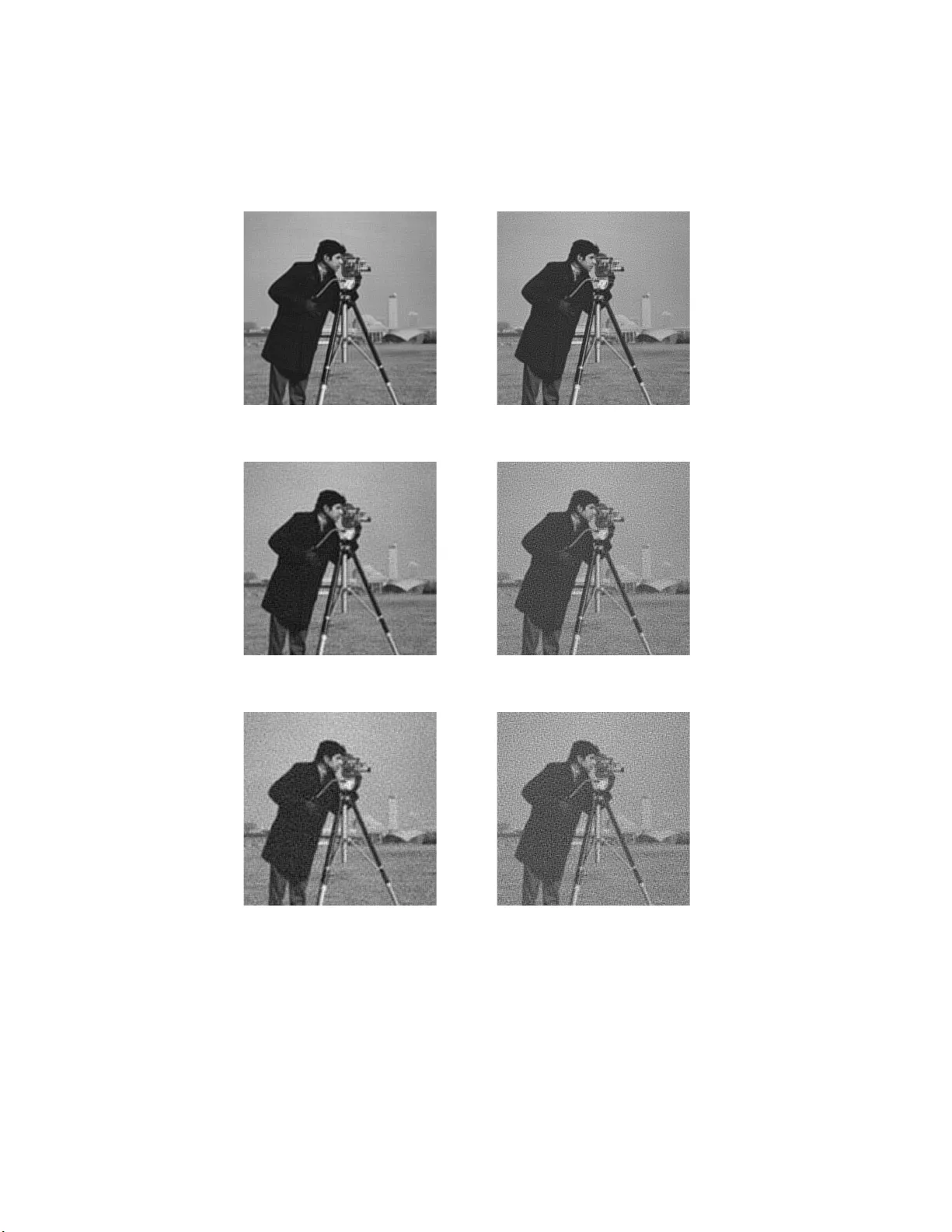
1 Generalized SURE for Exp onen tial F amilies: Applicati ons to Regularization Y onina C. Eldar Abstract Stein’s un biase d risk estimate (SURE) w as propo sed b y Stein for the independen t, identically distributed (iid) Gaussian mo del in order to derive estimates that dominate least-squares (LS). In recent y ears, the SURE criterion has been employ ed in a v ariety of denoising pro blems for choosing regular ization parameters that minimize an estimate of t he mean-squa red error (MSE). How ever, its use has been limited to the iid case whic h precludes many impo r tant applications. In this pap er we begin by deriving a SURE count er pa rt for general, not necessar ily iid distributions fro m the exp onential family . This enables extending the SURE design technique to a muc h bro ader class of problems. Based on this generalization w e suggest a new method for choosing regula r ization para meters in p enalized LS estimators . W e then demonstrate its sup erior p erfor mance ov er the conven tiona l generalized cross v alidation approach and the discrepancy method in the conte xt of image deblurr ing and deconvolution. The SURE tech nique can also b e used to design estimates without predefining their structure. Ho wev er , allowing for too many free parameters impairs the p e rformance of the resulting estimates. T o addre s s this inherent tra deo ff we pr op ose a regularized SURE ob jective. Based on this design criterion, w e derive a w av elet denoising strategy that is similar in sprit to the standard s oft-threshold approa ch but can lea d to impr ov ed MSE per formance. I. Introduction Estimation in multiv ariate p r oblems is a fundamental topic in statistical signal pro cessing. One of the m ost common r eco very strategie s for deterministic u nkno wn parameters is the we ll-kno wn maxim um lik eliho o d (ML) method. The ML estimat or enjoys sev eral app ealing prop erties, in clud ing asymptoti c efficiency under suitable regularit y conditions. Nonetheless, its mean-squared err or (MSE) can b e impro ved up on in the non-asymptotic regime in many differen t settings. Department of Electrical Engineering, T ec hn ion—I srael In stitute of T echnology , Haifa 32000, Israel. Phone: +972-4-8293256, fax: +972-4-8295 757, E-mail: yonina @ee.technion.ac.i l. This w ork was supp orted in part by t he Israel Science F oundation under Gran t no. 1081/07 and b y the Europ ean Commission in th e framewo rk of the FP7 Netw ork of Excellence in Wireless COMm unications NEWCOM++ (contract no. 21671 5). 2 In their seminal w ork, Stein and J ames sh o w ed that for the indep en d en t, identic ally-distributed (iid) linear Gaussian mo del, it is p ossible to construct a nonlinear estimator with lo wer MSE than that of ML f or all v alues of the un kno wns [1], [2]. V arious mo difications of the James-Stein metho d h a v e since b een dev elop ed that are app licable to the non-iid Gaussian case as well [3], [4], [5], [6], [7], [8]. The James-Ste in approac h is based on the Stein unbiased risk estimate (SURE) [9], [10], wh ich is an unbiase d estimate of the MSE. Sin ce the MSE in general dep end s on the true unkno wn parameter v alues it cann ot b e used as a design ob jectiv e. Ho wev er, using the S URE principle leads to a relativ ely simple tec hn ique for determining metho ds that ha v e lo w er MSE than ML. The idea is to c ho ose a class of estimate s, and then select the memb er from the class that minimizes the S URE estimate of the MSE. This strategy h as b een applied to a v ariet y of different denoising tec hn iques [11], [12], [13], [14 ]. Typically , in these problems, implicit prior information on the signal to b e r eco vered is incorp orate d in to the chosen structure of the estimate. F or example, in wa v elet denoising the signal is assum ed to b e sp ars e in the wa vele t domain whic h motiv es th e use of thresholding. Only the v alue of the threshold is determined by the SURE principle. The SURE metho d is app ealing as it allo ws to directly app ro ximate the MSE of an estimate fr om the data, without requir in g kn o wledge of the true parameter v alues. Ho w ev er, it h as t w o main dra wb ac ks whic h sev erely limit its u se in practical applications. The fir st restriction is that it w as originally limited to the iid Gaussian case. Sev eral extensions ha ve b een dev elop ed for d ifferent indep enden t mo dels. I n p articular, a SURE principle for iid, infi n itely d ivisible random v ariables with finite v ariance is deriv ed in [15 ]. Extensions to indep enden t v ariables from a con tin uous exp onentia l family are treated in [16], [17], w hile the discrete exp onent ial case is d iscussed in [18]. All of these generalizations are confin ed to the in dep endent case which precludes a v ariet y of imp ortant applications su c h as image deblur ring. The second dr a wbac k of using SURE as a design criterion is that in order to get m eaningful estimators the basic structure of the estima te must b e determined in adv ance. If no parametrization is assumed, then there are to o man y free v ariables to b e optimized, and the SURE metho d will typica lly not lead to go o d MSE b eha vior. In this pap er w e extend the basic SURE principle in t wo directions, in order to circum v en t the t wo fund amen- tal dra wbac ks outlined ab o v e. First, we generalize SURE to multiv ariate, p ossibly non-iid exp onen tial f amilies. 3 In particular, we dev elop an u n biased estimate of the MSE for a general Gaussian vecto r mo del. Exp onen tial probabilit y densit y fu nctions (p dfs) play an imp ortant r ole in statistic s d ue to the Pitman-Koopm an-Darmois theorem [19], [20], [21], which states that among distribu tions whose domain d o es not v ary with the parame- ter b eing estimated, only in exp onen tial families is there a sufficien t statistic with b ound ed dimension as the sample size increases [22]. F urthermore, efficien t estimators exist only wh en the underlying mo del is exp o- nen tial. Ma ny kno w n d istributions are of the exp onen tial form, such as Gaussian, gamma, c hi-square, b eta, Diric h let, Bernoulli, binomial, m ultinomial, P oisson, and geomet ric distributions. Our result has imp ortan t practical v alue as it extends the app licabilit y of the SURE tec hnique to more general estimation mo dels, and in particular to scenarios in whic h the observ ations are dep endent. This is the situation, for example, when using ov ercomplete wa vele t transforms, and in image deblurring. In addition, w e deriv e results f or the case in whic h the mo del is r an k-d eficien t so that the p df dep end s only on a pro jection of th e parameter v ector. An immediate app licatio n of this extension is to the general linear Gaussian mo del. In this setup, w e seek to estimate a p arameter ve ctor θ from noisy , b lurred measurements x = H θ + w where w is a Gaussian noise vect or and H may b e rank deficient . One of the most p op u lar reco v ery strategi es in this con text is the regularized least -squares (LS) m etho d . In th is approac h, the estima te is designed to m inimize a r egularized LS ob jectiv e where t yp ical c hoices of p enalizati on are w eigh ted ℓ 2 or ℓ 1 norms. An imp ortant asp ect of this tec h nique, which significan tly impacts its p erf ormance, is selecting the regularization parameter. A v ariet y of differen t metho ds hav e b een p rop osed for this purp ose [24], [25], [26], [27], [28], [29], [30], [31]. When an ℓ 2 norm is us ed to p enalize the LS solution, the resulting estimat e is linear and is referred to as T ikh ono v regularizatio n. One of the most p opu lar regularizatio n selecti on method s in this con text is generalized cross- v alidation (GCV) [32]. When an ℓ 1 p enalt y is used, the resulting estima te is nonlinear so that app lying th e GCV app roac h is more complicated. An alternativ e c hoice is the d iscrepancy metho d in whic h th e parameter is c hosen suc h that the resulting data error is equal to the noise v ariance. Here, w e suggest an alternativ e strategy based on our extended S URE criterion. Sp ecifical ly , w e us e SURE to ev aluate the MSE of the p enalized solution for any c hoice of r egularizati on, and then select the v alue that minimizes the SURE estimate. T his allo ws SURE-based optimization of a broad class of d eblurring and decon v olution metho ds including b oth linear and non linear tec hniques. A similar app roac h wa s studied in 4 the sp ecia l case of Tikh on ov regularization with white n oise in [24 ], [25], [26]. Ho wev er, our tec hnique is not limited to an ℓ 2 p enalt y and can b e used with any other p enalized L S metho d . When the estimate is n ot giv en explicitly but rather as a solution of an optimiz ation p roblem w e can still emplo y the SURE strategy b y using a Mont e-Carlo appr oac h to appro ximate the d eriv ativ e of the estimate, which figures in the SURE expression [39]. Using sev eral test images and a decon vo lution problem, we demonstrate that this strategy often leads to significan t p erf orm ance impro veme nt ov er the standard GCV and discrepancy selectio n criteria in the conte xt of image deblurring and d econ v olution. Finally , to circumv ent the need for pre-defining a particular structure when app lying SURE, we prop ose an alternativ e approac h based on regularizing the SURE ob ject ive . Sp ecifically , we suggest adding a p enalizati on term to the SURE expr ession and c ho osing an estimate that minimizes the regularized function. In this wa y , w e can con trol the pr op erties of th e estimate without havi ng to a-priori assume a sp ecific structure. W e then illustrate this strategy in the conte xt of w av elet denoising. Instead of assuming a th r eshold estimate and c ho osing the thr esh old to minimize the SURE criterio n, as in [11], we d esign an estimate that minimizes an ℓ 1 regularized SURE ob jectiv e. The resulting denoising scheme has the form of a th reshold w ith a particular form of shrin k age, that is d ifferent than that obtained when using soft or h ard thresholding. T o ev aluate our metho d, w e compare it with Su reShrink of Donoho and Johnstone [11], by r ep eating the simula tions rep orted in their pap er. As we sho w, the r eco very results tend to b e b etter using our tec hnique. Moreo ver, our approac h is general as it is n ot tailored to a sp ecific p roblem. W e thus b eliev e that using a regularized SURE principle together with the generalized SURE deve lop ed h ere can extend the applicabilit y of SURE-based estimators to a br oad class of problems. The remaining of the pap er is organize d as follo ws. In Section I I w e introduce the b asic concept of MSE estimatio n. An extension of SURE to exp onenti al families is dev elop ed in Section I I I. In Section IV we discuss rank-deficien t mo dels in wh ic h the p df of the data dep end s only on a p ro jection of the u nkno wn parameter v ector. W e then sp ecialize the results to the linear Gaussian mo del in Section V. Applications to regularizat ion selection are discussed in Section VI. The regularized SURE criterion, together with an application to wa vel et denoising, are devel op ed in Section VI I. 5 I I. MSE Estima tion W e denote v ectors by b oldface lo we rcase letters, e.g. , x , and matrices b y b oldface upp ercase letters e.g., A . Th e i th comp onen t of a ve ctor y is written as y i , and ˆ ( · ) is an estimated vect or. The iden tit y matrix is written as I , A T is the transp ose of A , and A † denotes the pseudo-in v erse. F or a length- m v ector function h ( u ) ∈ R m of u ∈ R m , T r  ∂ h ( u ) ∂ u  = m X i =1 ∂ h i ( u ) ∂ u i . (1) W e consider the class of p roblems in which our goal is to estimate a d eterministic parameter v ector θ from observ ations x wh ich are related through a p df f ( x ; θ ). W e fu rther assume that the p df b elongs to the exp onent ial family of distributions and can b e expressed in the form f ( x ; θ ) = r ( x ) exp { θ T φ ( x ) − g ( θ ) } , (2) where r ( x ) and φ ( x ) are f unctions of the data only , and g ( θ ) dep ends on the unknown p arameter θ . As an example of an ap p licatio n w here the m o del (2) can o ccur, consider the lo cation problem of estimat ing a p arameter vec tor θ ∈ R m from observ ations x ∈ R n related through the linear mo d el: x = H θ + w , (3) where w is a zero-mea n Gaussian random v ector with co v ariance C ≻ 0. The p df of x is then giv en by (2) with r ( x ) = 1 √ (2 π ) n det( C ) exp {− (1 / 2) x T C − 1 x } ; φ ( x ) = H T C − 1 x ; g ( θ ) = (1 / 2) θ T H T C − 1 H θ . (4) Other examples of d istributions in the exp onen tial family include Po isson with u nkno wn mean, exp onentia l with u n kno wn mean, gamma, and Bernoulli or binomial with u nkno wn su ccess p robabilities. 6 Giv en the mo del (2), a sufficien t statistic for estimating θ is giv en by u = φ ( x ) . (5) Therefore, an y reasonable estimate of x will b e a fu nction only of u . More sp ecifically , from the Rao-Blac kwell theorem [33] it follo ws that if ˆ θ is an estimate of θ whic h is n ot a fu nction only of u , then the estimate E { ˆ θ | u } has lesser or equal MSE than that of ˆ θ , for all θ . Th erefore, in the sequel, we only consider method s that dep end on the d ata via u . Let ˆ θ b e an arbitrary estimate of θ , whic h we w ould lik e to design to minimize the MSE, defined by E {k ˆ θ − θ k 2 } . In practice, ˆ θ = h ( u ) where h ( u ) is some function of u that is t ypically c hosen to ha v e a particular structure, parameterized b y a v ector α . F or example, h ( u ) = α u where α is a scalar, or h i ( u ) = ψ α ( u i ) w here ψ α ( u ) = sign( u )[ | u | − α ] + (6) is a soft-threshold with cut-off α . Id eally , we w ould like to select α to minimize the MSE. Sin ce this is imp ossible, as we show b elo w, instead in the SURE approac h α is designed to minimize an u n biased estimate (referred to as the SURE estimate) of the MSE. W e can expr ess the MSE of ˆ θ = h ( u ) as E n k ˆ θ − θ k 2 o = k θ k 2 + E  k h ( u ) k 2  − 2 E  h T ( u ) θ  . (7) In order to minimize the MSE ov er h ( u ) w e need to explicitly ev aluate the expression v ( h , θ ) = E  k h ( u ) k 2  − 2 E  h T ( u ) θ  . (8) Eviden tly , the MSE will d ep end in general on θ , whic h is un kn o wn, and therefore cannot b e minimized. Instead, we ma y seek an unbiase d estimate of v ( h , θ ) and then c ho ose h to minimize this estimate. The d ifficult expression to appro ximate is E { h T ( u ) θ } as the dep endency on θ is explicit. Therefore, w e concen trate on estimating this term. If this can b e don e, then we can easily obtain an un biased MSE estimate. Sp ecifically , 7 supp ose we construct a fu nction g ( h ( u )) that dep end s only on u (and not on θ ), suc h that E { g ( h ( u )) } = E  h T ( u ) θ  △ = E h , θ . (9) Then ˆ v ( h ) = k h ( u ) k 2 − 2 g ( h ( u )) , (10) is an u n biased estimate of v ( h , θ ), since clearly E { ˆ v ( h ) } = v ( h , θ ). A reasonable strategy therefore is to select h ( u ) to m in imize our assessment ˆ v ( h ) of th e MSE. T his approac h w as first p r op osed b y Stein in [9], [10] for the iid Gaussian mo d el (3) with C = I and H = I . The d esign framewo rk prop osed ab o ve reduces to fin ding an u n biased estimat e of E h , θ . Clearly , any su c h appro ximation will d ep end on the p df f ( x ; θ ). In the next section we devel op an unbiase d estimate w hen the p df is give n by the exp onent ial mo del (2). Before addressing the general setting, to ease the exp osition we illustrate the main idea p rop osed by Stein, by fir st considering th e simpler iid Gaussian case. In this setting w e seek to estimat e a v ector θ ∈ R m from measurements x = θ + w , wh ere w is a zero-mean Gaussian random v ector with iid comp onen ts of v ariance σ 2 . In Section IV we treat the more d ifficu lt case in wh ic h u lies in a subspace A of R m , and the p df (2) d ep ends on θ only through its orthogo nal pr o jectio n on to A . Th is situation arises, for example, in the linear Gaussian mo del (3) when H is rank deficient . F or this setup , w e dev elop a SURE estimate of the MSE in estimating the p ro jected parameter. In S ections V and VI we consider several examples of estimates in whic h the free parameters are c hosen to minimize the SURE ob jectiv e. In particular, w e prop ose alternativ es to the p opular GCV and discrepancy metho ds for regularization. In Section VI I, w e suggest a r egularized SURE strategy for d etermining h ( u ) without the need for parametrization, and demonstrate its p erformance in the cont ext of w av elet denoising. 8 I I I. Extended SURE Principle A. IID Gaussian M o del W e b egin our deve lopment by treating the iid Gaussian setting . Since from (4), u = (1 /σ 2 ) x , we consider estimates ˆ θ = h ( x ) that are a f u nction of x . T o dev elop an unbiase d estimate of E h , θ , w e exploit the fact that for the Gaussian p df f ( x ; θ ) ( x i − θ i ) f ( x ; θ ) = − σ 2 ∂ f ( x ; θ ) ∂ x i . (11) Assuming th at E {| h i ( x ) |} is b ounded and h i ( x ) is weakly differen tiable 1 in x , w e hav e that E h , θ = m X i =1 Z ∞ −∞ h i ( x ) θ i f ( x ; θ ) d x = m X i =1 Z ∞ −∞ h i ( x )  x i f ( x ; θ ) + σ 2 ∂ f ( x ; θ ) ∂ x i  d x = E { h T ( x ) x } + σ 2 m X i =1 Z ∞ −∞ h i ( x ) ∂ f ( x ; θ ) ∂ x i d x , (12) where the second equalit y is a result of (11). T o ev aluate the second term in (12), we us e in tegration by parts: Z ∞ −∞ h i ( x ) ∂ f ( x ; θ ) ∂ x i d x = − Z ∞ −∞ h ′ i ( x ) f i ( x ; θ ) d x = − E { h ′ i ( x ) } , (13) w ere we denoted h ′ i ( x ) = ∂ h i ( x ) /∂ x i , and used the f act that | h i ( x ) f ( x ; θ ) | → 0 f or | x i | → ∞ since E {| h i ( x ) |} is b ound ed. W e conclude from (12) and (13) that E h , θ = − σ 2 m X i =1 E { h ′ i ( x ) } + E { h T ( x ) x } , (14) and th erefore, − σ 2 m X i =1 ∂ h i ( x ) ∂ x i + h T ( x ) x (15) 1 Roughly sp eaking, a function is weakly d ifferen tiable if it has a deriv ative almost ever y where, as long as the p oin ts that are not differentia ble are not delta functions; see [34] for a more formal definition. 9 is an u nbiased estimate of E h , θ . B. Extende d SURE W e no w extend th e basic approac h outlined in the previous section to the general class of exp onen tial p dfs. In order to address this mo del, we only consider metho ds that dep end on the data via u . T his enables the use of integ ration b y parts, similar to the iid Gaussian setting. The follo wing theorem p r o vides an unbiased estimate of E  h T ( u ) θ  whic h dep en d s only on u and not on the unknown p arameters θ . The or em 1: Let x denote a random v ector with exp onential p df given b y (2), and let u = φ ( x ) b e a sufficien t statistic for estimating θ from x . Let h ( u ) b e an arbitrary function of θ that is w eakly differen tiable in u and suc h that E {| h i ( u ) |} is b ounded. Then E  h T ( u ) θ  = − E  T r  ∂ h ( u ) ∂ u  − E  h T ( u ) ∂ ln q ( u ) ∂ u  , (16) where q ( u ) = Z r ( x ) δ ( u − φ ( x )) d x , (17) and δ ( x ) is the Kronec ker delta fun ction. Note, that as we show in the pro of of the theorem, the p df f ( u ; θ ) of u is giv en by f ( u ; θ ) = q ( u ) exp { θ T u − g ( θ ) } . (18) Therefore, an alternativ e to computing q ( u ) u s ing (17) is to ev aluate the p df of u and then use (18). F rom the theorem, it follo ws th at − T r  ∂ h ( u ) ∂ u  − h T ( u ) ∂ ln q ( u ) ∂ u (19) 10 is an u nbiased estimate of E { h T ( u ) θ } . In the iid Gaussian case, u = (1 /σ 2 ) x so that ∂ h ( u ) ∂ u = σ 2 ∂ h ( x ) ∂ x . (20) F urthermore, u is a Gaussian iid vec tor with elemen ts that hav e mean (1 /σ 2 ) θ and v ariance 1 /σ 2 so that q ( u ), whic h is the n ormalizatio n factor, is giv en b y q ( u ) = K exp {−k u k 2 σ 2 / 2 } for a constan t K . Consequen tly ∂ ln q ( u ) ∂ u = − σ 2 u = − x . (21) Substituting (20) and (21) in to (19), the estimate reduces to (15), derive d in the iid Gaussian setting. Pr o of: T o prov e th e theorem we first determine the p df of u . S in ce u = φ ( x ) we ha ve that [33, p. 127] f ( u ; θ ) = Z f ( x ; θ ) δ ( u − φ ( x )) d x . (22) Substituting (2 ) into (22), f ( u ; θ ) = exp { θ T u − g ( θ ) } Z r ( x ) δ ( u − φ ( x )) d x = q ( u ) exp { θ T u − g ( θ ) } . (23) No w, E  h T ( u ) θ  = = Z h T ( u ) θ exp { θ T u − g ( θ ) } q ( u ) d u = m X i =1 Z h i ( u ) θ i exp { θ T u − g ( θ ) } q ( u ) d u . (24) Noting that θ i exp { θ T u − g ( θ ) } = ∂ exp { θ T u − g ( θ ) } ∂ u i , (25) 11 w e hav e Z ∞ −∞ h i ( u ) θ i exp { θ T u − g ( θ ) } q ( u ) du i = = Z ∞ −∞ h i ( u ) q ( u ) ∂ exp { θ T u − g ( θ ) } ∂ u i du i = − Z ∞ −∞ ∂ h i ( u ) q ( u ) ∂ u i exp { θ T u − g ( θ ) } du i , (26) where w e u sed the fact that | h i ( u ) q ( u ) exp { θ T u − g ( θ ) }| → 0 for | u i | → ∞ sin ce E {| h i ( u ) |} is b oun d ed. No w, ∂ h i ( u ) q ( u ) ∂ u i = ∂ h i ( u ) ∂ u i q ( u ) + ∂ q ( u ) ∂ u i h i ( u ) . (27) Substituting (26) and (27) in to (24), E  h T ( u ) θ  = = − m X i =1 Z ∂ h i ( u ) q ( u ) ∂ u i exp { θ T u − g ( θ ) } ∂ u = m X i =1  − E  ∂ h i ( u ) ∂ u i  − E  ∂ q ( u ) ∂ u i h i ( u ) q ( u )  = − E  T r  ∂ h ( u ) ∂ u  − E  h T ( u ) ∂ ln q ( u ) ∂ u  , (28) whic h completes the pro of of the theorem. Based on Theorem 1 we can deve lop a general ized S URE principle for estimating an unkno wn parameter v ector θ in an exp onent ial m o del. Sp ecifically , let ˆ θ = h ( u ) b e an arb itrary estimate of θ based on the data x , where h ( u ) satisfies the regularit y conditions of Theorem 1. Com bining (7) and T h eorem 1, an unbiase d estimate of the MSE of ˆ θ is giv en by S ( h ) = k θ k 2 + k h ( u ) k 2 + 2 T r  ∂ h ( u ) ∂ u  + 2 h T ( u ) ∂ ln q ( u ) ∂ u . (29) W e ma y then design ˆ θ b y c ho osing h ( u ) to minimize S ( h ). 12 In the iid Gaussian case, (29) reduces to k θ k 2 + k h ( x ) k 2 + 2 σ 2 ∂ h ( x ) ∂ x − 2 h T ( x ) x (30) where we used the fact that u = (1 /σ 2 ) x whic h imp lies ∂ ln q ( u ) /∂ u = − x , and ∂ h ( u ) /∂ u = σ 2 ∂ h ( x ) /∂ x . The MSE estimate (30) wa s fi r st prop osed b y Stein 2 in [9], [10]. The SURE estimate can b e used to determine un kno wn regularization parameters which comprise a giv en estimatio n s trategy . An example is the SureS h rink approac h to wa ve let denoising [11]. Extending th is tec h- nique, our general SURE ob jectiv e (29) ma y b e used to select regularization parameters in more general mo dels. W e discuss these ideas in the cont ext of linear Gaussian p roblems in Section V. IV. Rank-Deficient Models In some settings, the sufficien t statistic u lies in a subspace A of R m . As an example, supp ose that in the Gaussian mo del (3) H is rank-deficien t. In this case u = H T C − 1 x lies in the range space R ( H T ) of H T , whic h is a sub space of R m . If θ is not restricted to a subsp ace, then we d o not expect to b e able to r eliably estimate θ fr om u , unless some additional information on θ is kno wn. No netheless, we ma y still obtain a reliable assessmen t of the part of θ that lies in A . Denote by P the orthogonal pro jectio n on to A . Th en , we sho w b elo w, that if u dep ends on θ only through P θ , and in addition u has an exp onentia l p df, then we can obtain a SURE estimate of the error in A , namely E {k P ˆ θ − P θ k 2 } . If in addition ˆ θ lies in A , th en up to a constan t, indep enden t of ˆ θ , this appro ximation is also an unbiase d estimate of the tru e MSE E {k ˆ θ − θ k 2 } . T o deriv e the SURE estimate in this case, w e fir st note that if u lies in A , then θ T u = ( P θ ) T ( Pu ) . (31) Supp ose that A has d imension r < m . Since P θ lies in an r -d imensional sp ace, it can b e expressed in terms of r comp onen ts in an appropr iate basis. Denoting by V an m × r matrix with orthonormal v ectors that span 2 W e note that the expression obtained b y Stein is sligh tly different since instead of optimizing ˆ θ = h ( x ) , h e considered estimates of the form ˆ θ = x + h ( x ) and then optimized h ( x ). The t wo expressions differ by a constant, which does not effect the optimization of h ( x ). 13 A = R ( P ), the vect or P θ can b e expressed as P θ = V θ ′ for an appropriate length- r v ector θ ′ . S imilarly , Pu = V u ′ . Therefore, w e can write θ T u = θ ′ T u ′ , (32) where w e used the fact that V T V = I . W e assume that u ′ is a su fficien t statistic for θ ′ and that f ( u ′ ; θ ′ ) has an exp onen tial p df: f ( u ′ ; θ ′ ) = q ( u ′ ) exp { θ ′ T u ′ − g ( θ ′ ) } . (33) Under this assum p tion, we next derive a SURE estimate of th e MSE in A . The MSE in estimating θ can then b e written as E {k ˆ θ − θ k 2 } = E {k P ˆ θ − P θ k 2 } + E {k ( I − P ) ˆ θ − ( I − P ) θ k 2 } . (34) If ˆ θ lies in A , then ( I − P ) ˆ θ = 0 and the second term is constant , indep enden t of ˆ θ . Therefore, in this case, to optimize ˆ θ it is su fficien t to obtain an un biased estimate of the first term. As w e sh o w b elo w, such an assessmen t can b e d eriv ed using similar ideas to those in T heorem 1. Even if ˆ θ do es not lie in A , th e SURE estimate w e dev elop ma y b e u sed to appr oximat e the first term. Since u dep ends only on P θ , it is reasonable to restrict atte ntio n to estimates ˆ θ = h α ( u ) where the parameters α are tuned to minimize the MSE in A E {k P ˆ θ − P θ k 2 } , sub j ect to any other p rior information w e ma y ha ve , such as norm constrain ts on θ . In suc h cases w e can use a regularized SURE criterion with th e SURE ob jectiv e b eing the MSE in A , as we discuss in S ection VI I. W e n ow deve lop a SURE estimate of the MSE E {k P ˆ θ − P θ k 2 } . T o this end we need to find an unbiase d estimate of E { ˆ θ T P θ } = E { ˆ θ T V θ ′ } = E { ( V T ˆ θ ) T θ ′ } (3 5) Let ˆ θ = h ( u ) = h ( u ′ ) (since u = V u ′ , it is clear that ˆ θ is a function of u ′ ). By our assumption, θ ′ has an exp onent ial p d f with su fficien t stati stic u ′ . Therefore, w e can app ly Theorem 1 to V T h ( u ) for an y function 14 h ( u ) that ob eys the conditions of th e th eorem, wh ic h yields E  h T ( u ) V θ ′  = − E  T r  V T ∂ h ( u ′ ) ∂ u ′  − E  h T ( u ′ ) V ∂ ln q ( u ′ ) ∂ u ′  = − E  T r  P ∂ h ( u ) ∂ u  − E  h T ( u ) V ∂ ln q ( u ′ ) ∂ u ′  , (36) where we used the fact that P = VV T and ∂ h ( u ′ ) ∂ u ′ = ∂ h ( u ) ∂ u V . (3 7) W e conclude that if h ( u ) is an estimate of a parameter v ector θ , w here u lies in a subsp ace A and is a sufficien t statistic for estimating P θ , with P denoting the orthogonal p ro jection onto A , then an unbiased estimate of the MSE E {k Ph ( u ) − P θ k 2 } is giv en by S ( h ) = k P θ k 2 + k Ph ( u ) k 2 + 2 T r  P ∂ h ( u ) ∂ u  + 2 h T ( u ) V ∂ ln q ( u ′ ) ∂ u ′ , ( 38) with u = V u ′ and V denoting an orthonormal b asis f or A . When A = R m , P = I , V = I and (38) redu ces to (29). V. Linear Ga us sian Model W e no w sp ecialize the SURE principle to the linear Gaussian model (3). W e b egin by treating the case in whic h H is an n × m matrix with n ≥ m and full column rank. W e then discuss the rank-deficien t scenario. A. F ul l-R ank Mo del T o u se Theorem 1 we n eed to compu te the p df q ( u ) of u . S in ce u = H T C − 1 x , it is a Gaussian random v ector w ith mean H T C − 1 H θ and co v ariance H T C − 1 H . As q ( u ) is the f u nction m ultiplying th e exp onentia l in the p df of u , it follo ws f r om (4) that q ( u ) = K exp {− (1 / 2) u T ( H T C − 1 H ) − 1 u } , (39) 15 where K is a constan t, ind ep endent of u . Therefore, ∂ ln q ( u ) ∂ u = − ( H T C − 1 H ) − 1 u = − ˆ θ ML , (40) where ˆ θ ML is the ML estimate of θ giv en b y ˆ θ ML = ( H T C − 1 H ) − 1 H T C − 1 x . (41) It then follo ws from Theorem 1 th at E  h T ( u ) θ  = − E  T r  ∂ h ( u ) d u  − h T ( u ) ˆ θ ML  . (42) Using (29) and (40) w e conclude that S ( h ) = k θ k 2 + k h ( u ) k 2 + 2  T r  ∂ h ( u ) ∂ u  − h T ( u ) ˆ θ ML  , (43) is an u nbiased estimate of the MSE. B. R ank- D eficient Mo del Next, w e consider the linear Gaussian mo d el (3) with a r ank-deficient H . Supp ose that H has a singular v alue decomp osition H = U Σ Q T for some un itary matrices U and Q . Let H ha ve r ank r so th at Σ is a diagonal n × m matrix wh at the first r d iagonal elemen ts equal to σ i > 0 and the remaining ele ments equal 0. In this case, V is equal to the fir st r columns of Q and θ ′ = V T θ . A sufficien t statisti c for estimating θ ′ is u ′ = V T H T C − 1 x . Indeed, u ′ is a Gaussian random vect or with mean µ ′ = V T H T C − 1 H θ and co v ariance C ′ = V T H T C − 1 HV . Using the SVD of H we h a v e that µ ′ = Λ[ U T C − 1 U ] r θ ′ , C ′ = Λ[ U T C − 1 U ] r , (44) 16 where Λ is an r × r diagonal matrix w ith diagonal elemen ts σ 2 i > 0 and [ A ] r is the r × r top-left pr inciple blo c k of size r of the matrix A . Since C ≻ 0, C ′ is in ve rtible. Therefore, f ( u ′ ; θ ′ ) = q ( u ′ ) exp { θ ′ u ′ − g ( θ ′ ) } (45) with q ( u ′ ) = 1 √ (2 π ) n det( C ′ ) exp {− (1 / 2) u ′ T C ′− 1 u ′ } ; g ( θ ′ ) = (1 / 2) θ ′ T Λ[ U T C − 1 U ] r θ ′ . (46) W e therefore conclude from (38) that an u n biased estimate of th e MSE E {k Ph ( u ) − P θ k 2 } is giv en b y k P θ k 2 + k Ph ( u ) k 2 + 2  T r  P ∂ h ( u ) ∂ u  − h T ( u ) ˆ θ ML  , (47) where ˆ θ ML = ( H T C − 1 H ) † H T C − 1 x is an ML estimate . Here w e used the fact that V C ′− 1 u ′ = ( H T C − 1 H ) † H T C − 1 x . W e summarize our r esu lts for the linear Gaussian mo del in the follo wing prop osition. Pr op osition 1: Let x d en ote measur emen ts of an un kno wn parameter ve ctor θ in the linear Gaussian mo del (3), where w is a zero-mean Gaussian random v ector with co v ariance C ≻ 0. Let h ( u ) with u = H T C − 1 x b e an arbitrary fu nction of θ that is w eakly differen tiable in u and su c h that E {| h i ( u ) |} is b ounded, and let P b e an orthogonal pr o jectio n on to R ( H T ). Then E  h T ( u ) P θ  = − E  T r  P ∂ h ( u ) ∂ u  − h T ( u ) ˆ θ ML  , where ˆ θ ML = ( H T C − 1 H ) † H T C − 1 x 17 is an ML estimate of θ . An u nbiased estimate of the MSE E {k Ph ( u ) − P θ k 2 } is S ( h ) = k P θ k 2 + k Ph ( u ) k 2 + 2  T r  P ∂ h ( u ) ∂ u  − h T ( u ) ˆ θ ML  . (48) C. Examples T o illustrate the us e of the SURE principle, s u pp ose that we consider estimators of the form ˆ θ = α ˆ θ ML where ˆ θ ML is giv en b y (41), and we wo uld lik e to select a go o d c hoice of α . T o this end, we minimize the S URE unbia sed estimate of the MSE giv en by Prop osition 1 with h ( u ) = α ˆ θ ML . Note that in this case h ( u ) ∈ R ( H T ) so that S ( h ) + k ( I − P ) θ k 2 is an unbiased estimate of the total MSE E {k ˆ θ − θ k 2 } and therefore it suffices to minimize S ( h ). F or this choi ce of h ( u ), minimizing S ( h ) is equiv alen t to minimizing α 2 k ˆ θ ML k 2 + 2  α T r  ( H T C − 1 H ) †  − α k ˆ θ ML k 2  . (49) The optimal c hoice of α is α = 1 − T r  ( H T C − 1 H ) †  k ˆ θ ML k 2 , (50) resulting in ˆ θ = 1 − T r  ( H T C − 1 H ) †  k ˆ θ ML k 2 ! ˆ θ ML . (51) The estimate of (51) coincides with the balanced blind m in imax metho d prop osed in [7, E q. (45)], wh ic h w as deriv ed based on a minimax fr amew ork [8]. Here we see that the same tec hnique resu lts from applying our generaliz ed SURE criterion. A striking feature of this estimate, pro ve d in [7], is that when H T C − 1 H is in ve rtible and its effectiv e d imension is larger than 4, it dominates ML for all v alues of θ (see Theorem 3 in [7]). This m eans that its MSE is alwa ys lo wer than that of the ML metho d , regardless of the true v alue of θ . When H = I and C = σ 2 I , (51) redu ces to ˆ θ =  1 − nσ 2 k x k 2  x , (52) 18 whic h coincides with Stein’s estimate [1]. This tec hnique is kno wn to dominate ML f or n ≥ 3. If in addition we require that α ≥ 0, then the estimate of (51) b ecomes ˆ θ = " 1 − T r  ( H T C − 1 H ) †  k ˆ θ ML k 2 # + ˆ θ ML , (53) where we used the notation [ x ] + =        x, x ≥ 0; 0 , x < 0 . (54) The method of (53) is a p ositiv e-part v ersion of (51 ). In the iid case, it redu ces to the p ositiv e-part S tein’s estimate [35], which is kno wn to dominate the standard S tein approac h (52). Next, consider the case in wh ic h H = I and C = D with D = diag ( σ 2 1 , . . . , σ 2 n ) and sup p ose w e seek a diagonal estimate of the form ˆ θ i = α i x i . Minimizing the un biased esti mate of (48) in this case is equiv alent to min imizing n X i =1 α 2 i x 2 i + 2 n X i =1 σ 2 i α i − 2 n X i =1 α i x 2 i , (55 ) whic h yields α i = 1 − σ 2 i x 2 i . (56) Restricting th e co efficien ts α i to b e non-negativ e leads to the estimate ˆ θ i =  1 − σ 2 i x 2 i  + x i . (57) In con trast to ˆ θ of (51), whic h dominates the ML metho d, it can b e prov en that the estimate of (57) is not d ominating. T h us, we see that b y allo wing for to o m an y fr ee parameters, we impair the p erformance of the SURE-based estimate. On the other hand , assuming strong structure, as in (51), sev erely restricts the class of estimators and consequently limits the p ossible p erformance adv an tage whic h can b e obtained. In Section VI I w e suggest a regularized SURE strategy in order to o v ercome this inheren t tradeoff b et ween o v er-parametrization and p erf ormance. 19 VI. Applica tion to Regulariza tion Selec tion A p opular strategy for solving in verse problems of the form (3) is to use regularizat ion tec hniques in conjunction with a LS ob jectiv e. Sp ecifically , the estimate ˆ θ is c hosen to minimize a regularized LS criterion: ( x − H ˆ θ ) C − 1 ( x − H ˆ θ ) + λ k L ˆ θ k (58) where the norm is arbitrary . Here L is some regularizatio n op erator suc h as the discretizat ion of a first or second ord er different ial op erator that account s for smo othness prop erties of θ , and λ is the regularizati on parameter [28], [27]. An imp ortan t problem in p ractice is the select ion of λ , which strongly effects the reco very p erformance. One of the most p opular app roac h es to c ho osing λ when the estimate is linear (as is the case when a squared- ℓ 2 norm is used in (58)) is the generaliz ed cross-v alidation (GCV) metho d [32]. When the estimate tak es on a more complicated n on linear form, a p opular selection metho d is the d iscrepancy principle [26]. Based on our generalized SURE criterion, we choose λ to minimize the SURE ob jectiv e (48 ). As we demonstrate for the cases in whic h the norm in (58) is the squared- ℓ 2 or ℓ 1 norms, this m etho d can dramatical ly outp erform GCV and the discrepancy tec h nique in pr actica l applica tions. A. Image Deblurring W e first consider th e case in whic h the squared- ℓ 2 norm is used in (58). The s olution then has the form ˆ θ = ( Q + λ L T L ) − 1 H T C − 1 x , (59) where for br evit y w e d enoted Q = H T C − 1 H . (60) The estimate (59) is commonly r eferred to as Tikhonov regularizatio n [23]. 20 In the GCV metho d, λ is c hosen to minimize G ( λ ) = 1 T r 2 ( I − ( Q + λ L T L ) − 1 Q ) n X i =1 ( x i − [ H ˆ θ ] i ) 2 . (61) The SURE c hoice follo ws d irectly from minimizing (48). In our s imulatio ns b elo w, b oth min imizations where p erformed b y using the fmincon fu nction on Matlab. T o demonstrate the p erformance of th e prop osed regularizatio n metho d, w e tested it in the con text of image d eb lu rring u s ing the HNO d eblurring p ac k age for Matlab 3 based on [36]. W e c hose several test images, and blurred them u sing a Gaussian p oint- sp r ead f u nction of dimens ion 9 with standard deviation 6 using the function p sfGauss . W e then added zero-mean, Gaussian white noise with v ariance σ 2 . In Figs. 1 and 2 w e compare the deblur red images resulting f rom using the Tikhono v estimate (59) with L = I where th e regularizatio n parameter is chosen according to our new SURE criterion (left) and the GCV metho d (right ), for different noise lev els. As can b e seen from the figur es, our S URE based app r oac h leads to a su bstan tial p erformance improv ement o v er the standard GCV criterion. This can also b e s een in T ables I and I I in which we r ep ort the resulting MSE v alues. T ABLE I MSE f or Tikhonov De blurring of Lena σ = 0 . 01 σ = 0 . 05 σ = 0 . 1 GCV 0.0022 0.0077 0.0 133 SURE 0.0011 0.0025 0.0 042 T ABLE I I MSE f or Tikhonov De blurring of Cameraman σ = 0 . 01 σ = 0 . 05 σ = 0 . 1 GCV 0.0033 0.0121 0.0 221 SURE 0.0016 0.0039 0.0 064 3 The pac k age is a v ailable at http://www2. imm.dtu.dk/~pch/H N O/ . 21 B. De c onvolution Example As another applicatio n of the S URE, consider the standard decon vo lution problem in which a signal θ [ ℓ ] is con vo lve d b y an impulse resp onse h [ ℓ ] and cont aminated by additiv e white Gaussian noise with v ariance σ 2 . The obs erv ations x [ ℓ ] can b e w ritten in the form of the linear mo del (3) wh ere x is the vec tor con taining the observ ations x [ ℓ ], θ consists of the input signal θ [ ℓ ], and H is a T o eplitz matrix, represen ting con v olution with the imp u lse resp onse h [ ℓ ]. T o reco ver θ [ ℓ ] w e may use a p enalized LS app roac h (58) where w e assume that the original signal θ [ ℓ ] is smo oth. This can b e accoun ted for by c h o osing a p enalization of the form k L θ k 1 where L repr esen ts a second order deriv ativ e op erator. The r esulting p enalized LS estimate can b e determined by solving a quadratic optimizatio n problem. In our sim ulations, w e used C VX , a p ac k age for sp ecifying and solving con vex programs in Matlab [37]. Since the r esulting estimate is n on -linear, d ue to the ℓ 1 p enalization, we cannot apply the GCV equati on (61). In stead, a p opular approac h to tune the parameter λ is to use the discrepancy principle in whic h λ is c hosen such that the r esidual k x − H ˆ θ k 2 is equal to the noise lev el nσ 2 [26], [25]. T o ev aluate the p erformance of the SURE prin ciple in this con text, w e consider an example from the Regularizati on T o ols [38] for Matlab. All the problems in this toolb ox are discretized v ersions of the F redholm in tegral equation of the first kind : g ( s ) = Z b a K ( s, t ) θ ( t ) dt (62) where K ( s, t ) is the k ernel and θ ( t ) is the solution f or a giv en g ( s ). The p r oblem is to estimate θ ( t ) from noisy samples of g ( s ). Using a midp oin t rule with n p oint s, (62) reduces to an n × n linear system x T = H θ . The fu nctions in th is toolb ox differ in K ( t, s ) and θ ( s ). Belo w we consider the fu n ction heat(n) w ith n = 80. The outpu t of the f unction is the matrix H a nd the true v ector θ (whic h represen ts θ ( t )). The observ ations are x = x T + w wh ere w is a white Gaussian n oise vect or with v ariance σ 2 = 1. In Fig. 3 w e plot the original signal along with the observ ations x , and the clean con vo lve d signal x T = H θ . The original signal along with the estimat es usin g the SURE principle and the discrepancy method are p lotted in Fig. 4. T o ev aluate the gradient of the estimate, we u sed the Mon te-Carlo SURE appr oac h p rop osed in 22 [39]. Eviden tly , the SURE metho d leads to sup erior p erformance. The MSE using the SURE appr oac h in this example is 0.10 wh ile the d iscrepancy strategy leads to an MSE of 1.16. VI I. Regularized SURE Method A crucial elemen t in guarante eing success of the SURE metho d is to c ho ose a go o d parameterization of h ( u ). How eve r, in many conte xts, suc h a structure ma y b e hard to find. O n the other hand, letting the SURE criterion select many free parameters can d eteriorate its p erformance. One w a y to treat this inherent tradeoff is b y regularizatio n. Thus, in stead of minimizing the SURE ob jectiv e w e suggest minimizing a regularized v ersion: S ( h , λ ) = S ( h ) + λr ( h ( u )) (63) where λ is a r egularizat ion parameter and r ( h ( u )) is a regularization fu nction. F or example, we ma y c h o ose r ( v ) = k v k where the norm is arbitrary . T he parameter λ is d etermined by app lying the con v enti onal SURE (29) (or (38)) to the estimate h ( u , λ ) resulting from solving (63) with λ fi xed. As an example, consider the iid Gaussian mo d el in w hic h x = θ + w where w is a Gaussian n oise ve ctor with iid zero-mean comp onen ts of v ariance σ 2 . Assuming that θ represent s the wa ve let co efficien ts of some underlying signal x , a p opular estimation strategy is w a ve let denoising in whic h eac h comp onent of x is replaced by a soft or h ard-thresholded v ersion. In particular, in their landmark pap er, Donoho and J ohnstone [11] d ev elop ed a soft-threshold w a vel et denoising m etho d in wh ich ˆ θ i =        | x i | − t, | x i | ≥ t ; 0 , | x i | < t, (64) where t is a threshold v alue. They suggest s electing t to minimize the SURE criterion, and refer to the resulting estimate as Sur eShrink (to b e more p r ecise, in Sur eShrink t is determined by SURE only if it lo we r than some upp er limit). In dev eloping the S u reShrink method, the function h ( x ) is r estricted to b e a comp onen t-wise soft th r eshold. The motiv ation for th is c h oice is that the wa v elet co efficient s b elo w a certain lev el tend to b e sparse. I t is w ell kno wn that soft-thresholding can b e obtained as the solution to a LS criterion with an ℓ 1 23 p enalt y: min  k x − θ k 2 + λ k θ k 1  . (65) Th us , in p rinciple w e can view the SureShr ink app r oac h as a 2-step pr o cedure: W e first determine the estimate that min imizes an ℓ 1 p enalized LS criterion. W e then c ho ose the p enaliza tion fact or to minimize SURE. Instead, we suggest c ho osing an estimate that directly m inimizes an ℓ 1 regularized SURE ob jectiv e, wh ere the only assumption we m ak e is that the pro cessing is p erformed comp onent wise. Th us , ˆ θ i = α i x i for some co efficients α i ( x ) ≥ 0. Since u = (1 /σ 2 ) x i , h i ( u ) = σ 2 α i u i . With this c hoice of h ( u ), minimizing (63) is equiv alen t to minimizing the follo w ing ob jectiv e: S ( α , λ ) = n X i =1 α 2 i x 2 i + 2 n X i =1 α i  σ 2 − x 2 i  + λ n X i =1 | α i || x i | . (66) The optimal c hoice of α i ≥ 0 is α i =  1 − σ 2 + λ | x i | x 2 i  + . (6 7) The resu lting estimate can b e viewed as a soft-thresholding method , with a particular c hoice of shrink age (differen t than the standard appr oac h (64)) wh en the v alue of x i exceeds the thr eshold. T he precise thr eshold v alue is equal to the largest v alue x i for wh ic h α i = 0 and is giv en by t = 1 2  λ + p λ 2 + 4 σ 2  . (68) T o c ho ose λ , w e su bstitute the estimate ˆ θ i = α i ( λ ) x i with α i ( λ ) giv en b y (67) int o the SURE criterion (48 ) with P = I , and min imize with resp ect to λ . The v alue of λ can b e easily determined numerical ly . T o demonstrate the adv antag e of our metho d o v er con v ent ional soft-thresholding we imp lemen ted our approac h on the examples tak en from [11]. Sp ecifically , we u sed the test functions Blo c ks, Bumps, Hea viS in e and Doppler defined in [11]. T he length of all signals is 2048 and the noise v ariance is σ 2 = 4. W e used the Daub ec hies 8 symmetrical wa v elet, and L = 5 lev els are considered. In T able I I I we rep ort the empirical MSE v alues of th e original noisy signals, and 3 w av elet d enoising sc hemes: Sur eS h rink w hic h is the metho d of [11] with the threshold selected u sing SURE, our prop osed regularize d SURE method (RSURE), and OracleShrink 24 whic h is a soft-threshold wh ere the thresh old v alue is selected to minimize the squared-error b et w een the true unknown wa v elet co efficien t, and its denoised v ersion. Clearly this approac h is only for comparison and serv es as a b enchmark on the b est p ossible p erformance that can b e obtained using an y soft thresh old. As can T ABLE I I I MSE f or Different So ft Denoising Schemes Blocks Bumps Hea viSine Dopp ler Original 4.054 4.072 4.153 3.945 SureShr ink 0.744 0.875 0.205 0.290 RSure 0.694 0.816 0.169 0.273 OracleShrink 0.690 0.828 0.118 0.283 b e s een from the table, the regularized S URE metho d p erform s b etter in all cases than Su reShrink. It is also in teresting to see that it sometimes ev en outp erforms Or acleShrink which is based on the true unknown θ . Th e reason the p erformance can b e b etter than the oracle is that the shr ink age p erformed in RSURE is differen t than the con v entio nal soft th r eshold. In T able IV we rep eat our exp erimen ts where now we use the estimates resulting fr om the standard S URE criterion. Sp ecifically , w e consider the p ositiv e-part Stein estimate (51) referred to as SteinShr in k and the estimate (57) whic h w e refer to as ScalarShrink. Eviden tly , using the SURE estimate without r egularizati on T ABLE IV MSE f or Different Denoising Schemes Blocks Bumps Hea viSine Doppler ScalarShrink 1.043 1.362 0.161 0.594 SteinShrink 1.681 1.730 1.508 1.413 deteriorates the p erformance significan tly . Thus, S URE alo ne is not generally sufficien t to obtain go o d esti- mates. Ho wev er, adding regularizati on dr amatical ly impro v es the b eha vior without the need to pre-sp ecify the desired str u cture. Finally , in T able V we r ep eat the exp eriments of T able I I I to determine the threshold v alues, but once the v alues are found we apply h ard-thresholding on the co efficien ts. As can b e seen from the table, ev en though the thresholding op eration is now the same in b oth metho ds, RSURE p erforms significan tly b ette r. Th us, the thr eshold determined from this metho d is sup erior to that resulting from th e SURE criterion without 25 T ABLE V MSE f or Different H ard-Thresholding Schemes Blocks Bumps Hea viSine Doppler SureShr ink 1.902 1.961 0.988 0.630 RSure 1.5 60 1.91 2 0.766 0.700 regularizatio n. Here again the imp ortance of r egularizat ion is demonstrated. VI I I. Conclusion In this pap er, w e d ev elop ed an un biased estimate of the MSE in multi v ariate exp onen tial families by ex- tending the SURE method . This generalized principle can n o w b e used in exp onen tial m ultiv ariate estimat ion problems to deve lop estimators with impro ved p erformance o ve r existing approac h es. As an app licatio n, we suggested a new strateg y for c ho osing the regularization parameter in p enalized in v erse problems. W e demon- strated via sev eral examples that this metho d can significan tly improv e the MSE o ve r the stand ard GCV and discrepancy approac hes. W e also suggested a regularized SURE criterion for selecting estimators w ithout the need for pre-sp ecifying their structure. Applying this ob jectiv e in the con text of wa ve let denoising, we pro- p osed a new t yp e of soft-thresholding whic h m in imizes a p enalized estimate of the MSE. As we demonstrated, this strategy can lead to impro ved MSE b ehavio r in comparison with soft and hard thresholding metho ds. The main con tribution of this w ork is in introd ucing the generali zed SURE criterion and the regularized SURE metho d and demonstrating their applicabilit y in sev eral examples. In future w ork, we in tend to dev elop these app licatio ns in more detail and fu rther explore the practical use of the prop osed design ob jectiv es. IX. A cknowledgement The author would lik e to thank Zvik a Ben-Haim and Mic hael Elad for man y fruitful discussions. Referenc es [1] C . Stein, “Inadmissibilit y of the usual estimato r for th e mean of a multiv ariate normal distribution,” in Pr o c. Thir d Berk eley Symp. Math. Statist. Pr ob. 19 56, vol. 1, p p . 197–206, U niversi ty of California Press, Berkel ey . [2] W. James and C. Stein, “Estimation of qu adratic loss,” in Pr o c. F ourth Berkeley Symp. Math. Statist. Pr ob. 1961, vol. 1, pp. 361– 379, Universit y of California Press, Berkeley . 26 [3] W. E. Straw derman, “Prop er Bay es minimax estimators of multiv ariate normal mean,” Ann. Math. Stat i st. , vol. 42, pp. 385–38 8, 1971. [4] K. Alam, “A family of admissible minimax estimators of the mean of a m ultiv ariate normal distribution,” An n. Statist . , vol. 1, pp. 517–5 25, 1973. [5] J . O . Berger, “Admissible minimax estimation of a m ultivari ate n ormal mean with arbitrary quadratic loss,” Ann. Statist. , vol . 4, no. 1, pp. 223–2 26, Jan. 1976. [6] Z. Ben-H aim and Y. C. Eldar, “Blind minimax estimators: I mproving on least squares estimation,” in IEEE W orkshop on Statistic al signal Pr o c essing (SSP’05), Bor de aux, F r anc e , July 2005. [7] Z. Ben-Haim and Y. C. Eldar, “Blind minimax estimation,” IEEE T r ans. Inform. The ory , vo l. 53, pp. 3145–3 157, S ep . 2007. [8] Y. C. Eldar, A. Ben-T al, and A. Nemirovski, “Robust mean-squared error estimation in the presence of mo del uncertainti es,” IEEE T r ans. Si gnal Pr o c essing , vol. 53, pp. 168–181, Jan. 2005. [9] C . M. Stein, “Estimation of th e mean of a multiv ariate distribu tion,” Pr o c. Pr ague Symp. Asymptotic Statist. , pp. 345–381 , 1973. [10] C. M. Stein, “Estimation of the mean of a m ultiv ariate normal d istribution,” Ann. Sta t. , vo l. 9, n o. 6, pp. 1135–1151, No v. 1981. [11] D . L. Donoho and I. M. Johnstone, “Adapting to unk n o wn smoothness via wa velet shrink age,” J. Am. Stat. Asso c. , vol. 90, no. 432, pp. 1200–1224 , Dec. 1995. [12] X . P . Zhang and M. D. Desai, “Adapting d enoising based on SUR E risk,” I EEE Signal Pr o c ess. L ett. , vol. 5, no. 10, pp . 265–26 7, 1998. [13] F. Luisier, T. Blu, and M. U nser, “A new S URE approac h to image denoising: Interscale orthonormal wa velet thresholding,” IEEE T r ans. I mage Pr o c ess. , vol. 16, no. 3, pp. 593–60 6, 2007. [14] A . Benazza-Ben yahia and J.-C. Pesquet, “Building robust wa velet estimators for multicomponent images using Stein’s principle,” IEEE T r ans. I mage Pr o c ess. , vol. 14, no. 11, pp. 1814– 1830, 2005. [15] R . A verk amp and C. Houdre, “Stein estimation for infinit ely divisible la ws,” ESAI M: Pr ob ability and Statistics , p. 269, 2006 . [16] H . M. Hud son, “A natural identit y for exp onential families with applications in multiparameter estimation,” A nn. Statist. , vol . 6, no. 3, pp. 473–4 84, 1978. [17] J. Berger, “Impro ving on inadmissible estimators in contin uous exp onential familie s with applications to sim ultaneous estimation of gamma scale parameters,” Ann. Stat. , v ol. 8, no. 3, pp. 545–571, 1980. [18] J. T. Hwang, “Improving up on standard estimators in discrete exp onential fami lies with applicati ons to P oisson and negativ e binomial cases,” An n. Statist. , vol. 10, no. 3, pp. 857–867 , 1982. [19] E. Pitman, “Sufficient statistics and intrinsic accuracy ,” Pr o c. Camb. phil. So c. , vol. 32, pp. 567–579 , 1936. [20] G. Darmois, “Sur les lois de probabilites a estimatio n exhaustive,” C .R. A c ad. sci. Paris , vol. 200, pp. 1265–12 66, 1935. [21] B. Ko opman, “On distribution admitting a sufficien t statistic,” T r ans. Amer. math. So c. , vol. 39, pp. 399–40 9, 1936. 27 [22] E. L. Lehmann and G. Casella , The ory of Point Estimation , New Y ork, NY: S pringer-V erlag, I n c., second edition, 1998. [23] A . N. Tikhonov and V. Y. Arsenin, Solution of Il l-Pose d Pr oblems , W ashington, DC: V.H. Winston, 1977. [24] J. Rice, “Choi ce of smoothing parameter in deconv olution problems,” Contemp or ary Math. , vo l. 59, pp. 137–15 1, 1986. [25] L. Desbat and D. Girar d, “The “minim um reconstruction error” choic e of regularization parameters: Some effective metho ds and their applicatio n to decon volution problem,” SIAM J. Sci. Comput. , vol. 16, no. 6, pp. 1387–14 03, Nov. 1995. [26] N . P . Galatsanos and A. K. Katsaggelos, “Methods for choosing the regularization parameter and estimating the noise v ariance in image restoration and their relation,” IEEE T r ans. Image Pr o c ess. , vol. 1, no. 3, pp. 322–336 , 1992. [27] P . C. Hansen, “The use of the L-curve in the regularization of discrete ill-p osed p roblems,” SI AM J. Sci. Sta t. Comput. , vol. 14, pp. 1487 –1503, 1993. [28] M. Hanke and P . C. Hansen, “Regularization meth o ds for large-scale problems,” Surveys Math. Indust. , vol . 3, no. 4, p p. 253–31 5, 1993. [29] A . Bj¨ orc k, Numeric al Metho ds f or L e ast-Squa r es Pr oblems , Philadelphia, P A: SIAM, 1996. [30] R . Molina, A. K. Katsaggelos, and J. Mateos, “Ba yesian and regulariza tion metho ds for h yp erparameter estimation in image restoration,” IEEE T r ans. Im age Pr o c ess. , vol . 8, no. 2, pp. 231– 246, 1999. [31] W. C. Karl, “Regularizati on in image restoration and reconstruction,” in Handb o ok of Image and Vide o Pr o c essing , A. Bo vik, Ed., pp. 183–2 02. ELSEVIER, 2nd edition, 2005. [32] G.H. Golub, M. H eath, and G. W ahba, “Generalized cross-v alidation as a metho d for choosing a goo d ridge parameter,” T e chnometrics , vol. 21, no. 2, pp. 215–223, Ma y 1979. [33] S . M. Kay , F undamentals of Statistic al Signal Pr o c essing: Estimation The ory , Upp er Saddle R iver, NJ: Pren tice H all, Inc., 1993. [34] E. H. Lieb and M. Loss, Analysis , American Mathematical So ciety , second edition, 2001 . [35] A . J. Baranchik, “Multiple regression and estimation of th e mean of a multiv ariate normal distribution,” T ech. Rep. 51, Stanford Universi ty , 1964. [36] P . C. Hansen, J. G. N agy , and D . P . OLeary , Deblurring Images: Matric es, Sp e ctr a, and Filtering , Philadelphia, P A: SIA M, 2006. [37] M. Gran t and S . Boyd, “CVX: Matlab softw are for disciplined conv ex programming (w eb page and soft ware), ” March 2008, http://sta nford.edu/~boyd/ cvx . [38] P . C. Hansen, “Regularization tools, a matlab pac k age for analysis of discrete regula rization problems,” Numeric al Algorithms , vol . 6, pp. 1–35, 1994. [39] S . Ramani, T. Blu, and M. Unser, “Blind optimization of algorithm p arameters for signal denoising b y Monte-Carl o SURE,” in Pr o c. I nt. Conf. A c oust., Sp e e ch, Signal Pr o c essing (ICASSP-2008), (L as-V e gas, NV) , April 2008. 28 Y onina C . Eldar (S’98 –M’02–SM’07) Y onina C. Eldar receiv ed the B.Sc. degree in Physic s in 1995 and the B.Sc. degree in Electric al Engineering in 1996 b oth from T el-Aviv Univ ersit y (T A U), T el-Aviv, Israel, and the Ph.D. degree in Electrical Engineering and Computer Science in 200 1 from the Massac h us etts Institute of T ec hnology (MIT), Cam br idge. F rom Jan uary 2002 to July 20 02 she was a Post do ctora l F ello w at the Digital Signal Pro cessing Group at MIT. She is curren tly an Asso ciat e P r ofessor in the Departme nt of Electrical Engineering at the T ec h nion - Israel Institute of T ec hnology , Haifa, Israel. She is also a Researc h Affiliate with the Researc h Lab oratory of Electronics at MIT. Her researc h inte rests are in the general areas of signal pr o cessing, statistical signal pro cessing, and computational biology . Dr. Eldar w as in the program f or outsta n d ing studen ts at T AU from 1992 to 1996. In 1998, she held the Rosen blith F ello wship for study in Electrical Engineering at MIT, and in 2000, she held an IBM Researc h F ello wsh ip. F rom 2002-20 05 she w as a Horev F ello w of the Leaders in Science and T ec hn ology p r ogram at the T ec hnion and an Alon F ello w. In 2004, sh e wa s a wa rd ed the W olf F oun d ation Krill P r ize for Excelle nce in Scien tific Researc h, in 2005 th e Andre and Bella Mey er Lectureship, in 2007 the Henry T aub P rize for Excel- lence in Researc h, and in 2008 the Hersh el Ric h Innov ation Aw ard and Aw ard for W omen w ith Distinguished Con tributions. Sh e is a mem b er of the IEEE Signal Pro cessing Theory and Metho ds tec hnical committee, an Asso ciate Editor for the IEEE T ransactions on Signal Pro cessing, the EURASIP Journal of Signal Pro cessing, and the SIAM Jour nal on Matrix Analysis and Applications, and on the Editorial Board of F oundations and T rends in Signal Pro cessing. 29 (a) (b) (c) (d) (e) (f ) Fig. 1 Deblurring of Lena using Tikhonov regulariza tion with SU RE (left) and GCV (right) choices of regulariza tion and different noise levels: (a), (b) σ = 0 . 01 (c),(d) σ = 0 . 05 (e),(f) σ = 0 . 1 . 30 (a) (b) (c) (d) (e) (f ) Fig. 2 Deblurring of Cameraman using Tikhonov reg ula riza tion with SURE (left) and GCV (right) choices of regulariza tion and different noise levels: (a), (b) σ = 0 . 01 (c),(d) σ = 0 . 05 (e),(f) σ = 0 . 1 . 31 10 20 30 40 50 60 70 80 −4 −2 0 2 4 6 8 Observation Convolution True Fig. 3 The original signal θ (dashed), the clean convol ved signal (st ar) and the obser v a tions x with σ = 1 . 0 10 20 30 40 50 60 70 80 0 1 2 3 4 5 6 7 8 Discrepency SURE True Fig. 4 Deconvolution using w eighted ℓ 1 regulariza tion with the discrep ancy principle, SURE (st ar) and the true signal (d ashed) with σ = 1 .