Clusters of solutions and replica symmetry breaking in random k-satisfiability

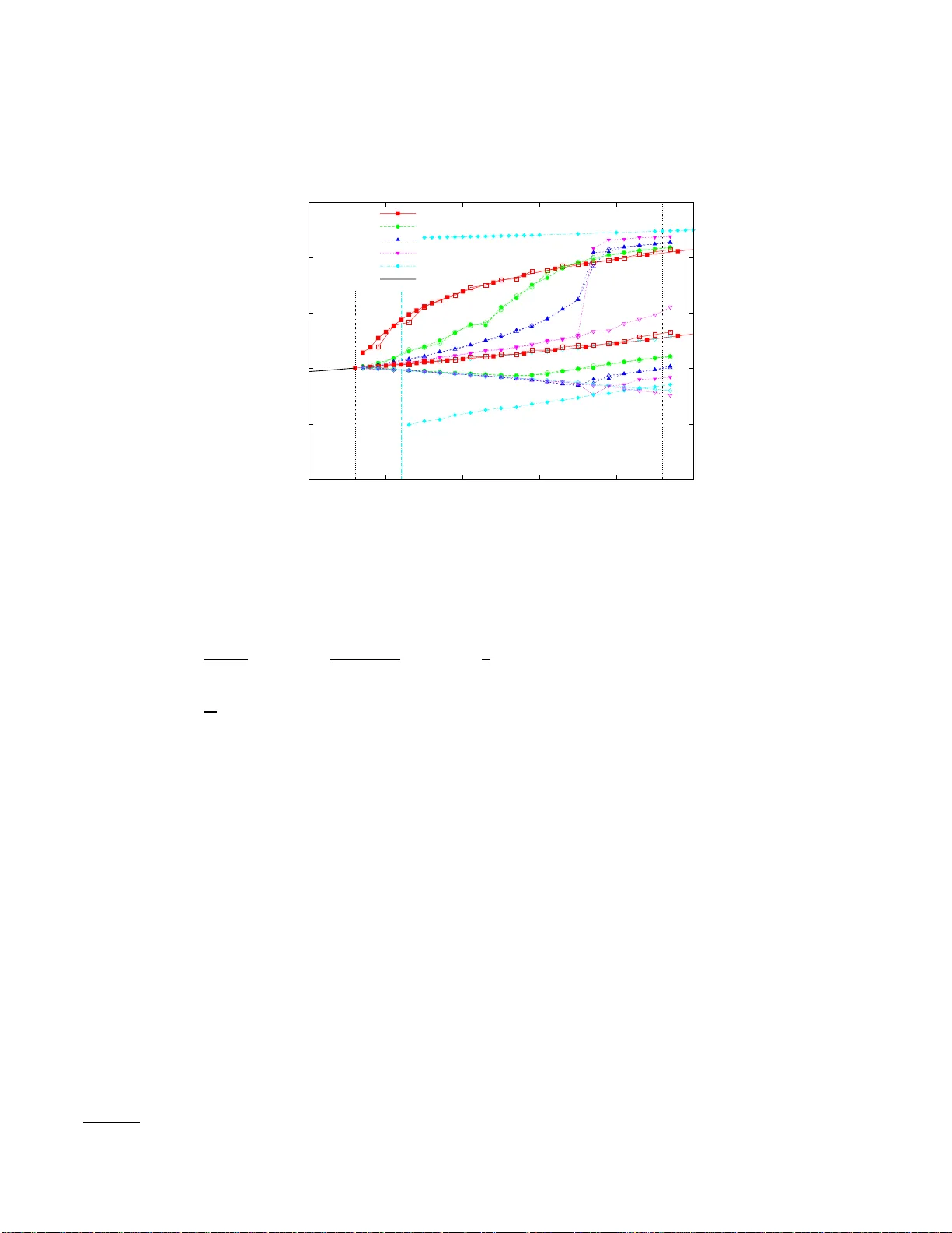
Clusters of solutions a nd replica symmetry breaking in random k -satisﬁabilit y Andrea Montanari Depts of Ele ctric al Engine ering and Statistics, Stanfor d University, USA. F ederico Ricci-T ersenghi Dip artimento di Fisic a and INFM-CNR, Universit` a di R oma L a Sapienza, P. A. M or o 2, 00185 R oma, Italy. Guilhem Semerjian LPTENS, Unit ´ e Mixte de R e cher che (UMR 8549) du CNRS e t de l’ENS, asso ci ´ ee ` a l ’UPMC Univ Paris 06, 24 Rue Lhomond, 75231 Paris Ce dex 05, F r anc e. (Dated: May 29, 2018) W e study the set of solutions of random k - satisﬁabilit y form u lae through the cavit y metho d. It is know n that, for an in terv al of the clause-to-v ariables ratio, this decomp oses into an ex p onentia l num b er o f pure states (clusters). W e reﬁne substantially this picture by: ( i ) determining th e precise location of the clustering transition; ( ii ) uncoveri n g a second ‘condensation’ ph ase transition in th e structure of the solution set for k ≥ 4. These results b oth follo w from computing the large deviation rate of the internal entropy of p ure states. F rom a technical point of view our main con tribu tions are a simpliﬁed version of the ca v ity formalism for special v alues of the Pa risi rep lica symmetry breaking parameter m (in particular for m = 1 via a corresp ondence with th e tree reconstruction problem) and new large- k expansions. I. INTRO D UCTION An instance of k -satisﬁability ( k -SA T) consis ts in a Bo olean formula in conjunctive nor mal form whereby each elementary clause is the disjunction of k literals (a Bo olea n v ar iable o r its negation). Solving it amoun ts to determining whether there exists an a s signment of the v ariables such that a t least one literal in eac h clause e v a lua tes to true. The k -SA T problem plays a cen tral role in the theory of co mputatio nal complexit y , b eing the ﬁr st decision problem prov en to b e NP-co mplete [1] (for all k ≥ 3). Its optimization (minimize the num b er of unsa tisﬁed clauses) and enum eration (count the num b er of optimal assig nment s) versions are deﬁned straig ht forwardly a nd are als o har d fro m the computational po int o f view. Random k - s atisﬁability is the ensemble deﬁned by drawing a uniformly random for mula among all the ones in volving M k -clauses ov er N v aria bles. Equiv alently , each o f the M clause s is drawn uniformly ov er the 2 k  N k  po ssible ones, independently from the other s. It was obser ved empirica lly ea rlier o n [2 ] that, by tuning the clause densit y α = M / N , this ensemble could pro duce formulae which w er e hard for known algorithms. Hardness was argued to b e related to a sha rp thr eshold in the satisﬁability proba bilit y , emer ging as N → ∞ with α ﬁxe d. More precisely , it is b elieved that there exists a constant α s ( k ) such that random formulae are with high probability 1 satisﬁable if α < α s ( k ) and unsatisﬁable if α > α s ( k ). The existence of a sharp threshold was proven in [3], with, how ever, a critical po int α s ( k , N ) which mig ht not conv erg e when N → ∞ . Despite imp or tant progresses [4–6] the rig orous pro of of the existence and determination of α s ( k ) remains a ma jor op en problem (with the notable exception of k = 2 [7]). The connection b etw ee n thre shold phenomena and phase tr ansitions spurred a considerable amoun t of w ork [8–12] using techniques fr om the theory of mean ﬁeld s pin g lasses [1 3]. The ma in outcomes of this appr oach hav e been: ( i ) A pr ecise conjecture o n the lo cation of the satisﬁa bility threshold α s ( k ) [10, 12]; ( ii ) The sugges tion [9, 1 0] fo r k ≥ 3 of another tr ansition at α d ( k ) < α s ( k ) aﬀecting the geometr y of the solutions space; ( iii ) Most strikingly , the prop osal of a new and ex tremely eﬀective messa ge passing algo rithm, Survey Pro pa gation (SP ) [10, 11]. This exploits a detailed statistical picture of the solution space to eﬃcien tly ﬁnd solutions. According to statistical physics studies, in the intermediate regime α ∈ [ α d ( k ) , α s ( k )] solutions tend to gro up themselves in clusters that ar e somehow disconnected. As α increases , the num b er of these clusters decr eases. The satisﬁability trans ition is thus due to the v anishing of the num b er of clusters, which still contain a large n umber of solutions just b efor e α s ( k ). The phase tr ansition at α d ( k ) has b een referred to as “clus tering phase transition” 1 Here and b elow ‘with high probability’ (w.h.p.) means with pr obability con verging to 1 as N → ∞ . 2 or “dynamic pha se transition” depending on the fea ture emphasiz e d. Its nature a nd lo cation, as well as a r eﬁned description of the regime α ∈ [ α d ( k ) , α s ( k )] will be the ma in to pic of this paper. Mo re precisely: ( i ) W e will a rgue that previous determinations o f α d ( k ) [10–12] hav e to b e c orrected when ﬂuctuations o f the cluster sizes are tak en into accoun t; ( ii ) W e will unco ver (for k ≥ 4 ) a new ‘condens a tion’ phase tra nsition a t α c ( k ) ∈ [ α d ( k ) , α s ( k )]. F or α ∈ [ α d ( k ) , α c ( k )] the relev ant clusters ar e exp onentially n umer ous. F or α ∈ [ α c ( k ) , α s ( k )] most o f the so lutions are con ta ined in a n umber of clusters that remains bo unded as N → ∞ . The pap er is org anized as follows. In Section I I we recall so me genera l fea tures of mean-ﬁeld disor dered mo dels, emphasizing the notions of dynamical transitions and replica symmetry breaking. In Section I I I we deﬁne more precisely the ensemble of random formulas studied and describ e the replica sy mmetr ic (RS) and one step of replica symmetry brea k ing (1RSB) approach to this mo del. W e then a pply the progr am of Section I I to the random k - satisﬁability problem and pr esent our main results in Section IV. F or the sake of cla rity some technicalities of the 1RSB trea tmen t are presen ted shortly a fterward, se e Section V. T o complemen t these results, whic h are partly bas ed on a n umerical resolution of in tegra l eq uations, we present in Section VI an asymptotic expansion in the lar ge k limit which gives further cre dit to our theses. W e draw our conclusions in Sec. VI I. T echnical details are deferred to three app endices. A short accoun t of our results has b een published in [14], and a detailed analysis of the related q - coloring problem in [15]. While the pres ent w ork w a s b eing ﬁnished t wo very interesting pa p e r s conﬁrmed the gener ality of the res ults of [14]. The ﬁrst concerned 3-SA T [16] and the second bi-coloring of random h yp erg r aphs [1 7]. II. MEAN-FIELD DISORDERED SYST E M S The goal of this section is to pr ovide a quick overview o f the cavit y metho d [13, 18]. W e will further prop ose a more precise mathematical formulation of several notions that are cruc ia l in the statistical ph ysics appro ach. A. Statistical m echanics and graphical mode l s Let us start b y cons ide r ing a g eneral model deﬁned by: (1) A factor g raph [19], i.e. a bipartite graph G = ( V , F , E ). Here V , | V | = N , ar e ‘v ariable no des’ cor resp onding to v ar ia bles, F , | F | = M , are ‘function (or factor) no des’ describing interactions among these v ariables , and E are edges b e t ween v ariables and factors. Given i ∈ V (resp. a ∈ F ), we sha ll denote by ∂ i = { a ∈ F : ( ia ) ∈ E } (resp. ∂ a = { i ∈ V : ( ia ) ∈ E } ) its neighbor ho o d. F urther, given i, j ∈ V , we let d ( i, j ) b e their gra ph theoretic distance (the minimal n umber of factor no des encountered on a path b etw een i and j ). (2) A space of conﬁgur a tions X V , with X a ﬁnite alphab et, (a conﬁgura tion will b e deno ted in the following as σ = ( σ 1 , . . . , σ N ) ∈ X V ). F or any set A ⊆ V , w e let σ A = { σ i : i ∈ A } . (3) A set of non negative weights { w a : a ∈ F } , w a : X ∂ a → R + , σ ∂ a 7→ w a ( σ ∂ a ). In the ca s e of c onstr aint satisfaction pr oblems , these are often taken to b e indica tor functions (more details o n this particular ca se will b e given in Sec. II D). Given these ingr edients, a measure ov er X V is deﬁned as µ N ( σ ) = 1 Z N w N ( σ ) , w N ( σ ) = Y a ∈ F w a ( σ ∂ a ) . (1) This is well deﬁned only if there exists at leas t o ne conﬁgura tion σ ∗ that makes all the weights strictly po sitive, namely w a ( σ ∗ ∂ a ) > 0 for each a . W e will assume this to be the ca se througho ut the pap er (i.e. we fo cus on the ‘satisﬁable’ phas e). F ur ther, it will b e understo o d that we consider seq uences of graphs (a nd weigh ts) of diverging size N (although we sha ll often drop the subscript N ). An imp ortant role is play e d by the lar ge- N b ehavior of the partition function Z N . This is descr ibed by the 3 free-entrop y density 2 , φ = lim N →∞ 1 N log Z N , Z N = X σ w N ( σ ) . (2) B. Pure s tates and replica symmetry breaking The r eplica/cavity metho d allows to compute a hiera rch y of approximations to φ . This is thought to yield the exact v alue o f φ itself in ‘mean ﬁeld’ models . The hier arch y is or dered accor ding to the so -called nu mber of steps of replica symmetry break ing (RSB). At each level the calculation is based on some h yp otheses on the t ypical structure of µ , a pivotal role b e ing played by the notio n o f pure st ate . Since this co ncept is only intuitiv ely deﬁned in the ph ysics literatur e, we propo se here t wo mathematically precis e deﬁnitions. In b oth c a ses a pure state is a (sequence of ) pro bability meas ures ρ N on X N . • Deﬁnition of pure states through correlation deca y W e deﬁne the correlation function of ρ N as C N ( r ) = sup A,B : d ( A,B ) ≥ r X σ A ,σ B | ρ N ( σ A , σ B ) − ρ N ( σ A ) ρ N ( σ B ) | , (3) where the sup is taken over all subset of v ar iable no des A, B ⊆ V such that the dista nc e be tween any pair o f no des ( i, j ) ∈ A × B is grea ter than r . Then ρ N is a pure state if this cor relation function dec ays at lar ge r . T echnically , w e let C ∞ ( r ) = lim sup N →∞ C N ( r ), a nd require C ∞ ( r ) → 0 as r → ∞ . • Deﬁnition of pure states through conductance W e let the ( ǫ, δ )-co nductance of ρ N be F N ( ǫ, δ ) = inf A⊂X N  ρ N ( ∂ ǫ A ) ρ N ( A )(1 − ρ N ( A )) : δ ≤ ρ N ( A ) ≤ 1 − δ  . (4) Here the inf is taken ov er all subsets of the conﬁg uration space. F urther, letting D denote the Hamming distance in X N , we deﬁned the b o undary of A as ∂ ǫ A = { σ ∈ X N \ A | D ( σ , A ) ≤ N ǫ } . With thes e deﬁnitions ρ N is pure if its conducta nc e is b ounded b elow by an inv erse po lynomial in N for all ǫ and δ (while non-pure states hav e a conductance whic h typically deca ys exp onentially with N ). These tw o deﬁnitions mimic the well-known ones on Z d in terms of tail triviality a nd extr e mality [20]. F urther, the second one is clear ly related to the b ehavior of local Monte Carlo Marko v chain dynamics. A small conductance amounts to a b ottleneck in the distribution and hence to a large rela x ation time. While we e x pe ct them to b e equiv alent for a lar ge family of mo dels, proving this is a lar gely o pe n pr oblem. Moreov er w e should emphasize that the heuristic cavit y method followed in this pap er never explicitly us e s either of these deﬁnitions. The h yp otheses implicit in the cavity metho d can b e expres sed in terms of the pur e states de c omp osition of µ . This is a partition o f the conﬁg uration spac e (dep endent on the g raph and w eig hts) suc h that the measure µ constrained to each element of this par tition is a pure state. More precisely , let us call {A γ } γ a partition of X N , and deﬁne Z γ = X σ ∈A γ w ( σ ) , W γ = Z γ Z , µ γ ( σ ) = 1 Z γ w ( σ ) I ( σ ∈ A γ ) . (5) Clearly µ can b e written a s the c onv ex combination of the µ γ with co e ﬃcie nt s W γ . This deﬁnes a pure state decomp osition if: ( i ) each of the µ γ is a pure state in the sense given ab ove, ( ii ) this is the ‘ﬁnest’ such partition, in the sense that the µ γ are no longer pure if an y subset of them is replaced b y their union. Statistical ph ysics calcula tio ns sugg est that a wide class of mean ﬁeld mode ls is describ ed by one of the following ‘universal b ehaviors’. The terminolog y used here is inherited from the literature on mean ﬁeld spin glasses [21, 22]. 2 One usually assumes that the l imit exists. If the mo del i s disordered, almost sure l imit can b e used, or, equiv alen tly , log Z N is replaced b y its exp ectation. 4 RS Most of the measure is co ntained in a single element of the partition, namely W max = ma x γ W γ → 1 as N → ∞ ( r eplic a symmet ric ). d1RSB Most of the measure is ca rried by N . = e N Σ ∗ pure states 3 , each one with a w eight W γ . = e − N Σ ∗ ( dynamic al one-step r eplic a symmetry br e aking ). 1RSB The meas ure condensates on a sub exp onential n um be r of pur e states, namely , if W [ γ ] is the weight of the γ -th largest state, then lim n →∞ lim N →∞ P n γ =1 W [ γ ] = 1 ( one step re plic a symmet ry br e aking ). The reader will notice that this list do es not include full replica symmetry breaking phas es, in which pure states are organiz e d according to an ultra metric s tr ucture. While this b ehavior is as gener ic as the previo us ones, our understanding of it in sparse graph models is still rather po o r. W e are mostly concerned with families of models of the type deﬁned in Eq. (1) indexed b y a con tinuous par ameter α (suc h as the clause densit y in k -SA T). In this setting, the ab ov e be haviors often a ppea r in sequence as listed ab ov e when the sy stem b ecomes mo r e and mo r e constra ine d (e.g . as α is increa sed in k -SA T). The diﬀerent regimes are then se pa rated by phase trans itio ns: the ‘dynamical’ or ‘cluster ing’ phase tra nsition fro m RS to d1RSB (a t α d ) a nd the ‘condensation’ phase transitio n betw een d 1RSB and 1 RSB (a t α c ). The paradigmatic ex ample of such tra nsitions is the fully-connected p -spin model [2 1, 22], where they are encountered up o n lowering the temper ature. Let us stress that th e ab ov e deﬁnitions are insensitiv e to what happ ens in a fraction of the space of co nﬁgurations of v anishing measure. F or instance, we neg lect metastable states whose o verall weigh t is exp onentially small 4 . A conv enient to ol for distinguishing these v arious behaviors is the replicated free-entrop y [23], Φ( m ) = lim N →∞ 1 N E lo g ( X γ Z m γ ) , (6) where m is an arbitrary real num b er (kno wn as P a r isi re plica symmetry breaking parameter) whic h allows to w e ig ht diﬀerently the v a rious pure states ac c ording to their s iz es. Supp ose indeed that the num b er of pure states γ with int e rnal free-entrop y density φ γ = (lo g Z γ ) / N b ehav e at leading or de r as exp { N Σ( φ γ ) } , where Σ( φ ) is known as the complexity (or conﬁgura tional en tropy) o f the states. The sum in (6) can then b e computed by the Laplac e metho d; if one assumes for simplicit y that Σ is p ositive o n an in terv al [ φ − , φ + ], this leads to Φ( m ) = sup φ ∈ [ φ − ,φ + ] [Σ( φ ) + mφ ] . (7) Provided Σ is concave, it can be rec onstructed in a parametric w ay fr o m Φ( m ) b y a Legendre inv ers ion [23 ], Σ( φ int ( m )) = Φ( m ) − m Φ ′ ( m ) , φ int ( m ) = Φ ′ ( m ) , (8) where m is such that the supremum in (7) lies in the interior of [ φ − , φ + ], which deﬁnes a ra nge [ m − , m + ]. Usually Σ v anishes contin uous ly at φ + . As e xplained b elow, when zero ener gy states a re concer ned φ int ( m ) co incides with the internal en tropy of suc h states . Note that a given v alue o f m selects the p oint of the curve Σ( φ ) o f slop e − m ; in particular the v a lue m = 0 corr e sp onds to the maximum of the curv e. The replica /cavit y method at the level of one step of replica s ymmetry breaking allows to compute the r eplicated free-entrop y Φ( m ) under an a ppropriate hypothesis on the organiza tion of pure states . The v arious regimes can b e distinguished through the b ehavior o f this function, namely RS Φ( m ) = mφ ∗ , where φ ∗ is the contribution o f the single do minant pure sta te, Z [1] . = e N φ ∗ . d1RSB Φ( m ) /m a chiev es its minimum for m ∈ [0 , 1] at m = 1 , with Σ ∗ = Φ(1) − Φ ′ (1) > 0. Then the measure µ decomp oses in to a pproximately e N Σ ∗ pure states of in terna l free-ent ropy Φ ′ (1). 1RSB Φ( m ) /m a chiev es its minimum ov er the interv al [0 , 1] at m s ∈ (0 , 1). Then the ordered sequence of w eig ht s W [1] ≥ W [2] ≥ W [3] ≥ · · · keep ﬂuctuating in the thermo dynamic limit, and conv erg e s to a Poisson-Dirichlet pro cess [24] of parameter m s . The int ernal free-entrop y of these states is Φ ′ ( m s ). In all these cases the total free-en tropy density is estimated by minimizing Φ( m ) /m in the interv al [0 , 1]. 3 Here and in the following . = means equality at the leading exponent ial order. 4 In the f ully connected mo dels suc h metasta bl e state s ar e indeed seen as solutions of the Thouless-Anderson-Palmer equations, w ell abov e the dynamical phase transition. 5 C. Ca vity equations W e shall now recall the fundamen ta l equations used within the 1RSB cavity metho d and prop ose a somehow origina l deriv ation. In the following we will b e interested in fa c tor gr aphs that co nv erge lo cally 5 to trees in the ther mo dynamic limit. In conse quence, let us ﬁrst co nsider the cas e of a mo del of type (1) whose under ly ing factor gr aph is a tr e e, and discuss later how the lo ng lo o ps are taken in to acco unt by the cavity metho d. T ree factor graph mo dels are easily solved b y a ‘messa ge passing’ pro cedure [1 9]. One asso ciates to each directed edg e from factor a to v ar iable i (r esp. from i to a ) a “mess age” η a → i (resp. η i → a ). Messag es are probability mea sures on X . On trees , they can b e deﬁned as the marginal law of σ i with resp ect to the mo diﬁed factor graph G a → i (resp. G i → a ) where all factor no des in ∂ i \ a (resp. the factor node a ) hav e been removed. Simple computations yield the follo wing lo cal equations b e t ween messages, η a → i = f a → i ( { η j → a } j ∈ ∂ a \ i ) , f a → i ( { η j → a } )( σ i ) = 1 z a → i ( { η j → a } ) X σ ∂ a \ i w a ( σ ∂ a ) Y j ∈ ∂ a \ i η j → a ( σ j ) , (9) η i → a = f i → a ( { η b → i } b ∈ ∂ i \ a ) , f i → a ( { η b → i } )( σ i ) = 1 z i → a ( { η b → i } ) Y b ∈ ∂ i \ a η b → i ( σ i ) , (10) where the functions z a re ﬁxed by the normaliz a tion of the η ’s. As we cons ide r a tree factor g raph these equations hav e a unique solution, easily determined in a single sw eep of updates from the leaves of the graph tow ards its ins ide. Moreov er the free entrop y of the mo del follows from this solutio n and reads N φ = log Z = − X ( i,a ) log z ia ( η a → i , η i → a ) + X a log z a ( { η i → a } i ∈ ∂ a ) + X i log z i ( { η a → i } a ∈ ∂ i ) . (11) Here the ﬁrst sum runs o ver the undirec ted edges of the factor graph and the z ’s are given by z ia = X σ i η a → i ( σ i ) η i → a ( σ i ) , z a = X σ ∂ a w a ( σ ∂ a ) Y i ∈ ∂ a η i → a ( σ i ) , z i = X σ i Y a ∈ ∂ i η a → i ( σ i ) . (12) This computation is corre ct only on tr e e factor graphs. Nevertheless it is exp ected to yield go o d estimates o f the marginals and free en tropy for a n umber of mo dels on lo cally tree-like gr aphs. The belief pr opagatio n (BP) alg orithm consists in iterating E qs. (9,10) in order to ﬁnd an (appr oximate) ﬁxed p oint. In pa rticular, whenever the RS sce na rio holds, ther e s ho uld b e one approximate solution o f the ab ov e equations that yields the c orrect leading order o f the free ent ropy density in the thermo dynamic limit. In any case, when dealing with random factor graphs , one can alwa y s turn this simple computation int o a probabilistic one, deﬁning a distribution of random messa g es by r eading (9 ,10) in a distributional sense with rando m weight functions and v ariables’ degrees. The RS es timate of the av e rage free ent ropy is then obtained by a veraging the v ar io us terms in (11) with r esp ect to these random messages. This appro ach can be r eﬁned in d1RSB and 1R SB regimes . The BP equations (9,10 ) should be a pproximately v alid if one computes the messages η a → i and η i → a as mar ginal laws of the measure µ γ restricted to a single pure sta te γ . When the num b er of pure states is very la rge, one conside r s a distribution (with r esp ect to the pur e states γ with their weigh ts W γ ) of messages on eac h directed edge o f the factor graph. A simple and suggestive der iv ation of the 1RSB equations go es as follows. Assume that the factor graph is a tree, and cho ose a subset B of the v ariable no des that will act a s a b oundary , for insta nce (but not neces sarily) the leav es of the factor graph. E ach conﬁgura tion σ B of the v ariables in B induces a conditional distribution µ σ B on the re maining v ariables, µ σ B ( τ ) = 1 Z σ B w ( τ ) I ( τ B = σ B ) , (13) where here a nd in the fo llowing I denotes the indicator function of an even t, and the normalizing fa c tor Z σ B is the partition function restricted to the conﬁgurations coinciding with σ B on the boundar y . 5 More precisely , any ﬁnite neighborho o d of a uniformly c hosen random ve rtex con verges to a tree. 6 Since the factor gra ph corresp o nding to µ σ B is still a tree, the corresp onding marginals and par tition function Z σ B can b e co mputed iterating the message passing eq uations (9,10), with an a ppropriate prescription for the messag es η i → a emerging from v ariables i ∈ B , namely η i → a ( τ i ) = δ σ i ,τ i . Let us denote b y η σ B a → i and η σ B i → a the co rresp onding s et of messages, solutions of (9,10) on all edges of the factor graph. F ur ther deﬁne, for m ∈ R , a pro bability meas ure on the bo undary conditions as ˜ µ ( σ B ) = ( Z σ B ) m P σ ′ B ( Z σ ′ B ) m . (14) The ide a is to mimic the pure states of a lar ge, lo o py factor graph mo de l, by the b o undary conﬁgura tions of a tree mo del. Calling P a → i (resp. P i → a ) the distribution of the messa ges η σ B a → i (resp. η σ B i → a ) with resp ect to ˜ µ 6 , a sho rt reasoning reveals that P a → i ( η ) = 1 Z [ { P j → a } , m ] Z Y j ∈ ∂ a \ i d P j → a ( η j → a ) δ ( η − f a → i ( { η j → a } )) z a → i ( { η j → a } ) m , (15) P i → a ( η ) = 1 Z [ { P b → i } , m ] Z Y b ∈ ∂ i \ a d P b → i ( η b → i ) δ ( η − f i → a ( { η b → i } )) z i → a ( { η b → i } ) m , (16) where the functions f and z ar e deﬁned in Eq. (9), (10), and the Z [ · · · ] are nor ma lizing factor s deter mined by the condition R d P a → i ( η ) = R d P i → a ( η ) = 1. E q uations (15), (16) coincide with the s ta ndard 1RSB equatio ns with Parisi parameter m [2 5]. In addition the fre e entrop y density asso ciated to the law ˜ µ , N Φ( m ) ≡ lo g { P σ B ( Z σ B ) m } can b e shown to b e N Φ( m ) = − X ( i,a ) ∈ E log Z ia [ P a → i , P i → a , m ] + X a ∈ F log Z a [ { P i → a } i ∈ ∂ a , m ] + X i ∈ V log Z i [ { P a → i } a ∈ ∂ i , m ] , (17) where the factors Z ··· are fractional momen ts of the ones z ··· deﬁned in Eq. (12), namely Z ia = Z d P a → i ( η a → i )d P i → a ( η i → a ) z m ia , Z a = Z Y i ∈ ∂ a d P i → a ( η i → a ) z m a , Z i = Z Y a ∈ ∂ i d P a → i ( η a → i ) z m i . (18) As in the RS case, one can heuris tically apply (15,1 6) on any graph, even if it is no t a tree. O f particular interest is the limit B → ∅ . E quations (1 5), (16) may hav e t wo behaviors in this limit: ( i ) All the distributions P i → a , P a → i bec ome Dira c deltas in this limit. In this ca s e a ‘far aw ay’ b oundary has small inﬂuence on the system, a nd it is easily seen by compar ing (11) a nd (17) that Φ( m ) = mφ . ( ii ) These distributions remain non-tr ivial in the limit B → ∅ . This case is in terpr eted as a conse q uence of the existence of many pure states. In this situation, ev en a small bo undary inﬂuences the system by selecting one o f s uch states . W e thus in terpret the B = ∅ limit of Φ( m ) as an estimate of the replicated potential (6). In Sec. I I B we emphasized the sp e cial r o le play ed by the v a lue m = 1: the dynamical transition is signaled by the app eara nce of a non-triv ial solution of the 1RSB eq uations with m = 1. This is par ticularly clear in the present deriv ation of the 1RSB equations. Indeed, the distribution ˜ µ of the b oundar y co ndition coincides in this case with the Boltzmann distribution µ . The existence of a non-trivia l solution of the 1RSB equa tions at m = 1 is thus related to a peculia r form of long range co r relations under µ , as ﬁrs t p ointed out in [26]. Such co rrelatio ns can be measur ed through a p oint-to-set correla tion function [27–29]. F or co ncreteness let us g ive an ex pr ession of this c orrela tion in the case of Ising spins . Given a v ar ia ble node i and a set of v ar iable nodes B , we let C ( i, B ) ≡ X σ B µ ( σ B ) X σ i µ ( σ i | σ B ) σ i ! 2 − X σ i µ ( σ i ) σ i ! 2 . (19) The reader will r ecognize the analog y b e t ween this expressio n and the diﬀerence q 1 − q 0 of intra and inter-state ov erla ps [30]. The Bo ltzmann measure has long ra nge po int-to-set cor relations if C ( i, B ) do es not decay to 0 when d ( i, B ) gr ows. Such correlations w ere shown in [31, 32] to imply a div er ging relaxation time. 6 more precisely , wi th r espect to the measure ˜ µ a → i (resp. ˜ µ i → a ) deﬁned sim ilarly f or the factor graph G a → i (resp. G i → a ). 7 D. Application to constraint satisfaction proble ms This short ov er view of the cavit y method did no t rely on any hypothesis on the for m o f the weigh t factors w a in Eq. (1 ). W e now comment brieﬂy on the way this general for malism is applied to co nstraint s atisfaction problems (CSP), in order to cla rify the rela tionship of the present w or k with previous studies. In a CSP the factors a corresp o nd to c onstraints, which can be either sa tisﬁed or not b y the co nﬁguration of their adjacen t v a r iables, σ ∂ a . F or a sa tisﬁable instance o f a CSP one can take w a to b e the indicator function of the ev ent ‘co nstraint a is satisﬁed.’ Then the law deﬁned in (1) is the uniform distr ibutio n over th e solutio ns of the CSP , the pa rtition function counts the nu mber of such solutions and the free entropy r educes to the logarithm o f the num b er of solutions . This “entropic” metho d [33] is the most adequate to the study of the satisﬁa ble phase. This approach is how ever ill-deﬁned for unsatisﬁa ble instanc e s. The us ual way to ha ndle this ca se is to deﬁne a cost function E ( σ ) o n the space o f conﬁgurations , equal to the num b er of unsa tisﬁed constraints under the a ssignment σ . F ollowing the traditiona l notations of statistical mechanics one introduces an inv ers e tempera ture β a nd weighs the conﬁgur ations with w ( σ ) = exp[ − β E ( σ )]. Small tempe r atures (la r ge β ) favor low-energy conﬁguratio ns , in the limit β → ∞ the measure µ concentrates o n the o ptimal conﬁgura tions which maximizes the n um be r of satisﬁed constraints. Let us detail this appr oach which was o riginally follow ed in [10, 1 2, 34]. At the 1 RSB level the pure states are c haracter ized by th eir energy density e and their entrop y densit y s , with the free en tropy de ns it y given by φ = s − β e . Deﬁning the complex it y Σ( s, e ) ac c ording to the n um be r of pure s tates with these tw o characteristics, Eq. (7) beco mes Φ( β , m ) = s up s,e [Σ( s, e ) + m ( s − β e )] . (20) If o ne takes now the limit β → ∞ and assume e > 0, the entropic term b ecomes ir relev ant; to obtain a ﬁnite result one has to take at the sa me time m → 0 such that the pro duct β m , usually denoted y , r emains ﬁnite. One thus obtains Φ e ( y ) = sup e [Σ e ( e ) − y e ] , Σ e ( e ) ≡ sup s Σ( s, e ) . (21) In the unsatisﬁable phase, the ‘energetic’ cavit y approach allows to characterize the minimal energy of the pr oblem. In the ca se of satisﬁable pr oblems, o ne has to p er form a s econd limit y → ∞ (after β → ∞ ) to concentrate o n the pure sta tes with e = 0. It follows that the complexity thus computed is sup s Σ( s, e = 0), i.e. the maximum of the en tropic complexity . In other words the pr o cedure y → ∞ after β → ∞ is equiv alent to p er form the entropic computation with a Parisi parameter m = 0, i.e. to weigh all the pure states in a s ame wa y , ir r esp ectively of their sizes. This is not a pr oblem for the deter mination of the sa tis ﬁa bility th reshold α s , which corresp onds to the disapp ea ring of all zero-energ y pure sta tes, hence to the v a nishing of the maximal complexit y Σ( m = 0). Howev er the v alue of α d in [1 0, 12] corresp onds to the app eara nce of a solution of the 1RSB equations with m = 0 , a nd no t with m = 1 whic h we arg ued to be the relev ant v alue for the deﬁnition of α d . In the rest of the pap e r we shall follow the entropic cavit y metho d, i.e. w e take (1 ) to b e the uniform measure ov er the solutions of the CSP under study and keep a ﬁnite v a lue for the Parisi para meter m . Befor e entering the details of this approach o n the example of r andom k -satisﬁability , let us mention that the existence of expo nentially nu merous pure s tates (ca lled clusters in this context) for so me v alues o f α and k , has b een proved in [35, 36]. An int r insic limita tio n of these works was that cluster s were deﬁned by muc h stricter conditions than the one ex po sed ab ov e (which th us implied limita tio ns on α , k ). The conseq uences of the existence of a distribution of cluster ’s sizes hav e also been inv es tigated in a toy model in [37]. W e s hould also emphasize that for the simpler CSP known as X O RSA T [38, 39], a pr e c ise characteriza tio n of the clusters has been a chieved through rigorous methods. A go o d part of the phenomena s tudied in the present pap er is how ever a bsent of this simpler mo del. In par ticular all clusters of XORSA T ha ve the same size because of the linear structure of the constraints. II I. THE CA VITY MET HOD APPLIED T O THE RANDOM k -SA T PR OBLEM A. Some deﬁnitions In the application of the forma lism to k - satisﬁability , w e use σ i ∈ X = {− 1 , +1 } to enco de the Bo olea n v ar iables. A co nstraint a on k v aria bles σ ∂ a is satisﬁed b y all the 2 k conﬁguratio ns except one, let us call it J a = { J a i : i ∈ ∂ a } , 8 j ′ a i b c j j ′′ FIG. 1: An example of the factor graph representation of a satisﬁability form ula for k = 3. The va lues J a i are enco ded by draw ing a solid ( resp. dashed) edge b etw een clause a and vari able i if σ i = +1 (resp. − 1) satisﬁes clause a . The distances b etw een some of t h e va riable no des are d i,j = d i,j ′ = d i,j ′′ = 1 and d j,j ′ = 2. The neigh b orhoo ds are for instance ∂ i = { a, b, c } , ∂ a = { i, j, j ′′ } , ∂ + i = { a } , ∂ − i = { b, c } , ∂ + i ( a ) = ∅ , ∂ − i ( a ) = { b, c } , ∂ + i ( b ) = { c } , ∂ − i ( b ) = { a } . in which all the literals of the cla use a r e false. The weight factor s are thus deﬁned as w a ( σ ∂ a ) = I ( σ ∂ a 6 = J a ), the indicator function of the ev ent “clause a is s atisﬁed.” A for mula is repres e nted as a factor gr aph (cf. Fig. 1) whose edges are lab eled by J a i . This s ug gests to reﬁne the deﬁnition o f the neighborho o ds . Given a v a riable no de i , ∂ + i (res p. ∂ − i ) will denote the set of clauses which a re satisﬁed b y σ i = + 1 (res p. σ i = − 1). F ur ther, given a clause a ∈ ∂ i w e call ∂ + i ( a ) (resp. ∂ − i ( a )) the set of cla uses in ∂ i \ a which a re satisﬁed b y the same (resp. opp osite) v alue of σ i as is a . F or k -SA T formulas the general RS cavity equa tions (9), (10) can be written in a pretty ex plic it for m. As the v ariables take only tw o v alues the cavit y pr obability mes s ages η a → i and η i → a can b e parametr ized by a single real nu mber, that w e s ha ll call respectively u a → i and h i → a and deﬁne by η a → i ( σ i ) = 1 − J a i σ i tanh u a → i 2 , η i → a ( σ i ) = 1 − J a i σ i tanh h i → a 2 . (22) With these conv entions Eqs . (9), (10) tak e the form u a → i = f ( { h j → a } j ∈ ∂ a \ i ) , f ( h 1 , . . . , h k − 1 ) = − 1 2 log 1 − k − 1 Y i =1 1 − tanh h i 2 ! , (23) h i → a = X b ∈ ∂ + i ( a ) u b → i − X b ∈ ∂ − i ( a ) u b → i . (24) W e a re interested in the regime wher e the num b er M of uniformly c hosen clauses and the num b er of v a riables N bo th diverge at ﬁxed r a tio α = M / N . The rando m factor graphs thus genera ted enjoy prop erties r eminiscent o f the Erd¨ os-R ´ enyi random gr aphs G ( N , M ) [4 0, 41]. In particular, for a uniformly r andom v ariable no de i , the num b er of clauses in ∂ + i and ∂ − i con verges to tw o i.i.d Poisson r andom v ar iables of mean αk / 2. The same statement is tr ue for ∂ + i ( a ) a nd ∂ − i ( a ) w hen ( i, a ) is an uniformly c hosen edge of the factor g raph. The degree distribution is a v ery loca l description of a graph, lo o king at o ne node or edge only . It is ho wever easy to sho w tha t an y b ounded neighborho o d of a uniformly random node i conv e r ges to a rando m (Galton-W atso n) tree with the same degree distr ibution [41]. B. The RS description of the random formulae ensemble The replica-s ymmetric trea tment of the random k -SA T pr o blem w a s ﬁrst w o rked out using the replica formalis m in [8]. In the cavit y fo rmulation one interprets the BP equations (9,1 0 ,23,24 ) in a proba bilistic wa y . More precis ely , we introduce the dis tributions of u a → i , h i → a (ov er the c hoice of the r andom formula) and denote them as P (0) ( h ) and Q (0) ( u ). These distributions sa tisfy the distributional equations: u d = f ( h 1 , . . . , h k − 1 ) , h d = l + X i =1 u + i − l − X i =1 u − i . (25) 9 In these expres sions h, { h i } (resp. u, { u ± i } ) are indep endent copies of the random v ariable of distribution P (0) ( h ) (resp. Q (0) ( u )), the function f is deﬁned in Eq. (23) and l ± are two independent Poisson rando m v ariables of mean αk / 2. The symbol d = denotes iden tity in distribution 7 . The RS prediction for the en tro py r eads φ (0) = − αk E log z 1 ( u, h ) + α E log z 2 ( h 1 , . . . , h k ) + E log z 3 ( u + 1 , . . . , u + l + , u − 1 , . . . , u − l − ) , (26) where the exp ec ta tions are over i.i.d. copies of the r andom v ar iables u and h , and l ± are as a b ov e. T he v ario us ent ropy shifts are obtained by rewriting th e z ’s in Eq. (12) in terms o f u and h , z 1 ( u, h ) = 1 + tanh h tanh u , (27) z 2 ( h 1 , . . . , h k ) = 1 − k Y i =1 1 − tanh h i 2 , (28) z 3 ( u + 1 , . . . , u + l + , u − 1 , . . . , u − l − ) = l + Y i =1 (1 + tanh u + i ) l − Y i =1 (1 − tanh u − i ) + l + Y i =1 (1 − tanh u + i ) l − Y i =1 (1 + tanh u − i ) . (2 9 ) Similarly the RS ov erlap can be computed as q 0 = E [tanh 2 h ] . (30) Several equiv alent e x pressions of the RS entrop y can be found in the literature; the choice we made in (26) has the adv antage of b eing v ar iational. By this we mean that the statio narity conditions of the function φ (0) [ P , Q , α ] with resp ect to P and Q are nothing but the self-consistency equations (25). Note also that the rigorous results of [42, 43] imply that 8 the entrop y dens it y φ is upp er-b o unded by the RS φ (0) for any trial distribution P , a s long as Q is linked to P by the ﬁr st equa tio n in (25), for a reg ula rized version of the mo del at ﬁnite temp erature. Mo reov er the RS description was pr ov en to be v alid for small v a lues of α in [44]. The numerical reso lution of the equation on the order par a meter is r elatively easy . The distributio ns P (0) and Q (0) can indeed b e repr esented by samples (or po pulations) of a large num b er N o f representativ es, { h i } N i =1 and { u i } N i =1 . The ﬁxed point condition stated in (25) is looked for by an iterativ e population dynamics algo r ithm [25, 4 1, 45]. W e turn now to the cavity formalism at the 1 RSB le vel, which assumes the organiza tion of pure states describ ed in Section II B. C. The 1RSB description of the random formulae ensemble As in the RS case, when the underlying formula is ra ndom, the messa ges P i → a , P a → i along a uniformly r andom edge beco me random v ar iables, whose distributions are denoted as P (1) [ P ], Q (1) [ Q ]. These distributions satisfy a couple of distributional equations, that are the probabilistic v er sion of Eqs. (15,16), Q ( • ) d = 1 Z 4 [ P 1 , . . . , P k − 1 ] Z k − 1 Y i =1 d P i ( h i ) δ ( • − f ( h 1 , . . . , h k − 1 )) z 4 ( h 1 , . . . , h k − 1 ) m , (31) P ( • ) d = 1 Z 3 [ { Q + i } , { Q − i } ] Z l + Y i =1 d Q + i ( u + i ) l − Y i =1 d Q − i ( u − i ) δ   • − l + X i =1 u + i + l − X i =1 u − i   z 3 ( { u + i } l + i =1 , { u − i } l − i =1 ) m , (3 2) 7 More explicitly , giv en tw o random v ari ables X and Y we write X d = Y if the distributions of X and Y coincide. F or instance, if X, X 1 , X 2 are ii d standard normal random v ariables, X d = ( X 1 + X 2 ) / √ 2 8 In [42, 43] this claim is made for k even . How ever the proof holds verbatim for k o dd as well. T o th e best of our kno wledge, this was observ ed ﬁrst by Eli tza Manev a in 2005. 10 where the P ’s (resp. Q ’s) are i.i.d. from P (1) (resp. Q (1) ) and l ± hav e the ab ov e stated Poissonian distr ibution. The ent ropy shift z 3 used in Eq. (32) w as deﬁned in Eq. (29), while z 4 is given by z 4 ( h 1 , . . . , h k − 1 ) = 2 − k − 1 Y i =1 1 − tanh h i 2 = 1 + e − 2 f ( h 1 ,...,h k − 1 ) . (33) Finally , the 1RSB po ten tial is obtained b y taking the exp ectation of Eq. (17). One gets Φ( m ) = − αk E log Z 1 [ Q, P ] + α E log Z 2 [ P 1 , . . . , P k ] + E log Z 3 [ Q + 1 , . . . , Q + l + , Q − 1 , . . . , Q − l − ] , (34) where the factors Z i are weigh ted av erag es of the corr esp onding entropy shifts, Z 1 [ Q, P ] = Z d P ( h )d Q ( u ) z 1 ( u, h ) m , (35) Z 2 [ P 1 , . . . , P k ] = Z k Y i =1 d P i ( h i ) z 2 ( h 1 , . . . , h k ) m , (36) Z 3 [ Q + 1 , . . . , Q + l + , Q − 1 , . . . , Q − l − ] = Z l + Y i =1 d Q + i ( u + i ) l − Y i =1 d Q − i ( u − i ) z 3 ( u + 1 , . . . , u + l + , u − 1 , . . . , u − l − ) m . (37) The int er and in tra- state ov erlaps are g iven, res pe ctively , by q 0 = E "  Z d P ( h ) tanh h  2 # , q 1 = E  Z d P ( h ) tanh 2 h  . (38) The v ar iational property discussed at the RS lev el still applies to the 1RSB p o tent ial. This is o f pa rticular in terest for the computatio n o f the internal ent ropy of the states, g iven by a deriv a tive with resp ect to m . This deriv ation ca n be a pplied to the explicit dependence only , and yields φ int ( m ) = − αk E  R d P ( h )d Q ( u ) z 1 ( u, h ) m log z 1 ( u, h ) Z 1 ( Q, P )  + α E " R Q k i =1 d P i ( h i ) z 2 ( { h i } k i =1 ) m log z 2 ( { h i } k i =1 ) Z 2 [ { P i } k i =1 ] # + E " R Q l + i =1 d Q + i ( u + i ) Q l − i =1 d Q − i ( u − i ) z 3 ( { u + i } l + i =1 , { u − i } l − i =1 ) m log z 3 ( { u + i } l + i =1 , { u − i } l − i =1 ) Z 3 [ { Q + i } l + i =1 , { Q − i } l − i =1 ] # . (39) The rigorous results of [42, 43] also imply φ ≤ Φ( m ) /m for an y v a lue of m in (0 , 1), and an y trial order parameter P (with Q deﬁned b y Eq. (31)). The numerical reso lution of the 1RSB equations (31,32 ) is in general muc h harder than the one of their RS counterparts (compare with Eq. (25)). The po pulation dynamics a lgorithm r epresents P (1) by a sample of distributions { P i } N i =1 , which themselv es hav e to b e enco ded, for each i , by a ﬁnite set o f cavit y ﬁelds { h i,j } N ′ j =1 . This drastica lly limits the sizes N and N ′ , and hence the precisio n o f the n umerical results. Mor eov er generating one element, s ay Q i , from k − 1 P i ’s is by itself a non trivial task. The v ar ious ﬁelds representing Q i are weighted in a non uniform wa y because o f the factor z m 4 in Eq. (31), whic h forc e s the us e of delicate resampling procedur es. These equations ca n be gr eatly s impliﬁed analytically for t wo par ticular v alue s of m , namely 0 a nd 1. F or the sake o f readability w e p ostp one the discussio n of these imp o rtant simpliﬁcations un til Sectio n V, and pro ceed in the next s ection with the presentation and the in terpretation of the r esults o btained either at arbitrary m with the full nu merical pro cedure (whose implement ation details are exp osed in Appendix A) or in m = 0 , 1 with the simpliﬁed, more precise ones. IV. TRANSITIONS IN THE SA TISFIABLE REGIME OF RANDOM k -SA T A. The dynami cal, condensation and s atisﬁability tr ansitions for k ≥ 4 Let us b egin our discussio n o f the satisﬁable regime of random k -SA T b y studying the case k = 4, the v alues k ≥ 4 having the same qualitativ e behavior. On the o ther hand, the phenomenology of 3-SA T is diﬀer e nt and w e rep ort on 11 ℓ C ℓ 150 120 90 60 30 0 0.6 0.4 0.2 0 FIG. 2: The p oint-to-set correlation function for k = 4, from left to rig ht α = 9 . 30, α = 9 . 33, α = 9 . 35 and α = 9 . 40 -0.02 0 0.02 0.04 0.06 0.08 8 8.5 9 9.5 10 10.5 α Σ (m = 0) Σ (m = 1) φ (m = 0) φ (m = 1) φ RS φ (m = m s ) α d α c α s FIG. 3: The complexity Σ and the in ternal en tropy φ int for t he v alues m = 0 , 1, and m = m s in the 1RSB regime, for k = 4. it in Sec. IV D. F ollowing the progr am of Sec. II we ﬁrst hav e to determine the v alue α d for the app earanc e of a non-tr ivial solution of the 1RSB equa tions with m = 1 . T o this aim we compute the p oint-to-set corre lation function C ℓ , that is the av era ge of the corr e lation function (19) b etw ee n a ra ndomly chosen v aria ble i and the set B of v aria bles at distance ℓ from it. The plo ts of Fig. 2 show that for α ≤ α d ≈ 9 . 38 this cor relation v anishes at large distance, while for larger v a lue s of α a strictly positive long range cor relation sets in discon tinuously . T o distinguish b etw een the d1RSB and 1RSB r egime we then compute the complexity Σ( m = 1). As demo nstrated in Fig. 3 this is strictly pos itive at α d , then decrea ses contin uously until it v a nishes a t α c ≈ 9 . 547. Finally the satisﬁability transition α s is found from the criterio n of v anishing of Σ( m = 0), i.e. the maximum of the entropic complexity curve (see Fig. 3 ): the v alue α s ≈ 9 . 93 1 is in ag reement with [12] and we sha ll sho w in Sec. V B that this is indeed the s ame calculation. T o summarize , we ﬁnd the thr e e regimes RS , d1 RSB , 1RSB describ ed in Sec. I I B o ccurring in this or der, for the v alues of α in [0 , α d ], [ α d , α c ] a nd [ α c , α s ]. W e exp ect this pattern of tra nsitions to b e the sa me for a ll k ≥ 4. This is supp or ted by our numerical in vestigations for k = 4 , 5 , 6 (see T ab. I for a summary of the numerical v alues of the thresholds), and by the larg e- k expa nsions present ed in Sec. VI. The ent ropy densit y (see Fig. 3) is given b y the RS formula both in the RS and d1RSB regimes. In the latter case it has to be understo o d as the sum of the co mplexity Σ( m = 1) and of the internal ent ropy of the asso ciated sta tes, φ int ( m = 1 ). O n the contrary for α ∈ [ α c , α s ] it is necessary to compute the whole function Σ( φ ) by v ary ing m . The ent ropy density coincides with the one of dominan t clusters, and is given by the p oint where Σ( φ ) v anishes. 12 k α d α c α s [12] α f 3 3.86 3.86 4.267 * 4 9.38 9.547 9.9 31 9.88 5 19.16 20.80 21.117 * 6 36.53 43.08 43.37 39.87 [46] T ABLE I: Nu merical val ues of the v arious cri tical thresholds. F or k = 3 w e ha ve f ormally α c = α d , see the text for details on the nature of the d iﬀerence b etw een k = 3 and k ≥ 4. -0.02 -0.01 0 0.01 0.02 0.03 0.04 0 0.01 0.02 0.03 0.04 0.05 0.06 0.07 0.08 0.09 Σ(φ) φ α = 9.3 α = 9.45 α = 9.6 α = 9.7 α = 9.8 α = 9.9 FIG. 4: The complexity Σ( φ ) for k = 4 and sev eral v alues of α : from top to bottom α = 9 . 3, 9 . 45, 9 . 6, 9 . 7, 9 . 8 and 9 . 9. B. The entropic complex i ty cur ves The curves Σ( φ ) a re shown in Fig. 4 for several v alues of α . T he symbols ar e obtained in a parametric wa y , by solving the 1 RSB equations for v arious v alues o f m and plo tting the p oint ( φ int ( m ) , Σ( m )). The lines in Fig. 4 ar e nu merical in terp o la tions, obtained b y ﬁtting not directly Σ( φ ), but ins tead the data for Φ( m ) with a generic smoo th function 9 and then analy tica lly der iving the ﬁtting function to obtain the curves in Fig. 4. The a greement of this ﬁtting pro cedure with the parametric plot is excellen t. The three regimes are clearly illustrated on this ﬁgure: • F or α < α d a p ortion of the curve Σ( φ ) can exist (for instance there is a solution of the 1RSB equation with m = 0 for α ≥ 8 . 297 [1 2]), yet it has no p oint of s lop e − m = − 1. The contribution o f these clus ters is negligible compared to the dominan t RS cluster. • F or α ∈ [ α d , α c ] (see e.g. α = 9 . 45 data in Fig. 4 ) the complexity Σ( m = 1) ex ists and is p os itive (it is marked by a black c ircle in the ﬁgure). • F or α ∈ [ α c , α s ] (see e.g. α = 9 . 6 , 9 . 7 , 9 . 8 , 9 . 9 in Fig . 4) the complexity Σ( m = 1) is negative and th us the Σ( φ ) curve v anishes a t φ ( m s ) (marked with a black squa re), where the slope (in a bs olute v alue) is smaller tha n 1 a nd equals m s ( α ). The measure is dominated b y a subexp onential n umber of clus ters of en tropy φ ( m s ), sho wn as a function of α in Fig. 3. 9 W e ha ve tried diﬀerent ﬁtting functions and all provide equiv alen t and ve ry goo d r esults thanks to the smo othness of Φ( m ). 13 0 0.2 0.4 0.6 0.8 1 9.4 9.5 9.6 9.7 9.8 9.9 10 m α m s m f FIG. 5: The v alue of the P arisi parameter m s in t he thermo dynamically relev ant pure states of the 1RSB regime in random 4-SA T, an d the freezing transition m f . The v alue thus estimated of th e P arisi par a meter m s ( α ) in the 1RSB regime is plotted in Fig. 5 (it is iden tical to 1 in the d1RSB region). The curve close to the m s data is not a ﬁt, but instead an explicit approximate expre s sion for m s ( α ) which b ecomes exact in the large k limit (see Sec. VI for details). Indeed Eq. (81) (v alid to leading o rder at large k ) can be equiv alently rewritten as α s − α α s − α c = 1 − 2 m (1 − m log 2) 2 log 2 − 1 , (40) and this gives a n expressio n for m s ( α ) once v alues of α c and α s determined numerically for k = 4 ar e plugged in to Eq. (40 ). Note that the solution to Eq . (40) is s uch that ( i ) m s ( α c ) = 1, ( ii ) m s ( α s ) = 0 and ( iii ) m s v anishes as a square r o ot at α s . The ﬁnite k cor rections to the ex pression (40) see m a lready sma ll for k = 4, as can b e infer red from the go o d agr eement with the numerical data displa yed in Fig. 5. This fact w a s also noticed for the coloring problem in [15]. Once we co mpute the optimal v a lue m s for ea ch v alue of α , we can plot in Fig. 6 the ov er lap q 0 and q 1 of the dominating clusters as a function of α . Notice that the int er-state ov e r lap q 0 is an increasing function of α for any ﬁxed v alue of m , but becomes a decreasing function of α betw e en α c and α s where w e take m = m s ( α ). W e did not attempt a complete determination of the p ortion of the plane ( α, m ) where non-triv ial so lutions of the 1RSB equations c an be fo und. F rom our numerical inv estigatio ns it seems that solutions with smaller v a lues of m app ear at s maller v alues of α , i.e. the threshold α d ( m ) is a n increa sing function in the range of par ameters we considered. In particula r , solutions with negative m app ear at rather small v alues of α . The limit o f very lar ge neg ative v alues of m is how ever diﬃcult to study n umer ically , a nd mo re work could be done on this issue; the c o rresp o nding pure states ar e tiny because their v a riables are ov er constrained, whic h plagues the numerical resolution of the 1RSB equations. C. On the presence of frozen v ariables in cl usters of solutions Another c hara cterization of the clusters of s o lutions, besides their internal entrop y and self-ov erla p, is th e presence or not of froze n v aria bles, that is v ar ia bles that take the s a me v a lue in all the so lutions of the cluster . In technical terms this corr esp onds to a non-v anishing weight on ±∞ in the 1RSB cavit y ﬁeld distributions P ( h ) (see Eq. (59) below). Our data s how that, given a v alue of α , there exists a threshold m f ( α ) such that c lus ters descr ibe d by m < m f do contain frozen v ariables , while those with m > m f do not. This is consistent with the intuit ion: the freezing of v ariables is c orrela ted with a sma ller v alue of the int ernal ent ropy , hence of m . Numerical estimates fo r the line m f ( α ) 14 0 0.2 0.4 0.6 0.8 1 9 9.2 9.4 9.6 9.8 10 α q 1 (m=0) q 1 (m=m s ) q 1 (m=1) q 0 (m=1) q 0 (m=m s ) q 0 (m=0) q RS α d α c α s FIG. 6: I ntra and inter-state ov erlaps for k = 4. are plotted in Fig. 5 for k = 4. The larg e error bars ar e due to the fact that we hav e ch eck ed the presence of frozen v ariables only at m v alues which are multiples o f 0 . 1 (and no in terp olation can b e done in b etw een, since the pro pe rty is just true or false). The interp olating curve is a ﬁt to the m f ( α ) data w ith the function A ( x − 8 . 297 ) B (for m = 0 the cr itical v alue o f α is α d ( m = 0) ≈ 8 . 297 [12]). The freezing transition α f is deﬁned by the app eara nce of frozen v ariables in dominating clusters, that is m s ( α f ) = m f ( α f ). F rom the crossing of these t wo lines in Fig. 5 we estimated the freezing threshold for k = 4 at α f ≈ 9 . 88 . The fact that the freezing transition o ccurs after the condensa tion one for k = 4 is not g eneric; for k ≥ 6 the threshold m f ( α ) reaches 1 at α f ≤ α c [46], hence in a part of the d1 RSB regime the do mina ting clusters do cont ain frozen v ariables for these v alues of k . Let us how ever emphasize that generally α d < α f , i.e. that in random k -satisﬁability (and also in q -color ing [15]) clustering can o ccur without implying the freezing of v ariable s . This fact has been obscured up to now because the energetic cavity metho d [10, 34] fo cused precisely on the fr action of frozen v ar iables in the m = 0 solution o f the 1RSB equations, and beca use in the simpler XORSA T mo del [38, 39] the fre e z ing and clustering transitions co incide . W e refer the r eader to [46] for a more extensive study of the freezing transitio n, in par ticular its interpretation in terms of the divergence o f the minimal r earra ngements [4 7] it induces, and to [36] where it has b een prov en that frozen v ariables exist in every cluster for k ≥ 9 and α large enough. D. k = 3 , a speci al case W e turn now to the descriptio n of our numerical results in the particular case k = 3, recently inv estigated also in [16]. The onset of long-ra ng e point to set correlatio ns, displayed in Fig. 7 thro ug h the correlation function C ℓ , is qualitatively diﬀerent from k = 4 (compare with Fig . 2). The long ra ng e correlatio n lim ℓ →∞ C ℓ grows indeed c ontin uously fro m 0 at α d (in qualitative agr eement with the v ariational approximation of [9]). In fact this transition coincides with a lo cal instability o f the RS solution with r esp ect to 1RSB p er tur bations (this is a generic fact for all mo dels with contin uous dynamic transitions). A numerical pro cedure can b e used to lo cate precisely this instability [48–50]. W e get the es timate α d = α stab ≈ 3 . 86. Ple a se note that for k ≥ 4 this lo cal insta bilit y o ccurs after the disc ontin uous transition, for instance at α stab ≈ 1 0 . 2 for k = 4. F or α > α d the complexit y Σ( m = 1) decr eases con tinuously from 0 (see low est cur ve in Fig. 8): there is no d1RSB regime for 3-SA T. W e then turned to the r esolution of the 1RSB equations for other v a lues of m . In Fig. 8 we plo tted the complexity as a function o f α , for v ar ious v alues of m . According to the interpretation of the 1RSB reg ime of Sec. I I B, for each v alue o f α w e can ﬁnd the Parisi pa rameter m s such that Σ = 0, and obtain the 1RSB estimate of the entrop y as the internal en tropy o f these states. W e plot this quantit y in Fig . 9, together with the replica symmetric 15 ℓ C ℓ 400 300 200 100 0 0.4 0.3 0.2 0.1 0 FIG. 7: The p oint-to-set correlation function for k = 3, fro m left to right α = 3 . 60, α = 3 . 84, α = 3 . 86 , α = 3 . 88. -0.02 -0.01 0 0.01 0.02 0.03 3.8 3.9 4 4.1 4.2 4.3 Σ α m = 0.0 m = 0.1 m = 0.2 m = 0.3 m = 0.4 m = 0.5 m = 0.6 m = 0.7 m = 0.8 m = 0.9 m = 1.0 FIG. 8: The complexit y Σ for k = 3 and m from 0 (highest curve) to 1 (lo west cu rve). F or 0 < m < 1 the d omain of existence of Σ ma y be s ligh t ly larger than the one shown in t he plot (w e h a ve simulated only α v alues multiples of 0 . 05). (RS) estimate and the v alue obta ined from the m = 0 solution. W e also present in Fig. 1 0 the entropic co mplex it y curves for a few v alues of α . Note that these c ur ves can seem incomplete; in fact for some v alues of ( α, m ) w e found only inconsistent solutions o f the 1RSB e q uations, as is ex pla ined in more details in Appendix C. This might be r elated to an instability of the 1RSB solution toward hig her levels of replica symmetry breaking [50–52]. V. SIMPLIFICA TIONS OF THE 1RSB EQUA TIONS The numerical analys is of the 1RSB equations (31 ), (32 ) is, in general, an extremely diﬃcult task. T heir analytical control is ev en more c ha llenging. In this sec tion we explain how the 1 RSB appro ach simpliﬁes in the tw o cases m = 0 and m = 1, allowing for a precise numerical ca lculation of the complexity and internal en tropy in these p oints. Because of the s pe c ia l role pla yed by the v alue m = 1, see Section II, this enables to estimate pr ecisely the dynamical and condensation thresholds α d ( k ) and α c ( k ). The simpliﬁcations arising at m = 0 are on the other hand the reason of the eﬃciency of the SP algorithm [10]. Here we will show how the states ent ropy ca n be computed at a small extra cost with resp ect to the approach of [10]. F or the sa ke of concre teness, we discuss these simpliﬁcation in the case o f random k -sa tisﬁability . They hav e how ever a muc h wider domain o f v alidity . The same deriv ations do indeed ho ld for genera l mean-ﬁeld mo dels on 16 0 0.02 0.04 0.06 0.08 0.1 0.12 0.14 0.16 3.8 3.9 4 4.1 4.2 4.3 φ α α d = α c α s RS m = m s m = 0 FIG. 9: The 1RSB estimate for th e entrop y of random 3-S A T, compared to the replica symmetric (R S) estimate and to the internal entro py of the m = 0 sol ution, corresponding to the maxim um of the Σ( φ ) curve. -0.004 -0.002 0 0.002 0.004 0.006 0.04 0.05 0.06 0.07 0.08 0.09 0.1 0.11 0.12 Σ φ α = 4.05 α = 4.1 α = 4.15 α = 4.2 α = 4.25 FIG. 10: The complexity Σ( φ ) in random 3-S A T, for severa l v alues of α . sparse random graphs. A. m = 1 and tree reconstruction There is a strong connection b etw een the 1RSB formalism with Parisi par ameter m = 1 and the tree reconstr uction problem (or computation of p oint-to-set correlation), as discussed in [26] a nd outlined in Sec. I I C. W e follow here a somehow inv er se p ers pe c tive with re s p e c t to [26]: starting from the 1RSB equations we sha ll progr essively simplify them. At the end we shall comment on their int erpretation in terms of the tree reconstruction problem. Let us ﬁrst de ﬁne the av e raging functional h [ P ] (resp. u [ Q ]) which a s so ciates to the distribution P (res p. Q ) of 17 cavit y ﬁelds a single real through the relations tanh h [ P ] = Z d P ( h ) tanh h , tanh u [ Q ] = Z d Q ( u ) tanh u . (41) Consider no w the righ t hand side of Eq. (32) for m = 1 . The normalization factor can be express ed in terms of these av era ged ﬁelds, Z 3 [ Q + 1 , . . . , Q + l + , Q − 1 , . . . , Q − l − ] = z 3 [ u [ Q + 1 ] , . . . , u [ Q + l + ] , u [ Q − 1 ] , . . . , u [ Q − l − ]] . (42) Using this fact and denoting b y G [ Q + 1 , . . . , Q + l + , Q − 1 , . . . , Q − l − ] the right hand side of Eq. (32) one can also sho w that h [ G [ Q + 1 , . . . , Q + l + , Q − 1 , . . . , Q − l − ]] = l + X i =1 u [ Q + i ] − l − X i =1 u [ Q − i ] . (43) T reating similarly Eq. (31), whose r.h.s. shall b e denoted F [ P 1 , . . . , P k − 1 ], one obtains Z 4 [ P 1 , . . . , P k − 1 ] = z 4 ( h [ P 1 ] , . . . , h [ P k − 1 ]) , u [ F [ P 1 , . . . , P k − 1 ]] = f ( u [ P 1 ] , . . . , u [ P k − 1 ]) . (44) h (resp. u ) ca n be view ed a s a random v a riable, induced by Eq. (41 ) with P (resp. Q ) drawn from P (1) (resp. Q (1) ). The ab ove remark s show that their distr ibutions ob ey the RS self-consistency equation (25). Let us now deﬁne a conditional av era ge o f P (1) , foc using on the P ’s in the supp ort of P (1) with a prescrib ed v a lue of h [ P ]: P ( h | h ) = 1 P (0) ( h ) Z d P (1) [ P ] P ( h ) δ ( h − h [ P ]) . (45 ) The conditional distribution Q ( u | u ) is deﬁned analogo usly , with P (1) [ P ] replaced b y Q (1) [ Q ]. Consider a gain the distributional equa tions (31), (32 ). O nce the normaliza tion factors have b een expres sed in terms of the average ﬁelds h , u , the right-hand side s ar e multi-linear functions o f the distr ibutio ns P , Q . It is th us p ossible to tak e the conditional av e rage as in E q. (45). This yields closed equations on P and Q : Q ( u | u ) Q (0) ( u ) = Z k − 1 Y i =1 d P (0) ( h i ) δ ( u − f ( h 1 , . . . , h k − 1 )) Z k − 1 Y i =1 d P ( h i | h i ) δ ( u − f ( h 1 , . . . , h k − 1 )) z 4 ( h 1 , . . . , h k − 1 ) z 4 ( h 1 , . . . , h k − 1 ) , P ( h | h ) P (0) ( h ) = ∞ X l + ,l − =0 e − αk ( αk / 2) l + + l − l + ! l − ! Z l + Y i =1 d Q (0) ( u + i ) l − Y i =1 d Q (0) ( u − i ) δ   h − l + X i =1 u + i + l − X i =1 u − i   Z l + Y i =1 d Q ( u + i | u + i ) l − Y i =1 d Q ( u − i | u − i ) δ   h − l + X i =1 u + i + l − X i =1 u − i   z 3 ( u + 1 , . . . , u + l + , u − 1 , . . . , u − l − ) z 3 ( u + 1 , . . . , u + l + , u − 1 , . . . , u − l − ) . (46) These equa tions ar e deﬁnitely simpler than the origina l ones (31 ), (3 2). In particular P ( h | h ) P (0) ( h ) ca n b e viewed as a joint distribution o f ( h, h ) and represented by a p opula tion of couples { ( h i , h i ) } N i =1 . The presence of the r eweigh ting factors still represents a diﬃculty that we s hall now get rid of by a further simpliﬁcatio n. Befor e pro ceeding, let us emphasize the iden tities Z d P ( h | h ) tanh h = tanh h , Z d Q ( u | u ) tanh u = tanh u , (47) which follow directly from the deﬁnition (45 ) and which a re indeed preser ved by the equations (46). W e deﬁne now, for σ = ± 1, P σ ( h | h ) = 1 + σ tanh h 1 + σ tanh h P ( h | h ) . (48) Using prop erty (47 ), one can c heck that for any h and a ny σ P σ ( •| h ) is well nor malized, and that P ( h | h ) = X σ 1 + σ tanh h 2 P σ ( h | h ) . (49) 18 Similar deﬁnitions and prop e rties hold for Q σ ( u | u ). Inse r ting these deﬁnitions in Eq. (46), o ne obtains Q σ ( u | u ) Q (0) ( u ) = Z k − 1 Y i =1 d P (0) ( h i ) δ ( u − f ( h 1 , . . . , h k − 1 )) X σ 1 ,...,σ k − 1 µ ( σ 1 , . . . , σ k − 1 | σ , h 1 , . . . , h k − 1 ) Z k − 1 Y i =1 d P σ i ( h i | h i ) δ ( u − f ( h 1 , . . . , h k − 1 )) , (5 0) where the summation runs ov er the 2 k − 1 conﬁguratio ns o f the Ising spins σ 1 , . . . , σ k − 1 with probabilities given by µ ( σ 1 , . . . , σ k − 1 | + , h 1 , . . . , h k − 1 ) = k − 1 Y i =1 1 + σ i tanh h i 2 , (51) µ ( σ 1 , . . . , σ k − 1 |− , h 1 , . . . , h k − 1 ) = (1 − I ( σ 1 = · · · = σ k − 1 = − )) 1 − Q k − 1 i =1 1 − tanh h i 2 k − 1 Y i =1 1 + σ i tanh h i 2 . (52) The second of the equations in (46) yields P σ ( h | h ) P (0) ( h ) = ∞ X l + ,l − =0 e − αk ( αk / 2) l + + l − l + ! l − ! Z l + Y i =1 d Q (0) ( u + i ) l − Y i =1 d Q (0) ( u − i ) δ   h − l + X i =1 u + i + l − X i =1 u − i   Z l + Y i =1 d Q σ ( u + i | u + i ) l − Y i =1 d Q − σ ( u − i | u − i ) δ   h − l + X i =1 u + i + l − X i =1 u − i   . (53) The equatio ns (50), (53) ar e par ticularly conv enient for numerical resolution. This can b e obtained through an appropria te generaliza tio n of the po pulation dynamics a lgorithm, that employs tw o populatio n o f triples { ( h i , h + i , h − i ) : i = 1 , . . . , N } and { ( u j , u + j , u − j ) : j = 1 , . . . , N } . In the actual implemen tation it is actually more conv enient to store the hype rb olic tangent of these q ua ntit ies, e.g. tanh h i , tanh h + i , etc. These po pulations are up dated recurs ively according to the pseudoco de below. Popula tion Dynamics m = 1 (Size N , Iterations t max ) 1: F or all i ∈ { 1 , . . . , N } : 2: Set h ± i = ± ∞ and dra w h i from P (0) ; 3: F or all t ∈ { 1 , . . . , t max } : 4: F or all j ∈ { 1 , . . . , N } generate a new triple ( u j , u + j , u − j ): 5: Cho ose k − 1 indices i 1 . . . i k − 1 uniformly in [ N ]; 6: Compute u j = f ( h i 1 , . . . , h i k − 1 ); 7: Generate a conﬁgura tion σ 1 . . . σ k − 1 with the law µ ( · · · | + , h i 1 . . . h i k − 1 ) in Eq. (51); 8: Compute u + j = f ( h σ 1 i 1 , . . . , h σ k − 1 i k − 1 ); 9: Generate a second conﬁgura tio n of spins with the law (52); 10: Set u − j = f ( h σ 1 i 1 , . . . , h σ k − 1 i k − 1 ); 11: End-F or; 12: F or all i ∈ { 1 , . . . , N } gener ate a new tr iple ( h i , h + i , h − i ): 13: Draw tw o indep endent P ois son random v ar iables l + and l − of mean αk / 2; 14: Draw l + + l − iid indices i + 1 , . . . , i + l + , i − 1 , . . . , i − l − uniformly random in [ N ]; 15: Set h j = P l + m =1 u i + m − P l − m =1 u i − m , h ± j = P l + m =1 u ± i + m − P l − m =1 u ∓ i − m ; 16: End-F or; The justiﬁca tion o f the initialization will b e given below. After a moment of though t one can con vince ones elf that the above up da te rules are the correct discretization of E qs. (50) and (53). More precisely , if the triples ( h i , h + i , h − i ) are 19 iid a nd the t wo pairs ( h i , h + i ), ( h i , h − i ) have distributions (resp ectively) P + ( h + | h ) P (0) ( h ) a nd P − ( h − | h ) P (0) ( h ), then the pairs ( u j , u + j ), ( u j , u − j ) resulting from the a b ove upda te hav e distributions Q + ( u + | u ) Q (0) ( u ), Q − ( u − | u ) Q (0) ( u ). An analogous statemen t holds for the up date from the triples ( u j , u + j , u − j ) to ( h i , h + i , h − i ) 10 . Most relev ant observ ables ca n b e written as exp ectations w ith res pe c t to the distributions P ± ( h ± | h ) P (0) ( h ), Q ± ( u ± | u ) Q (0) ( u ) and hence estimated from these popula tio n of triplets. Notice that, b y deﬁnition, the 1RSB p otential computed at m = 1 is equa l to the RS free- entrop y , Φ( m = 1) = φ (0) . The internal entropy can b e e x pressed in terms of P ( h | h ) a nd Q ( u | u ) by int egrating ov er P (1) , Q (1) in Eq. (39). These conditional distributions can b e further replaced b y P σ and Q σ thanks to Eq. (49), yielding ﬁnally φ int ( m = 1) = − αk Z d P (0) ( h )d Q (0) ( u ) X σ 1 + σ tanh( u + h ) 2 Z d P σ ( h | h )d Q σ ( u | u ) log z 1 ( u, h ) (54) + α Z k Y i =1 d P (0) ( h i ) X σ 1 ,...,σ k µ ( σ 1 , . . . , σ k | h 1 , . . . , h k ) Z k Y i =1 d P σ i ( h i | h i ) lo g z 2 ( h 1 , . . . , h k ) + ∞ X l + ,l − =0 e − αk ( αk / 2) l + + l − l + ! l − ! Z l + Y i =1 d Q (0) ( u + i ) l − Y i =1 d Q (0) ( u − i ) X σ 1 + σ tanh  P l + i =1 u + i − P l − i =1 u − i  2 Z l + Y i =1 d Q σ ( u + i | u + i ) l − Y i =1 d Q − σ ( u − i | u − i ) lo g z 3 ( u + 1 , . . . , u + l + , u − 1 , . . . , u − l − ) . In the second term the distribution of the conﬁguration ( σ 1 , . . . , σ k ) reads µ ( σ 1 , . . . , σ k | h 1 , . . . , h k ) = (1 − I ( σ 1 = · · · = σ k = − )) 1 − Q k i =1 1 − tanh h i 2 k Y i =1 1 + σ i tanh h i 2 . (55) This expression of the internal free-entropy is r eadily e v a lua ted by sampling from the p opulation of triplets deﬁned ab ov e, the complexit y of the m = 1 states is then ﬁnally expressed as Σ( m = 1) = Φ( m = 1) − φ int ( m = 1). Consider now the deﬁnition of the ov erla ps given in Eq. (38). The inter-state one q 0 is easily seen to b e equa l to the RS one. Moreover q 1 can be written as q 1 = Z d P (0) ( h ) Z d P ( h | h ) tanh 2 h . (56) T o r e write q 1 in terms of the distribution P σ , note that tanh 2 h = (tanh h ) P σ σ (1 + σ ta nh h ) / 2 a nd use (48) to obtain q 1 = Z d P (0) ( h ) X σ σ 1 + σ tanh h 2 Z d P σ ( h | h ) ta nh h . (57) These expressions allow to estimate q 0 , q 1 from the populatio n of triples { ( h i , h + i , h − i ) } . In Figs . 2 and 7 w e fo llow ed this approach to plot the diﬀerence q 1 ( ℓ ) − q 0 for sev eral v alues of α and k = 3 , 4, whereby the p opulation { ( h i , h + i , h − i ) } is o btained after ℓ iterations o f the ab ove algo rithm. F or α < α d ( k ), q 1 ( ℓ ) − q 0 ℓ → 0 , while for α > α d ( k ) it is b ounded aw ay fr om 0. Let us emphasize the g reat simpliﬁcatio n achieved: the equations (50,53) are muc h simpler than the or iginal 1RSB equations: they ca n be solved using a simple p opulatio n o f triples, instead of a po pulation of p opula tio ns. F urther, the initia liz ation used in the pseudoc o de abov e is the c orr e ct one, in the following sense. If the equations (50), (53) admit a non-triv ia l solution, then their itera tion conv er ges to a non trivial solution under such an initialization. 10 Notice that i t w ould b e wrong to claim that ( h i , h + i , h − i ) is distributed acco r ding to P + ( h + | h ) P − ( h − | h ) P (0) ( h ) : the up date rules used in the algorithm induce correlations betw een (for instance) the ﬁelds h + and h − inside the same triplet. These correlations do not sp oil our claim. 20 The las t statement follows from the int e rpretation o f the order par ameters in ter ms o f tree reconstruction. Consider an inﬁnite tr ee k -satisﬁability formu la roted at v aria ble no de i . T he tree is r andom with distribution deﬁned by le tting each v ar ia ble to b e dir ectly (resp. negated) in l + (resp. l − ) clause s, where l ± are indep endent random Poisson random v ariables with mean αk / 2. One can deﬁne a (uniform) fre e bo undary Gibbs measure µ o ver SA T assignments o f s uch a tree. Imagine now to g enerate a so lution fro m this measur e, conditiona l on the ro ot v alue being σ , and denote by σ B the v alues of v ar iables at distance at least ℓ fr om the ro o t. Deﬁne the ﬁelds h , h σ ℓ by µ ( σ i ) ≡ 1 + σ i tanh h 2 , µ ( σ i | σ B ) ≡ 1 + σ i tanh h σ ℓ 2 . (58) Notice that b oth are r andom quantities, h b ecause of the tre e randomness and h ± ℓ bo th b ecause of the tree and of the random conﬁguration σ B . Let P ℓ σ ( h | h ) be the co nditional distribution of h σ ℓ given h . It is not hard to show that P ℓ σ ( h | h ) is the distribution obtained by iterating (50), (53) ℓ times with initial condition P ℓ ± ( h | h ) = P (0) ( h ) δ ( h ∓ ∞ ). This cor resp onds indeed to the initia lization we used in the p opulatio n dynamics algorithm. It follows fr om the arguments in [26] that this is the c orr e ct initializatio n, in the sense describ ed ab ove. F urther, under the usual ass umptions of the cavity metho d and for α < α c ( k ), the quantit y q 1 ( ℓ ) − q 0 plotted in Figs. 2 and 7 coincides with the co rrelatio n function (19 ) in the large N limit. B. m = 0 : Survey Propagation and the associ ate d i nt e rnal entrop y W e turn no w to the second particular case for which a simpliﬁed treatment of the 1RSB fo rmalism is p oss ible, namely at m = 0. T o b egin with, let us consider the structure of the distributio ns P ( h ) (r e s p. Q ( u )) in the suppor t of P (1) (resp. Q (1) ) for an arbitrary v a lue o f m . A moment of thought r eveals the p o ssibility o f “hard ﬁelds” h = ± ∞ that strictly constrains a v aria ble to take the same v alue in a ll c onﬁgurations of a cluster of solutions. W e can tak e care explicitly of this possibility b y denoting P ( h ) = x − δ ( h + ∞ ) + x + δ ( h − ∞ ) + (1 − x − − x + ) e P ( h ) , Q ( u ) = y δ ( u − ∞ ) + (1 − y ) e Q ( u ) , (59) where e P and e Q hav e their supp or t on ﬁnite v alues of the ﬁelds, that s hall b e called ‘soft’ or ‘ev anescent’. Rewriting the right hand side of (31) with these notations yields Q ( • ) d = 1 Z 4 [ P 1 , . . . , P k − 1 ] " k − 1 Y i =1 x − i ! δ ( • − ∞ ) + 2 m 1 − k − 1 Y i =1 (1 − x + i ) ! δ ( • ) + X | I |≥ 1 Y i ∈ I (1 − x + i − x − i ) Y i / ∈ I x − i Z Y i ∈ I d e P i ( h i )(1 + e − 2 • ) m δ • + 1 2 log 1 − Y i ∈ I 1 − tanh h i 2 !!   (60) where the summation on I is ov er the non empt y subsets of { 1 , . . . , k − 1 } . T o achiev e the same task for Eq. (32) it is advisa ble to int ro duce some more compact notations, π σ = l σ Y i =1 (1 − y σ i ) , S σ = l σ Y i =1 (1 + tanh u σ i ) , T σ = l σ Y i =1 (1 − tanh u σ i ) , (61) in terms of which w e hav e for instance z 3 = S + T − + T + S − . W e shall also denote E [ • ] the av er age over the u ± i drawn from the Q ± i , and e E similarly using e Q ± i . W e then obtain P ( • ) d = 1 Z 3 [ { Q + i } , { Q − i } ]   π + e E [ T m + ]  E [ S m − ] − π − e E [ S m − ]  δ ( • + ∞ ) + π − e E [ T m − ]  E [ S m + ] − π + e E [ S m + ]  δ ( • − ∞ ) + π + π − Z l + Y i =1 d e Q + i ( u + i ) l − Y i =1 d e Q − i ( u − i ) δ   • − l + X i =1 u + i + l − X i =1 u − i   ( S + T − + T + S − ) m   (62) 21 Analogously , the replicated free-entropy Φ( m ) and its deriv ative can be r ewritten by making explicit the distinction betw een hard and soft ﬁelds. Consider no w the previous equations with m = 0. As we hav e e x plicitly r emov ed all the co ntradictory ter ms which had a s trictly v anishing reweigh ting factor in the orig ina l re lations (31,32), all the ter ms ra is ed to the p ow e r m in Eqs. (6 0,62) are str ictly pos itive, hence these factors go to 1 when m v anishes. Two impo rtant consequence s ar e to be under lined : the normaliza tio n factors Z 3 and Z 4 do not dep end on the ev anescent distributions e P , e Q . In fact Z 3 = π + + π − − π + π − and Z 4 = 1. Moreover the equations on the int ensity of the hard ﬁelds p eaks decouple from the ev anescent par t when m go es to 0, (60,62) yielding for them y d = k − 1 Y i =1 x − i , ( x + , x − ) d =  (1 − π + ) π − π + + π − − π + π − , (1 − π − ) π + π + + π − − π + π −  , (63) which are nothing but the probabilistic fo r m of the Surv ey Propa gation equations [12]. F o r future use we denote Q SP ( y ) and P SP ( x + , x − ) the distributions of these random v aria bles. The co mplexity at m = 0 is Σ( m = 0) = Φ( m = 0) and can then be expre s sed from Eq. (34) a s Σ( m = 0) = Φ( m = 0) = − αk E [log (1 − x − y )] + α E " log 1 − k Y i =1 x − i !# + E [log( π + + π − − π + π − )] , (64 ) where the av erag e is done with resp ect to P SP and Q SP . By fo cusing on the intensit y o f the hard ﬁelds this ’ener getic’ version of the cavit y method [10, 12] los t the information contained in the ev anescent ﬁeld dis tributions e P , e Q , whic h is necess ary to obtain the internal entropy of the states, Φ ′ ( m = 0). This quantit y can ho wever be obtained in a rather simple w ay . W e sha ll indeed deﬁne e Q ( u | y ) as the av era ge of the ev anescent par t of Q drawn from Q (1) , conditioned on the v alue of the hard ﬁeld delta pe a k, a nd similarly e P ( h | x + , x − ). As the rig ht hand sides of (60 ,62) are linea r functionals of these ev a nescent distributions when m = 0 , closed equations on this conditional av era ges can b e obtained. W e shall write them in terms of the joint distributions e Q ( u, y ) = e Q ( u | y ) Q SP ( y ) and e P ( h, x + , x − ) = e P ( h | x + , x − ) P SP ( x + , x − ), e Q ( u, y ) = Z k − 1 Y i =1 d h i d x + i d x − i e P ( h i , x + i , x − i ) δ y − k − 1 Y i =1 x − i ! " 1 − Q k − 1 i =1 (1 − x + i ) 1 − y δ ( u ) + P k − 1 p =1  k − 1 p  Q p i =1 (1 − x + i − x − i ) Q k − 1 i = p +1 x − i 1 − y δ u + 1 2 log 1 − p Y i =1 1 − tanh h i 2 !!# , (65) e P ( h, x + , x − ) = ∞ X l + ,l − =0 e − αk ( αk / 2) l + + l − l + ! l − ! Z l + Y i =1 d u + i d y + i e Q ( u + i , y + i ) l − Y i =1 d u − i d y − i e Q ( u − i , y − i ) δ  x + − (1 − π + ) π − π + + π − − π + π −  δ  x − − (1 − π − ) π + π + + π − − π + π −  δ   h − l + X i =1 u + i + l − X i =1 u − i   . (66) A solutio n of these equations can b e obtained through a simple p opulatio n dynamics algorithm, enco ding e Q ( u, y ) a s a p opulatio n o f couples { ( u i , y i ) } N i =1 and e P ( h, x + , x − ) a s { ( h i , x + i , x − i ) } N i =1 . The update rules of the algorithm can be deduced from (65,66): a new ele ment ( h, x + , x − ) is o btained drawing tw o Poisson random v aria bles l ± of mean αk/ 2, l + + l − elements of the p opulation { ( u i , y i ) } and combining them a ccording to (66). The translation of (65) is o nly slightly more complica ted. After e x tracting k − 1 elemen ts a t random from the p opulation { ( h i , x + i , x − i ) } one obtains y as the pr o duct of the k − 1 elemen ts x − . O ne then draws a c o nﬁguration ( s 1 , . . . , s k − 1 ) ∈ {− 1 , 0 , +1 } k − 1 , each ‘spin’ s i being ± 1 with proba bilit y x ± i and 0 with probability 1 − x + i − x − i , conditional on ( s 1 , . . . , s k − 1 ) 6 = ( − 1 , . . . , − 1). If at least one of the s i is equal to + 1 the new v alue o f u is taken to 0, otherwis e u = − log(1 − Q (1 − tanh h i ) / 2) / 2, the pro duct b e ing tak en on the indices i such that σ i = 0. 22 The internal entropy of the m = 0 pur e sta tes ca n b e o btained fro m the solutio n of these equa tions, simplifying Eq. (39) in to φ int ( m = 0) = − αk E  x + y log 2 + (1 − y )( x − log(1 − tanh u ) + x + log(1 + tanh u )) 1 − x − y  (67) − αk E  (1 − x + − x − )( y log(1 + tanh h ) + (1 − y ) log(1 + tanh h tanh u )) 1 − x − y  (68) + α E   k X p =1  k p  p Y i =1 (1 − x + i − x − i ) k Y i = p +1 x − i log 1 − p Y i =1 1 − tanh h i 2 !   (69) + E [ π + π − log( S + T − + T + S − ) + π − (1 − π + ) lo g( S + T − ) + π + (1 − π − ) lo g( T + S − )] , (70) where the exp ectation is ov er indep endent c o pies of elements drawn from e P ( h, x + , x − ) and e Q ( u, y ), and in the last line (where w e used the shortha nd no tations deﬁned in (61)) ov er the Poissonian random v aria bles l ± . This quantit y was plo tted for k = 4 in Fig. 3. Let us emphasiz e the grea t numerical simpliﬁcation with resp ect to the g eneral 1RSB equatio ns: we hav e to deal here with p opulatio ns of couples (or triplet) of ﬁelds, not po pulations of popula tions. Y et we manage to extr act not only the complexity , whic h was the one c omputed in the probabilistic v ersion of survey propaga tion, but also the asso ciated in ter nal en tr opy . VI. LARGE k RESUL TS T o co mplemen t the n umerical r esolution of the 1RSB equations, w e pres e nt in this Section a nalytic ex pansions of the v ario us thresholds and thermo dynamic quantities for large k . Some technical details of these computations are deferred to Appendix B. A. Dynamical transition regime A non-trivial solution of the 1RSB equations appears in the regime deﬁned b y α d = 2 k k  log k + log log k + γ + O  log log k log k  , (71) with γ ﬁnite as k → ∞ . In this regime the 1RSB distr ibutional order par a meters P (1) , Q (1) are supp o rted on cavit y ﬁeld dis tr ibutions of the form (59) with e P ( · ), e Q ( · ) supp orted on ﬁnite ﬁelds. The weigh ts of the hard ﬁelds are deterministic to leading order, with x ± = 1 2 − δ ( γ , m ) 2 k lo g k + O  1 k (log k ) 2  , y = 1 2 k 2 1 − m  1 − δ ( γ , m ) log k + O  1 (log k ) 2  . (72) A set of coupled eq uations can also b e written for the averages of e P , e Q , in terms of whic h o ne computes a function Λ( δ, m ) that ﬁnally determines δ ( γ , m ) as a function of γ by solving the following equation: γ = δ + lo g 1 2 δ + Λ( δ, m ) . (73) Both the expressions for Λ( δ, m ) a nd the equations for the av era ges of e P , e Q ar e quite in volved and w e repor t them in Appendix B. In any case the right hand side of Eq.(73) diverges for δ → 0 a nd δ → ∞ . As a conse q uence a pair of solutions 11 app ears for γ ≥ γ d ( m ), where γ d ( m ) is o btained by minimizing the ab ov e expre s sion over δ . F o r m = 0 , 1 11 Consistency arguments i mply that the one with small er δ m ust b e selected. 23 the formulae simplify yielding Λ( δ, m = 0) = 0 and Λ( δ, m = 1 ) = log 2 indep endently of δ , whence the minimum takes pla ce at δ = 1 for these t wo v alues of m . T o summarize this yields the follo wing estimate for the dynamical threshold α d ( k , m ) = 2 k k  log k + log log k + γ d ( m ) + O  log log k log k  , (74) with γ d ( m = 1) = 1 and γ d ( m = 0) = 1 − log 2. Notice that the tra nsition at m = 1 o cc ur s slightly after the one at m = 0 in agreement with what is found numerically for s mall v a lues of k ≥ 4 . B. Int ermediate regime Consider now the limit k → ∞ with α = 2 k b α for so me ﬁxed b α > 0 . On this scale the SA T/UNSA T phas e transition o ccurs at b α s = log 2 + O (2 − k ) [6, 12]. W e shall therefore assume b α ∈ (0 , log 2). In this regime it is co nv enient to use again the decomp osition (59), with at leading order e P ( h ) = δ ( h ) and x ± = (1 / 2)(1 − b x ± e − b αk ). F rom this Ansatz one ﬁnds that b x ± = 2 m − 1 , then it follows that the 1RSB p o tential is as ymptotically Φ( m ) = log 2 − b α + e − b αk (2 m − 1 − 1) + O (2 − k ) . (75) By deriv ation of this expression one obtains the internal en tropy , φ int ( m ) = e − b αk 2 m − 1 log 2 + O (2 − k ) , (76) and deﬁning a reduced quant it y σ by φ int = e − b αk (log 2) σ , we get the c omplexity function explicitly , Σ( σ ) = lo g 2 − b α + e − b αk e Σ( σ ) + O (2 − k ) , e Σ( σ ) = σ (1 − log 2) − σ log σ − 1 . (77) Notice that, for lar ge k , the int ernal en tropy o f states is exp onentially smaller (in k ) than the complexity . F urther, to leading order, the complexit y v anis hes at b α = log 2 , independently on m . C. Condensation regi m e In o rder to r esolve the separa tion b etw een the condensation and satisﬁability phase transitions we mu st le t k → ∞ with α ≃ 2 k log 2. Mor e precisely , we deﬁne α = 2 k log 2 − ζ , and ta ke k → ∞ with ζ ﬁxe d. Again, w e us e the Ansatz (59) with, at leading order e P ( h ) = δ ( h ) and x ± = (1 / 2)(1 − b x ± 2 − k ). W e then get the expansion of the potential, Φ( m ) = 1 2 k { ζ − ζ s + (2 m − 1) / 2 } + O (2 − 2 k ) , (78) with ζ s ≡ 1 2 (1 + log 2). The en tro py can be determined by deriving the above with respec t to m ; deﬁning the reduced ent ropy density through φ int = 2 − k (log 2) σ , the complexity reads in this reg ime Σ( σ ) = 1 2 k  ζ − ζ s + σ (1 − log 2) − σ lo g σ − 1 2  + O (2 − 2 k ) . (79) The c ondensation and satisﬁability transitio n are lo cated b y determining ζ such that Σ( m ) = 0 for (res pe c tively) m = 1 and m = 0. W e get α c ( k ) = 2 k log 2 − 3 log 2 2 + O (2 − k ) , α s ( k ) = 2 k log 2 − 1 + log 2 2 + O (2 − k ) . (80) The ther mo dynamic v alue m s ( ζ ) o f the Parisi par ameter betw een thes e two thresholds is obtained b y minimizing Φ( m ) /m . At the order of the expres sion of Φ( m ) giv en ab ov e m s ( ζ ) is solution of ζ − ζ s = 2 m − 1 (2 − m − 1 + m log 2) . (81) 24 Order 2 Order 1 Order 0 k 2 − k α c ( k ) 6 5 4 0.7 0.65 0.6 FIG. 11: Condensation threshold in red u ced un its, 2 − k α c ( k ). Sym b ols: numerical determination by p opulation dynamics algorithm, see T ab. I. Lines: analytical la rge k expansion, trun cated at the three ﬁ rst orders, see Eq. (83). In particular one ﬁnds close to th e satisﬁability transition m s ( ζ ) ≃ 2 log 2 p ζ − ζ s . (82) A sy stematic expansion in p ow er s of 2 − k of the satisﬁability threshold α s ( k ) has bee n p er formed up to s e venth order in [12]. The corr esp onding ex pa nsion for the condensation threshold α c ( k ) is slight ly more diﬃcult, because of the necessa ry control o f the co rrections to the ev anescent ﬁe ld distributions. W e thus conten ted ourse lves with the computation of the next order in the expansion, α c ( k ) = 2 k log 2 − 3 log 2 2 (83) −  6(log 2)(log 3) − 7 (log 2) 2 4 k 2 + 5(log 2) 2 − 3(log 2)(log 3 ) 2 k − 5 log 2 12  1 2 k + O  po ly( k ) 1 2 2 k  . This expressio n is compar ed in Fig . 11 with the n umer ic al results for small k . VII. C ONCLUSION The set of solutio ns of r andom k -satisﬁa bility fo r mulae exhibits a surprisingly r ich structure, that ha s b een explored in a series of statistical mechanics s tudies [8–10]. Either implicitly o r explicitly , thes e studies are based on deﬁning a probability distribution o ver the solutions, and then ana lyzing its prop erties. While the mo st natural choice is the uniform measure, the authors of Ref. [10] ac hieved a gr eat simpliﬁcatio n (a nd a w ea lth o f exact results) by implicitly weigh ting e ach solution inv er sely to the size of the ‘cluster’ it b elongs to. Since clusters sizes are expo nential in the nu mber o f v aria bles, and hav e la rge deviations, this amounts to fo cusing on a n exp o nent ially small subset of so lutions. In this pap er we resumed the (technically more challenging) task of studying the uniform measure a nd obtained the ﬁr st c o mplete phase diagr am (including replica symmetry breaking ) in this s etting. While we conﬁrmed several of the predictions in [10], our analysis unveiled a num b er of new phenomena: 1. There exists a cr itical v alue α d ( k ) o f the cla use density tha t ca n be ch aracter ized in sev er al e q uiv alent ways: ( i ) Div ergence of auto-co rrelation time under Glaub e r dynamics; ( ii ) Divergence of po int -to-set correlation leng th; ( iii ) App earance o f b ottlenecks b etw ee n ‘sizable’ s ubs e ts of solutio ns . The v alue of α d ( k ) is big ger than the v alue obtained with the metho d of [10] (except for k = 3 wher e it is smaller). 2. While α d ( k ) do es not corr esp ond to an actual thermo dynamic phas e transition, such a pha se transition takes place at a s econd thres hold α c ( k ) < α s ( k ) ( α s ( k ) b eing the sa tisﬁability threshold). This manifests in tw o- po int correla tions, as well as in the overlap distribution. 3. The pha s e diagra m is qualitatively diﬀerent for k ≥ 4 and k = 3 . The latter v alue has bee n most commonly used in numerical simulations. This diﬀerence had not b een recog nized b efore b ecause it do es not show up in the behavior of the maximal c o mplexity Σ( m = 0) in vestigated up to no w. 25 A n umber of res earch directions are suggested b y this reﬁned understanding: ( a ) W e k ept o urselves to 1 RSB: it w o uld b e extremely interesting to in vestigate whether more complex hierarchical (FRSB) structures can ar is e in the s et of solutions . A ﬁrst step in this direction would b e to analyze the stability [50 –52] of the 1RSB Ansatz, in pa r ticular to clarify our numerical ﬁndings for k = 3 . F or k ≥ 4 we belie ve that our determinatio n of α d and α c is not aﬀected by FRSB, yet it might b e that the pure states, for some v a lues of their in terna l entrop y , are to b e descr ibe d b y a FRSB structure. ( b ) The dynamical thre s hold α d ( k ) is expected to a ﬀect a lgorithms that sa tisfy detailed balance w ith respect to the uniform measur e ov er solutions (or its pos itive tem p e r ature v ersion). Let us stress that it is likely not to hav e any relation with more gener al lo cal search alg orithms [53–55]. It is an op en problem to g eneralize the static computations per formed here to obtain meaningful predictions in those c a ses. ( c ) Finally , the discov ery of the co ndensation phase tra nsition at α c ( k ) sugg ests that b elief propa gation might be eﬀective in computing marginals up to this thresho ld, as the average of the 1RSB equatio ns with m = 1 corres p o nds to BP . The possible use of this information in constructing solutions is discussed in [56–59]. Ackno wledgme nt s W e thank Florent K rzak ala and Le nk a Zdeb orov a for several discussions on this pro ject. APPENDIX A: ON THE NUMERICAL RESOLUTION OF THE 1RSB CA VITY EQUA TIONS In this se c tion we discuss some issues related to the n umerica l resolution of Eqs. (31), (32). As alrea dy mentioned, the 1RSB or der pa rameter P (1) [ P ] is a pproximated by a sa mple of N p opulations, each comp osed of N ′ elements h i,j , i ∈ [ N ], j ∈ [ N ′ ]. The n umerica l res ults presen ted in this work hav e been obtained with N = 10 4 and N ′ = 1 0 3 . The solution to the 1RSB cavit y equations is found by an itera tive pro cedure : starting fro m a “go o d” initial guess for the ﬁx ed p oint solution, we itera te a sa mpled v e rsion of E q s. (31), (32). After some iterations the sa mple of p opulations c o nv erge s to a stationa r y sta te with ﬂuctuatio ns of order O (1 / √ N , 1 / √ N ′ ). Conv erg ence to the stationary regime is usually fast and may tak e aro und 10 2 iterations in the worst c a ses we e nc o untered. Once in the stationary regime, we keep iterating for at least 10 4 steps. Mean while we take av er ages (ov er the p opulations and ov er the time ev o lution) of the qua ntit ies of in ter e st. This considera bly reduces statistical errors. Our a ctual numerical implement ation ma kes use o f tw o transformations with resp ect to Eqs. (31 ), (32). First, we make a change o f v ariables in to ϕ = e − 2 u , ψ = 1 + tanh( h ) 2 , (A1) bo th tak ing v alues in [0 , 1] (note that the v aria ble u is deﬁned no n-negative, see the deﬁnition of the function f ( h 1 , . . . , h k − 1 ) in E q.(23)). Moreov er we ex plo it the fact that the reweighting term z 4 ( h 1 , . . . , h k − 1 ) in E q. (31) is a function o f u = f ( h 1 , . . . , h k − 1 ) (cf. E q. (33 )). This allows to transfer all the eﬀects of reweigh ting to the o ther equation. Denoting b Q ( ϕ ) and b P ( ψ ) the new distributions, these t wo transformations lead to b Q ( • ) d = Z k − 1 Y i =1 d b P i ( ψ i ) δ " • − 1 + Y i (1 − ψ i ) # (A2) b P ( • ) d = 1 Z Z l + Y i =1 d b Q + i ( ϕ + i ) l − Y i =1 d b Q − i ( ϕ − i ) δ  • − Q i ϕ − i Q i ϕ + i + Q i ϕ − i  Y i ϕ + i + Y i ϕ − i ! m (A3) where Z in the last equation is obtained b y nor ma lization. One delicate issue in solv ing this kind o f equation is how to repr esent faithfully the left hand side of Eq. (A3) by a sample of N ′ representative elements of b P , b ecause o f the r eweigh ting term ( Q i ϕ + i + Q i ϕ − i ) m . A p oss ible solution [25] consists in ﬁrs t g enerating a larg er num b er, say 5 N ′ , o f o utgoing ﬁelds, stor e them a long with the asso ciated weigh ts, a nd then p er form a resampling step to extr act N ′ elements from this intermediate p opulation. This approach has the a dv ant age o f having co mplexity indep endent of the distributio ns b Q i . Unhappily if the w eig hts 26 are strongly concentrated on a small subset of the 5 N ′ ﬁelds, the resa mpled p opulatio n will hav e many co pies o f these elements. This leads to a deter ioration of the sample. W e adopted a diﬀerent strategy whose r unning time depe nds on how strong is the reweight ing. F or m ≥ 0 , we generate ﬁelds sequentially , a nd include them in the new p o pula tion with probability prop o rtional to the r eweigh ting factor (divided by the normaliza tion factor 2 m ). This pro cedur e b ecomes slower when m grows, but it ensur e s that no repetitio ns appea r in the new sample. Solving the equations for m < 0 is instead m uch easier and no particular care is needed. F or the sake of simplicity we ha ve used the s ame a lgorithm as for m ≥ 0 (which now pro duces many r ep e titio ns in the p opulations) a nd we hav e simply c hecked the v alidit y of our results b y changing the num b er and size of p opulations. As explained in Sec. V B the cavit y ﬁeld distributions ca n hav e a p ositive weigh t o n “har d” ﬁelds, i.e. on ﬁelds that constra in a v ar iable to take either v alue +1 or − 1 in all solutions of the cluster . This corr esp onds to ϕ = 0, or ψ ∈ { 0 , 1 } . This would show up into a p ositive fraction of the sa mple taking v alue, say , ϕ = 0 , th us lea ding to an ineﬃcient r epresentation. In order to cir cumv ent this problem, we kept track explicitly of the weigh ts o n ϕ = 0 and ψ ∈ { 0 , 1 } , in analog y with E qs. (60), (6 2). This also allows to lo ca te more precis ely the a pp earance of a p ositive fraction of hard ﬁelds in the distributions, as discussed in Sec. IV C. There is unfortunately one drawback to this approach. Consider Eq. (A3) and supp ose tha t all the dis tr ibutions b Q of the r ight ha nd sides ar e suppo rted on ϕ ± i ∈ (0 , 1]. By deﬁnition the ﬁelds ψ th us gener ated are als o strictly pos itive. How ever the degrees l ± are of order αk (i.e. around 40 for 4-SA T in the 1RSB regime). As a consequence, it may happen that the pro duct of the l − ﬁelds ϕ − i is smaller than the sma lle st nu mber in the computer represen tation used (using 64 bits and the denormaliz ed ﬂo ating point notation this limit is roughly ψ min ≈ 5 · 1 0 − 324 ). How should one tr eat suc h cases? W e ha ve adopted the solution of ignoring, that is not including it in the p opulation, a ny num b er b elow ψ min . This solution is equiv alent to s aying that we are descr ibing with a ﬁnit e po pulation of n umber s the distribution b P ( ψ ) not on the domain ψ ∈ (0 , 1], but on the domain ψ ∈ ( ψ min , 1 ]. A diﬀerent solution could b e to convert all the num b ers smaller than ψ min to zero. W e hav e tried this pro cedure, but it seems to b e unstable, and to introduce systematic err o rs. In particular o ne obtains a positive weigh t for ψ = 0 , even for v alues of the parameters for whic h this is inconsistent . The la st point we w ould like to discuss is the problem of how to initialize the p opula tio n dy na mics alg orithm. It is clear that an iter ative procedur e do es in gener al lead to diﬀeren t solutions depending on the starting p oint of the iterations. F or instance the RS so lution, wher e the distributions P ( h ) in P (1) are concentrated on a single v alue of h , is alwa ys a ﬁxed point of the 1RSB equations. In the case m = 1, the interpretation in terms of tree reconstruction [26] leads to a clear prescription for this initialization, as explained in more details in Sec. V A. One can follo w the same pro cedure for other v alues of m , namely initialize the populations with essent ially only hard ﬁelds. This is crucial in particular for k = 3, where softer initial conditions lead to an unph ysical ﬁxed p oint, cf. App. C. APPENDIX B: LAR GE k ANAL YSIS: SOME TECHNICAL DET AILS In this appendix w e pro v ide the co mplete formulae for the dynamical transition r egime o f Section VI A. T o leading order one can write a set of co upled equatio ns for the average of e P ( · ), e Q ( · ) ov er the 1RSB order parameter s P (1) , Q (1) . With a slight abuse of notation we sha ll k eep denoting by e P , e Q such av era g es. In terms of this q ua ntit ies w e hav e Λ( δ, m ) = − log  Z d e P ( h )  1 + tanh h 2  m  , (B1) where the dep endence on δ is thro ug h e P . Notice that Λ( δ, m = 0) = 0 indep endently of e P . F or m = 1 one can use the fact that b y symmetry R d e P ( h ) (tanh h ) = 0 , to deduce Λ( δ, m = 1) = log 2. F or m 6 = 0 , 1 one has to determine the distributions e P and e Q . It turns out that e Q ( u ) =  1 − w 2 k log k  δ ( u ) + w 2 k log k e Q ′ ( u ) , w ≡ 2 2 − m δ Z d e P ( h )  3 + tanh h 2  m . (B2) 27 0 0.2 0.4 0.6 0.8 1 3.8 3.9 4 4.1 4.2 4.3 q 0 q 1 α m = 1.0 m = 0.6 m = 0.4 m = 0.2 m = 0.0 RS FIG. 12: Intra and in t er-states ov erlap, q 0 and q 1 , for k = 3 and some val ues of the Parisi parameter m . Data b elo w (resp. above) the RS line are for q 0 (resp. q 1 ). F u ll ( resp. op en) symb ols refer to data measured while increasing (resp. d ecreasing) α . The distributions e P , e Q ′ are solutions of the coupled equations e Q ′ ( u ) = 2 2 − m δ w Z d e P ( h )  3 + tanh h 2  m δ  u − 1 2 log(1 + e − 2 h )  , (B3) e P ( h ) = 1 Z E l ± Z l + Y i =1 d e Q ′ ( u + i ) Z l − Y i =1 d e Q ′ ( u − i ) z 3 ( u + 1 , . . . , u + l + , u − 1 , . . . , u − l − ) m δ   h − l + X i =1 u + i + l − X i =1 u − i   , (B4) where in the second equa tion Z is a normalizing factor a nd l ± are t wo indep endent Poisson rando m v ariables of mean w/ 2. APPENDIX C: NON-UNIQUENESS OF SOLUTIONS OF THE 1RSB EQUA T IONS FOR k = 3 This app endix pro vides f urther deta ils on the num erical solutio n of the 1RSB equations for k = 3. A diﬃcult y that arises in this case is the pr e sence, for some v alues of α and m , of at leas t t wo distinct non-tr ivial solutions of the 1RSB equa tions (this has been already noticed in [1 6] for α = 4 . 2, and in [15] for the related colo ring pro blem). As a consequence the initial conditions of the iterative r esolution play an impo r tant role in selecting the ﬁxed po int that shall be r e ached. One can justify the existence of multiple solutions as follo ws . As mentioned in the main text, the contin uous dyna m- ical transition at α d ≈ 3 . 86 corr esp onds to a lo cal instability o f the RS solution with resp ect to 1RSB p ertur ba tions. It is impo rtant to underline that this insta bilit y condition is indep endent on the v alue of m , that is a t α d a new so lutio n of the 1RSB equa tio ns should grow co nt inu ously aw ay from the RS o ne, for a ll v alues of m . This is illustrated in Fig. 12 , where the overlaps q 0 and q 1 meet at α d for v arious v alues o f m . By contin uity these solutions do not c o ntain hard ﬁelds in the neighbor ho o d o f α d . On the contrary it is known s ince [10] that a no ther solution of the m = 0 equations, with a ﬁnite weight on hard ﬁelds, ar is es disc o ntin uously at α ≈ 3 . 92. F or larg er v alues of α these tw o solutions thus co exist 12 . A natural conjecture is that tw o solutions also co exis t for m 6 = 0. The iterative population 12 Let us s ignal a p eculiarity of the m = 0 ‘s oft’ solution. It is easy to r ealize fr om Eqs. (60,62) that the av erage of the distributions P ( h ) and Q ( u ) in this solution verify the RS equations. In consequence its intra-o verlap q 1 coincides with the RS ov erlap, its complexit y v anishes and its internal ent ropy equals the RS one. 28 0.05 0.06 0.07 0.08 0.09 0.1 0.11 0.12 0 0.2 0.4 0.6 0.8 1 φ m α = 4.1 α = 4.15 α = 4.2 α = 4.25 FIG. 13: The internal entrop y should b e a non-decreasing function of m if the solution is consistent. Filled (resp. empty) symbols refer to solutions wi th ∂ m φ > 0 ( resp. ∂ m φ < 0), for k = 3. -0.004 -0.002 0 0.002 0.004 0.006 0.008 0.04 0.05 0.06 0.07 0.08 0.09 0.1 Σ φ FIG. 14: The entropic complexit y Σ( φ ) for k = 3 and α = 4 . 2 . The tw o diﬀerent branc hes corresp ond to the consistent (full line) and inconsisten t solution (d ashed line). dynamics algorithm con verges to one of them dep ending on the initialization (more pr ecisely , on the fr action of hard ﬁelds in the initial populations ). Our data suggest that the interv al of α in which the tw o solution co exis t shrinks whe n m gr ows fro m 0. F or instance in Fig . 12 one clea rly s e e tw o branches for m = 0 . 2 at high enough v alues of α , whereas for m = 0 . 6 the tw o curves obtained b y incr easing and decreasing α at ﬁxed m a re supe rimp osed within n umer ical precision. It remains to understand whic h, if a ny , of these solutions is the co rrect one. In principle one should test their stability with resp ect to higher level of replica symmetr y breaking [50–52], howev er it is a n e x tremely dema nding nu merical task that w e did no t undertak e . A simpler consistency ar gument can be inv o ked by co mputing the internal ent ropy of the pure states . This should be an increasing function of m . W e can s ee on the curves of Fig. 13 that this condition is no t resp ected for all the v alues of α and m (full s ymbols refer to consistent so lutions, while op en symbol 29 are for inco nsistent ones ). F or v alues of α smaller than roughly 4 . 15 w e are not able to ﬁnd a consistent solution in the whole range of m ∈ [0 , 1] (a consistent solution exists only for m large enough). While for α ro ughly larg er than 4 . 15 t wo solutions co exist at small v alues o f m a nd the consistent o ne is the one with more har d ﬁelds. W e also notice tha t this inconsistency is accompanied by the decreasing of the inter-ov erlap q 0 with α : in other words we empirically ﬁnd that the quantities ∂ m φ and ∂ α q 0 alwa ys hav e the same sign. This observ a tion makes ea sier to locate in Fig . 12 consistent solutions (those with q 0 increasing with α ). In order to make connection with previo us studies where co nsistent a nd inconsisten t solutions were found [9, 15, 34] w e plot in Fig . 14 the en tropic co mplexity cur ve fo r α = 4 . 2: the full (resp. dashed) curve co rresp onds to the consistent (resp. inconsistent) bra nch. [1] M.R. Garey and D.S. Johnson, Computers and Intr actability: A Guide to the The ory of NP-Completeness , W. H. F reeman (1983). [2] D. Mitchell, B. Selman and H. Levesque, Proc. 10th Nat. Conf. Artif. In tell., 45 9 (1992). [3] E. F riedgut, J. Amer. Math. S oc. 12 , 1017 (1999 ). [4] J. F ranco, Theoret. Co mput. Sci. 265 , 14 7 (2001). [5] O. D ub ois, Theoret. Comput. Sci. 265 , 187 (2001). [6] D. A chlio p tas and Y. Peres, Journal of the AMS 17 , 947 (2004). [7] W. F ernandez de la V ega, Theoret. Comput. S ci. 265 , 131 (2001). [8] R. Monasson and R. Zecchina, Phys. Rev . E 56 , 1357 (1997). [9] G. Bi roli, R. Monasson and M. W eigt, Eur. Ph ys. J. B 14 , 551 (2000). [10] M. M´ eza rd and R. Zecchina, Phys. Rev . E 66 , 056126(2002). [11] M. M´ eza rd, G. Pa risi an d R. Zecchina, Science 297 , 812 (2002). [12] S. Mertens, M. M´ ezard and R . Zecchina, Random Struct. Alg. 28 , 340 (2006). [13] M. M´ eza rd, G. Pa risi an d M.A. V irasoro, Spin glass the ory and b eyond , W orld Scientiﬁc (1987). [14] F. Krzak ala, A. Montanari, F. Ricci-T ersenghi, G. Semerji an and L. Zd eb oro v ´ a, Pro c. Natl. A cad. Sci. 104 , 10318 (2007). [15] L. Zdeborov´ a and F. Krzak ala, Phys. Rev . E 76 , 031131 (2007) [16] H. Zh ou, arXiv:0801.0205 (2008). [17] L. Dall ’Asta, A. R amezanp our and R. Zecchina, arXiv:0801.289 0 (2008). [18] M. T alagrand, Spin glasses: a chal lenge for mathemat i cians , Springer (2003). [19] F. Ksc hischang, B.J. F rey and H.-A. Lo eliger, I EEE T ransactio ns on Information Theory 47 , 498 (2001). [20] H. O. Georgii, Gibbs Me asur es and Phase T r ansitions , De Gru y ter, Berlin (1988). [21] G. Parisi, in Les Houches lecture n otes, session LX XVI I, 271 (2003 ). [22] L.F. Cugliandolo, in L es Houches lecture notes, session LXXVI I, 367 (2003). [23] R. Monasson, Phys. R ev. Lett. 75 , 2847 (1995 ) . [24] D. R u elle, Commun. Math. Ph y s. 108 , 22 5 (1987). [25] M. M´ eza rd and G. Parisi, Eur. Ph ys. J. B 20 , 217 (2001). [26] M. M´ eza rd and A. Montanari, J. Stat. Phys. 124 , 1317 (2006). [27] G. Biroli and J.P . Bouc haud , J. Chem. Phys. 121 , 73 47 (20 04). [28] F. Ma rt in elli, A. Sin clair and D. W eitz, Co mmun. Math. Ph y s. 250 , 30 1 (2004). [29] A. Cav agna, T.S. Grigera and P . V errocchio, Phys. Rev. Lett. 98 , 187801 (2007). [30] S. F ranz and G. Par isi, J. Phys. I (F rance) 5 , 1401 (1995). [31] E. N . Berger, C. Keny on, E. Mossel and Y. Peres , Prob. Theory R el. Fields 131 , 311 (200 5). [32] A. Montanari and G. Semerjian, J. Stat. Phys. 125 , 23 (2006). [33] M. M´ eza rd, M. Pa lassini and O. R ivoi re, Ph y s. Rev. Lett. 95 , 2 00202 (200 5). [34] M. M´ eza rd and G. Parisi, J. Stat. Phys 111 , 1 (2003). [35] H. Dau d´ e, T. Mora, M. M´ e zard and R. Zecchina, Rand. Struct. Alg. sub m itt ed , cond-mat /05060 53. [36] D. Achlioptas and F. Ricci-T ersenghi, Pro c. of the 38th AC M Symp osium on Theory of Comput in g, 13 0 (2006). [37] T. Mora and L. Zdeborov a, arXiv :0710. 3804 (2007). [38] M. M´ eza rd, F. Ricci-T ersenghi and R. Zecc hina, J. Stat. Phys. 111 , 505 (2003). [39] S. Co cco, O. Du b ois, J. Ma n dler an d R. Monasson, Ph ys. Rev. Lett. 90 , 047205 (2003). [40] S. Janson, T. Luczak and A. Rucinski, R andom gr aphs , John Wiley and sons (2000). [41] M. M´ ezard an d A. Montanari, Information, Physics, Computation: Pr ob abili stic appr o aches , b o ok in preparation, 2008 (a v ailable at http:// www.stanford.edu/ ∼ mon tanar/BOOK/book.html ) [42] S. F ranz and M. Leone, J. Stat. Phys. 111 , 535 (2003). [43] D. Panc h en ko and M. T alagrand, Probab. T heory Relat. Fields 130 , 319 (2004). [44] A. Montanari and D. Shah , Proc. XVII I Symp. Discr. Algorithms (New Orleans, 2007 ). [45] R. A b ou-Chacra, D.J. Thouless and P .W. An derson, J. Ph ys. C : Solid State Phys. 6 , 1734 (1973). [46] G. S emerjian, J. Stat. Phys. 130 , 251 (2008). [47] A. Montanari and G. Semerjian, J. Stat. Phys. 124 , 103 (2006). 30 [48] A. Pagnani, G. P arisi and M. Ratieville , Ph ys. R ev. E 68 , 046706 (2003). [49] T. Castellani, F. Krzak ala and F. Ricci-T ersenghi, Eur. Ph y s. J. B 47 , 99 (2005 ) . [50] A. Montanari, G. P arisi and F. Ricci-T ersenghi, J. Ph ys. A 37 , 2073 (2004). [51] A. Montanari and F. Ricci-T ersenghi, Eur. Phys. J. B 33 , 339 (2003). [52] F. Krzak ala and L. Zd eb oro v´ a, Euro. Ph ys. Lett. 81 , 57005 (2008). [53] S. Seitz, M. Alav a and P . Orp onen, J. Stat. Me ch., P06006 (2005). [54] M. A la va, J. Ardelius, E. Aurell, P . Kaski, S. Krishnamurthy , P . Orp onen and S. Seitz, arXiv:0711 .4902 . [55] F. Krzak ala and J. Kurc han, Ph ys. R ev . E 76 , 021122 (200 7). [56] E. Maneva , E. Moss el and M.J. W ain wright, Journal of the A CM 54 , 1 (2007). [57] M. Pretti, J. Stat. Mec h., P110 08 (2005). [58] A. Mon tanari, F. Ricci-T ersenghi and G. S emerjian, Proc. of the 45th Allerton Conf . on Comm. Control and Compu t ing (2007). [59] F. Ricci-T ersenghi and G. Semerjian, in preparation.

Clusters of solutions and replica symmetry breaking in random k-satisfiability

Original Paper

Comments & Academic Discussion

Leave a Comment

Original Paper

Related Papers

Comments & Academic Discussion

Leave a Comment