Channel Capacity Estimation using Free Probability Theory

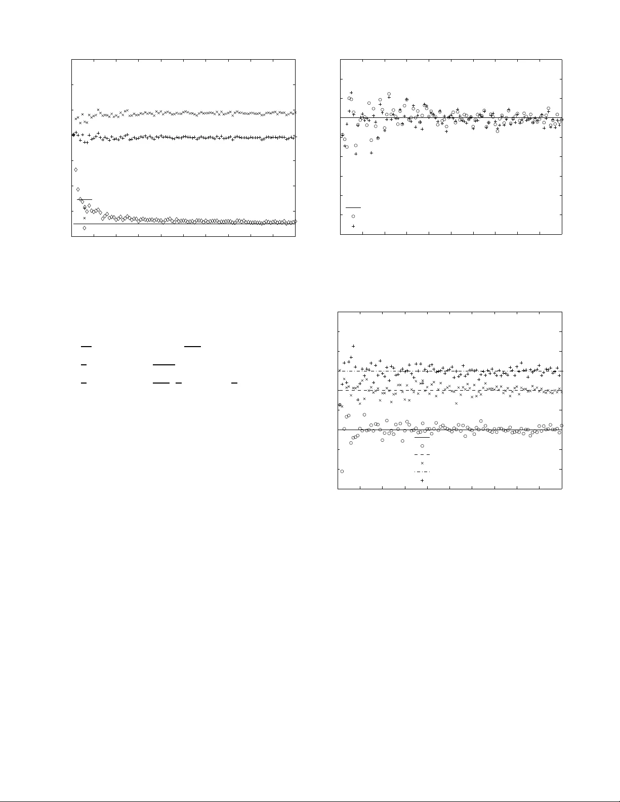
IEEE TRANSACTIONS ON SI GNAL PR OCESSING, V OL. 1, NO. 1, J ANU AR Y 2007 1 Channel Capacity Estimation using Free Probabilit y Theory Øyvind Ryan, Member , I EEE and M ´ erouane Debbah, Member , IEEE Abstract —In many channel measurem ent appli cations, one needs to estimate some characteristics of the channels based on a limited set of measurements. This is mainly due to the highly time vary ing characteristics of the channel. In this contribution, it will be sh own how free probability can b e used fo r chann el capacity estimation in MIM O systems. F ree probability has already been a pplied in v arious application fields such as digital communications, nuclear physics a nd mathematical finance, and has been shown to be an in valuable tool f or describing the asymptotic behaviour of many large-dimensional systems. In particular , using t he concept of f ree decon v olution, we provide an asymptotically (w . r . t. the number of observ ations) unb iased capacity estimator f or MIMO channels impaired with noise called the free probability based estimator . Another estimator , called the Gaussian matrix mean based estimator , is also in troduced by sligh tly modifying t he free p robability based estimator . This estimator is shown to give un biased estimation of the moments of the channel matrix for any number of observ ations. Also, the estimator has this property when we extend to MIMO chann els with p hase off-set and frequency drift, fo r whi ch no estimator has been provided so far in th e literature. It is also sh own that both the free probability based and the Gaussian matrix mean based estimator are asym ptotically unbiased capacity estimators as the n umber of transmit antennas go to infini ty , regardless of wheth er phase off-set and frequency d rift are present. The limitations in the two estimators are also explain ed. Simulations are run to assess th e p erf ormance of the estimators f or a low number of antennas and samples to confirm th e u sefulness of the asymptotic results. Index T erms —Free Probability Theory , Random M atrices, decon volution, limiting eigenv alue distribution, MIMO. I . I N T R O D U C T I O N Random matrices, and in par ticular limit distributions of sample covariance matrices, hav e proved to b e a usefu l tool for modelling systems, for in stance in d igital co mmunic ations [1], nuclear physics [2] and mathematical fina nce [3 ]. A ty pical random matrix mo del is the informatio n-plus-n oise mod el, W n = 1 N ( R n + σ X n )( R n + σ X n ) H . (1) R n and X n are assumed indep endent random matrices of dimension n × N , whe re X n contains i.i.d. standard (i.e . mea n 0 , variance 1 ) co mplex Gaussian entrie s. (1) can be thou ght of as the sample covariance matr ices of random vectors r n + σ x n . This work wa s supporte d by Alcatel-Luc ent within the Alc atel -Lucent Chai r on flexib le radio at SUPELEC This paper was presented in part at the Asilomar Conference on Signals, Systems and Computers, 2007, Pac ific Grov e, USA Øyvind Ryan is with the Centr e of Mathemat ics for Applicat ions, Uni- versi ty of Oslo, P .O. Box 1053 Blindern, NO -0316 Oslo, NOR W A Y , oyvin- dry@ifi.uio.no M ´ erouane Debbah is with SUPELEC, Gif-sur-Yvet te, France, mer- ouane.deb bah@supel ec.fr r n can be interp reted as a vector contain ing the system ch arac- teristics ( direction o f ar riv al for instance in radar application s or imp ulse r esponse in chan nel estimation applications). x n represents add itiv e noise, with σ a measure of the strength of the noise. Classical sign al proc essing estimation m ethods consider the case where the nu mber of ob servations N is highly bigg er than th e dime nsions of th e system n , fo r which equation (1) can be shown to be ap proxima tely: W n = Γ n + σ 2 I n . (2) Here, Γ n is the true c ovariance of the signal. In this case, one can separ ate the signal eige n values fro m the noise ones and inf er (b ased only on the statistics of the sign al) on the characteristics of the input signal. Howev er , in many situations, one can gather on ly a limited nu mber of observations du ring which the characteristics of the signa l d oes not chang e. In order to model this case, n and N will be incr eased so that lim n →∞ n N = c , i.e. the number o f observations is increased at th e same rate as th e num ber of p arameters of the system (note that equa tion ( 2) correspo nds to th e case c = 0 ). Previous contributions hav e alread y dealt with this pr oblem. In [4], Dozier and Silverstein explain h ow one can use the eigenv alue distribution of Γ n = 1 N R n R H n to estimate th e eigenv alue distribution of W n by solv ing a given eq uation. In [5] , [6], we provided an algorithm fo r p assing between the two, using the conc ept of multiplicative free convolution , which ad mits a con venient implemen tation. The implem enta- tion perform s fre e co n volution exactly based solely on mo- ments. In this paper, ch annel capacity e stimation in MI MO systems is used as a bench mark app lication by u sing the connec tion between free pro bability theory and systems of type (1). For MI MO chan nels with and without fre quency off-sets, we derive explicit asym ptotically un biased estimators wh ich perfor m mu ch better th an classical ones. W e do not prove directly that the p ropo sed estimator s work better th an the classical one s, but present simulations which indicate that they are superior . W e rema rk that th e prop osed cap acity estimators will not b e unbiased, it is needed that eithe r the num ber of transmit an tennas or the numbe r of observations be large to obtain p recise estimation . This limitation is most se vere for channels w ith frequen cy o ff-sets, wh ere it is needed in any case that th e number of transmit antenn as is large to o btain precise estimation. A case of stud y where chan nel estimatio n using f ree deconv olution has b een used can be found in [7] and [8]. This paper is organiz ed as follows . Sectio n II p resents th e problem un der conside ration. Sec tion II I provides the b asic IEEE TRANSACTIONS ON SI GNAL PR OCESSING, VOL. 1, NO. 1, J ANU AR Y 2007 2 concepts ne eded on fre e pro bability , inc luding f ree co n vo- lution. In sectio n IV, we f ormalize a new channel cap acity estimator based on free p robability , an d explain some of the shortco mings fo r MIMO models with frequ ency off-sets. Another estimator, called the Gaussian matrix me an based estimator is then fo rmalized to address th e shortcoming s of the free probability based estimator . W e also presen t ar guments for the Gaussian matrix mean based estimator p erform ing be tter than the free p robability based estimator, in some specific cases. These argum ents are, howev er , n ot definite; we d o not prove that one estimator is better than the other f or the cases consider ed. The limitation s of th e estimato rs are also explained. T he low rank of th e ch annel (less than or equal to four ) is the mo st n otable limitation . In section V, simulations of the estimator s are perf ormed an d compare d, where several qu antities are varied, like the noise variance, rank and dimen sions of the chan nel m atrix, and the num ber of observations. In the following, u pper (lower boldface) symbols will b e used for matrices ( column vectors) wherea s lower symbols will rep resent s calar v alu es, ( . ) T will denote tra nspose operator, ( . ) ⋆ conjuga tion and ( . ) H =  ( . ) T  ⋆ hermitian transpose. I n will represent the n × n identity matrix. T r n will den ote the n on-no rmalized tr ace on n × n matrices, while tr n = 1 n T r n denotes the n ormalized trace. Also, we will throug hout the p aper u se c as a shorthand no tation fo r the ratio between th e n umber of rows and the n umber o f c olumns in the rand om matrix model being con sidered. I I . S TA T E M E N T O F T H E P RO B L E M In u sual time varying measureme nt method s for MIMO systems, on e validates mod els [9] by determin ing h ow the model fits with ac tual capacity m easurements. I n this setting , one has to be extremely cautious about the measurement noise, especially for far field measuremen ts where the signal strength can be lower than the noise. The MIMO measured channel in the frequen cy d omain can be modelled by [10 ], [11] ˆ H i = D r i HD t i + σ X i (3) where ˆ H i , H an d X i are respec ti vely the n × m measured MIMO matrix ( n is the numb er of receiving antennas, m is the number of transmitting antenn as), th e n × m MIMO channel and the n × m noise matrix with i.i.d. standard Gaussian entries. No te that we suppose the noise matrix X i to be spatially white. In the realm o f the chan nel measuremen ts under study , th e antenna outputs a re connected to d ifferent RF (Radio Freq uency) chain s. As a con sequence, for the case under stud y , the chann el noise impa irments are ind epend ent from one received anten na to the other . When one RF chain is used, the noise to be consider ed is not white. This case can also be studied within the framework of free d econv o lution but g oes beyon d the scope of the paper . W e suppose that the channel H , although time v ary ing, s tays constant (block fading assumption) du ring L blocks. D r i and D t i are n × n and m × m diagona l matrices which repre sent phase o ff-sets and ph ase drifts (which are im pairmen ts du e to the antennas an d not the channel) at the receiver an d transmitter g iv e n respectively by (these are supp osed to vary on a block basis) D r i = diag[ e j φ i 1 , ..., e j φ i n ] , and D t i = diag[ e j θ i 1 , ..., e j θ t m ] where the ph ases φ i j and θ i j are r andom. W e assume all p hases indepen dent and u niformly distributed. W e will also compare (3) with th e simpler mo del ˆ H i = H + σ X i , (4) which is (3) witho ut phase off-sets an d phase drifts. The capacity per receiving antenna (in the case where the noise is spatially white add itiv e Gaussian and the channel is not known at the transmitter) o f a chann el with channel ma trix H and signal to noise r atio ρ = 1 σ 2 is given by C = 1 n log 2 det  I n + 1 mσ 2 HH H  = 1 n n X l =1 log 2 (1 + 1 σ 2 λ l ) (5) where λ l are the eigen values of 1 m HH H . The problem co nsists therefor e of estimating the eigenv alues of 1 m HH H based on few observations ˆ H i , which is pa ramoun t f or modelling purpo ses. Note that the capac ity expression sup poses that the channel is per fectly kn own at the re ceiv er and no t at the transmitter . In practice, with the noise impairment, the c hannel will never b e estimated perf ectly and th erefore expression (5) is not achie vable. Howe ver, for MIMO modelling purposes, for which the cap acity is often the matching metr ic, one needs to compare the capacity of th e mod el with exp ression ( 5). There are different meth ods actu ally used f or chann el ca- pacity estimation [12], [ 13], [14], [15]. Usual methods discard, throug h an ad-hoc threshold p rocedu re, all c hannels ˆ H i for which the chann el to n oise ratio ( 1 σ 2 tr n ( HH H ) ) is lower than a thresho ld an d then compu te ˜ C ( σ 2 ) = 1 n log 2 det I n + 1 mσ 2 ( 1 M M X i =1 ˆ H i )( 1 M M X i =1 ˆ H i ) H ) ! where M ≤ L is the numb er of channels having a signal to noise ratio higher than the thresho ld. One of the drawback s o f this method is that one will no t analyze the tru e capacity but only th e capacity of the ”good chann els”. Moreover, on e has to limit the chann el measu rement campaign (in ord er to have enoug h ch annels high er than the threshold ) o nly to regions which ar e clo se (in terms o f actual distance) enough to the base station. Other meth ods, in order to hav e a capacity estimation at a giv en signal to noise ratio (different from the measured o ne with noise v arian ce σ 2 ), normalize each c hannel realization ˆ H i and then compu te for a different value of the noise variance σ 2 1 (for example 10 dB ) the capa city estimate ˜ C ( σ 2 1 ) . In the case wher e σ 2 is high and σ 2 1 is low , on e usually finds a high capacity estimate as one measur es only the noise, which is known to have a h igh multiplexing gain. In this co ntribution, we will provide a neat f ramework, based on free decon volution, for channel capacity estimation that circumvents all th e previous dr awbacks. Mo reover , we will deal with m odel (3), for wh ich n o solution has be en provided in th e literature so far . IEEE TRANSACTIONS ON SI GNAL PR OCESSING, VOL. 1, NO. 1, J ANU AR Y 2007 3 I I I . F R A M E W O R K F O R F R E E C O N V O L U T I O N Free probability [16] theo ry has g rown into an en tire field of research thro ugh the pio neering work of V oiculescu in the 1980’ s. Free p robab ility introdu ces an analogy to the concept of ind ependen ce from classical probab ility , which can b e used for n on-co mmutative r andom variables like m atrices. These more ge neral rand om variables are elements in wh at is called a no ncommutative pr obability space . T his can b e defined by a p air ( A, φ ) , where A is a unital ∗ -algebra with un it I , and φ is a n ormalized (i.e. φ ( I ) = 1 ) lin ear function al on A . The elements of A ar e called random v aria bles. In all o ur e xamples, A will con sist o f n × n matrices or r andom matrices. For matrices, φ will be tr n . The unit in these ∗ -alge bras is the n × n identity m atrix I n . Th e an alogy to indepen dence is called freeness: Definition 1: A family of unital ∗ - subalgeb ras ( A i ) i ∈ I will be called a f ree family if    a j ∈ A i j i 1 6 = i 2 , i 2 6 = i 3 , · · · , i n − 1 6 = i n φ ( a 1 ) = φ ( a 2 ) = · · · = φ ( a n ) = 0    ⇒ φ ( a 1 · · · a n ) = 0 . (6) A family o f ran dom variables a i are said to be free if the algebras they g enerate for m a free family . When restricting A to spaces such as m atrices, or fun ctions with bounded supp ort, it is c lear that the momen ts of a uniquely identify a prob ability m easure, h ere called ν a , such that φ ( a k ) = R x k dν a ( x ) . In such spaces, th e d istributions of a 1 + a 2 and a 1 a 2 giv e us two new probab ility measures, which dep end only o n the probab ility m easures associated with a 1 , a 2 when these ar e fr ee. T herefor e we can define two operatio ns on the set of p robability measures: Additive fr ee convolution η 1 ⊞ η 2 for th e sum of free r andom variables, and multiplicative free convolution η 1 ⊠ η 2 for the pr oduct of free r andom variables. These o perations can in many cases be used to p redict the spectrum of sums or products of large random matrices: If a 1 n has an eigenv alue d istribution which approa ches η 1 and a 2 n has an eige n value distribution which approa ches η 2 , then in many cases th e eigenvalue d istribution of a 1 n + a 2 n approa ches η 1 ⊞ η 2 . One importan t pr obability measure is the Mar ˘ chenko Pastur law µ c [17], which has the d ensity f µ c ( x ) = (1 − 1 c ) + δ 0 ( x ) + p ( x − a ) + ( b − x ) + 2 π cx , (7) where ( z ) + = max (0 , z ) , a = (1 − √ c ) 2 , b = (1 + √ c ) 2 , and δ 0 ( x ) is dir ac measure (poin t mass) at 0 . Accordin g to the notation in [18], µ c is also the free Poisson distribution with rate 1 c and jump size c . W e will need the following form ulas for the first m oments of the Mar ˘ chenko Pastur law: R xf µ c ( x ) dx = 1 R x 2 f µ c ( x ) dx = c + 1 R x 3 f µ c ( x ) dx = c 2 + 3 c + 1 R x 4 f µ c ( x ) dx = c 3 + 6 c 2 + 6 c + 1 . (8) (8) follows immed iately from applying wha t is called th e moment-cu mulant formula [1 8], to the free cu mulants [18] of th e Mar ˘ chenko Pastur law µ c . The (fr ee) cu mulants of the Mar ˘ chenko Pastur law are 1 , c, c 2 , c 3 , ... [5]. Cumu lants and the moment- cumulant f ormula in free p robability have analogo us concep ts in classical p robab ility . µ c describes asymptotic eigenv alue distributions of W ishart matrices , i.e. m atrices on th e form 1 N RR H , with R an n × N random matrix with indepe ndent standard complex Gaussian entries, an d n N → c . This ca n be seen fro m the following result, where the difference fro m (8) vanishes when N → ∞ : Pr oposition 1: Let X n be a complex standard Gaussian n × N matrix , an d set c = n N . Then E  tr n  1 N X n X H n  = 1 E h tr n   1 N X n X H n  2 i = c + 1 E h tr n   1 N X n X H n  3 i = c 2 + 3 c + 1 + 1 N 2 E h tr n   1 N X n X H n  4 i = c 3 + 6 c 2 + 6 c + 1 + 5(1+ c ) N 2 . (9) This will b e u seful later on whe n we compu te mixed mo ments of Gaussian and deterministic matrices. The proo f of pro posi- tion 1 is given in a ppendix B. W e will also find it u seful to in troduce the co ncept of multiplicative fr ee deconvolution : Giv e n probab ility me asures η an d η 2 . Whe n there is a uniqu e probab ility measure η 1 such that η = η 1 ⊠ η 2 , we will write η 1 = η r η 2 , an d say that η 1 is the multiplicative free deconv o lution of η with η 2 . There is n o rea son why a probab ility m easure shou ld h av e a unique deconv o lution, and whether on e exists at all d epends highly on the p robab ility measure η 2 which we d econv olve with. This will not be a pr oblem for our purpo ses: First o f all, we will only have n eed f or multiplicative f ree deconv o lution with µ c , and only in or der to find the mom ents of the channel matrix. The pr oblem of a uniqu e deconv olu tion is there fore addr essed by an existing algo rithm for f ree deco n volution [6], which finds u nique mo ments o f η r µ c (as long as the first moments of η is no nzero). W e will need the following d efinitions: Definition 2: By the empirical eigenvalue distrib ution o f an n × n random ma trix X we mean the r andom ato mic measur e 1 n  δ λ 1 ( X ) + · · · + δ λ n ( X )  , where λ 1 ( X ) , ..., λ n ( X ) are the (ran dom) eigen values of X . Definition 3: A sequ ence of rand om variables a n 1 , a n 2 , ... in p robab ility spaces ( A n , φ n ) is said to conv erge in distri- bution if, f or any m 1 , ..., m r ∈ N , k 1 , ..., k r ∈ { 1 , 2 , ... } , we have that the limit φ n ( a m 1 nk 1 · · · a m r nk r ) exists as n → ∞ . T o make the c onnection between m odels (4), (3) and mo del (1), we need the following re sult [5]: Theor em 1 : Assum e that the empirical eig en value distri- bution of Γ n = 1 N R n R H n conv erges in distribution almost surely to a comp actly supported prob ability measure η Γ . Then we have tha t the em pirical eig en value distribution of W n also converges in distribution almo st surely to a compa ctly supported probab ility me asure η W uniquely identified b y η W r µ c = ( η Γ r µ c ) ⊞ δ σ 2 , (10) where δ σ 2 is dirac measure (p oint mass) at σ 2 . IEEE TRANSACTIONS ON SI GNAL PR OCESSING, VOL. 1, NO. 1, J ANU AR Y 2007 4 Theorem 1 can also be r e-stated (th rough deco n volution ) as η W = (( η Γ r µ c ) ⊞ δ σ 2 ) ⊠ µ c . When we h av e L obser vations ˆ H i in a MIMO system as in (4) or (3), we will f orm the n × mL random ma trices ˆ H 1 ...L = H 1 ...L + σ √ L X 1 ...L (11) with ˆ H 1 ...L = 1 √ L h ˆ H 1 , ˆ H 2 , ..., ˆ H L i , H 1 ...L = 1 √ L  D r i HD t i , D r i HD t i , ..., D r i HD t i  , X 1 ...L = [ X 1 , X 2 , ..., X L ] . This is the way w e will stack the ob servations in this p aper . It is o nly one of many po ssible stacking s. A stacking where the ratio between th e n umber of rows and the n umber o f c olumns conv erges to a quantity between 0 and 1 would allow us to use theorem 1 (which imp licitly assumes 0 < c < 1 ) directly to conclud e alm ost sure convergence, which a gain would help us to conclu de that the introd uced capacity estimators are asymptotically u nbiased. Such a stacking can also reduce the variance of the estimators. Even though the stack ing considered here may no t give the lowest variance, and m ay not give almost sure con vergence, we show th at its variance conv erges to 0 and provides asymp totic unb iasedness for the correspo nding capacity estimato r . For th e case L = 1 , the f ormula tr n   D r 1 HD t 1  D r 1 HD t 1  H  j  = tr n   HH H  j  (12) can be com bined with theorem 1 to give the appr oximation ν 1 m ˆ H 1 ˆ H H 1 r µ n m ≈  ν 1 m HH H r µ n m  ⊞ δ σ 2 . (13) for a single ob servation. This approxim ation works well when n is large. For many o bservations, note that H 1 ...L H H 1 ...L = HH H when there is no p hase off-set an d pha se d rift, so that the app roximatio n ν 1 m ˆ H 1 ...L ˆ H H 1 ...L r µ n mL ≈  ν 1 m HH H r µ n mL  ⊞ δ σ 2 (14) applies and gener alizes (13). The ratio between the num ber of rows an d colu mns in the matrices H 1 ...L , X 1 ...L and ˆ H 1 ...L is c = n mL , con sidering the horizon tal stacking of the observa- tions in a larger matrix. It is on ly th is stack ing wh ich will be considered in this pap er . When phase off-set a nd p hase drift are add ed, it is much harder to adapt theorem 1 to pr oduce the moments of 1 m HH H . The reason is that theo rem 1 really h elps us to find the moments of 1 m H 1 ...L H H 1 ...L . In th e case with out phase off- set and phase d rift, this is enough since these mom ents are equal to the moments of 1 m HH H . However , eq uality be tween these mom ents does not ho ld when pha se off-set an d phase drift are ad ded. A pro cedure f or converting b etween these moments may exist, but seems to be r ather com plex, and will n ot be dealt with here. In sectio n IV, we will instead define a n estimator f or th e cha nnel c apacity which d oes no t stack observations into th e matrix H 1 ...L at all. Instead , an estimation will be perfor med for each ob servation, takin g th e mean of all the estimates at the end. I V . N E W E S T I M A T O R S F O R C H A N N E L C A PAC I T Y In this section, two new channel capa city estimators are defined. Fir st, a fr ee pr o bability based estimator is introdu ced, which (for m odel (4)) w ill be shown to be asymp totically unbiased w .r .t. the nu mber o f observations. The n, by slightly modify ing the free prob ability based estimator , we will con- struct what we call the Gaussian matrix me an based capacity estimator . This estimator will be shown, for model (4) and (3), to giv e u nbiased estimates of the mom ents of th e chann el matrix for any num ber of ob servations. The c omputatio nal complexity f or the two estimators lies in the com putation of eigenv alues and momen ts of the matrix HH H , in addition to computin g the free (d e)conv o lution in ter ms of mo ments. For th e matr ix ranks co nsidered here, fre e (de )conv olu tion requires few computation s. The complexity in the comp utation of eigenv alu es and mo ments of th e matrix HH H grows with n (the number of receiving an tennas), which is small in this paper . The computational co mplexity in the estimato rs grows slowly with the number of obser vations, since the dimen sions of ˆ H 1 ...L ˆ H H 1 ...L does no t grow with L . The two estimators are stated as estimators for the lower order moments of 1 m HH H . Under the assumptio n th at this matrix h as lim ited rank (such as ≤ 4 here), estimator s f or lower o rder m oments can be used to define estimato rs fo r the chan nel capacity , since th e capacity can be written as a function of th e r lowest moments when the matrix h as rank r , as explained below . A. Th e fr ee pr obability ba sed capacity estimator The f ree pro bability based estimator is define d as follows: Definition 4: The f ree p robab ility based estimator for the capacity of a chann el with channel matrix H of ran k r , denoted C f , is comp uted through the following steps: 1) Compu te the first r mo ments ˆ h 1 , ..., ˆ h r of the samp le covariance m atrix 1 m ˆ H 1 ...L ˆ H H 1 ...L (i.e. compu te ˆ h j = tr n   1 m ˆ H 1 ...L ˆ H H 1 ...L  j  for 1 ≤ j ≤ r ), 2) use (1 4) to estimate the first r mome nts h f 1 , ..., h f r of 1 m HH H , 3) estimate the r nonzero eigen values λ 1 , ..., λ r of 1 m HH H from h f 1 , ..., h f r . Substitute these in ( 5). W e also call h f 1 , ..., h f r the free p robability based estimator s for the r first momen ts o f 1 m HH H . Steps 2 and 3 in definitio n 4 need some elabo ration. T o address step 3, con sider the case of a rank 3 channel matrix. For such ch annel matrices, only th e lowest th ree mom ents h 1 , h 2 , h 3 of 1 m HH H need to be estimated in order to estimate the eigenv alues. T o see this, first w rite C = 1 n log 2 det  I n + 1 mσ 2 HH H  = 1 n log 2  1 + 1 σ 2 λ 1   1 + 1 σ 2 λ 2   1 + 1 σ 2 λ 3  , (15) where λ 1 , λ 2 and λ 3 are the three non -zero eigenv alues of 1 m HH H . This qu antity can easily b e calculated from the IEEE TRANSACTIONS ON SI GNAL PR OCESSING, VOL. 1, NO. 1, J ANU AR Y 2007 5 elementary symmetric polyn omials Π 1 ( λ 1 , λ 2 , λ 3 ) = λ 1 + λ 2 + λ 3 Π 2 ( λ 1 , λ 2 , λ 3 ) = λ 1 λ 2 + λ 2 λ 3 + λ 1 λ 3 Π 3 ( λ 1 , λ 2 , λ 3 ) = λ 1 λ 2 λ 3 . by observ ing th at  1 + 1 σ 2 λ 1   1 + 1 σ 2 λ 2   1 + 1 σ 2 λ 3  can be written as 1 + 1 σ 2 Π 1 ( λ 1 , λ 2 , λ 3 ) + 1 σ 4 Π 2 ( λ 1 , λ 2 , λ 3 ) + 1 σ 6 Π 3 ( λ 1 , λ 2 , λ 3 ) . (16) Π 1 ( λ 1 , λ 2 , λ 3 ) can in turn be ca lculated fro m the power polyno mials S 1 ( λ 1 , λ 2 , λ 3 ) = λ 1 + λ 2 + λ 3 = ntr n  1 m HH H  S 2 ( λ 1 , λ 2 , λ 3 ) = λ 2 1 + λ 2 2 + λ 2 3 = ntr n   1 m HH H  2  S 3 ( λ 1 , λ 2 , λ 3 ) = λ 3 1 + λ 3 2 + λ 3 3 = ntr n   1 m HH H  3  by using the Newton-Girar d formulas [19], w hich for the th ree first mo ments take the form Π 1 = S 1 , Π 2 = 1 2  S 2 1 − S 2  and Π 3 = 1 6  S 3 1 − 7 S 1 S 2 + 2 S 3  . If the ch annel m atrix h as a higher rank r , sim ilar reasoning can be used to conclud e that the fir st r moments need to be estimated. In the simulations, the eigen values th emselves are never compu ted, since com pu- tation of the moments and th e Newton-Girard form ulas make this unne cessary . T o addr ess step 2 in defin ition 4, a Matlab impleme nta- tion [ 20] which perfo rms free (de)c onv olutio n in terms of moments a s describ ed in [6] was d ev eloped and u sed f or the simulations in th is pap er . Free (d e)conv o lution is computation- ally e xpensive for higher order moments o nly: F or the first four moments, step 2 in definition 4 is equiv alent to the following: Pr oposition 2: Let ˆ h 1 , ˆ h 2 , ˆ h 3 , ˆ h 4 and h f 1 , h f 2 , h f 3 , h f 4 be as in defin ition 4 . Then ˆ h 1 = h f 1 + σ 2 ˆ h 2 = h f 2 + 2 σ 2 (1 + c ) h f 1 + σ 4 (1 + c ) ˆ h 3 = h f 3 + 3 σ 2 (1 + c ) h f 2 + 3 σ 2 ch 2 f 1 +3 σ 4  c 2 + 3 c + 1  h f 1 + σ 6  c 2 + 3 c + 1  ˆ h 4 = h f 4 + 4 σ 2 (1 + c ) h f 3 + 8 σ 2 ch f 2 h f 1 + σ 4 (6 c 2 + 16 c + 6) h f 2 +14 σ 4 c (1 + c ) h 2 f 1 +4 σ 6 ( c 3 + 6 c 2 + 6 c + 1) h f 1 + σ 8  c 3 + 6 c 2 + 6 c + 1  , (17) where c = n mL . The proo f of pro position 2 can be fou nd in ap pendix A. The f ollowing is the main r esult on the f ree p robability based estimator , and covers the different cases for bias a nd asymptotic bias w .r .t. numb er o f observations or an tennas. Theor em 2 : For L = 1 observation, the fo llowing h olds for both mod els ( 3) a nd (4): 1) h f 1 and h f 2 are unbiased. h f 3 and h f 4 are biased, with the bias of h f 3 giv en b y − 3 σ 4 tr n  1 m HH H  + σ 6 m 2 . In par ticular h f 3 and h f 4 are asymp totically unbia sed when m → ∞ (with n, L kept fixed) , i.e. lim m →∞ E ( h f j ) = tr n  1 m HH H  j ! , 3 ≤ j ≤ 4 . 2) C f is asympto tically u nbiased when m → ∞ ( with n, L kept fixed) and 1 m HH H has ran k ≤ 4 , i.e. lim m →∞ C f = C . For any numbe r of observations L with mo del (4), the follow- ing holds: 1) h f 1 and h f 2 are unbiased. h f 3 and h f 4 are biased, with the bias of h f 3 giv en by − 3 σ 4 tr n  1 m HH H  + σ 6 m 2 L 2 . In par ticular h f 3 and h f 4 are asymp totically unbia sed when either m → ∞ or L → ∞ (with the other kept fixed), i.e. lim m →∞ E ( h f j ) = lim L →∞ E ( h f j ) = tr n  1 m HH H  j ! for 3 ≤ j ≤ 4 . 2) C f is asymp totically unb iased when either m → ∞ (with n, L kept fixed), or L → ∞ ( with m, n kept fixed) and 1 m HH H has rank ≤ 4 , i.e. lim m →∞ C f = lim L →∞ C f = C . The proof of theor em 2 can be foun d in append ix C. Th e bias in th eorem 2 motivates the defin ition o f the estimator of the next section. Th e free prob ability based estimator perfo rms estimation as if the Gaussian rando m matrices and determ inis- tic matrices in volved were free. It turns out that these matrices are on ly asymptotically fr ee [16], which explain s why there is a bias inv olved, and why the b ias decreases as the matrix dimensions increase. B. Th e Gaussian matrix mean b ased capa city estimator The exp ression for th e Gau ssian matrix mean b ased capac- ity estimato r is mo ti vated fro m co mputing expected values of mixed mo ments of Gaussian and dete rministic matrices (lemma 1). This results in expressions slightly different fro m (17). W e will show th at the Gaussian matrix mean based estimator can be used fo r channe l ca pacity estimatio n in ce r- tain sy stems where the free pr obability ba sed estimato r fail s. The definition of the Gaussian matrix mean based ca pacity estimator is as follows for matrices of ra nk ≤ 4 : Definition 5: The Gaussian matrix mea n b ased estimato r for th e capacity of a channel with channel m atrix H of rank r ≤ 4 , den oted C G , is defined thro ugh the following steps: 1) For each observation, per form the following a) Compute the first r m oments ˆ h i 1 , ..., ˆ h ir of the sample covariance matrix 1 m ˆ H i ˆ H H i (i.e. comp ute ˆ h ij = tr n   1 m ˆ H i ˆ H H i  j  for 1 ≤ j ≤ r ), IEEE TRANSACTIONS ON SI GNAL PR OCESSING, VOL. 1, NO. 1, J ANU AR Y 2007 6 b) find estimates h i 1 , h i 2 , h i 3 , h i 4 of the first four moments of 1 m HH H by solving ˆ h i 1 = h i 1 + σ 2 ˆ h i 2 = h i 2 + 2 σ 2 (1 + c ) h i 1 + σ 4 (1 + c ) ˆ h i 3 = h i 3 + 3 σ 2 (1 + c ) h i 2 + 3 σ 2 ch 2 i 1 +3 σ 4  c 2 + 3 c + 1 + 1 m 2  h i 1 + σ 6  c 2 + 3 c + 1 + 1 m 2  ˆ h i 4 = h i 4 + 4 σ 2 (1 + c ) h i 3 + 8 σ 2 ch i 2 h i 1 + σ 4 (6 c 2 + 16 c + 6 + 16 m 2 ) h i 2 +14 σ 4 c (1 + c ) h 2 i 1 +4 σ 6 ( c 3 + 6 c 2 + 6 c + 1 + 5( c +1) m 2 ) h i 1 + σ 8  c 3 + 6 c 2 + 6 c + 1 + 5( c +1) m 2  , (18) where c = n m , Form the estimates h uj = 1 L P L i =1 h ij , 1 ≤ j ≤ r , of the first mo ments o f 1 m HH H , 2) estimate the r nonzero eigenv alu es λ 1 , ...λ r of 1 m HH H from h u 1 , ..., h ur . Substitute these in ( 5). W e also call h u 1 , ..., h ur the Gau ssian matrix mean ba sed estimators for the r first m oments of 1 m HH H . While a Matlab implementatio n [20] of free (de )conv olu tion is u sed for the f ree ( de)conv olution in the fr ee p robability based estimator, the algorithm f or the Gaussian matrix m ean based cap acity estimator used by the simulations in this pap er follows the step s in definition 5 dir ectly . Note that (18) resemb le the formulas in ( 17) when c = n m . c = n m is used in definition 5 since the observation matrices ˆ H i are not stacked togeth er in a larger matrix in this c ase. Instead, a mean is taken of all estimated moments in step 1 of the definition. This is not an o ptimal proced ure, and we u se it only b ecause it is hard to comp ute mixed moments of matrices where observations ˆ H i of type (3) ar e stacked together . The following theorem is the main result on the Gaussian matrix mean b ased estimato r , and sh ows that it qua lifies for it’ s name. Theor em 3 : For either model (4) o r (3), th e following hold s: 1) The estimator s h u 1 , h u 2 , h u 3 , h u 4 are unbiased, i.e. E ( h uj ) = tr n  1 m HH H  j ! , 1 ≤ j ≤ 4 . 2) C G is asympto tically unbiased as m → ∞ (with n, L kept fixed) when 1 m HH H has rank ≤ 4 , i.e. lim m →∞ C G = C . 3) In the ca se of L = 1 observation, h f 1 = h u 1 and h f 2 = h u 2 . In par ticular, C f = C G when 1 m HH H has rank ≤ 2 . The proo f of th eorem 3 can be found in appendix C. C. Limitations of the two estimato rs W e have c hosen to d efine two estimators, sinc e they have different limitation s. The most severe limitation of the G aussian matrix m ean based capa city estimator, th e way it is defined , lies in the restriction on the rank. This restriction is done to limit the complexity in the expression for the estimator . Howe ver, the computatio ns in appen dix C sho uld convince the read er that capacity estimator s with similar pro perties can b e written down (howe ver complex) fo r higher rank chan nels also . Also, while th e fr ee pr obability based estimato r h as an algorithm [6] for ch annel matrices of any rank, th ere is no reason why a similar alg orithm can not be fou nd for the Gau ssian matrix mean based estimator also. Th e computation s in ap pendix C indicate that such an algo rithm sho uld be based solely on iteration thro ugh a finite set of partitions. How this can be done algorithm ically is b eyond the scope o f this paper . For the free pro bability based estimator the lim itation lies in the presen ce of ph ase off-set an d phase dr ift (model (3)): When model (3) is used, the commen ts at the end of section III make it clear that we lack a relation for obtaining the mo ments of 1 m H 1 ...L H H 1 ...L from th e momen ts of 1 m HH H . W itho ut such a r elation, we also h ave no candida te fo r a cap acity estimator (capacity estimators in this paper are motiv ated by first finding moment estimator s). In conclusion, the stacking of observations performed by the f ree pro bability based estimator does not work for m odel (3). Only the Gaussian matrix mean based estimator can perfo rm reliable capa city estimation f or many observations with model (3). The second limitation of the free p robab ility based estimator comes from the inherent bias in its deconv olution formu las (17). The bias is on ly large when both m and L are sma ll (see the orem 2 ), so this point is less sev ere (however , ch annel m atrices d own to size 4 × 4 occur in p ractice). The bias in the lower ord er m oments is easily seen to affect capacity estimation from the fo llowing expansion of th e capacity C = 1 ln 2 P ∞ k =1 ( − 1) k +1 m k ρ k k , (19) which can be obtain ed fro m substitutin g th e T aylor expansion log 2 (1 + t ) = 1 ln 2 ∞ X k =1 ( − 1) k +1 t k k (20) into the definition of the cap acity . Her e ρ = 1 /σ 2 is SNR, and m k are the mo ments of 1 m HH H . It is clear from ( 19) that, at least if we restrict to small ρ , the expression is dom inated by the co ntribution from the first ord er m oments. If m is small we th erefore first ha ve a high relati ve error in the first moments af ter the deconv o lution step, which will p ropaga te to a high relative error in the cap acity estimate for small ρ du e to ( 19). Thus, fre e p robability b ased ca pacity estimation will work p oorly for small m, L and ρ . The same limitation is not present in th e Gaussian m atrix mean based estimator, since its moment estimators are u nbiased. The limitation on the rank can in some cases be av oid ed, if we instead have s ome bound s on the eigen values: If we instead knew that at most four of the eigenv alues ar e not ”negligib le”, we cou ld still use pro position 2 to estimate the capacity . This follows f rom r esults on the con tinuity of multiplicative fre e conv olu tion, wh ich ha s been covered in [2 1]. Such continu ity issues are also beyon d the scop e of this paper . V . C H A N N E L C A PAC I T Y E S T I M AT I O N Sev e ral candidates for chann el capacity estimators for ( 4) have b een used in the literature. W e will con sider the follow- IEEE TRANSACTIONS ON SI GNAL PR OCESSING, VOL. 1, NO. 1, J ANU AR Y 2007 7 0 10 20 30 40 50 60 70 80 90 100 0.2 0.4 0.6 0.8 1 1.2 1.4 1.6 Number of observations Capacity True capacity C 1 C 2 C 3 Fig. 1. Comparison of variou s classical capacity estimators for vario us number of observ ations, model (4). σ 2 = 0 . 1 , n = 10 rec eiv e antennas, m = 10 transmit antennas. The rank of H was 3 . ing: C 1 = 1 nL P L i =1 log 2 det  I n + 1 mσ 2 ˆ H i ˆ H H i  C 2 = 1 n log 2 det  I n + 1 Lσ 2 m P L i =1 ˆ H i ˆ H H i  C 3 = 1 n log 2 det  I n + 1 σ 2 m ( 1 L P L i =1 ˆ H i )( 1 L P L i =1 ˆ H i ) H )  (21) These will be com pared with th e free probability based ( C f ) and the Gaussian m atrix mean based ( C G ) estimators. A. Cha nnels without pha se o ff-set an d p hase drift In figure 1, C 1 , C 2 and C 3 are comp ared for v arious number of o bservations, with σ 2 = 0 . 1 , and a 10 × 10 ch annel matrix of rank 3. It is seen that on ly the C 3 estimator gives v alu es close to the true capacity . The channel considered has no phase drift or phase off-set. C 1 and C 2 are seen to hav e a high bias. In figure 2, th e same σ and chan nel matrix are put to the test with the free- probab ility based and Gaussian m atrix mean based estimators fo r various numb er of o bservations. These giv e v alues close to the true capacity . Bo th work better than C 3 for small numb er of o bservations. The free- probab ility based estimator conver g es faster (in terms of th e n umber of ob servations) f or lo wer rank channel matrices. In figu re 3 we illustrate this fo r 10 × 10 channel matrices of rank 3, 5 and 6. Simulatio ns show that for channel matrices of lower dim ension (fo r instanc e 6 × 6 ), we have slower conver gence to the tru e capacity . B. Cha nnels with pha se off-set and pha se drift In figu re 4, the C 3 estimator is co mpared with the free- probab ility based estimator, the Gaussian matrix mean b ased estimator an d th e true capacity , for v ar ious num ber of obser - vations, and with the same σ and chann el matrix as in figur e 1 and 2. Pha se o ff-set and p hase d rift h av e also been introdu ced. 0 10 20 30 40 50 60 70 80 90 100 0 0.05 0.1 0.15 0.2 0.25 0.3 0.35 0.4 Number of observations Capacity True capacity C f C G Fig. 2. Comparison of C f and C G for vari ous number of observ ations, model (4). σ 2 = 0 . 1 , n = 10 recei ve antennas, m = 10 transmit antennas. The rank of H wa s 3 . 0 10 20 30 40 50 60 70 80 90 100 0 0.1 0.2 0.3 0.4 0.5 0.6 0.7 0.8 0.9 Number of observations Capacity True capacity, rank 3 C f , rank 3 True capacity, rank 5 C f , rank 5 True capacity, rank 6 C f , rank 6 Fig. 3. C f for v arious number of observat ions, model (4 ). σ 2 = 0 . 1 , n = 10 recei ve antenna s, m = 10 transmit antenn as. The rank of H was 3 , 5 and 6 . In this case, the free-pro bability based estimato r an d the C 3 - estimator seem to be biased. In figure 5, simulations have been perfo rmed for various σ . Only L = 1 observation was used, n = 10 receive antennas, and m = 1 0 transmit a ntennas. The channel m atrix has ran k 3 . It is seen th at the Gaussian matr ix mean based c apacity estimator is very clo se to the true capacity , There ar e only small deviations ev en if o ne o bservation is present, wh ich provides a very go od ca ndidate for chan nel estima tion in highly time -varying en viro nments. The deviations are higher for high er σ . In figu re 6 we have also varied σ and used on ly one observation, but we h ave for med anoth er ra nk 3 matrix with, n = 4 receive anten nas, m = 4 transmit antenn as. It is seen that th e deviation from the tr ue ca pacity is mu ch higher in this case. W e have in figure 7 increased the number of observations IEEE TRANSACTIONS ON SI GNAL PR OCESSING, VOL. 1, NO. 1, J ANU AR Y 2007 8 0 10 20 30 40 50 60 70 80 90 100 0 0.05 0.1 0.15 0.2 0.25 0.3 0.35 0.4 Number of observations Capacity True capacity C 3 C f C G Fig. 4. Comparison of capac ity estimat ors which wor ked for model (4) for increa sing number of observa tions. Model (3) is used. σ 2 = 0 . 1 , n = 10 recei ve antennas, m = 10 transmit antenna s. The rank of H wa s 3 . 0.05 0.1 0.15 0.2 0.25 0.3 0.35 0.4 0.45 0.5 −1 −0.5 0 0.5 1 1.5 2 2.5 σ Capacity True capacity C G Fig. 5. C G for L = 1 observ ation, n = 10 recei ve anten nas, m = 10 transmit antennas, with varying val ues of σ . Model (3). The rank of H was 3 . to 10 , and used the same chann el matrix. I t is seen that this decreases the deviation from the true cap acity . Finally , let us u se a ch annel matrix of rank 4 . In this case we h av e to increa se the num ber o f observations even further to accurately pr edict th e chan nel c apacity . In figure 8, Gaussian matrix mea n based capac ity estimation is perform ed for a rank 4 channe l matrix with n = 4 receive antennas, m = 4 transmit an tennas. 1 o bservation is perf ormed. If we increase the n umber o f o bservations, Gaussian m atrix mea n based ca pacity estimation is seen to go very slowly towards the true c apacity . T o illustrate this, figure 9 sh ows Gaussian matrix m ean based cap acity estimation for 10 observations on the same cha nnel matrix. It is seen th at this d ecreases the deviation fro m the true c apacity . 0.05 0.1 0.15 0.2 0.25 0.3 0.35 0.4 0.45 0.5 −1 0 1 2 3 4 5 6 7 σ Capacity True capacity C G Fig. 6. C G for L = 1 o bserv ation, n = 4 recei ve antennas, m = 4 tra nsmit antenna s , with varyin g v alues of σ . Model (3). The rank of H was 3 . 0.05 0.1 0.15 0.2 0.25 0.3 0.35 0.4 0.45 0.5 0 1 2 3 4 5 6 7 σ Capacity True capacity C G Fig. 7. C G for L = 1 0 observa tions, n = 4 recei ve anten nas, m = 4 transmit antennas, with varying val ues of σ . Model (3). The rank of H was 3 . V I . C O N C L U S I O N In th is p aper, we have shown that free p robab ility p rovides a neat framework for estimating th e chan nel capacity fo r certain M IMO systems. In the case of h ighly time varying en vironmen ts, where one can rely only on a set of limited no isy measuremen ts, we hav e provided an asymptotically unbiased estimator of the ch annel ca pacity . A mod ified estimator called the Gaussian m atrix mean based estimator was also introdu ced to take into account th e bia s in the case of finite dimen sions and was proved to be a dequate for low rank channe l matrices. Moreover , although the results are based on asymptotic claims (in the n umber of observations), simu lations show that the estimators work well for a very low number of observations also. Even when considering discrepancies such as phase drif ts and phase o ff-set, the algorithm, based o n th e Gaussian m atrix IEEE TRANSACTIONS ON SI GNAL PR OCESSING, VOL. 1, NO. 1, J ANU AR Y 2007 9 0.05 0.1 0.15 0.2 0.25 0.3 0.35 0.4 0.45 0.5 0 1 2 3 4 5 6 7 8 9 σ Capacity True capacity C G Fig. 8. C G for L = 1 o bserv ation, n = 4 rec eiv e antennas, m = 4 transmit antenna s , with v arying v alues of σ . Model (3). The rank of H was 4 . 0.05 0.1 0.15 0.2 0.25 0.3 0.35 0.4 0.45 0.5 0 1 2 3 4 5 6 7 8 9 σ Capacity True capacity C G Fig. 9. C G for L = 1 0 observa tions, n = 4 recei ve antennas, m = 4 transmit antennas, with varying val ues of σ . Model (3). The rank of H was 4 . mean b ased estimator, pr ovided very g ood per forman ce. Fur- ther research is bein g conducted to take into ac count spatial correlation of th e noise (in other word s, deconv o lving with other measur es th an the Mar ˘ chenko Pastur law). A P P E N D I X A T H E P RO O F O F P RO P O S I T I O N 2 Let ( m 1 , m 2 , ... ) be the moments of η , ( M 1 , M 2 , ... ) the moments of η ⊠ µ c . Then [6] cM 1 = cm 1 cM 2 = cm 2 + c 2 m 2 1 cM 3 = cm 3 + 3 c 2 m 1 m 2 + c 3 m 3 1 cM 4 = cm 4 + 4 c 2 m 1 m 3 + 2 c 2 m 2 2 + 6 c 3 m 2 1 m 2 + c 4 m 4 1 . (22) Note that (22) can also be inv erted to expre ss the m j in terms of the M j instead: cm 1 = cM 1 cm 2 = cM 2 − c 2 M 2 1 cm 3 = cM 3 − 3 c 2 M 1 M 2 + 2 c 3 M 3 1 cm 4 = cM 4 − 4 c 2 M 1 M 3 − 2 c 2 M 2 2 + 10 c 3 M 2 1 M 2 − 5 c 4 M 4 1 . (23) Note also that th e moments of η ⊞ δ σ 2 are m 1 + σ 2 m 2 + 2 σ 2 m 1 + σ 4 m 3 + 3 σ 2 m 2 + 3 σ 4 m 1 + σ 6 m 4 + 4 σ 2 m 3 + 6 σ 4 m 2 + 4 σ 6 m 1 + σ 8 (24) By the definition o f the free prob ability based estimator, ν 1 m ˆ H 1 ...L ˆ H H 1 ...L =  η r µ 1 L  ⊞ δ σ 2  ⊠ µ 1 L where the moments of η are h 1 , h 2 , h 3 , ... . Deno ting by η 1 = η r µ 1 L , η 2 = η 1 ⊞ δ σ 2 , we have that ν 1 m ˆ H 1 ...L ˆ H H 1 ...L = η 2 ⊠ µ 1 L . Denote also the mome nts of η 1 by r i , the momen ts of η 2 by s i , and as before the moments of 1 m ˆ H 1 ...L ˆ H H 1 ...L by ˆ h 1 , ˆ h 2 , ˆ h 3 , ... . Write also c = n mL as in prop osition 2. For the third mo ment, we can app ly (2 2), (24) and (2 3) in that order, ˆ h 3 = s 3 + 3 cs 1 s 2 + c 2 s 3 1 = r 3 + 3 σ 2 r 2 + 3 σ 4 r 1 + σ 6 +3 c ( r 1 + σ 2 )( r 2 + 2 σ 2 r 1 + σ 4 ) + c 2 ( r 1 + σ 2 ) 3 = r 3 + 3 cr 1 r 2 + c 2 r 3 1 +3 σ 2 (1 + c ) r 2 + (6 c + 3 c 2 ) σ 2 r 2 1 + σ 4 (3 + 9 c + 3 c 2 ) r 1 + σ 6 (1 + 3 c + c 2 ) = h 3 − 3 ch 1 h 2 + 2 c 2 h 3 1 +3 ch 1 ( h 2 − ch 2 1 ) + c 2 h 3 1 +(6 c + 3 c 2 ) σ 2 h 2 1 + 3 σ 2 (1 + c )( h 2 − ch 2 1 ) + σ 4 (3 + 9 c + 3 c 2 ) h 1 + σ 6 (1 + 3 c + c 2 ) = h 3 + 3 σ 2 (1 + c ) h 2 + 3 σ 2 ch 2 1 +3 σ 4  c 2 + 3 c + 1  h 1 + σ 6  c 2 + 3 c + 1  , which is th e third equation in (17) of p roposition 2. Calcula- tions are similar f or the o ther momen ts, but more tedio us for the fourth mome nt. A P P E N D I X B T H E P RO O F O F P RO P O S I T I O N 1 In all th e follo wing, the matrices are of dim ension n × N . W e need some terminolog y and results fro m [ 22] for th e pr oof of propo sition 1. Let S p be the set of p ermutation s o f p e lements { 1 , 2 , ..., p } . For π ∈ S p , let also ˆ π be th e per mutation in S 2 p defined by ˆ π (2 j − 1) = 2 π − 1 ( j ) , ( j ∈ { 1 , 2 , ..., p } ) ˆ π (2 j ) = 2 π ( j ) − 1 , ( j ∈ { 1 , 2 , ..., p } ) , (25) let ∼ ˆ π denote the eq uiv alen ce relation on { 1 , ..., 2 p } generated by the expression j ∼ ˆ π ˆ π ( j ) + 1 , (add ition formed mod. 2 p ) , (26) and let k ( ˆ π ) and l ( ˆ π ) denote the numbe r of eq uiv alen ce classes of ∼ ˆ π consisting of e ven n umbers or odd numb ers, IEEE TRANSACTIONS ON SI GNAL PR OCESSING, VOL. 1, NO. 1, J ANU AR Y 2007 10 respectively . Coro llary 1.12 in [22] (slightly rewritten) states that E  tr n  1 N XX H  p  = 1 nN p X π ∈ S p N k ( ˆ π ) n l ( ˆ π ) , (27) (9) can thus b e p roved by calculating all values of k ( ˆ π ) and l ( ˆ π ) f or π in S 1 , S 2 , S 3 and S 4 . W e p rove here the case p = 3 , to ge t an idea o n h ow the calculatio ns are perform ed. For the six permu tations in S 3 we obtain the f ollowing numbers by using (25) and (2 6): π Equiv alence classes o f ∼ ˆ π k ( ˆ π ) l ( ˆ π ) (1 , 2 , 3 ) {{ 1 , 3 , 5 } , { 2 } , { 4 } , { 6 }} 3 1 (1 , 3 , 2 ) {{ 1 , 3 } , { 2 } , { 4 , 6 } , { 5 }} 2 2 (2 , 1 , 3 ) {{ 1 , 5 } , { 2 , 4 } , { 3 } , { 6 }} 2 2 (2 , 3 , 1 ) {{ 1 } , { 2 , 4 , 6 } , { 3 } , { 5 }} 1 3 (3 , 1 , 2 ) {{ 1 , 3 , 5 } , { 2 , 4 , 6 }} 1 1 (3 , 2 , 1 ) {{ 1 } , { 2 , 6 } , { 3 , 5 } , { 4 }} 2 2 Here π = ( i, j, k ) means that π (1) = i, π (2) = j, π (3) = k . Putting the numb ers into (27) we get E  tr n  1 N XX H  p  = 1 nN 3  N 3 n + N 2 n 2 + N 2 n 2 + N n 3 + N n + N 2 n 2  = 1 + 3 n N + n 2 N 2 + 1 N 2 = 1 + 3 c + c 2 + 1 N 2 , which is the third equation in ( 9). W e skip the computations for the other equations in (9), since they are very similar and quite tedious, since S p has p ! elements. A P P E N D I X C T H E P RO O F O F T H E O R E M S 2 A N D 3 W e will first show the follo wing: Lemma 1: For system s of type (1), the following h olds when R n is deterministic: E [ tr n ( W n )] = m 1 + σ 2 E  tr n  W 2 n  = m 2 + 2 σ 2 (1 + c ) m 1 + σ 4 (1 + c ) E  tr n  W 3 n  = m 3 + 3 σ 2 (1 + c ) m 2 + 3 σ 2 cm 2 1 +3 σ 4  c 2 + 3 c + 1 + 1 N 2  m 1 + σ 6  c 2 + 3 c + 1 + 1 N 2  E  tr n  W 4 n  = m 4 + 4 σ 2 (1 + c ) m 3 + 8 σ 2 cm 2 m 1 + σ 4 (6 c 2 + 16 c + 6 + 16 N 2 ) m 2 +14 σ 4 c (1 + c ) m 2 1 +4 σ 6 ( c 3 + 6 c 2 + 6 c + 1 + 5( c +1) N 2 ) m 1 + σ 8  c 3 + 6 c 2 + 6 c + 1 + 5( c +1) N 2  , (28) where m j = tr n   1 N R n R H n  j  . W e remark th at it is the assumption that X n is Gaussian which makes the mixed moments E  tr n  W j n  expressible in ter ms o f the in dividual moments m j . Without the Gaussian assumption, the re is no reason wh y such a r elationship should hold. Also, while o ur statements are m ade only for th e fou r first m oments, we rem ark that similar relationships c an b e written down for high er moments also, which deviate fr om correspo nding free probability based estimates on ly in terms of the fo rm 1 N 2 k (that the deviation terms are o n this for m is actually a con sequence o f theorem 1.13 o f [22]). Before we p rove lemma 1, let us explain how it proves theorems 2 an d 3: W e substitute mL for N (i. e. c = n mL ) for the case of L ob servations, m for N (i. e. c = n m ) for the case of o ne o bservation, and H 1 ...L for R n in lemma 1. Since the first two equations in (28) coincide wit h the correspondin g first two formu las in (17) and (18), we see that the free pr obability based and the Gaussian matrix m ean based estimators coin cide for th e first two moments in the ca se of only o ne observation, and th at they are both unbiased for these two mo ments (regardless o f whic h model is used). Th is proves the third statement of theorem 3, and the statements on h f 1 and h f 2 in theorem 2. The third and four th formulas in (18) are seen to equal the third an d fou rth formulas in (28), which explains why the Gaussian matrix mean based estimator has no bias in the third and fourth mome nts, there by p roving the first statement of theorem 3 (mo del (3) is also add ressed due to the relation ship (12)). The bias in the free pro bability ba sed estimator is easily found b y no ting that the only d ifferences b etween the third formu la in (17) and the thir d for mula in (28) are th e terms 3 σ 4 m 2 L 2 m 1 and σ 6 m 2 L 2 . This p roves statements 2 in theo rem 2. T o see that C G is asympto tically unbiased when m → ∞ (with n , L kept fixed), it is sufficient to prove that th e variance of all mo ments tr n ( W k n ) go to zer o. This will remedy the fact that the cap acity is a non- linear expression of the momen ts. The proo f for this par t is a bit sketchy , since a similar ana lysis of such variances has already been do ne mo re thro ughly in connectio n with the theory o f seco nd order fr eeness [23]. W e need to analyse E   tr n ( W k n )  2  −  E ( tr n ( W k n ))  2 . (29) This analysis is very similar to the o ne in the p roof of lemma 1 below: One simply associates each term in W k n with a circ le with 2 k ed ges, and ide ntify the edges which correspon d to equal, Gaussian elemen ts (th is correspon ds to the equiv alen ce relation ∼ ˆ π of appendix B). Computation of E   tr n ( W k n )  2  and  E ( tr n ( W k n ))  2 is thus reduced to counting the n umber of ter ms which give r ise to the d ifferent identifications of th e edges on two circles (on e circle for each trace). W e need only consider iden tifications which are pairing s, due to the statements in app endix B when the matrix en tries are Gaussian (see also [24], [22]). One sees immediately that the edge identification s which can be fo und in  E ( tr n ( W k n ))  2 is a sub set o f the edg e identifications which can be found in E   tr n ( W k n )  2  . These edge identifications th erefore cancel ea ch other in the ex- pression for the variance, and we may therefor e restrict to edge identifications which only app ear in E   tr n ( W k n )  2  . These corr espond to the ed ge identificatio ns where at least one identification across the two circles takes place. If we perform one such edge ide ntification first, we are left with one circle with 4 k − 2 edg es (when the two identified edges are skipp ed). After the identification of the remaining edges, the vertices can be associated with a choice among the eleme nts { 1 , ..., N } , or a choice among the elements { 1 , ..., n } (m atching with matrix dimensions) . Similarly as in appendix B, let k ( ˆ π ) denote the IEEE TRANSACTIONS ON SI GNAL PR OCESSING, VOL. 1, NO. 1, J ANU AR Y 2007 11 number of vertices of the first type, l ( ˆ π ) th e number of vertices of the secon d ty pe. It is clear that k ( ˆ π ) ≤ 2 k − 1 a fter the identification of edges. Since N k ( ˆ π ) ≤ N 2 k − 1 is not enough to ca ncel the leading N 2 k -factor in E   tr n ( W k n )  2  (recall that only N goes to infinity , n ot n ), we c onclude that (2 9) is O  1 N  , so th at the variance of all moments go to 0 as claimed, and we have establishe d the second statement of th eorem 3. C f is, following the same r easoning, asymptotically un bi- ased when L → ∞ or m → ∞ for model (4), and whe n L = 1 and m → ∞ for mo del (3). This proves the two second statem ents in theorem 2, wh ich con cludes the proo f of theorems 2 and 3. Proof of lemma 1: T wo facts ar e importan t in the proo f. First of all, if x 1 , ..., x k are standard i.i.d. complex Gau ssian random variables, then , accordin g to rem ark 2.2 in [2 4], E (  x i 1 1 ( x 1 ) j 1 · · · x i k k ( x k ) j k  = 0 unless i 1 = j 1 , ..., i k = j k . (30) Secondly , E ( | x i | 2 p ) = p ! fo r such x 1 , ..., x k . we r emark that the proo f presented her e can b e simplified by u sing the following trick, taken fr om [22]: Rewrite a complex standar d Gaussian random v a riable x to the form 1 √ s ( x 1 + · · · + x s ) , where x 1 , ...x s are i.i.d. comp lex, stan dard, and Gaussian. ([22] uses this trick , and lets s go to infinity). Set Γ n = 1 N R n R H n . Let us first look at the case for the second mom ent. No te that E  tr n  W 2 n  = E  tr n  Γ 2 n  + E  tr n  σ 2 1 N 2 R n R H n X n X H n  + E  tr n  σ 2 1 N 2 R n X H n X n R H n  + E  tr n  σ 2 1 N 2 X n X H n R n R H n  + E  tr n  σ 2 1 N 2 X n R H n R n X H n  + E h tr n  σ 4  1 N X n X H n  2 i + E [ tr n ( n 2 )] , (31) where the ter ms in n 2 have expectation zer o due to (3 0). W e see that • the first (deterministic) term is m 2 , matching the first term in the second eq uation of (28), • The next-to- last ter m is σ 4 (1 + c ) , accordin g to the second equation in (9). Th is matches th e last te rm in the secon d equation of (28). • By dir ect computatio n, the second ter m is σ 2 1 N 2 n X i,j,k,l E  R n ( i, j ) R H n ( j, k ) X n ( k , l ) X H n ( l, i ) .  This is non zero on ly for k = i , so th at this equals σ 2 1 N 2 n P i,j N R n ( i, j ) R H n ( j, i ) = σ 2 1 N 2 n N ntr n  R n R H n  = σ 2 tr n  1 N R n R H n  = σ 2 m 1 . • Similarly fo r the third term, which eq uals σ 2 1 N 2 n P i,j,k,l E  R n ( i, j ) X H n ( j, k ) X ( k , l ) R H n ( l, i )  = σ 2 1 N 2 n nntr n  R n R H n  = σ 2 cm 1 • The f ourth an d fifth term eq ual the second an d third d ue to th e tr ace p roper ty , so th at the sum of the contributions of th e seco nd to fifth terms are 2 σ 2 (1 + c ) m 1 , w hich matches the second term in the second eq uation o f (28). Thus, contributions on the right hand side of (31) add up to the righ t hand side o f the second equatio n in (28), p roving the case for the secon d momen t. For th e third momen t, write E  tr n  W 3 n  = E  tr n  Γ 3 n  + σ 2 E [ tr n (( α 31 + α 32 ))] + σ 4 E [ tr n (( β 31 + β 32 ))] + σ 6 E h tr n   1 N X n X H n  3 i + E [ tr n ( n 3 )] (32) where the terms in n 3 all have expectation zero, an d α 31 = 1 N 3 ( X n X H n R n R H n R n R H n + R n X H n X n R H n R n R H n + R n R H n X n X H n R n R H n + R n R H n R n X H n X n R H n + R n R H n R n R H n X n X H n + X n R H n R n R H n R n X H n ) , α 32 = 1 N 3 ( X n R H n R n X H n R n R H n + R n X H n R n R H n X n R H n + R n R H n X n R H n R n X H n ) , β 31 = 1 N 3 ( R n R H n X n X H n X n X H n + X n R H n R n X H n X n X H n + X n X H n R n R H n X n X H n + X n X H n X n R H n R n X H n + X n X H n X n X H n R n R H n + R n X H n X n X H n X n R H n ) , β 32 = 1 N 3 ( R n X H n X n R H n X n X H n + X n R H n X n X H n R n X H n + X n X H n R n X H n X n R H n ) (i.e. th e term s in α 31 , β 31 have th e terms X n , X H n adjacent to each other) . W e see th at • the first and fourth terms in (32) match the first and fifth terms on the right hand side of the th ird equation in (28) (due to (9)). • Thre e of the term s in α 31 are seen to con tribute with 1 N 3 n N ntr n   R n R H n  2  = m 2 , and the remain ing th ree terms are seen to contribute 1 N 3 n nntr n   R n R H n  2  = cm 2 Addition gives α 31 = 3(1 + c ) m 2 . • All term s in α 32 are seen to c ontribute 1 N 3 n nn  tr n  R n R H n  2 = cm 2 1 , so that the to tal c ontribution is 3 cm 2 1 . • Using the second formula in (9), th ree terms in β 31 are seen to contr ibute 1 N n ntr n  R n R H n  1 n n (1 + c ) = (1 + c ) m 1 , and the remain ing th ree terms contribute 1 N n ntr n  R n R H n  1 N n (1 + c ) = c (1 + c ) m 1 , Addition gives 3( c 2 + 2 c + 1) m 1 . • All term s in β 32 are seen to c ontribute 1 N 3 n ntr n  R n R H n  ( nN − 1) + 1 N 3 n ntr n  R n R H n  × 2 , where th e factor 2 comes in sin ce E ( | x | 4 ) = 2 for a complex standa rd Gaussian random variable. Simplifyin g we get ( c + 1 N 2 ) m 1 , so that the total contr ibution is 3( c + 1 N 2 ) m 1 IEEE TRANSACTIONS ON SI GNAL PR OCESSING, VOL. 1, NO. 1, J ANU AR Y 2007 12 Thus, contributions on the right hand side of (32) add up to the right hand side of the th ird equation in (28), proving th e case for the third m oment also. Now for th e fo urth equ ation in (2 8). The details in th is ar e similar to the calculatio ns for the third mo ment, but muc h more ted ious. The first term for th e f ourth mo ment form ula in (28) is tr ivial, as is the last term which comes from th e f ourth formu la in (9). The second an d third ter ms are calculated using exactly the same strategy as for th e third mo ment. The remaining fou rth, fifth and sixth terms require mu ch attention. W e address just some of these. Computing E  tr n  σ 6 ( β 41 + β 42 )  giv es the sixth term, where the terms in β 41 are similar to those for β 31 (i.e. th e terms X n , X H n are adjace nt to each oth er), i.e. fou r terms have the same trace as a = 1 N 4 R n R H n X n X H n X n X H n X n X H n , while fou r term s h ave the same trace as b = 1 N 4 X n R H n R n X H n X n X H n X n X H n , It is clear that E [ tr n ( a )] equals 1 N 4 n ntr n  R n R H n  E h tr n   X n X H n  2 i = tr n  1 N R n R H n  E " tr n  1 N X n X H n  2 !# =  c 2 + 3 c + 1 + 1 N 2  m 1 , and that E [ tr n ( b )] equals 1 N 4 n ntr n  R n R H n  cE h tr n   X n X H n  2 i = ctr n  1 N R n R H n  E " tr n  1 N X n X H n  2 !# = c  c 2 + 3 c + 1 + 1 N 2  m 1 , so that β 41 = 4(1 + c )  c 2 + 3 c + 1 + 1 N 2  m 1 . Similarly , for β 42 (where th e terms X n , X H n are n ot adjacen t to each other), we need to address fo ur terms wh ich all h av e the same trace as c = 1 N 4 R n X H n X n R H n X n X H n X n X H n , and four terms wh ich have the same trac e as d = 1 N 4 X n R H n X n X H n R n X H n X n X H n . By countin g term s car efully , w e see that these eight terms together contribute with  8 c + 8 c 2 + 16( c +1) N 2  m 1 (durin g this count of terms, we need the fact that E ( | x | 6 ) = 6 wh en x is complex, stand ard, and Gaussian). All in all we ha ve that E  tr n  σ 6 ( β 41 + β 42 )  = 4 σ 6 (1 + c )  c 2 + 3 c + 1 + 1 N 2  m 1 + σ 6  8 c + 8 c 2 + 16( c + 1) N 2  m 1 = 4 σ 6  c 3 + 6 c 2 + 6 c + 1 + 5(1 + c ) N 2  m 1 , which is the sixth ter m in the f ourth equation of (2 8). The details for th e fourth and fifth te rms are dropp ed. As can be seen, the requ irement that R n is deter ministic is not strictly necessary in th e proof of lem ma 1, so that we could replace it with any ran dom matr ix independ ent from X n , the momen t m j with E h tr n   1 N R n R H n  j i , and m 2 j with E   tr n   1 N R n R H n  j  2  . R E F E R E N C E S [1] E . T elatar , “Capac ity of m ulti-a ntenna gaussian channels, ” Eur . T rans. T elecomm. ETT , vol. 10, no. 6, pp. 585–596, Nov . 1999. [2] T . Guhr , A. M ¨ uller -Groeling, and H. A. W eidenm ¨ uller , “Rand om m atrix theorie s in quantum physics: Common con cepts, ” Physica Rep . , pp. 190– 299, 1998. [3] J. -P . Bouchaud and M. Potters, Theory of F inanci al Risk and Derivative Pricing - Fr om Statistic al P hysics to Risk Manag ement . C ambridge: Cambridge Uni versity Press, 2000. [4] B. Dozier and J. W . Silverste in, “On the empirical distribution of eigen values of lar ge dimensional information-plus-n oise type matrices, ” J . Multivari ate Anal. , vol . 98, no. 4, pp. 678–694, 2007. [5] Ø. Ryan a nd M. Debbah, “Multip licat i ve free con vo- lution and informati on-plus-noi se type matric es, ” 2007, http:/ /arxi v .org/abs/mat h.PR/0702342. [6] ——, “Free decon volution for signal proce ssing applica tions, ” Submitte d to IEEE T rans. on Information Theory , 2007, http:/ /arxi v .org/abs/cs.IT/070 1025. [7] R. L. de Lacerda Neto, L. Sampaio, R. Knopp, M. Debbah, and D. Gesbert, “EMOS platform: Real-ti me capac ity estimat ion of MIMO channe ls in the UMTS-TDD band, ” in International Symposium on W ire less Communicati on Systems, T r ondheim, Norway , Octo ber 2007. [8] R. L. de Lacer da Neto, L. Sampaio, H. Hoffstete r, M. Debba h, D. Ges- bert, an d R. Knopp , “Capa city of MIMO syst ems: Impac t of pola rizat ion, mobility and en vironment , ” in IRAMUS W orkshop, V al Thor ens, F rance , January 2007. [9] J. P . Kermoal, L. Schumac her , K. I. Pedersen, P . E. Mogensen, and F . Frederik en, “ A stochastic MIMO radio channel model with expe ri- mental valid ation, ” IEEE Journ al on Selected Ar eas in Communicatio ns , vol. 20, no. 6, pp. 1211–1225, 2002. [10] T . Pollet , M. V . Blade l, and M. Moeneclae y , “BER sensiti vity of OFDM systems to carrier frequenc y of fset an d wiener phase noise, ” IEEE T rans. on Communicat ions , vol . 43, pp. 191–193, 1995. [11] P . H. Moose, “ A technique for orthogonal frequenc y divisio n multi- ple xing frequenc y offset correction, ” IEEE T rans. on Communications , vol. 42, no. 10, pp. 2908–2914, 1994. [12] A. F . Molisch, M. Steinbauer , M. T oeltsch, E. Bonek, and R. Thoma, “Measure ment of the capacity of MIMO systems in frequenc y-selec ti ve channe ls, ” in IEEE 53r d V ehicular T echno logy Confere nce (VTC 2001 Spring) , 2001, pp. 204 – 208. [13] E. Bonek, M. Steinba uer , H. Hofstetter , and C. F . Mecklenbr ¨ auk er, “Double- direct ional radio channel measurement s - what we can deri ve from them, ” in URSI Interna tional Symposium on Signal s, Systems, and Electr onics (ISSSE’01) , 2001, pp. 89 – 92. [14] H. ¨ Ozceli k, M. Herdin, H. Hofstette r , and E. Bonek, “ A comparison of measured 8x8 MIMO systems with a popular stocha stic channel model at 5. 2ghz, ” in 10th Internatio nal Confere nce on T elecommunic ations (ICT’2003) , 2003, pp. 1542 – 1546. [15] E. Bonek , N. Czink, V . Holappa, M. Alatossa v a, L. Hentil ¨ a, J. Nuutinen, and A. Pal, “Indoor MIMO m earureme nts at 2. 55 amd 5.25 ghz - a comparison of temporal and angular characteri stics, ” in Proc eeding s of the IST Mobile Summit 2006 , 2006. IEEE TRANSACTIONS ON SI GNAL PR OCESSING, VOL. 1, NO. 1, J ANU AR Y 2007 13 [16] F . Hiai and D. Petz, The Semicirc le Law , F ree Random V ariables and Entr opy . Amer ican Mathemat ical Societ y , 2000. [17] A. M. T ulino and S. V erd ´ u, Random Matrix Theory and W ire less Communicat ions . www .nowpubli shers.com, 2004. [18] A. Nica and R. Speicher , Lectur es on the Combinatoric s of F ree Pr obabili ty . Cambridge Uni versity Press, 2006. [19] R. Seroul and D. O’Shea, Pro gramming for Mathe maticians . Springer , 2000. [20] Ø. Ry an, T ools for estimating channel capacity , 2007, http:/ /ifi.uio.no/ ˜ o yvindry/channelcapacity/. [21] H. Berco vici and D. V . V oiculescu, “Free con volution of measures with unbounded support, ” Indiana Univ . Math. J. , vol . 42, no. 3, pp. 733–774, 1993. [22] U. Haagerup and S. Thorbjørnsen , “Random matrice s and K-theory for exact C ∗ -algebr as. ” [Online]. A va ilabl e: citese er . ist.psu.edu/1142 10.html [23] B. Collins, J. A. Mingo, P . ´ Sniady , and R. Speicher , “Second order freeness and fluctuations of random matric es: III. higher order freene ss and free cumulant s, ” Documenta Math. , vol. 12, pp. 1–70, 2007. [24] S. Thorbjørnsen, “Mixe d m oments of Voic ulescu’ s Gaussian random matrice s, ” J . Funct. Anal. , vo l. 176, no. 2, pp. 213–246, 2000.