Non-Euclidean statistics for covariance matrices, with applications to diffusion tensor imaging

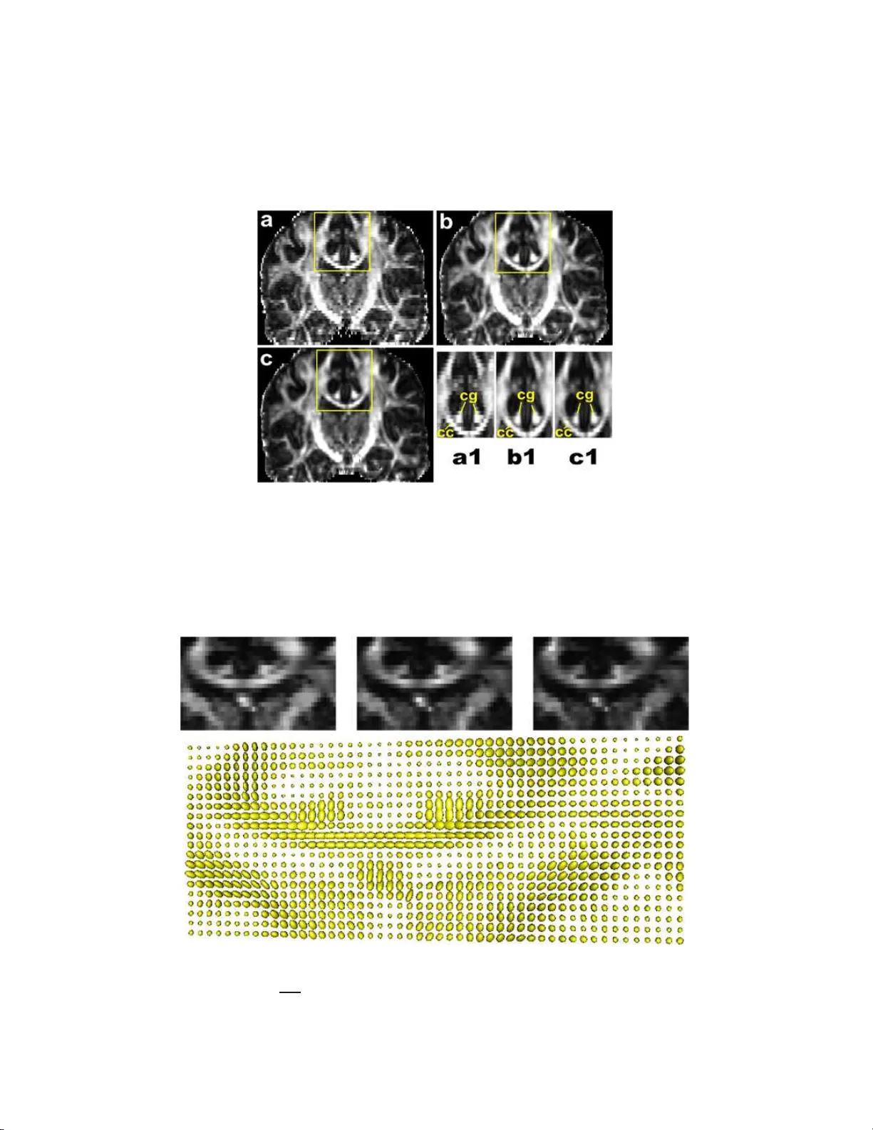
The Annals of Applie d Statistics 2009, V ol. 3, No. 3, 1102–1 123 DOI: 10.1214 /09-A OAS249 c  Institute of Mathematical Statistics , 2009 NON-EUCLIDEAN ST A TISTICS F OR COV ARIANCE MA TRICES, WITH APPLICA TIONS TO DIFFUSION TENS OR IMA GING 1 By Ian L. Dr yd e n, Alexey K oloydenko and Diwei Zhou University of South Car olina, R oyal Hol loway, University o f L ondon and University of Nottingham The statistical analysis of co v ariance matrix d ata is considered and, in particular, method ology is discussed whic h takes in to accoun t the non-Euclidean nature of the space of positive semi-definite sym- metric ma trices. The main motiv ation for the w ork is the analysis of diffusion tensors in medical image ana lysis. The primary fo cus is on estimation of a mean co v ariance matrix and , in particular, on the use of Pr ocru stes size-and-shap e s pace. Co mparisons are made with other estimation techniques, including using t h e matrix logarithm, matrix square root and Cholesky decomposition. Applications to diffusion tensor imaging are considered and, in particular, a new measure of fractional anisotrop y called Procrustes A nisotrop y is discussed. 1. In tro duction. The statistic al analysis of co v ariance matrices o ccurs in many imp ortant applicatio ns, for example, in d iffusion tensor imaging [Alexander ( 2005 ); Sc h w artzman, Dougherty and T a ylor ( 2008 )] or longitu- dinal data analysis [Daniels and Pourahmadi ( 20 02 )]. W e w ish to consider the situation where the data at h and are sample co v ariance matrice s, and w e w ish to estimate the p opulation co v ariance matrix and carry out statisti- cal inference. An example applicatio n is in diffusion tensor imaging where a diffusion tensor is a co v ariance matrix related to the molecular d isplacemen t at a particular v o xel in the brain, as described in S ection 2 . If a sample of co v ariance matrices is a v ailable, w e wish to estimate an a vera ge co v ariance matrix, or we ma y wish to inte rp olate in space b et w een t wo or more estimated cov ariance matrices, or we may w ish to carry out tests for equalit y of mean co v ariance matrices in different group s. Received Ma y 2008; rev ised Marc h 2009. 1 Supp orted b y a Leverh ulme Researc h F ellows hip and a Marie Curie Researc h T raining a w ard. Key wor ds and phr ases. Anisotropy, Cholesky, geodesic, matrix logarithm, principal components, Pro crustes, R iemannian, shap e, size, Wishart. This is an electronic repr in t of the original article published b y the Institute of Mathematical Statistics in The Annals of Appl ie d Statistics , 2009, V ol. 3, No. 3 , 110 2–112 3 . This reprint differs from the orig inal in pag ination and typogr a phic detail. 1 2 I. L. D R Y DEN, A. K OLOYDENKO AND D. ZH OU The usual approac h to estimating mean co v ariance matrices in Statistics is to assume a scaled Wishart distribution for the data, and then the maximum lik eliho o d estimato r (m.l.e.) of the p opulation co v ariance matrix is the arith- metic mean of the s amp le co v ariance mat rices. The est imator can b e formu- lated as a least sq u ares estimator u sing Euclidean dista nce. Ho w ever, sin ce the space of p ositiv e semi-definite symmetric matrices is a non-Euclidean space, it is more n atural t o use alternativ e distances. In Section 3 w e define what is meant b y a mean co v ariance matrix in a non-Euclidean space, us- ing the F r´ ec het mean. W e then review some recen tly prop osed tec hniques based on matrix logarithms and also consider estimators based on matrix decomp ositions, s uc h as the Cholesky deco mp osition and the matrix square ro ot. In Section 4 w e int ro duce an alte rnativ e approac h to the statist ical anal- ysis of co v ariance matrices u sing the Kendall’s ( 1989 ) size -and-shap e space. Distances, minimal geodesics, sample F r ´ ec het means, tangent spaces and practical estimators based on Pr o crustes analysis are all discussed. W e in- v estigate prop erties of the est imators, including consistency . In Section 5 we compare th e v arious c hoices of m etrics and their prop- erties. W e in ve stigate measures of anisotrop y and discuss the deficien t ran k case in particular. W e consider the motiv ating applications in Section 6 where th e analysis of diffusion tensor images and a sim ulation study are in vestig ated. Finally , w e conclude with a br ief discuss ion. 2. Diffusion tensor imaging. In m edical image analysis a p articular t yp e of co v ariance matrix arises in diffusion w eigh ted imaging called a diffusion tensor. The diffusion tensor is a 3 × 3 co v ariance matrix whic h is estimated at eac h v oxe l in the brain, and is obtained b y fitti ng a physica lly-motiv ated mo del on measurements from the F ourier transform of the molecule displace- men t densit y [Ba sser, Mattiello and Le Bihan ( 1994 ); Alexander ( 2005 )]. In the diffu sion tensor mo del the wa ter molecules at a vo xel diffuse accord- ing to a multiv ariate n ormal model cen tered on the vo xel and with co v ari- ance matrix Σ. Th e d isplacemen t of a wate r molecule x ∈ R 3 has probabilit y densit y function f ( x ) = 1 (2 π ) 3 / 2 | Σ | 1 / 2 exp  − 1 2 x T Σ − 1 x  . The conv en tion is to call D = Σ / 2 the diffusion tensor, wh ic h is a s ymmetric p ositiv e se mi-definite matrix. The diffusion tensor is estimated at eac h vo xel in the image f r om the av ailable MR images. The MR scanner has a set of magnetic field gradien ts applied at directions g 1 , g 2 , . . . , g m ∈ RP 2 with scanner gradien t parameter b , w here RP 2 is the real pro jectiv e sp ace of axial directions (with g j ≡ − g j , k g j k = 1). The data at a vo xel consist of signals ( Z 0 , Z 1 , . . . , Z m ) whic h are related to the F ourier transf orm of the NON-EUCLIDEAN ST A TISTICS FOR COV ARIANCE MA TRICES 3 Fig. 1. Visualization of a diffusion tensor as an el lipsoid. The princip al axis i s also displaye d. displacemen ts in axial directi on g j ∈ RP 2 , j = 1 , . . . , m , and the reading Z 0 is obtained w ith no gradien t ( b = 0). The F ourier tr ans form in axial direction g ∈ RP 2 of the m u ltiv ariate Ga ussian displacemen t densit y is giv en b y F ( g ) = Z exp( i √ bg ) f ( x ) dx = exp( − bg T D g ) , and the theoretical mo del for the signals is Z j = Z 0 F ( g j ) = Z 0 exp( − bg T j D g j ) , j = 1 , . . . , m. There are a v ariet y of metho ds a v ailable for estimating D from the data ( Z 0 , Z 1 , . . . , Z m ) at eac h v o xel [see Alexander ( 2005 )], including least squares regression and Ba y esian estimation [e.g., Zhou et al. ( 2008 )]. Noise mo dels include log-Gaussian, Gaussian and , more r ecentl y , R ician noise [W ang et al. ( 2004 ); Fillard et al. ( 200 7 ); Basu, Fletc her and Whitak er ( 2006 )]. A common metho d for visualizing a diffusion tensor is an ellipsoid with principal axes giv en by the eig en vect ors of D , and lengths of axes prop ortional to √ λ i , i = 1 , 2 , 3 . An example is giv en in Figure 1 . If a sample of diffusion tensors is av ailable, we may w ish to e stimate an a vera ge diffusion tensor matrix, in v estigate the structure of v ariabilit y in diffusion tensors or in terp olate at higher spatial resolution b et ween t wo or more estimated diffusion tensor matrices. In diffusion tensor imaging a strongly anisotropic d iffusion tensor indicates a strong direction of white matter fib er tracts, and plots of measures of anisotrop y are ve ry useful to neurologists. A measure that is v ery commonly used in diffusion tensor imaging is F ractional Anistropy , F A = ( k k − 1 k X i =1 ( λ i − ¯ λ ) 2  k X i =1 λ 2 i ) 1 / 2 , where 0 ≤ F A ≤ 1 and λ i are t he eigen v alues of the diffusion tensor matrix. Note that F A ≈ 1 if λ 1 ≫ λ i ≈ 0 , i > 1 (v ery strong p rincipal axis) and F A = 0 for isotrop y . In diffusion tensor imaging k = 3 . 4 I. L. D R Y DEN, A. K OLOYDENKO AND D. ZH OU Fig. 2. A n F A map fr om a sl i c e in a human br ain. Lighter values i ndi c ate higher F A. In Figure 2 we see a plot of F A from an example health y h u man brain. W e fo cus on the small inset region in the b ox, and we w ould like to in terp olate the displa y ed imag e to a fin er scale. W e return to this application in Section 6.3 . 3. Co v ariance matrix estimat ion. 3.1. Euclide an distanc e. Let us consider n sample co v ariance matrices (symmetric and positiv e semi-definite k × k matrices) S 1 , . . . , S n whic h are our data (or sufficien t statist ics). W e assume that the S i are indep end en t and iden tically distributed (i.i.d.) from a distribution wit h mea n co v ariance matrix Σ, although we shall elaborate more lat er in S ection 3.2 about what is mean t b y a “mean co v ariance matrix.” T he m ain aim is to estimate Σ . More complicated mo deling scenarios are also of in terest, but for no w we just concen trate on estima ting the mean co v ariance matrix Σ . The most common appr oac h is to assume i.i.d. scaled Wishart distribu- tions for S i with E ( S i ) = Σ, and the m .l.e. for Σ is ˆ Σ E = 1 n P n i =1 S i . This estimator can also b e obtained if using a least squares app roac h b y min imiz- ing the sum of square Euclidean distances. The Euclidean distance b etw een t wo matrices is giv en b y d E ( S 1 , S 2 ) = k S 1 − S 2 k = q trace { ( S 1 − S 2 ) T ( S 1 − S 2 ) } , (1) where k X k = q trace( X T X ) is the Euclidean norm (al so known as th e F rob e- nius norm). The least squares estimator is giv en b y ˆ Σ E = arg inf Σ n X i =1 k S i − Σ k 2 . Ho wev er, the space of p ositiv e semi-definite s y m metric matrices is a n on- Euclidean space and other choic es of d istance are more natural. One par- ticular d ra w b ac k with Eu clidean distance is when extrapolating beyond the NON-EUCLIDEAN ST A TISTICS FOR COV ARIANCE MA TRICES 5 data, nonp ositiv e semi-definite estimate s can b e obtained. There are other dra wbac ks when int erp olating co v ariance matrices, as we shall see in our applications in Section 6 . 3.2. The F r´ echet me an. When using a non-Euclidean distance d ( · ) we m u st define w hat is mean t b y a “mean co v ariance matrix.” Consider a prob- abilit y distribution for a k × k co v ariance mat rix S o n a Riemannian metric space with densit y f ( S ). The F r ´ ec het ( 1948 ) mean Σ is defined as Σ = arg inf Σ 1 2 Z d ( S, Σ ) 2 f ( S ) dS, and is also kno wn as the Karc her mean [Karc her ( 1977 )]. The F r ´ ec het mean need not b e unique in general, although for man y distributions it will b e. Pro vid ed the distribu tion is su pp orted only on the geo desic ball of radiu s r , suc h that the geod esic ball of radius 2 r is r egular [i.e., suprem um of sectional curv atures is less than ( π/ (2 r )) 2 ], then the F r ´ ec het mean Σ is un ique [Le ( 1995 )]. The sup p ort to ensure uniqueness can b e v ery large. F or example, for Euclidean spaces (with sectional curv ature zero), or f or non-Eu clidean spaces with negativ e sectional curv ature, the F r ´ ec het mean is alw a ys u nique. If we ha ve a sample S 1 , . . . , S n of i.i.d. observ ations av ailable, then the sample F r ´ ec het mean is calculate d b y findin g ˆ Σ = arg inf Σ n X i =1 d ( S i , Σ) 2 . Uniqueness of the samp le F r ´ ec het mean can also b e determined from the result of Le ( 1995 ). 3.3. Non-Euclide an c ovarianc e estimator s. A recen tly deriv ed approac h to co v ariance matrix estimation is to use matrix logarithms. W e wr ite the logarithm of a p ositiv e definite cov ariance matrix S as follo ws. Let S = U Λ U T b e the u sual sp ectral decomp ositio n, with U ∈ O ( k ) an orthogonal matrix and Λ diagonal with strictly p ositiv e ent ries. Let log Λ b e a d iagonal matrix with logarithm of the diagonal element s of Λ on the diagonal. The logarithm of S is gi v en by log S = U (log Λ) U T and lik ewise the exp onen tial of the m atrix S is exp S = U (exp Λ) U T . Arsign y et al. ( 2007 ) p r op ose the use of the log-Euclidea n distance, where Euclidean distance b etw een the logarithm of co v ariance matric es is used for statistical analysis, that is, d L ( S 1 , S 2 ) = k log ( S 1 ) − log( S 2 ) k . (2) An estimator for the mean p opulation co v ariance matrix using this ap- proac h is g iv en b y ˆ Σ L = exp ( arg inf Σ n X i =1 k log S i − log Σ k 2 ) = exp ( 1 n n X i =1 log S i ) . 6 I. L. D R Y DEN, A. K OLOYDENKO AND D. ZH OU Using this metric av oids extrap olation p roblems into matrices with nega- tiv e eige n v alues, but it cannot deal with p ositiv e semi-definite matrices of deficien t rank. A fur ther logarithm-based estimator uses a Riemannian m etric in the space of square symmetric p ositiv e definite matrices d R ( S 1 , S 2 ) = k log ( S − 1 / 2 1 S 2 S − 1 / 2 1 ) k . (3) The estimator (sample F r ´ ec het mean) is giv en b y ˆ Σ R = arg inf Σ n X i =1 k log( S − 1 / 2 i Σ S − 1 / 2 i ) k 2 , whic h has b een explored by Pe nnec, Fillard and Ay ac he ( 2006 ), Moakher ( 2005 ), Sch w artzman ( 2006 ), Lenglet, Rousson and Deric he ( 2006 ) and Fletc her and Joshi ( 2007 ). T he estimate can b e obtained using a gradi- en t descen t a lgorithm [e .g., see P enn ec ( 1999 ); P ennec, Filla rd and Aya c he ( 2006 )]. Note that th is Riemannian metric space has neg ativ e sectional c ur- v ature a nd so the p opulation and sample F r´ ec het means are unique in this case. Alternativ ely , one can u s e a reparamete rization of the co v ariance matrix, suc h as the Cholesky decomp osition [W ang et al. ( 2004 )], w here S i = L i L T i and L i = chol( S i ) is lo wer triangular with p ositiv e d iagonal en tries. Th e Cholesky distance is giv en b y d C ( S 1 , S 2 ) = k chol( S 1 ) − c hol ( S 2 ) k . (4) A least squares estimator can b e obtained from ˆ Σ C = ˆ ∆ C ˆ ∆ T C , where ˆ ∆ C = arg inf ∆ ( 1 n n X i =1 k L i − ∆ k 2 ) = 1 n n X i =1 L i . An equiv alen t mo del-based approac h wo uld use an in dep endent Gaussian p erturb ation mo del for the lo w er triangular part of L i , with mean giv en by the lo we r triangular part of ∆ C , and so ˆ ∆ C is the m.l.e. of ∆ C under this mo del. Hence, in this approac h the av eraging is carried out on a squ are ro ot t yp e-scale , whic h wo uld indeed b e the case for k = 1 dimensional case where the estimat e of v ariance w ould b e the square of the mean of the samp le standard deviations. An alternativ e d ecomp osition is the matrix square ro ot where S 1 / 2 = U Λ 1 / 2 U T , whic h has not b een used in this con text b efore as far as w e are a ware. The distance is giv en b y d H ( S 1 , S 2 ) = k S 1 / 2 1 − S 1 / 2 2 k . (5) NON-EUCLIDEAN ST A TISTICS FOR COV ARIANCE MA TRICES 7 A least squares estimator can b e obtained from ˆ Σ H = ˆ ∆ H ˆ ∆ T H , where ˆ ∆ H = arg inf ∆ ( n X i =1 k S 1 / 2 i − ∆ k 2 ) = 1 n n X i =1 S 1 / 2 i . Ho wev er, b ecause L i RR T L T i = L i L T i for R ∈ O ( k ) , another new alterna- tiv e is to relax the lo we r triangular or s qu are ro ot parameterizatio ns and matc h the initial decomp ositions closer in terms of Euclidean distance b y optimizing ov er rotati ons and reflections. T his id ea provi des the rational e for the main approac hes in this pap er. 4. Pro crustes size-and-shap e analysis. 4.1. Non-Euclide an size-and-shap e metric. The non-Euclidean size-and- shap e metric b et we en tw o k × k co v ariance matrices S 1 and S 2 is defined as d S ( S 1 , S 2 ) = inf R ∈ O ( k ) k L 1 − L 2 R k , (6) where L i is a decomp osition of S i suc h that S i = L i L T i , i = 1 , 2. F or example, w e could ha v e th e Cholesky decomp osition L i = chol( S i ) , i = 1 , 2 , whic h is lo wer triangular with p ositiv e diagonal elemen ts, or we could consider the matrix square ro ot L = S 1 / 2 = U Λ 1 / 2 U T , where S = U Λ U T is the sp ectral decomp osition. Note that S 1 = ( L 1 R )( L 1 R ) T for an y R ∈ O ( k ), and so the distance in vo lv es matc hing L 1 optimally , in a least- squares sense, to L 2 b y rotation and reflectio n. Since S = LL T , then the decomp osition is repr e- sen ted b y an equiv alence class { LR : R ∈ O ( k ) } . F or practical computation w e often need t o c ho ose a r epresen tativ e from this class, called an i con, and in our computations w e shall c h o ose the Cholesky decomp osition. The Pro crustes solution for matc hin g L 2 to L 1 is ˆ R = arg in f R ∈ O ( k ) k L 1 − L 2 R k (7) = U W T , where L T 1 L 2 = W Λ U T , U, W ∈ O ( k ) , and Λ is a diagonal matrix of p ositiv e singular v alues [e.g., see Mardia, Ken t and Bibb y ( 1979 ), page 416]. This metric h as b een used p r eviously in the analysis of p oin t set configur a- tions where inv ariance u nder translation, rotation and reflection is required . Size-and-shap e s p aces w ere in tro d uced by Le ( 1988 ) and Kendall ( 198 9 ) as part of the p ioneering w ork on the shap e analysis of landmark data [cf. Kendall ( 1984 )]. The deta iled ge ometry of these spaces is give n b y Kendall et al. [( 1999 ), pages 254–264] , and, in particular, the size-and-shap e space is a cone with a w arp ed-pro duct met ric and has p ositiv e sectional curv ature. 8 I. L. D R Y DEN, A. K OLOYDENKO AND D. ZH OU Equation ( 6 ) is a Riemannian metric in the reflection size-and-shap e space of ( k + 1)-p oints in k dimensions [Dryden and Mardia ( 1998 ), Ch apter 8]. In particular, d S ( · ) is the reflection size-and-shap e distance b et we en the ( k + 1) × k configurations H T L 1 and H T L 2 , wh ere H is the k × ( k + 1) Helmert sub-matrix [Dryden and Mardia ( 1 998 ), page 34] whic h has j th ro w giv en by ( h j , . . . , h j | {z } j times , − j h j , 0 , . . . , 0 | {z } k − j times ) , h j = −{ j ( j + 1) } − 1 / 2 , for j = 1 , . . . , k . Hence, the statistic al analysis of co v ariance matrices can b e considered equiv alen t to the dual problem of anal yzing reflection size-and-shap es. 4.2. Minimal ge o desic and tangent sp ac e. Let us consider the minimal geod esic path through the reflection size-and-shap es of L 1 and L 2 in the reflection size-and-shap e space, where L i L T i = S i , i = 1 , 2. F ollo wing an ar- gumen t s imilar to that for the minimal geo desics in sh ap e spaces [Kend all et al. ( 1999 )], th is minimal geo desic ca n b e isometrically expressed as L 1 + tT , where T are the horizon tal tangen t co-ordinates of L 2 with p ole L 1 . Kendall et al. [( 1999 ), Section 11.2] discuss size-a nd-shap e spaces without reflect ion in v ariance, how ev er, the r esults with reflection in v ariance are similar, as re- flection do es not c h ange the lo cal geometry . The horizon tal tangen t co ordinates satisfy L 1 T T = T L T 1 [Kendall et al. ( 1999 ), page 258]. Explicitly , the h orizon tal tangen t coordinates are giv en b y T = L 2 ˆ R − L 1 , ˆ R = i nf R ∈ O ( k ) k L 1 − L 2 R k , where ˆ R is the Pro crustes matc h of L 2 on to L 1 giv en in ( 7 ). So, the geod esic path starting at L 1 and ending at L 2 is giv en b y w 1 L 1 + w 2 L 2 ˆ R, where w 1 + w 2 = 1 , w i ≥ 0 , i = 1 , 2, and ˆ R is giv en in ( 7 ). Minimal geo desics are useful in applications for in terp olati ng b et wee n tw o co v ariance mat rices, in regression mod eling of a series o f co v ariance matrices, and for extrap ola- tion and prediction. T angen t spaces are very useful in practica l applications, where one uses Euclidean distances in the tangen t space as appro ximations to the non- Euclidean metrics in the size- and-shap e space itself. Suc h constructio ns are useful for appro ximate m ultiv ariate n ormal based inference, d imension r e- duction u s ing pr in cipal comp onen ts analysis and large sample asymptotic distributions. NON-EUCLIDEAN ST A TISTICS FOR COV ARIANCE MA TRICES 9 4.3. Pr o crustes me an c ovarianc e matrix. Let S 1 , . . . , S n b e a sample of n p ositiv e semi-definite co v ariance matrices eac h of size k × k from a dis- tribution with densit y f ( S ), and w e w ork with the Pro crustes metric ( 6 ) in order to estimate th e F r´ ec het mean co v ariance matrix Σ. W e assu me that f ( S ) leads to a unique F r ´ ec het mean (se e Section 3.2 ). The sample F r ´ ec het mean is calc ulated b y find in g ˆ Σ S = arg inf Σ n X i =1 d S ( S i , Σ) 2 . In the dual size-and-shap e formula tion w e can write this as ˆ Σ S = ˆ ∆ S ˆ ∆ T S , where ˆ ∆ S = arg inf ∆ n X i =1 inf R i ∈ O ( k ) k H T L i R i − H T ∆ k 2 . (8) The solution can b e foun d using the Generalized Pro crustes Algo rithm [Go we r ( 19 75 ); Dryden and Mardia ( 1998 ), page 90], wh ic h is a v ailable in the sh apes library (written by the first author of this pap er) in R [R De- v elopment Core T eam ( 200 7 )]. Note that if the data lie within a geodesic ball of radius r suc h that the ge o desic ball of radius 2 r is regular [Le ( 1995 ); Kendall ( 1990 )], th en the algorithm fi nds the global un ique minim u m solu- tion to ( 8 ). Th is condition can be c hec ke d for an y dataset and , in pr actic e, the algorithm w orks v ery w ell indeed. 4.4. T angent sp ac e infer enc e. If the v ariabilit y in the data is not to o large, then w e can pro ject the data in to the tangen t space and carry out the usual Euclidean based inference in that space. Consider a sample S 1 , . . . , S n of co v ariance matrice s with s ample F r ´ ec het mean ˆ Σ S and tangen t space coordinates with p ole ˆ Σ S = ˆ ∆ S ˆ ∆ T S giv en by V i = ˆ ∆ S − L i ˆ R i , where ˆ R i is the Pro cru stes rotati on for matc hing L i to ˆ ∆ S , i = 1 , . . . , n, and S i = L i L T i , i = 1 , 2. F requen tly one wishes to reduce t he dimension of the problem, for exam- ple, using principal comp onent s analysis. Let S v = 1 n n X i =1 v ec ( V i ) v ec ( V i ) T , where v ec is the vect orize op eratio n. The pr incipal comp onen t (PC) load- ings are giv en b y ˆ γ j , j = 1 , . . . , p , the eigen v ectors of S v corresp onding to the eigen v alues ˆ λ 1 ≥ ˆ λ 2 ≥ · · · ≥ ˆ λ p > 0, where p is the num b er of nonzero eigen v alues. The PC s core for the i th ind ividual on PC j is giv en b y s ij = ˆ γ T j v ec ( V i ) , i = 1 , . . . , n, j = 1 , . . . , p. 10 I. L. D R Y DEN, A. K OLOYDENKO AND D. ZH OU In general, p = min( n − 1 , k ( k + 1) / 2). The effect of the j th PC can b e examined by ev aluating Σ( c ) = ( ˆ ∆ S + c vec − 1 k ( ˆ λ 1 / 2 j ˆ γ j ))( ˆ ∆ S + c vec − 1 k ( ˆ λ 1 / 2 j ˆ γ j )) T for v arious c [often in the range c ∈ ( − 3 , 3), for example] , where v ec − 1 k (v ec( V )) = V f or a k × k mat rix V . T angen t space inference ca n pro ceed o n the first p PC sco res, or possibly in lo wer dimensions if desired. F or example, Hotelling’ s T 2 test can b e carried out to examine group differences, or regression mo dels could b e deve lop ed for inv estigat ing the PC s cores as resp onses v ersu s v arious co v ariates. W e shall consider p rincipal comp onents analysis of co v ariance matrice s in an application in Section 6.2 . 4.5. Consistency. Le ( 1995 , 2001 ) and Bhattac hary a and Patrange naru ( 2003 , 2005 ) p ro vid e consistency results for Riemannian manifolds, which can b e applied d irectly to our situation. Consider a distribution F on the space of co v ariance matrices whic h has size-and-shap e F r ´ ec het mean Σ S . Let S 1 , . . . , S n b e i.i.d. from F , suc h that they lie within a geo desic ball B r suc h that B 2 r is regular. Then ˆ Σ S P → Σ S , as n → ∞ , where Σ S is un ique. In addition, w e can deriv e a central limit th eorem result as in Bh attac h ary a and P atrangenaru ( 2005 ), where the tangen t co ord inates ha ve an app ro ximate multi v ariate normal d istribution for large n . Hence, confidence r egions b ased on the b o otstrap can b e obtained, as in Amaral, Dryden and W oo d ( 2007 ) and Bhattac hary a and Pa trangenaru ( 2003 , 2005 ). 4.6. Sc ale invarianc e. In some applications it may b e of in terest to con- sider inv ariance ov er isotropic sca ling of the co v ariance matrix. In this case w e could consider the represen tation of the co v ariance matrix using Kendall’s reflection shap e space, with the shap e m etric give n b y the full P r o crustes distance d F ( S 1 , S 2 ) = inf R ∈ O ( k ) ,β > 0     L 1 k L 1 k − β L 2 R     , (9) where S i = L i L T i , i = 1 , 2, and β > 0 is a scale parameter. Another choic e of the estimated co v ariance matrix from a sample S 1 , . . . , S n , whic h is scale in v ariant and based on the full Pro crustes mean shap e (extrinsic mean), is ˆ Σ F = ˆ ∆ F ˆ ∆ T F , where ˆ ∆ F = arg inf ∆ n X i =1 n inf R i ∈ O ( k ) , β i > 0 k β i L i R i − ∆ k 2 o , NON-EUCLIDEAN ST A TISTICS FOR COV ARIANCE MA TRICES 11 T able 1 Notation and defin itions of the distanc es an d estimators Name Notation F orm Estimator Equation Euclidean d E ( S 1 , S 2 ) k S 1 − S 2 k ˆ Σ E ( 1 ) Log-Euclidean d L ( S 1 , S 2 ) k log( S 1 ) − log ( S 2 ) k ˆ Σ L ( 2 ) Riemannian d R ( S 1 , S 2 ) k log( S − 1 / 2 1 S 2 S − 1 / 2 1 ) k ˆ Σ R ( 3 ) Cholesky d C ( S 1 , S 2 ) k chol ( S 1 ) − chol( S 2 ) k ˆ Σ C ( 4 ) Root Euclidean d H ( S 1 , S 2 ) k S 1 / 2 1 − S 1 / 2 2 k ˆ Σ H ( 5 ) Procrustes size-and-shap e d S ( S 1 , S 2 ) inf R ∈ O ( k ) k L 1 − L 2 R k ˆ Σ S ( 6 ) F ull Pro crustes shape d F ( S 1 , S 2 ) inf R ∈ O ( k ) ,β > 0 k L 1 k L 1 k − β L 2 R k ˆ Σ F ( 9 ) P o w er Euclidean d A ( S 1 , S 2 ) 1 α k S α 1 − S α 2 k ˆ Σ A ( 10 ) and S i = L i L T i , i = 1 , . . . , n , and β i > 0 are scale parameters. Th e solutio n can again b e found from the Generalized Pro crus tes Algorithm u sin g the sha pes library in R. T angen t space inference can then pro ceed in an analogous manner to that of Section 4.4 . 5. Comparison of approac h es. 5.1. Choic e of metrics. In applications there are sev eral c hoices of dis- tances b et wee n co v ariance matrices that one could consider. F or complete- ness w e list the metrics and the e stimators considered in this pap er in T able 1 , and w e discuss briefly some of their prop erties. Estimators ˆ Σ E , ˆ Σ C , ˆ Σ H , ˆ Σ L , ˆ Σ A are straightfo rwa rd to compute using arith- metic a v erages. Th e Pro crustes b ased estimators ˆ Σ S , ˆ Σ F in volv e the use of the Generaliz ed Pr o crustes Algorithm, wh ich works very wel l in practice . The Riemannian metric estimator ˆ Σ R uses a gradient descen t algorithm whic h is guarant eed to con v erge [see P enn ec ( 1999 ); P enn ec, Fillard and Ay ac he ( 20 06 )]. All these distances except d C are in v arian t und er simult aneous r otatio n and reflection of S 1 and S 2 , that is, the distances are un changed by replacing b oth S i b y V S i V T , V ∈ O ( k ) , i = 1 , 2. Metrics d L ( · ) , d R ( · ) , d F ( · ) are in v ari- an t under sim ultaneous scaling of S i , i = 1 , 2 , that is, replacing b oth S i b y β S i , β > 0 . Metric d R ( · ) is also affine in v arian t, that is, the distances are unc hanged by replacing b oth S i b y AS i A T , i = 1 , 2 , where A is a general k × k full rank matrix. Metrics d L ( · ) , d R ( · ) h a ve the prop ert y that d ( A, I k ) = d ( A − 1 , I k ) , where I k is the k × k iden tity matrix. Metrics d L ( · ) , d R ( · ) , d F ( · ) are not v alid for comparin g rank deficient co- v ariance mat rices. Finally , there are problems with extrapolation with met- ric d E ( · ): ext rap olate to o far and the matrices are no longer positiv e semi- definite. 12 I. L. D R Y DEN, A. K OLOYDENKO AND D. ZH OU 5.2. Anisotr opy. In some applications a measure of anisotropy of th e co v ariance matrix ma y b e required, and in Section 2 w e describ ed the com- monly used F A measure. An alternativ e is to use the fu ll Pro cru stes shap e distance to isotrop y and w e ha v e P A = s k k − 1 d F ( I k , S ) = s k k − 1 inf R ∈ O ( k ) ,β ∈ R +     I k √ k − β chol( S ) R     , = ( k k − 1 k X i =1 ( √ λ i − √ λ ) 2  k X i =1 λ i ) 1 / 2 , where √ λ = 1 k P √ λ i . Note that th e maximal v alue of d F distance fr om isotrop y to the rank 1 co v ariance matrix is p ( k − 1) /k , whic h follo w s from Le ( 1992 ). W e includ e th e scale factor when defining the Pro crustes Anisotrop y (P A), and so 0 ≤ P A ≤ 1, with P A = 0 in dicating iso trop y , and P A ≈ 1 indi- cating a v ery strong principal axis. A final measure based on metrics d L or d R is the geod esic anisotrop y GA = ( k X i =1 (log λ i − log λ ) 2 ) 1 / 2 , where 0 ≤ GA < ∞ [Arsign y e t al. ( 2007 ); Fillard et a l. ( 2007 ); Fletc her and Joshi ( 2007 )], which has b een u sed in diffu sion tensor analysis in medical imaging with k = 3. 5.3. Deficient r ank c ase. In some applications co v ariance matrices are close to b eing deficien t in rank. F or example, when F A or P A are equal to 1, then the co v ariance matrix is of rank 1 . The Pr o crustes metrics can easily deal with deficien t rank matrices, wh ic h is a strong adv anta ge of the approac h. Ind eed, Kend all’s ( 1984 , 19 89 ) original m otiv ation for dev eloping his theory of shap e wa s to in ve stigate rank 1 configurations in the con text of detecting “flat” (collinea r) triangle s in arc heology . The use of ˆ Σ L and ˆ Σ R has strong connections with the use of Bo okstein’s ( 1986 ) hyperb olic shap e space and Le and Sm all’s ( 1999 ) simplex shap e space, and suc h spaces cannot deal with deficien t rank configurations. The us e of th e Cholesky decomp osition has strong connections with Bo ok- stein coordin ates and Go o dall–Mardia coordinates in shap e analysis, w h ere one registers configurations on a common baseline [Bookstein ( 1986 ); Goo d all and Mardia ( 1992 )]. F or small v ariabilit y the b aseline registration m etho d and Pro crustes su p erimp ositio n tec h niques are similar, and there is an ap- pro ximate li near relati onship b et ween the t wo [Ke n t ( 1 994 )]. In shap e anal- ysis edge sup erimp osition tec hn iqu es can b e v ery un reliable if th e baseline is v ery small in length, whic h would corresp ond to v ery small v ariabilit y in NON-EUCLIDEAN ST A TISTICS FOR COV ARIANCE MA TRICES 13 Fig. 3. F our differ ent ge o desic p aths b etwe en the two tensors. The ge o desic p aths ar e obtaine d us ing d E ( · ) (1s t r ow), d L ( · ) (2nd r ow), d C ( · ) (3r d r ow) and d S ( · ) (4th r ow). particular diagonal elemen ts of the co v ariance matrix in the curren t con text. Cholesky metho ds w ould b e u nreliable in such ca ses. Also, Bookstein co or- dinates induce correlations in the s hap e v ariables and, hence, estimation of co v ariance structur e is b iased [Ken t ( 1994 )]. Hence, in general, P r o crustes tec hniques are p referred ov er edge su p erimp osition tec h niques in shap e anal- ysis. Hence , this would mean i n the current con text that the Pro crustes ap- proac hes of this pap er should b e preferred to inference u s ing th e Ch olesky decomp osition. 6. Applications. 6.1. Interp olatio n of c ovarianc e ma tric es. F requen tly in d iffusion tensor imaging one w ish es to carry out in terp olatio n b et wee n tensors. When the tensors are quite differen t, in terp olation using different metrics can lead to v ery different results. F or example, consider Figure 3 , where four different geod esic paths are plotted b et ween t w o tensors. Arsign y et al. ( 2007 ) note that the Euclidean metric is prone to sw elling, which is seen in this example. Also, the log-Euclidean met ric giv es strong weig h t to small v olumes. In th is example the Ch olesky and Pro crustes size-and-shap e paths lo ok rather dif- feren t, d u e to the extra rotation in the Pro crustes m etho d . F rom a v ariet y of examples it do es seem cle ar that the Euclidean metric is v ery problematic, esp ecially d ue to the sw elling of the v olume. In general, the log-Euclidean and Pro crustes size-and-shap e metho ds seem pr eferable. In some applicat ions, for example, fib er trac kin g, w e ma y n eed to in ter- p olate b et wee n sev eral cov ariance matrices on a grid, in whic h case we can use w eigh ted F r´ ec h et m eans ˆ Σ = arg inf Σ n X i =1 w i d ( S i , Σ) 2 , n X i =1 w i = 1 , 14 I. L. D R Y DEN, A. K OLOYDENKO AND D. ZH OU Fig. 4 . Demons tr ation of PCA for c ovarianc e matric es. The t rue ge o desic p ath is given in the p enultimate r ow (black). We then add noi se in the thr e e ini tial r ows (r e d). Then we estimate the me an and find the first princip al c omp onent (yel low), displaye d in the b ottom r ow. where th e wei gh ts w i are prop ortional to a function of the distance (e.g., in verse distance or Kriging based we igh ts). 6.2. Princip al c omp onents analysis of diffusion tensors. W e consider now an example estimating the pr incipal geo desics of the co v ariance matrices S 1 , . . . , S n using the Pro crustes size-and-shap e metric. Th e data are dis- pla yed in Figure 4 and h ere k = 3. W e consider a true geodesic path (blac k) and ev aluate 11 equ ally spaced co v ariance matrices along this path. W e then ad d noise for three separate realizati ons of noisy paths (in red). T he noise is indep endent and identic ally d istributed Gaussian and is added in the du al space o f th e tangen t coordinates. First, the o v erall Pro crustes size- and-shap e mean ˆ Σ S is computed based on all the data ( n = 33), and then the Procrus tes size-a nd-shap e tangen t space co- ordinates are obtained. The first pr incipal comp onent loadings are computed and pr o jected back to giv e an esti mated minimal geo desic in the co v ariance matrix space. W e plot this path in y ello w b y displa ying 11 co v ariance matrices along the path. As we w ould exp ect, the first prin cipal component path b ears a strong similarit y to th e true geo desic path. The p ercent ages of v ariabilit y explained by the first three PCs are as follo ws: PC1 (72. 0%), PC2 (8.8%), PC 3 (6.5%). The data can also b e seen in the dual Pro crustes space of 4 p oint s in k = 3 dimensions in Figure 5 . W e also see the data after applying the Procru s tes fitting, w e sho w the effects of the fi rst three pr in cipal comp onen ts, and al so the plot of the first three PC scores. NON-EUCLIDEAN ST A TISTICS FOR COV ARIANCE MA TRICES 15 Fig. 5 . (top left) The no isy c onfigur ations in the dual sp ac e of k + 1 = 4 p oints in k = 3 dimensions. F or e ach c onfigur ation p oint 1 is c olor e d black, p oint 2 i s r e d, p oint 3 is gr e en and p oint 4 is blue, and the p oints in a c onfigur ation ar e joine d by lines. (top right ) The Pr o crustes r e gister e d data, after r emoving tr anslation, r otation and r efle ction. (b ottom left) The Pr o crustes me an size-and-sh ap e, with ve ctors dr awn along the dir e ctions of the first thr e e PCs (PC1—black, PC2—r e d, PC3—gr e en). (b ottom right) The first thr e e PC sc or es. The p oints ar e c olor e d by the p osition along the true ge o desic fr om left to right (black, r e d, gr e en, blue, cyan, purple, yel low, gr ey, black, r e d, gr e en). 6.3. Interp olatio n. W e consider the int erp olation of part of the brain image in Figure 2 . In Figure 6 (a) w e see the original F A image, and in Figure 6 (b) and (c) we see in terp olated images u sing size-and-shap e distance. The in terp olatio n is carried out at tw o equally spaced p oin ts b et ween v o xels, and Figure 6 (b) shows the F A image from th e inte rp olation and Figure 6 (c) sho w s the P A image. In the b otto m right plot of Figure 6 we highligh t the sele cted regions in the b o x. It is clear that the int erp olated images are smo other, and it is clear from the anisotropy maps of the in terp olated data that the cingulum (cg) is distinct from the corpus callosum (cc). 6.4. Anisotr opy. As a final ap p licatio n we consider some diffusion ten- sors ob tained from diffusion w eigh ted images in the brain. In Figure 7 w e see a coronal slice from the brain w ith the 3 × 3 tensors displa y ed. This image is a c oronal vie w of the b rain, and the corpus cal losum and cingulum can b e seen. The diagonal tract on the lo wer left is the an terior lim b of the 16 I. L. D R Y DEN, A. K OLOYDENKO AND D. ZH OU Fig. 6. F A maps fr om the original (a) and interp olate d (b) data. In (c) the P A map is displaye d, and i n (a1) , (b1) , (c1) we se e the zo ome d in r e gions marke d in (a) , (b) , (c) r esp e ctively. in tern al capsule and on the lo w er righ t w e see the sup erior fronto -o ccipital fasciculus. Fig. 7. In the upp er plots we se e the anisotr opy me asur es (left) F A, (midd le) P A, (right) GA. In the lower plot we se e the diffusion tenso rs, which have b e en sc ale d to have volume pr op ortional to √ F A . NON-EUCLIDEAN ST A TISTICS FOR COV ARIANCE MA TRICES 17 A t first sigh t all three measures app ear broadly similar. Ho w eve r, the P A image offers more con trast than the F A image in the highly a nisotropic region—the corpus callosum. Also, the GA ima ge has rather few er brighte r areas than P A or F A. Due to the imp ro ved contrast, w e b eliev e P A is sligh tly preferable in this example. 6.5. Simulation study. Finally , we consider a simulatio n study to com- pare the different estimators. W e consider the pr oblem of estimating a p op- ulation co v ariance matrix Ω from a random sample of k × k co v ariance ma- trices S 1 , . . . , S n . W e consider a random samp le generat ed as follo ws. Let ∆ = chol(Ω) and X i b e a random matrix with i.i.d. entries with E [( X i ) j l ] = 0 , v ar(( X i ) j l ) = σ 2 , i = 1 , . . . , n ; j = 1 , . . . , k ; l = 1 , . . . , k . W e tak e S i = (∆ + X i )(∆ + X i ) T , i = 1 , . . . , n. W e shall consider four error mo dels: I. Gaussian s qu are root: ( X i ) j l are i.i.d. N (0 , σ 2 ) for j = 1 , . . . , k ; l = 1 , . . . , k . I I. Gaussian Ch olesky: ( X i ) j l are i.i.d. N (0 , σ 2 ) for j ≤ k and zero other- wise. I I I. Log-Gaussian: i.i.d. Gaussian errors N (0 , σ 2 ) are add ed to the matrix logarithm of ∆ to giv e Y , and then the matrix exp onen tial of Y Y T is tak en. IV. Student’s t with 3 degrees of freedom: ( X i ) j l are i.i.d. ( σ / √ 3) t 3 for j = 1 , . . . , k ; l = 1 , . . . , k . W e consider the p erformance in a sim u lation study , with 1000 Mont e Carlo simulatio ns. The results are p r esen ted in T ables 2 and 3 for t w o choi ces of p opulation co v ariance matrix. W e took k = 3 and n = 10 , 30. In order t o in vestig ate the efficiency of the estimators, we u se three measures: estimate d mean square err or b et w een the estimate and the matrix Ω with metrics d E ( · ) , d S ( · ) and the estimated risk fr om us in g Stein loss [James and S tein ( 1961 )] whic h is giv en b y L ( S 1 , S 2 ) = trace( S 1 S − 1 2 ) − log det( S 1 S − 1 2 ) − k , where d et( · ) is the d eterminan t. Clearly the efficiency of the metho ds de- p ends strongly on the Ω a nd the error distribution. Consider the fi rst case where the mean has λ 1 = 1 , λ 2 = 0 . 3 , λ 3 = 0 . 1 in T able 2 . W e discuss mo del I fir st where the err ors are Gaussian on the matrix square ro ot scale. Th e efficiency is fairly similar for eac h estimator for n = 10, w ith ˆ Σ H p erforming the b est. F or n = 30 either ˆ Σ H or ˆ Σ S are b etter, with ˆ Σ E p erforming least w ell. F or mo del I I with Gaussian errors added in the Cholesky deco mp osition w e see that ˆ Σ C is the b est, although the other estimators are qu ite similar, with the exception of ˆ Σ E whic h is 18 I. L. D R Y DEN, A. K OLOYDENKO AND D. ZH OU w orse. F o r mo del II I with Gaussian errors on the m atrix logarithm scale all estimators are quite similar, as the v ariabilit y is rather small. The estimate ˆ Σ R is sligh tly b etter here than the others. F or m o del IV with Studen t’s t 3 errors we see that ˆ Σ H and ˆ Σ S are sligh tly b etter on the whole, although ˆ Σ E is again the wo rst p erformer. T able 2 Me asur es of efficiency, with k = 3 and σ = 0 . 1 . RMSE is the r o ot me an squar e err or using either the Euclide an norm or the Pr o crustes size-and-s hap e norm, and “St ein ” r efers t o the risk using the Ste in loss function. The smal lest value in e ach r ow is highlighte d i n b old. The me an has p ar ameters λ 1 = 1 , λ 2 = 0 . 3 , λ 3 = 0 . 1 . The err or distributions for Mo dels I–IV ar e Gaussian (squa r e r o ot), Ga ussian ( Cholesky), lo g-Gaussian and Stud ent’s t 3 , r esp e ctively ˆ Σ E ˆ Σ C ˆ Σ S ˆ Σ H ˆ Σ L ˆ Σ R ˆ Σ F I n = 10 RMSE( d E ) 0 .1136 0. 1057 0.1 04 0.1025 0.104 0.1176 0.1058 RMSE( d S ) 0.0911 0.082 0 .0802 0.0794 0.0851 0.0892 0.0813 Stein 0.0869 0.0639 0.0615 0.0604 0.0793 0.0728 0.0626 n = 30 RMSE( d E ) 0.0788 0.0669 0.0626 0.0611 0.0642 0.0882 0.0652 RMSE( d S ) 0.0691 0.0516 0.0475 0.0477 0.0525 0.0607 0.049 Stein 0.058 0. 0242 0.0207 0.0223 0.0295 0.0265 0.0216 I I n = 10 RMSE( d E ) 0.0973 0.0889 0.0911 0.0906 0.093 0.1014 0.0923 RMSE( d S ) 0.0797 0.0695 0.0714 0.0713 0.0752 0.0785 0.0721 Stein 0.07 0.0468 0.0499 0.0502 0.0573 0.0554 0.0506 n = 30 RMSE( d E ) 0.0641 0.0513 0.0535 0.0533 0.058 0.0732 0.0551 RMSE( d S ) 0.0585 0.0399 0.0422 0.0432 0.0471 0.0533 0.0431 Stein 0.0452 0.0151 0.0176 0.0196 0.0214 0.0214 0.0183 I I I n = 10 RMSE( d E ) 0.0338 0.0333 0.0336 0.0335 0.0333 0.0331 0.0336 RMSE( d S ) 0.0195 0.0193 0.0194 0.0194 0.0192 0.0191 0.019 4 Stein 0.0017 0.0016 0.0016 0.0016 0.0016 0.0016 0.0016 n = 30 RMSE( d E ) 0.0329 0.0324 0.0327 0.0327 0.0324 0.0322 0.0328 RMSE( d S ) 0.0187 0.0184 0.0185 0.0185 0.0183 0.0182 0.018 5 Stein 0.0015 0.0015 0.0015 0.0015 0.0014 0.0014 0.0015 IV n = 10 RMSE( d E ) 0.119 0.1 012 0.1006 0.0991 0.0996 0.109 0.104 9 RMSE( d S ) 0.1202 0.082 0 .0818 0.0811 0.0822 0.086 0.09 22 Stein 0.1503 0.064 0. 0637 0.0639 0.0676 0.0636 0.0639 n = 30 RMSE( d E ) 0.081 0.0 618 0.0598 0.0582 0.0618 0.0795 0.0643 RMSE( d S ) 0.0828 0.0489 0.0469 0.0472 0.0503 0.0572 0.0528 Stein 0.0825 0.0223 0.021 0.0228 0.0251 0.0235 0.0217 NON-EUCLIDEAN ST A TISTICS FOR COV ARIANCE MA TRICES 19 T able 3 Me asur es of efficiency, with k = 3 and σ = 0 . 1 . RMSE is the r o ot me an squar e err or using either the Euclide an norm or the Pr o crustes size-and-s hap e norm, and “St ein ” r efers t o the risk using the Ste in loss function. The smal lest value in e ach r ow is highlighte d i n b old. The me an has p ar ameters λ 1 = 1 , λ 2 = 0 . 001 , λ 3 = 0 . 001 . The err or distributions for Mo dels I–IV ar e Gaussian (squa r e r o ot), Gu assian ( Cholesky), lo g-Gaussian and Stud ent’s t 3 , r esp e ctively ˆ Σ E ˆ Σ C ˆ Σ S ˆ Σ H ˆ Σ L ˆ Σ R ˆ Σ F I n = 10 RMSE( d E ) 0.0999 0.2696 0.0894 0.0876 0.1014 0.51 12 0.092 RMSE( d S ) 0.2091 0.2172 0.1424 0.1491 0.1072 0.3345 0.1439 Stein 53.489 3 28.1505 25.0 79 27.7 066 12.4056 15.2749 25.49 7 n = 30 RMSE( d E ) 0.0708 0.2836 0.0552 0.0531 0.0801 0.55 15 0.0587 RMSE( d S ) 0.2064 0.2112 0.1301 0.1388 0.087 v 0.3 484 0.1317 Stein 53.330 1 25.8512 22.2 974 25.378 8.5161 12.95 22.6973 I I n = 10 RMSE( d E ) 0.0907 0.4879 0.0844 0.0839 0.1104 0.75 0.0861 RMSE( d S ) 0.1669 0.3571 0.1139 0.1176 0.1023 0.5168 0.1151 Stein 34.208 2 9.8147 1 5.4552 16.4 905 10.208 5 8.6754 15.7207 n = 30 RMSE( d E ) 0.0606 0.5151 0.0509 0.0504 0.0954 0.7787 0.05 33 RMSE( d S ) 0.1632 0.3369 0.1022 0.1067 0.0887 0.5369 0.1 035 Stein 33.932 1 7.6303 13.43 32 14.63 7.9578 7.4431 13.693 I I I n = 10 RMSE( d E ) 0.0315 0.0312 0.0313 0.0313 0.0311 0.0251 0.0315 RMSE( d S ) 0.0162 0.016 0.0161 0.01 61 0.0 16 0.013 0. 0162 Stein 0.0034 0.0029 0.0029 0.00 29 0.0028 0.0028 0.0029 n = 30 RMSE( d E ) 0.031 0.0307 0.0 309 0.0309 0.03 06 0.0244 0.031 RMSE( d S ) 0.0156 0.0154 0.0155 0.0155 0.01 54 0.0123 0.0156 Stein 0.0024 0.0019 0.0019 0.0019 0.0019 0.0019 0.0019 IV n = 10 RMSE( d E ) 0.1055 0.2519 0.0848 0.0819 0.0895 0.52 14 0.0933 RMSE( d S ) 0.2187 0.197 0.1253 0.13 01 0.083 0.334 8 0.131 7 Stein 56.148 8 19.7674 18.9 143 20.7028 6.5634 7.875 17.4669 n = 30 RMSE( d E ) 0.0755 0.2628 0.0523 0.0489 0.0682 0.55 52 0.0616 RMSE( d S ) 0.2098 0.186 0.1089 0.11 61 0.0635 0.3455 0.11 06 Stein 53.915 9 16.9026 15.7 01 17.9 492 4.0551 6.541 14.951 5 In T able 3 w e no w c onsider the case λ 1 = 1 , λ 2 = 0 . 001 , λ 3 = 0 . 001, w here Ω is clo se to b eing deficien t in rank. It is noticeable that the estimators ˆ Σ C and Σ R can b eha ve quite p o orly in this e xample, wh en using RMSE ( d E ) o r RMSE ( d S ) for assessmen t. This is particularly noticeable in the sim u lations for mo dels I, I I and IV. The b etter estimato rs are generally ˆ Σ H , ˆ Σ S and ˆ Σ L , with ˆ Σ E a littl e inferior. 20 I. L. D R Y DEN, A. K OLOYDENKO AND D. ZH OU Ov erall, in these and other simula tions ˆ Σ H , ˆ Σ S and ˆ Σ L ha ve p erformed consisten tly w ell. 7. Discussion. In this pap er we hav e in tro du ced new method s and re- view ed recent devel opmen ts for est imating a mean co v ariance matrix where the data are co v ariance matrices. S uc h a situation app ears to b e increasingly common in applications. Another p ossible metric is the p o w er Euclidean metric d A ( S 1 , S 2 ) = 1 α k S α 1 − S α 2 k , (10) where S α = U Λ α U T . W e h a ve considered α ∈ { 1 / 2 , 1 } earlier. As α → 0 , the metric approac hes the log- Euclidean metric. W e could consider a n y n onzero α ∈ R d ep ending on the situation, and the estimat e of the co v ariance matrix w ould b e ˆ Σ A = ( ˆ ∆ A ) 1 /α , where ˆ ∆ A = arg inf ∆ ( n X i =1 k S α i − ∆ k 2 ) = 1 n n X i =1 S α i . F or p ositiv e α the estimators b ecome more resistan t to outlie rs for small er α , and for larger α the estimators b ecome less resistant to outliers. F or negativ e α one is working w ith p o we rs of the inv erse co v ariance matrix. Also, one could include the Pro crustes r egistratio n if required. The resulting fractional anisotrop y mea sure us ing the p o wer met ric ( 10 ) is giv en by F A ( α ) = ( k k − 1 k X i =1 ( λ α i − λ α ) 2  k X i =1 λ 2 α i ) 1 / 2 , and λ α = 1 k P k i =1 λ α i . A practica l visualiz ation tool is to v ary α in order for a neurologist to help int erpret the white fib er tracts in the images. W e ha ve pro vided some new methods for estimat ion of co v ariance matri- ces which are themselv es ro oted in statistical shap e analysis. Making this connection also means that metho dology dev elop ed from co v ariance ma- trix analysis could also b e useful for ap p licatio ns in shap e analysis. Th ere is muc h curren t in terest in high-dimensional co v ariance matrices [cf. Bic k el and Levine ( 2008 )], w here k ≫ n . Spars ity and banding s tr u cture often are exploited to improv e estimation of the cov ariance matrix or its in verse. Mak- ing connections with the large amount of activit y in this field should also lead to new insigh ts in high-dimensional shap e analysis [e.g. , see Dryden ( 2005 )]. Note that the metho ds of th is pap er also hav e p oten tial app lications in man y areas, in cluding mo deling longitudinal data. F or example, Ch olesky decomp ositions are fr equ en tly used for mo deling longitudinal data, b oth with Ba y esian and rand om effect mo dels [e. g., see Danie ls and Kass ( 2001 ); NON-EUCLIDEAN ST A TISTICS FOR COV ARIANCE MA TRICES 21 Chen and Dunson ( 2003 ); Pourahmadi ( 20 07 )]. Th e Pro crustes size-and- shap e metric and matrix square ro ot metric pro vide a further opp ortun ity for mo deling, and ma y ha ve adv antag es in some applications, for example, in cases where the co v ariance matrices are close to b eing deficien t in rank. F ur- ther applicatio ns where d eficien t rank m atrices o ccur are structure tensors in computer vision. The Pro crustes approac h is p articularly w ell suited to su c h deficien t rank applicat ions, for example, w ith structure tensors associated with su rfaces in an image. Other application areas include the av eraging of affine transformations [Alexa ( 2002 ); Aljabar et al. ( 2008 )] in computer graphics and medical imaging. Also the metho dology could b e u seful in com- putational Ba y esian inference for cov ariance matrices using Marko v c hain Mon te Carlo outpu t. On e wishes to esti mate the p osterior mea n and other summary statistic s from the output, and that the metho d s of this pap er will often b e more appropriate than the usual Euclidean distance calculatio ns. Ac kn o wledgment s. W e wish to thank the anonymo us review ers and Hu il- ing Le for their helpful commen ts. W e a re grateful to P aul Morgan (Medical Univ ersity of South Carolina) for pr oviding the brain data, and to Bai Li, Dorothee Auer, C h ristopher T enc h and Stamatis Sotirop oulos, from th e EU funded CMIA G Centre at the Un iversit y of Nottingham, for discussions re- lated to this w ork. REFERENCES Alexa, M. (20 02). Linear com bination of transforma tions. A CM T r ans. Gr aph. 21 380– 387. Alexander, D. C. (20 05). Multiple-fib er reco nstruction algorithms for diffusio n MRI. An n. N. Y. A c ad. Sci. 1064 113–13 3. Aljabar, P., Bha tia, K. K., Mur gaso v a, M., H a jnal, J. V., Boardman, J. P., Sriniv asan, L., R utherford, M. A ., Dyet, L. E., Ed w ards, A. D. and Ruecker t, D. (2008). Assessmen t of brain growth in early chil dho od using deformation-based morphometry . Neur oimage 39 348–358. Amaral, G. J. A., Dr y d en, I. L. and Wood, A. T . A. (2007). Pivota l b o otstrap method s for k -sample problems in directional statistics and shap e analysis. J. Amer. Statist. Asso c. 102 695–707. MR237086 1 Arsigny, V., Fillard, P., Pennec, X. and A y ac he, N. (2007). Geometric means in a nov el v ector space structure on symmetric positive-definite matrices. SIAM J. Matrix An al. Appl. 29 328–347. MR228802 8 Basser, P. J., Ma ttiello, J. and Le B ihan, D. (1994). Estimation of the effective self-diffusion tensor from the NMR spin echo. J. Magn. R eson. B 103 247–254 . Basu, S., Fletcher, P. T. and Whit aker, R. T. (2006). Rician noise remov al in diffu- sion tensor MRI. In M I CCAI (1) (R . Larsen, M. N ielsen and J. Sp orring, eds.) L e ctur e Notes in Comput er Sc ienc e 41 90 117–12 5. S pringer, Berlin. Bha tt achar y a, R . and P a trangen aru, V. (2003). Large sample th eory of intrinsic and extrinsic sample means on manifolds. I. Ann. Statist. 31 1–29. MR196249 8 Bha tt achar y a, R . and P a trangen aru, V. (2005). Large sample th eory of intrinsic and extrinsic sample means on manifolds. II . Ann. Statist. 33 1225– 1259. MR219563 4 22 I. L. D R Y DEN, A. K OLOYDENKO AND D. ZH OU Bickel, P. J. and Levina, E. (2008). Regularized estima tion of large co va riance matrices. An n. Statist. 36 199–227. MR238796 9 Bookstein, F. L. (1986). Size and shape spaces for landmark data in tw o dimensions (with discussion). Statist. Sci. 1 181–242. Chen, Z. and Dunson, D. B. (2003). Random effects selection in linear mixed m o dels. Biometrics 59 762–769. MR202510 0 Daniels, M. J. and Kass, R. E. (20 01). Shrinka ge estimators for co va riance matrices. Biometrics 57 1173–118 4. MR195042 5 Daniels, M. J. and Pourahmadi, M. (200 2). Ba yes ian analysis o f co va riance matrices and dynamic mo dels for longitudinal data. Bi ometrika 89 553–5 66. MR192916 2 Dr yden, I. L. (2005). S tatistical analysis on high-d imensional spheres and shap e spaces. An n. Statist. 33 1643–166 5. MR216655 8 Dr yden, I. L. and Ma rd ia, K. V. (1998). Statistic al Sh ap e Analysis . Wiley , Chichester. MR164611 4 Fillard, P., Arsign y, V., Pennec, X. and A y ache, N. (2007). Clinical DT-MRI es- timation, smoothing and fib er tracking with log-Euclidean metrics. IEEE T r ans. Me d. Imaging 26 1472–1482. Fletcher, P. T. and Joshi, S. (2007). Riemannian geometry for the statistical analysis of diffusion tensor data. Signal Pr o c ess. 87 250–262. Fr ´ echet, M. (19 48). Les ´ el ´ ements al ´ eatoires de nature quelconque dans un espace dis- tanci ´ e. Ann. Inst. H. Poinc ar ´ e 10 215–310. MR002746 4 Good all, C. R. and Mard ia, K. V. (1992). The noncen tral Bartlett decompositions and shape densities. J. Multivariate A nal. 40 94–108 . MR114925 3 Go wer, J. C. (1975). Generalized Procrustes anal ysis. Psychome trika 4 0 33–5 0. MR040572 5 James, W. and Stein, C. (19 61). Estimation with quadratic loss. In Pr o c. 4th Berke ley Symp os. Math. Statist. and Pr ob., V ol. I 361–3 79. Univ . Calif ornia Press, Berkeley , CA. MR013319 1 Karcher, H. (19 77). Riemannian center o f mas s and moll ifier smoothing. Comm. Pur e Appl. Math. 30 509–5 41. MR044297 5 Kendall, D. G. (1984). Shape manifolds, Pro crustean metrics and complex pro jective spaces. Bul l. L ondon Mat h. So c. 16 81–121. MR073723 7 Kendall, D. G. (1989). A su rvey of the statistical theory of shap e. Statist. Sci. 4 87–12 0. MR100755 8 Kendall, D . G . , Barden, D., Carne, T. K. and Le, H. (1999). Shap e and Shap e The ory . Wiley , Chichester. MR189121 2 Kendall, W. S. (1990). Probabilit y , conv ex it y , and harmonic maps with small image. I. Uniqueness and fine existence. Pr o c. L ondon Math. So c. (3) 61 371–406 . MR106305 0 Kent, J. T. (1994). The complex Bingham distribution and shap e analysis. J. R oy. Statist. So c. Ser . B 56 285–29 9. MR128193 4 Le, H. (2001). Lo cating Fr´ ec het means wi th application to shape spaces. A dv. i n Appl. Pr ob ab. 33 324–338 . MR184229 5 Le, H. and Small, C. G. (1999 ). Multidimensi onal scali ng of simplex shapes. Patt ern R e c o gnition 32 1601–16 13. Le, H.-L. ( 1988). Sh ap e th eory in flat and curved spaces, and shape densities with uniform generators. Ph.D. thesis, Univ. Cam bridge. Le, H.-L. (1992). The shap es of non-generic figures, and applications to collineari ty test- ing. Pr o c. R oy. So c. L ondon Ser. A 439 197–21 0. MR118885 9 Le, H.-L. (1995). Mean size-and-shap es and mean shap es: A geometric p oin t of view. A dv. in Appl. Pr ob ab. 27 44–55. MR1315576 NON-EUCLIDEAN ST A TISTICS FOR COV ARIANCE MA TRICES 23 Lenglet, C., R ousson, M. and Deriche, R. (200 6). DTI segmen tation by s tatistical surface ev olution. I EEE T r ans. Me d. I maging 25 685–700 . Mardia, K. V., Kent, J. T. and Bibby, J. M. (1979). Multivariate Analys is . Academic Press, London. MR056031 9 Mo akher, M . (2005). A differential geometric app roac h to the geometric mean of sym - metric p ositive-definite matrices. SIAM J. Matrix Anal. Appl. 26 735–747 (electronic). MR213748 0 Pennec, X. (1999). Probabilities and statistics on Riemannian manifolds: Basic tools for geome tric measurements. In Pr o c e e dings of IEEE W orkshop on Nonli ne ar Signal and Image Pr o c essing (NSIP99) (A. Cetin, L. Ak arun, A. Ertuzun, M. Gurcan and Y. Y ardimci, eds.) 1 194– 198. IEEE, Los Alamitos, CA. Pennec, X., Fillard, P. and A y ac he, N. (2006). A Riemannian framew ork for tensor computing. Int. J. Comput . Vision 66 41–66. Pourahmadi, M. (2007). Cholesky decompositions and estima tion of a co varia nce ma- trix: Orthogonalit y of v ariance correlati on parameters. Bi ometrika 94 1006–1013. MR237681 2 R Developmen t Core Team ( 2007). R: A L anguage and Envir onment for St atistic al Computing . R F oundation for St atistical Computing, Vienna, Austria. Schw ar tzman, A. (2006). Random ellipsoids and false d iscov ery rates: Statistics for dif- fusion tensor imaging data. Ph.D. thesis, Stanford Univ. Schw ar tzman, A., Dougher ty, R. F. and T a ylor, J. E. (2008). F alse disco very rate analysis of brain diffusion direction maps. Ann. Appl. Sta tist. 2 153–175. W ang, Z., Vemuri, B., C h en, Y. and Mareci, T. (2004). A constrained v ariational principle for direct estimation and smo othing of th e diffusion tensor fi eld from complex DWI. IEEE T r ans. Me d. Imaging 23 930–939 . Zhou, D., Dr yden, I. L., Kolo ydenko, A. and Bai, L. (2008 ). A Bay esian meth od with reparameteris ation for d iffusion t en sor imaging. In Pr o c e e dings, SPIE c onfer enc e. Me dic al Imaging 2008: Image Pr o c essing (J. M. Reinhardt and J. P . W. Pluim, eds.) 69142J . SPIE, Bellingham, W A. I. L. Dr yden Dep ar tmen t of St a tistics LeConte College University of South Carolina Columbia, South Carolina 2920 8 USA and School of Ma them atic al Sciences University of Nottingham University P ark Nottingham, NG7 2RD UK E-mail: ian.dryden@nottingha m.ac.uk A. Kolo ydenko Dep ar tmen t of Ma thema tics R oy al Hollow a y, University of London Egham, TW20 0EX UK E-mail: alexey .kolo ydenko @rhul.ac.uk D. Zhou School of Ma them atic al Sciences University of Nottingham University P ark Nottingham, NG7 2RD UK E-mail: pmxdz@nott ingham.ac.uk