Classification Constrained Dimensionality Reduction

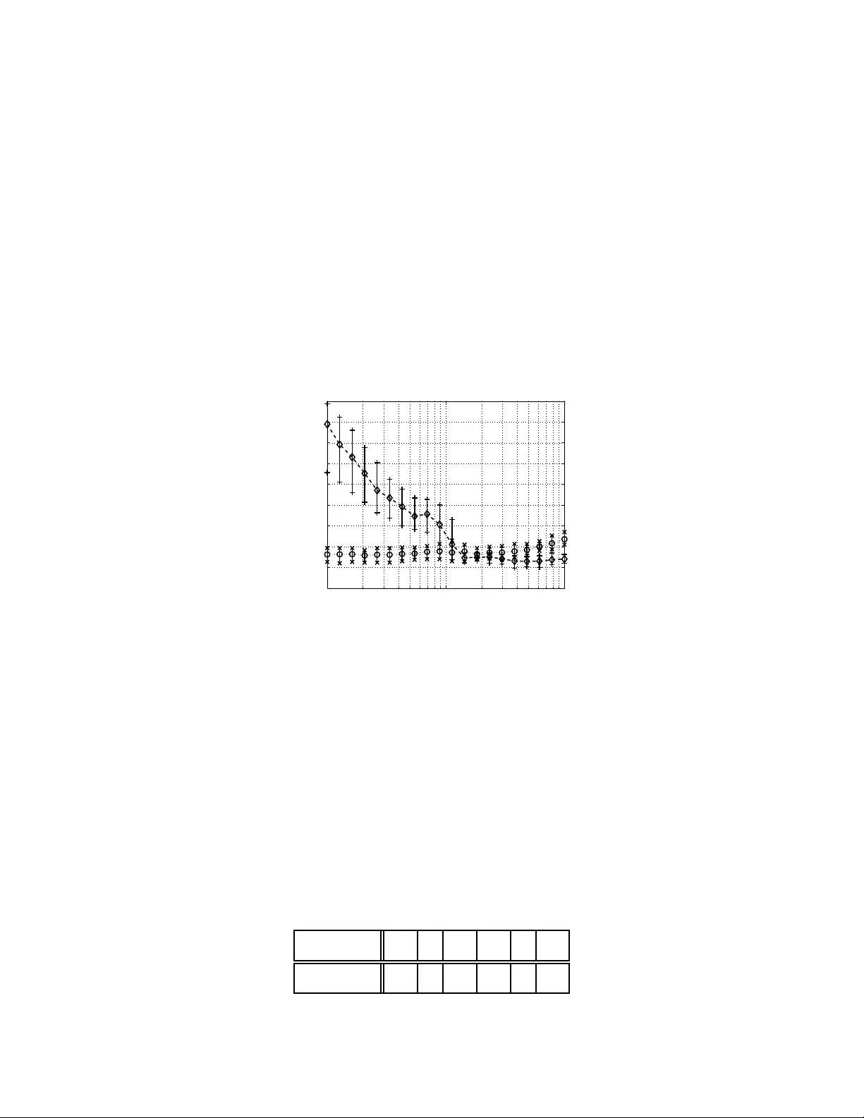
Classification Constrained Dimensionalit y Reduction Ravi v Raich, Member , IEEE, Jose A. Costa, Membe r , IEEE, Ste ven B. Da melin, Senior Member , IEEE, and Alfre d O. Hero I II, F e llow , IEEE Abstract Dimensionality reduction is a topic of recen t interest. In this paper, we present the classification constrained dimensiona lity reductio n (CCDR) algor ithm to accou nt f or lab el information. The a lgorithm can accou nt for multiple classes as well as the sem i-supervised setting. W e pre sent an out-of -sample expressions for both labeled and unlabeled data. For unlabeled data, we introduce a method of embedding a ne w point a s prepro cessing to a classifier . F o r labeled d ata, we introduce a method that improves the embedd ing during th e training p hase using the out-o f-sample extension. W e investigate classification perfor mance using the CCDR algorithm on hy per-spectral satellite imagery data. W e demonstrate the perform ance g ain for both local and g lobal classifiers and demonstrate a 10% improvement of the k -nearest n eighbo rs algorithm p erforman ce. W e present a conn ection between intrinsic dimension estimation and the optima l embedd ing dimension obtained u sing the CCDR algorithm . Index T erms Classification, Computatio nal Complexity , Dimensio nality Reduction, Embedd ing, High Dimen- sional Data, K ernel, K-Nearest Neigh bor, Manifold Learn ing, Pr obability , Out-of-Sam ple Extension . This work was partially funded by the DARP A Defense Sciences Office under Office of Naval Research contract #N00014- 04-C-0437. Distribution S tatement A. Approv ed for public release; distribution is unlimited. S. B. Damelin was supported in part by National Science Foundation grant no. NSF- DMS-055583 9 and NS F-DMS-0439734 and by AFR L. R. Raich is with t he Oregon S tate Univ ersity , Corvallis. A. O Hero III is with the Univ ersity of Michigan, Ann Arbor . J. A. Costa is with the California Institute of T echnology . S. B. Damelin is with the Georgia Southern Univ ersi ty . May 29, 2018 DRAFT 1 Classification Constrained Dimensionalit y Reduction I . I N T R O D U C T I O N In classification theory , th e main goal is to find a mapping from an observa tion space X consisting of a collection o f points in some containi ng Euclidean space R d , d ≥ 1 into a s et consisting of sev eral dif ferent integer v alued hypotheses. In some problems, the observ ations from the set X lie on a d -di mensional manifold M and Whit ney’ s theorem tells us that provided that this manifold is smooth enough, there e xists an embedding of M into R 2 d +1 . This motiv ates the approach t aken by kernel methods in classification theory , such as support vector machines [1] for example. Our interest is in finding an embedding of M into a lower dimens ional Euclidean space. −8 −6 −4 −2 0 2 4 6 8 −8 −6 −4 −2 0 2 4 6 8 P S f r a g r e p l a c e m e n t s e 1 e 2 Fig. 1. PCA of a two-classes classification problem. Dimensionali ty reducti on of high dimensi onal data, was addressed in classical method s such as principal component analysis (PCA) [2] and mu ltidimensi onal scaling (MDS) [3], [4]. In PCA, an eigendecomposition of the d × d empirical cov ariance m atrix i s performed and the data point s are linearly projected along t he 0 < m ≤ d eigen vectors with t he lar gest eigen values. A problem that may occur with PCA for class ification is demon strated in Fig. 1. When the information that is relev ant for classification is present only in the eigen vectors associated with the small eigen values ( e 2 in the figure), remova l of such eig en vectors may result in severe degradation May 29, 2018 DRAFT 2 in classi fication performance. In MDS, t he goal is to find a lower dim ensional embedding of the original data points that preserves the relati ve d istances between all the data points. Th e two later methods suffer greatly when the manifold is no nlinear . For example, PCA will not be able to of fer dim ensionality reductio n for classification of two classes lying each on one of two concentric ci rcles. In [5], a nonl inear extension t o PCA is presented. The algorit hm is based on the “k ernel trick” [6]. Data points are nonlinearly mapped into a feature space, which i n general has a hig her (or e ven in finite) dimension as com pared with the original space and then PCA is applied to the high di mensional data. In the paper of T enenbaum et al [7], Isom ap, a global dim ensionality reduction algorithm was introduced taki ng into account the fact that data points m ay lie o n a lower dimension al manifold. Unlike MDS, geodesic di stances (distances that are measured along th e manifold) are preserved by Isom ap. Isomap ut ilizes the classi cal MDS alg orithm, but instead of usi ng the matrix of Euclidean distances, it uses a m odified version of it. Each point is conn ected on ly to poi nts in its local neighborhood. A dis tance between a point and another poin t outside its local neighborhood is replaced with the s um of distances along t he shortest path in graph. This procedure m odifies the squared dist ances matrix replacing Eucl idian wit h geodesic distances. In [8], Belkin and Niyogi present a related Laplacian eigenmap dimensionalit y reduction algorithm. The algorithm performs a minim ization on the weighted sum of s quared-distances of the lower -dimensi onal data. Each weight m ultiplyin g the squared-distances of two l ow- dimensional data points is in versely related to dis tance bet ween the corresponding two high- dimensional data poi nts. Therefore, sm all distance between two hi gh-dimensional d ata points results in small distance between two l ow-dimensional data points. T o preserve the geodesic distances, th e weight of the distance between two points that do not s hare a local neighborhood is set to zero. W e refer the interested reader to t he references below and t hose cited therein for a list of some of the most commo nly used addi tional algorit hms with in the class o f manifold learnin g algorithms and their different advantages releve nt to our work. Lo cally Linear E mbedding (LLE) [9], Lapl acian Eigenmaps [8], Hess ian Eigenmaps (HLLE) [10], Local Space T angent Analysi s [11], Diffusion M aps [12] and Semidefinite Embedding (SDE) [13]. The algorithm s ment ioned above, consi der the probl em of learning a l ower -dimensional em- May 29, 2018 DRAFT 3 bedding of the data. In classification, such algo rithms can be used to preprocess hi gh-dimensional data before performing the classification. This cou ld potentially allow for a l ower compu tational complexity of the classifier . In some cases, dimensio nality reduction results increase the computa- tional complexity of the classifier . In fact, suppo rt vector machines s uggest the opposing strategy: data points are projected ont o a high er -di mensional space and classified by a low computational complexity classi fier . T o guarantee a low computation al complexity of the classi fier of the low- dimensional data, a class ification constrained dimensi onality reducti on (CCDR) algorithm was introduced in [14]. The CCDR algorith m is an extension of Lapl acian eigenmaps [8] and it incorporates class label information int o the cost function , reducing t he di stance between points with si milar label. Anot her algorit hm that incorporates l abel in formation i s the marginal fisher analysis (MF A) [15], in which a cons traint on the margin between classes is used to enforce class separation. In [14] the CCDR algorithm was only st udied for two classes and i ts performance was illustrated for simulated data. In [16], a multi-class extension to the problem was presented. In this paper , we introdu ce two additional com ponents that m ake the algorithm computationally viabl e. The first is an out-of-sample extension for classification of unlabeled t est poi nts. Similarly to the out-of-sample extension presented in [17], one can utilize the Nys tr ¨ om formula for classification problems in which l abel informatio n is av ailabl e. W e s tudy the algori thm performance as its var ious parameters, (e.g., dimens ion, label im portance, and local neighborhood), are varied. W e study the performance of CCDR as preprocessing prior to im plementation of several classi- fication algorithms such as k -nearest neighbors, linear classification, and neural networks. W e demonstrate a 10% im provement o ver th e k -nearest nei ghbors algo rithm performance benchmark for this dataset. W e add ress the issue of dimens ion estimati on and its effec t on classification performance. The or ganization of this paper i s as follows. Section III presents th e m ultiple-class CCDR algorithm. Section ?? p rovides a s tudy of the alg orithm u sing the Landsat dataset and Section VI s ummaries ou r results. I I . D I M E N S I O N A L I T Y R E D U C T I O N Let X n = { x 1 , x 2 , . . . , x n } be a set of n po ints cons trained to l ie o n an m -dimensi onal submanifold M ⊆ R d . In dimensi onality reduction, ou r goal is to obtai n a lower -dimensional May 29, 2018 DRAFT 4 embedding Y n = { y 1 , y 2 , . . . , y n } (where y i ∈ R m with m < d ) that preserves local geometry information such that processing of the lower dimensio nal em bedding Y n yields comparable performance to processing of the original data points X n . Al ternativ ely , we would like learn the mappi ng f : M ⊆ R d → R m that maps e very data po int x i to y i = f ( x i ) such that some geometric properties of th e high-dimension al data are preserved in the lower dim ensional embedding. The first question that comes to mi nd is how to select f , or m ore s pecifically how to restrict th e functi on f so that we can still achieve our goal. A. Linear dimensi onality r edu ction 1) PCA: Wh en principal component analysis (PCA) is used for dimensionality reduction, one considers a lin ear embeddin g of t he form y i = f ( x i ) = Ax i , where A is m × d . T his embedding captures the notion of proxim ity in the sense that clos e points in the high dim ensional space m ap to close p oints i n the lower dimension al embedding, i.e., k y i − y j k = k A ( x i − x j ) k ≤ k A kk x i − x j k . Let ¯ x = 1 n n X i =1 x i and C x = 1 n n X i =1 ( x i − ¯ x )( x i − ¯ x ) T . Similarly , let ¯ y = 1 n n X i =1 y i and C y = 1 n n X i =1 ( y i − ¯ y )( y i − ¯ y ) T . Since y i = Ax i , we have ¯ y = A ¯ x and C y = A C x A T . In PCA, t he goal is t o find th e projection matrix A that preserves mos t of the ener gy in the original data by s olving max A tr {C y ( A ) } s.t. AA T = I , which is equivalent to max A tr { A C x A T } s.t. AA T = I . (1) May 29, 2018 DRAFT 5 The solutio n to (1), is giv en by A = [ u 1 , u 2 , . . . , u m ] T , w here u i is the eigen vector of C x corresponding to its i th largest eigen va lue. When the data lies on an m -dimensional hyperplane, the matrix C x has only m positive eigen values and the rest are zero. Furthermore, e very x i belongs to ¯ x + span { u 1 , u 2 , . . . , u m } ⊆ R d . In this case, the mappin g PCA finds f ( x ) = Ax is one-to-one and s atisfies k f ( x i ) − f ( x j ) k = k A ( x i − x j ) k = k x i − x j k . Therefore, the lower embedding preserves all the geometry i nformation in the origin al dataset X . W e would li ke t o point out th at PCA can be written as max {Y } n X i =1 k y i − y j k 2 s.t. y i = A x i and AA T = I , 2) MDS: Mul tidimensi onal Scaling (M DS) di f fers from PCA in the way th e input is provided to i t. Whi le in PCA, t he original data X is provided, the classical MDS requires only the set of all Euclid ean pairwise distances {k x i − x j k 2 } n − 1 i =1 ,j >i . As MDS uses onl y pairwise distances, the solut ion it finds is giv en up to t ranslation and u nitary transformati on. Let x ′ i = x i − c , the Euclidean dis tance k x ′ i − x ′ j k is the same as k x i − x j k . Let U be an arbitrary un itary matrix U satisfying U T U = I and define x ′ i = U x . The distance k x ′ i − x ′ j k i s equal to k U ( x i − x j ) k , which by th e in variance of t he Euclidean n orm to a uni tary transform ation equals to k x i − x j k . Denote the pairwise squared-distance matrix by [ D 2 ] ij = k x i − x j k 2 . By the definition of Euclidean dis tance, t he matrix D 2 satisfies D 2 = 1 φ T + φ 1 T − 2 X T X , (2) where X = [ x 1 , x 2 , . . . , x n ] and φ = [ k x 1 k 2 , k x 2 k 2 , . . . , k x n k 2 ] T . T o verify (2), one can examine the ij -th term of D 2 and compare with k x i − x j k 2 . Denote the n × n matrix H = I − 11 T /n . Mul tiplying both sides of D 2 with H in addition t o a factor of − 1 2 , yields − 1 2 H D 2 H = ( X H ) T ( X H ) , which is key t o MDS, i.e., Cholesky decomposi tion of − 1 2 H D 2 H yields X to within a trans- lation and a u nitary transform ation. Consider the eigendecompo sition − 1 2 H D 2 H = U Λ U T . Therefore, a rank d X can be obtained as X = Λ 1 2 d U T d , where Λ d = dia g { [ λ 1 , λ 2 , . . . , λ d ] } 1 2 and U d = [ u 1 , u 2 , . . . , u d ] . No te that X H is a translated version of X , in which ev ery column x i is transl ated to x i − ¯ x . T o use MDS for di mensionality reduction, we can consider a tw o step process. First a square- distance matrix D 2 is obtained from the high-di mensional data X . Then, MDS is applied to D 2 May 29, 2018 DRAFT 6 to o btain a low-dimensional ( m < d ) embedding by X m = Λ 1 2 m U T m = X U m U T m . In the absence of no ise, t his procedure provides an affine transformation to the hi gh-dimensional data and thus can be regarded as a linear method. B. Nonlinear di mensionality r educti on Linear m aps are limit ed as t hey cannot preserve the g eometry of nonl inear manifolds. 1) Ke rnel PCA: Ke rnel PCA is one of the first m ethods i n dimensionali ty reduction of data on nonli near manifolds. The met hod combin es the dimensi onality reduction capabilities of PCA on linear manifolds with a nonlinear embeddi ng of data po ints in a higher (or e ven infinite) dimensional space usin g “kernel trick” [6]. In PCA, one finds the eigen vectors satisfyi ng: C x v k = λ k v k . Since v k can be writ ten as a linear combinatio n of the x i ’ s: v k = P i α k i ( x i − ¯ x ) , one can replace v k in the eigendecomposition , simp lify , and obtain: X ( K α k − λ k α k ) = 0 , where K ij = ( x i − ¯ x ) T ( x j − ¯ x ) . Consid er the mappi ng φ : M → H from the manifold to a Hil bert space. The “kernel trick” suggests replacing x i with φ ( x i ) and therefore rewriting the kernel as K ij = φ ( x i ) T φ ( x j ) . Further generalizatio n can be made by s etting K ij = K ( x i , x j ) where K ( · , · ) is positive sem idefinite. The resulting vectors are of the form v k = P i α k i φ ( x i ) and thus i mplementing a nonlinear embeddi ng into a no nlinear manifol d. 2) ISOMAP: In [7], T enenbaum et al find a non linear emb edding that rather than preserving the Euclidean dist ance between points on a manifold, p reserves the geodesic dist ance between points on th e manifold. Sim ilar to MD S where a lower dimens ional embedding is found to preserve the Eu clidean dist ances of hig h dimens ional data, ISOMAP finds a l ower dim ensional embedding that preserves the geodesi c di stances between high-dimensi onal data points. 3) Laplacia n Eigenmaps: Belkin and Niyogi’ s Laplacian eigenmaps dim ensionality reduction algorithm [8] takes a different approach. They consider a nonlinear mappin g f that minimi ze the Laplacian arg min k f k L 2 ( M ) =1 Z M k∇ f k 2 . (3) Since the manifold is not a va ilable b ut only data point on it are, the lo wer dimensional embedding is found b y mini mizing the graph Laplacian given by n X i =1 w ij k y i − y j k 2 , (4) May 29, 2018 DRAFT 7 where w ij is the ij th element of the adjacency matrix which is constructed as follows: For k ∈ N , a k -nearest neighbors graph is constructed wit h the p oints in X n as t he graph vertices. Each point x i is connected t o i ts k -nearest neighbo ring point s. Note t hat i t suffi ces that eith er x i is among x j ’ s k -nearest neighbors or x j is among x i ’ s k -nearest neighbo rs for x i and x j to be conn ected. For a fixed scale parameter ǫ > 0 , the weight associat ed wit h the two points x i and x j satisfies w ij =    exp {−k x i − x j k 2 /ǫ } if x i and x j are connected 0 otherwise. I I I . C L A S S I FI C A T I O N C O N S T R A I N E D D I M E N S I O N A L I T Y R E D U C T I O N A. Statistical framework T o put the probl em in a classification con text, we consider the following model. Let X n = { x 1 , x 2 , . . . , x n } b e a set of n point s sampled from an m -dim ensional submanifold M ⊆ R d . Each point x i ∈ M is associate with a class l abel c i ∈ A = { 0 , 1 , 2 , . . . , L } , where c i = 0 corresponds to th e case of unlabeled data. W e assume that pairs ( x i , c i ) ∈ M × A are i.i.d. drawn from a j oint distribution P ( x , c ) = p x ( x | c ) P c ( c ) = P c ( c | x ) p x ( x ) , (5) where p x ( x ) > 0 and p x ( x | c ) > 0 (for x ∈ M ) are the marginal and the conditio nal probability density functions, resp ecti vely , sati sfying R M p x ( x ) d x = 1 , R M p x ( x | c ) d x = 1 and P c ( c ) > 0 and P c ( c | x ) > 0 are t he a priori and a post eriori probabili ty mass functions of the class label, respectiv ely , satisfyin g P c P c ( c ) = 1 and P c P c ( c | x ) = 1 . While we cons ider u nlabeled poin ts of t he form ( x i , 0) simi lar labeled point s, we still make the following d istinction. Consider the following m echanism for generating an u nlabeled poin t. First, a class label c ∈ { 1 , 2 , . . . , L } is generated from the labeled a p riori probabil ity m ass functio n P ′ c ( c ) = P ( c | c is labeled ) = P c ( c ) / P L c ′ =1 P c ( c ′ ) . T hen x i is generated according to p x ( x | c ) . T o t reat c as an unobserved label, we marginalize P ( x , c | c is labeled ) = p x ( x | c ) P ′ c ( c ) over c : p x ( x | c = 0) = L X q =1 p x ( x | c = q ) P ′ c ( q ) = P L q =1 p x ( x | c = q ) P c ( q ) P L c ′ =1 P c ( c ′ ) . (6) This suggests that the conditional PDF of unlabeled points f x ( x | c = 0) i s uniquely determined by the class pri ors and the conditionals for labeled point. W e would like to point out that this is one May 29, 2018 DRAFT 8 of few treatments that can be o f fered for unlabeled po int. For example, in anomaly detection , one m ay want t o ass ociate the unlabeled point wit h contaminated data po ints, which can be represented as a densit y mix ture of p x ( x | c = 0) and γ ( x ) (e.g., γ ( x ) i s uniform in X ). In classification con straint dimensionalit y reducti on, our g oal is to obtain a lower -dimens ional embedding Y n = { y 1 , y 2 , . . . , y n } (where y i ∈ R m with m < d ) that preserves local geometry and that encourages clustering of points of the same class label . Alternative ly , we would like to find a m apping f ( x , c ) : M × A → R m for which y i = f ( x i , c i ) that is s mooth and that clusters poi nts of the same label. W e introduce the class label indicator for data point x i as c k i = I ( c i = k ) , for k = 1 , 2 , . . . , L and i = 1 , 2 , . . . , n . N ote that when point x i is unlabeled c k i = 0 for all k . Using the class indicator , we can write the n umber of poi nt i n class k as n k = P n i =1 c k i . If all points are labeled, then n = P L k =1 n k . B. Linear dimensi onality r edu ction for classi fication 1) LDA: Restricting the discussion to li near maps, one can extend PCA to take into account label informati on using t he m ulti-class extension to Fisher’ s linear di scriminant analysis (LD A). Instead of maximizing t he d ata covariance m atrix, LD A maximizes the ratio of the between- class-cov ariance to within-class-covariance. In oth er words, we obtain a linear transformation y i = f ( x i , c i ) = Ax i with m atrix A that is the so lution to th e following maximization : max A tr { A C B A T } s.t. A C W A T = I , (7) where C B = 1 n L X k =1 n k ( ¯ x ( k ) − ¯ x )( ¯ x ( k ) − ¯ x ) T is t he between-class-covariance matrix, ¯ x ( k ) = P i c k i x i /n k is t he k th class center , ¯ x = P i x i /n is the center point of the dataset, C W = 1 n L X k =1 n k C ( k ) W , is the wit hin-class-cov ariance, and C ( k ) W = P n i =1 c k i ( x i − ¯ x ( k ) )( x i − ¯ x ( k ) ) T n k May 29, 2018 DRAFT 9 is wi thin-class- k cov ariance matrix. In Fig. 1, LD A selects an emb edding t hat proj ects the data onto e 2 since the maximum distance betw een classes is achie ved along with a m inimum class va riance when projecting the data ont o e 2 . W e are interested in exploring a strategy that maximizes class separation in the lower dimensio nal embedding. 2) Mar ginal F isher Anal ysis: Recent work [15], presents the mar g inal Fis her analysis (MF A), which is a method t hat m inimizes the ratio between intraclass com pactness and interclass separability . In its basic formulation MF A is a linear embedding , i n which y i = Ax i . An other aspect of the m ethod is that i t considers two classes. The kernel trick i s used to provide a nonlinear extension to MF A. T o construct the cost function , two quantities are of i nterest: intraclass compactness and in terclass separability . The intraclass compactness can be written as X i,j w ij k y i − y j k 2 , (8) where w ij is give n by w ij = ( X k c k i c k j ) I ( x i ∈ N + k 1 ( x j ) or x j ∈ N + k 1 ( x i )) (9) and N + k ( x ) denote the k -nn neigh borhood of x within the same class as x . Note t hat the term P k c k i c k j is one if x i and x j hav e the same label and zero otherwise. Similarly , the int erclass separability can be writt en as X i,j w ij k y i − y j k 2 , (10) where w ij is give n by w ij = (1 − X k c k i c k j ) I ( x i ∈ N − k 2 ( x j ) or x j ∈ N − k 2 ( x i )) (11) and N − k ( x ) denote t he k -nn neighb orhood of x ou tside th e class of x . I V . D I M E N S I O N A L I T Y R E D U C T I O N F O R C L A S S I FI C A T I O N O N N O N L I N E A R M A N I F O L D S Here, we revie w the CCDR algorithm [14] and it s extension to multi -class classification. T o cluster lower dimensional embedded points o f the same label we associate each class with a class center namely z k ∈ R m . W e construct the fol lowing cos t function: J ( Z L , Y n ) = X k i c k i k z k − y i k 2 + β 2 X ij w ij k y i − y j k 2 , (12) May 29, 2018 DRAFT 10 where Z L = { z 1 , . . . , z L } and β ≥ 0 is a regularization parameter . W e cons ider two terms on the RHS of (12). The first term corresponds t o the concentration of p oints of the same label around their respective class center . T he second term is as i n (4) or as in Laplacian Eigenmaps [8] and controls the sm oothness of the embedding ove r the manifold. Lar ge values of β produ ce an embedding that ignores class labels and small v alues of β produce an embedding that ignores the manifol d structure. Training data points wi ll tend to collapse into the class centers, allowing many classifiers to produce perfect classification on the training data without being able to control the generalization error (i.e., class ification error o f the unlabeled data). Our goal is to find Z L and Y n that mi nimize t he cost function in (12). Let C be the L × n class membership matrix with c k i as its k i -th e lement, Z = [ z 1 , . . . , z L , y 1 , . . . , y n ] , and 0 b e th e L × L all zeroes matrix and G =   0 C C T β W   . Minimizati on over Z of the cost function in (12) can be expressed as min Z D 1 = 0 Z D Z T = I tr  Z LZ T  , (13) where D = diag { G 1 } and L = D − G . T o prev ent the lower -di mensional points and the class centers from collapsin g into a single point at the origi n, the regularization Z D Z T = I is int roduced. The second constraint Z D 1 = 0 is con structed to prev ent a degenerate solution , e.g., z 1 = . . . = z L = y 1 = . . . = y n . T his solu tion m ay occur since 1 is in the null -space of the Laplacian L operator , i.e., L 1 = 0 . The solu tion to (13) can be expressed in term of the following generalized eigendecomp osition L ( n ) u ( n ) k = λ ( n ) k D ( n ) u ( n ) k , (14) where λ ( n ) k is the k th eigen value and u ( n ) k is its corresponding eigen vector . Note that we include ( n ) to emph asize the dependence on t he n data points. Without l oss of generality we assume λ 1 ≤ λ 2 ≤ . . . ≤ λ n + L . Specifically , matrix Z is giv en by [ u 2 , u 3 , . . . , u m +1 ] T , where the first L columns correspond to the coordinates of the class centers, i. e., z k = Z e k , and the following n columns determine the embeddi ng of the n data p oints, i.e., y t = Z e L + t . W e u se e i to denote the canonical vector such th at [ e i ] s = 1 for element s = i and zero otherwise. May 29, 2018 DRAFT 11 A. Classification and computa tional complexity In classi fication, the goal is to find a classifier a x ( x ) : M → A based on the traini ng data that mi nimizes the generalization error: ˆ a = a rg min a ∈F E [ I ( a ( x ) 6 = a )] , (15) where the expectation is taken w .r .t. t he pair ( x , a ) . Since only sam ples from the joint d istribution of x and a are av ailable, we replace the expectation with a sample av erage w . r . t. th e training data 1 n P n i =1 I ( a ( x i ) 6 = a i ) . During t he minimizati on, we s earch over a set of classifiers a x ( x ) : M ⊆ R d → A , which i s defined over a dom ain in R d . In our framework, we s uggest replacing a classifier a x ( x ) : M ⊆ R d → A w ith dimensio nality reduction via CCDR f ( x ) : M ⊆ R d → R m followed by a classifier o n the lowe r -dimensional space a y ( y ) : R m → A , i.e., a x = a y ◦ f . The first advantage is that the search space for the m inimization in (15) defined over a d -dim ensional space can be reduced to an m -dimensional space. This resul ts in si gnificant savings i n comput ational complexity if the complexity associated wi th the process of obt aining f can be made low . In general, the classifier set F h as to be rich enou gh to attain a lower generalization error . The ot her advantage of our m ethod lies in the fact that CCDR is designed to cluster poi nts of the same label thus allowing for a l inear classifier or o ther l ow complexity classifiers. T herefore, furth er reduction i n th e size of class F can be achieved in addit ion to the reduction due to a lower -dimensional domain. T o classify a new data point, one has t o apply CCDR to a new data point. If it is do ne brute force, the point i s added to the set of training points wit h no label a new matrix W ′ is formed and an eigendecomposit ion is carried out . When performing CCDR, each of the n ( n − 1) / 2 terms of the form {k x i − x j k 2 } requires one summatio n and d m ultiplicati ons leading to computational com plexity of the order O ( dn 2 ) . Construction of a K -nearest neighbors graph requires O ( kn ) comparisons p er point and therefore a total of O ( k n 2 ) . The total number of operation s in volv ed in constructing the graph is t herefore O (( k + d ) n 2 ) . Next, an ei gendecomposition is applied to W ′ , which is an ( L + n ) × ( L + n ) matrix. The associated com putation complexity is O ( n 3 ) . Therefore, the overall comp utational complexity of CCDR is O ( n 3 ) . Thi s holds for both trainin g and classification as explained earlier . W e are i nterested in reducing com putational complexity in traini ng the classifier and in classification. For that pu rpose, we consider an out-of-sampl e extension of CCDR. May 29, 2018 DRAFT 12 V . O U T - O F - S A M P L E E X T E N S I O N W e start by rearranging the generalized eigendecomp osition of the Laplacian in (14 ) as G ( n ) u ( n ) l = (1 − λ ( n ) l ) D ( n ) u ( n ) l , (16) and recall th at u ( n ) l = [ z 1 ( l ) , z 1 ( l ) , . . . , z 1 ( l ) , y 1 ( l ) , y 2 ( l ) , . . . , y n ( l ) ] T . Since we consid er an m - dimensional embeddi ng, we are o nly i nterested in eigen vectors u 2 , . . . , u m +1 . The L + i equatio n (ro w) for i = 1 , 2 , . . . , n in the eigendecomposi tion in (16) can b e writt en as y ( n ) i ( l ) = 1 1 − λ ( n ) l P k c k i z ( n ) k ( l ) + β P j K ( x i , x j ) y ( n ) j ( l ) P k c k i + β P j K ( x i , x j ) . (17) Similarly , the k th equation (row) of (16) for k = 1 , 2 , . . . , L is given b y z ( n ) k ( l ) = P i c k i y ( n ) i ( l ) (1 − λ ( n ) l ) n k . (18) Our interest is i n finding a mappi ng f ( x , c ) that i n additi on to mapping ev ery x i to y i , can perform an out-of-sampl e extension, i.e., is well-defined out side the set X . W e consi der the following out-of-sample extension expression f ( n ) l ( x , c ) = 1 1 − λ ( n ) l I ( c 6 = 0) z ( n ) c ( l ) + β P j K ( x , x j ) y ( n ) j ( l ) I ( c 6 = 0) + β P j K ( x , x j ) , (19) where z ( n ) is the sam e as in (18). This form ula can be explain as foll ows. First, the l owe r dimensional emb edding y ( n ) 1 , . . . , y ( n ) n and the class centers z ( n ) 1 , . . . , z ( n ) L are obtain ed through an the eigendecompositi on in (16). Then, the embedding outside the sam ple set X is calculated via (19). By comparison of f ( n ) l ( x i , c i ) e va luated through (19) with (17), we ha ve f ( n ) l ( x i , c i ) = y ( n ) i ( l ) . This suggests t hat t he ou t-of-sample extension coincides wit h t he so lution, we already hav e for the mapping at th e the data points X . Moreover , using this result one can replace all y ( n ) i with f ( n ) l ( x i , c i ) i n (19) and obtain the following generalization of t he eigendecompositio n in (16): f ( n ) l ( x , c ) = 1 1 − λ ( n ) l I ( c 6 = 0) z ( n ) c ( l ) + β P j K ( x , x j ) f ( n ) l ( x j , c j ) I ( c 6 = 0) + β P j K ( x , x j ) , (20) and z ( n ) k ( l ) = P i c k i f ( n ) l ( x i , c i ) (1 − λ ( n ) l ) n k . (21) May 29, 2018 DRAFT 13 In [18], it is propose that if the out-of-sam ple solutio n to the eigendecompo sition problem associated with kernel PCA con ver ge, it i s given by the soluti on to the asym ptotic equivalent of t he eigendecom position. Usi ng s imilar m achinery , we can provide a simi lar result suggesting that if f ( n ) l ( x , c ) → f ( ∞ ) l ( x , c ) as n → ∞ , then the asym ptotic equiv alents to (20) and (21) should provide t he so lution to the limit of f ( n ) l ( x , c ) . The asymptotic analo gues to (17) and (18) are described in th e following. The mapping for l abeled data f l ( x , c ) : M × A → R for c = 0 , 1 , 2 , . . . , L equiv alent to equatio n (17) is f l ( x , c ) = 1 1 − λ l I ( c 6 = 0) z c ( l ) + β ′ P L c ′ =0 R M K ( x , x ′ ) f l ( x ′ , c ′ ) P ( x ′ , c ′ ) d x ′ I ( c 6 = 0) + β ′ R M K ( x , x ′ ) p ( x ′ ) d x ′ (22) where z c ( l ) for c = 1 , 2 , . . . , L is equiv alent to (18) z c ( l ) = R M f l ( x , c ) p ( x | c ) d x 1 − λ l , (23) and β ′ = β n . Since we are in terested in an m -dimensio nal embedding, we consider o nly l = 1 , 2 , . . . , m , i. e., the eigen vectors th at correspond t o the m smallest eigen values. T o guarantee that the relev ant eig en vectors are unique (up to a multipl icativ e constant), we require λ 1 < λ 2 < · · · < λ m +1 ≤ λ m +2 ≤ . . . λ n . The o ut-of-sample extension giv en by (19), can be useful in a coupl e of s cenario. The first, is in classification of new unlabeled samples. W e assume th at { y j } n j =1 , { z k } L k =1 , and { λ l } m l =1 are already obtained based on labeled (or partially l abeled) traini ng data and we would l ike to embed a ne w unlabeled data po int. W e consi der using (19) wi th c = 0 , i.e., we can use f ( x , 0) to map a new s ample x to R m . The obvious immediate advantage is the savings in compu tational complexity as we av oid performing addition eigendecomp osition that includes the new point. The s econd scenario in volv es the out-of-sample extension for labeled data. The goal here is not to classify the data si nce the label is already a vailable. Inst ead, we are interested in the training ph ase in the case of large n for which the eigendecomposition is infeasible. In t his case, a large amount of labeled training data is ava ilable but due to t he heavy computation al complexity associated with the eigendecompos ition in (14) (or by (16)), the data cannot be processed. In this case, we are interested in developing a resampling method, which i ntegrates f ( n ) l ( x , c ) obtained for different subsamples of the complet e data set. May 29, 2018 DRAFT 14 A. Classification Algori thms W e consid er three widespread algori thms: k -neare st neighbors, linear classification , and neural networks. A standard implement ation of k -nearest n eighbors was u sed, see [1, p. 415]. The linear classifier we im plemented is give n by ˆ c ( y ) = arg max c ∈{A 1 ,... A L } y T α ( c ) + α ( c ) 0  α ( A k ) , α ( A k ) 0  = arg min [ α ,α 0 ] n X i =1 ( y T i α + α 0 − c k i ) 2 , for k = 1 , . . . , L . The neural network we im plemented is a three-layer n eural network with d elements in the input layer , 2 d elements in t he hidden layer , and 6 elements i n the outp ut layer (one for each class). Here d was selected usin g the comm on PCA procedure, as the smallest dimension t hat explains 99 . 9% of t he energy o f the d ata. A gradient metho d was used to train the network coefficients with 2000 i terations. The neural net is significantly more comp utationally burdensome than either li near or k -n earest neighb ors classifications algorithms. B. Data Descrip tion In thi s secti on, we examine the performance of the classification algori thms on the benchmark label classification problem provided by the Landsat MSS satell ite i magery d atabase [19]. Each sample point consists of th e intensit y values of one pixel and its 8 n eighboring pixels in 4 diffe rent spectral bands. T he training data cons ists of 4435 36-di mensional points of whi ch, 1072 are labeled as 1) red soil , 479 as 2 ) cotton crop, 961 as 3) grey soil, 415 as 4) damp grey soi l, 470 are labeled as 5) so il wi th vegetation stubb le, and 1038 are labeled as 6) very damp grey soil. The test data consi sts of 2000 36-dim ensional po ints of which, 461 are labeled as 1) red soil, 2 24 as 2) cotton crop, 397 as 3 ) grey soil, 211 as 4) dam p grey soil, 237 are labeled as 5) soil with vegetation stubbl e, and 470 are labeled as 6) very damp grey soil . In the following, each classifier i s trained on th e traini ng data and its classification is ev aluated based o n t he enti re sampl e test data. In T able I, we present “best case” performance of neural networks, l inear classifier , and k -nearest n eighbors in three cases: no dim ensionality reducti on, dimensionali ty reduction v ia PCA, and dim ensionality reduction via CCDR. The table presents the minimum probabilit y o f error achie ved by varying the tuni ng parameters of t he class ifiers. May 29, 2018 DRAFT 15 The benefit of usin g CCDR is obvious and we are prompted to further ev al uate the performance gains attai ned using CCDR. Neural Net. Lin. k -nearest neigh. No dim. reduc. 83 % 22.7 % 9.65 % PCA 9.75 % 23 % 9.35 % CCDR 8.95 % 8.95 % 8.1 % T ABLE I C L A S S I FI C A T I O N E R RO R P R O BA B I L I T Y C. R e gularizat ion P arameter β As mentioned earlier , the CCDR regularization parameter β con trols the contribution of the label inform ation versus th e contribution of the geometry described by the sam ple. W e apply CCDR to the 36-dimensi onal data to create a 14 -dimensional embeddin g by varying β over a range of values. For justi fication of our choice of d = 14 dim ensions see Section V -D. In the process o f computing the weight s w ij for the alg orithm, we us e k -nearest neighbors with k = 4 to determi ne the local neighborhood. Fig. 2 shows the class ification error p robability (dashed lines) for the linear classifier vs. β after preprocessing the data us ing CCDR with k = 4 and dimension 14. W e observe that for a large range of β the av erage cl assification error probability is g reater th an 0 . 09 but smaller than 0 . 0 95 . T his performance competes with the performance of k -nearest neighbors appli ed to the high-dimensi onal d ata, whi ch is presented in [1] as the leading classifier for this benchmark problem . Anot her observation i s that for small values of β (i.e., β < 0 . 1 ) the probabi lity of error is constant . For such small value of β , classes in the l ower -dimensional embedding are well-separated and are well-concentrated around the class centers. Therefore, the li near classifier yields perfect classi fication on the traini ng set and fairly low const ant probabili ty of error on the test data is attained for low value of β . When β is increased, we n otice an increase in the classification error probability . This is due to the fact that the traini ng data become non separable by any l inear classi fier as β increases. W e perform a simi lar st udy of classification performance for k -nearest neigh bors. In Fig. 2, classification probability error is plotted (dotted lines) vs . β . Here, we observed that an a verage May 29, 2018 DRAFT 16 error probabil ity of 0 . 086 can be achie ved for β ≈ 0 . 5 . Therefore, k -nearest neighbors preceded by CCDR o utperforms th e straightforward k -neare st neighb ors algorithm. W e als o observe that when β is decreased the probabi lity of error is increased. Thi s can be explained as due to the ability of k -neare st neighbors to utilize local inform ation, i.e., local geometry . This information is dis carded when β is decreased. W e con clude t hat CCDR can generate lower -dimensional dat a that i s us eful for global classi - fiers, such as the linear classifier , by using a small value of β , and also for local classifiers, such as k -nearest neighbors, by using a larger value β and thu s preserving local geometry informat ion. 10 −2 10 −1 10 0 0.06 0.08 0.1 0.12 0.14 0.16 0.18 0.2 0.22 0.24 P S f r a g r e p l a c e m e n t s β P(error) Fig. 2. Probability of incorrect classifi cation vs. β for a linear classifier (dotted line ◦ ) and for the k -nearest neighbo rs algorithm (dashed line ⋄ ) preprocessed by CCDR. 80% confidence intervals are presented as × for the l inear classifier and as + for t he k - nearest neighbors algorithm. D. Dimension P arameter While the data poi nts in X n may lie on a manifold o f a parti cular dim ension, t he actual di- mension required for classification may be sm aller . Here, we e xamine classification performance as a function of the CCDR dimensio n. Usi ng the entropic graph dimension estimation algorithm in [20], we obtain the following estimated di mension for each class: class 1 2 3 4 5 6 dimension 13 7 13 10 6 13 May 29, 2018 DRAFT 17 2 4 6 8 10 12 14 0.08 0.1 0.12 0.14 0.16 0.18 0.2 P S f r a g r e p l a c e m e n t s dim. P(error) Fig. 3. Probability of incorrect classification vs. CCDR’s dimension for a linear classifier (dotted line ◦ ) and for the k - nearest neighbors algorithm ( dashed line ⋄ ) preprocessed by CCDR. 80% confidence interv als are presented as × for the linear classifier and as + for the k -nearest neighbors algorithm. Therefore, if an o ptimal nonli near embedding of the data could be found , we suspect t hat a dimension greater than 13 may not yield signi ficant improvement in classification performance. Since CCDR does not necessarily yield an optimal embedding, we choose CCDR embeddi ng dimension as d = 14 in Section V -C. In Fig. 3, we plot th e classification error probabil ity (dott ed line) vs. CCDR dim ension and its confidence int erv al for a linear classifier . W e observed d ecrease in error p robability as the dimension increases. When the CCDR dimensi on is greater t han 5 , the error probability seems fairly con stant. Thi s is an indication that CCDR di mension o f 5 is suf ficient for classi fication if one uses the li near classifier with β = 0 . 5 , i .e., linear classifier cannot exploit geometry . W e also pl ot the classification error probability (dashed line) vs. CCDR dim ension and i ts confidence interval for k -nearest n eighbors class ifier . Generally , we observe decrease in error probability as the dimension increases. When the CCDR d imension is greater than 5 , the error probability seems fairly constant . When CCDR dim ension i s three, classifier error i s below 0 . 1 . On the other hand, minimum p ossibilit y of error ob tained at CCDR d imension 12-14. This is rem arkable agreement with the dimens ion estimat e of 13 obtain ed using the entropic graph algorithm of [20]. May 29, 2018 DRAFT 18 1 2 3 4 5 6 7 8 0.08 0.1 0.12 0.14 0.16 0.18 0.2 P S f r a g r e p l a c e m e n t s K-CCDR P(error) Fig. 4. Probability of incorrect classifi cation vs. CCDR’s k -nearest neighbors para meter for a li near classifier (dotted line ◦ ) and for the k - nearest neighbors algorithm (dashed li ne ⋄ ) preprocessed by CCDR. 80% confidence intervals are presented as × for the li near classifier and as + for the k -nearest neighbors algorithm. E. CCDR’ s k -Near est Neighbors P arameter The l ast parameter we examine is t he CCDR’ s k -nearest neighbors parameter . In general, as k increases non-local distances are included i n t he lower -dimensional embedd ing. Hence, very lar ge k prev ents the flexibility necessary for d imensionalit y reducti on on (globally) non-linear (but locally lin ear) manifold s. In Fig. 4, the classi fication p robability of error for the linear classifier (dot ted l ine) is plotted vs. the CCDR’ s k -nearest neig hbors parameter . A mi nimum is obtain ed at k = 3 with probabil ity of error of 0 . 09 2 . The classification probability of error for k -nearest neighbors (dashed l ine) is plotted vs . the CCDR’ s k -nearest neighbors p arameter . A m inimum is obtain ed at k = 4 with probability of error of 0 . 086 . V I . C O N C L U S I O N In this paper , we presented the CCDR algorithm for multipl e classes. W e examined the per- formance of v arious classification alg orithms applied after CCDR for the Landsat MSS im agery dataset. W e sh owe d that for a linear classifier , decreasing β yields improve d performance and for a k -nearest n eighbors classifier , increasing β yields im proved performance. W e demonst rated that both classifiers have improv ed performance on the m uch smal ler dimension of CCDR em bedding space than when applied to the original high -dimensional data. W e also explored the ef fect of k May 29, 2018 DRAFT 19 in the k -nearest neighbors construction of CCDR weight matrix on classification performance. CCDR all ows reduced comp lexity classification such as the linear classi fier to perform better than more complex classifiers applied to the original data. W e are currently pursuing an out-of- sample extension to the algorit hm that does not require rerunning CCDR on test and training data t o classify new test point. R E F E R E N C E S [1] T . Hastie, R. Tibshirani, and J. Friedman, T he E lements of Statistical Learning D ata Mining, Infer ence, and Pr ediction , ser . Springer Series in S tatistics. Ne w Y ork: Springer V erlag, 2000. [2] A. K. Jain and R. C. Dubes, Algorithms for clustering data . New Jersey: P rentice Hall, 1998. [3] W . S. T orgerson, “Multidimensional scaling: I. theory and method, ” Psychometrika , vol. 17, pp. 401–419, 1952. [4] T . F . Cox and M. A. A. Cox, Multidimensional Scaling , 2n d ed., ser . Monograp hs on Statist ics and Applied Probability . London: Chapman & Hal l/CRC, 2000, vol. 88. [5] B. Sch ¨ olkop f, A. J. Smola, and K. -R. M ¨ uller , “Nonlinear component analysis as a kernel eigen value problem. ” Neura l Computation , vol. 10, no. 5, pp. 1299–1319, 1998. [6] A. Aizerman, E. M. Bra verman, and L. I. Rozoner , “Theoretical foun dations of the potential function method in pattern recognition learning, ” Automation and Remote Contr ol , vol. 25, pp . 821–837, 19 64. [7] J. B. T enenbaum, V . D. Si lv a, and J. C. Langford, “ A global geometric frame work for nonlinear dimensionality reduction. ” Science , vol. 290, no. 5500, pp. 2319–232 3, 2000. [8] M. Belkin and P . Niyogi, “Laplacian eigenm aps for dimensionality reduction and data representation, ” Neural Computation , vol. 15, no. 6, pp. 1373–1396, June 2003. [9] S. T . Ro weis and L. K. Saul, “Nonlinear dimensionality reduction by locally linear embedding, ” Science , vol. 290 , no. 5500, pp. 2323–2326, December 2000. [10] D. L. Donoho and C. Gri mes, “Hessian eigenmaps: Locally linear embedding techniques for high-dimensional data, ” Pr oceedings of the National Academy of Sciences of the United States of America , vol. 100, no. 10, pp. 5591–5596 , May 2003. [11] Z . Zhang and H. Zha, “Pri ncipal manifolds and nonlinear dimensionality reduction via tangent space alignment, ” SIAM J. Sci. Comput. , v ol. 26, no. 1, pp. 313–338, 2005. [12] R. Coifman and S . Lafon, “Diffusion maps, ” Applied and Computational Harmon ic Analysis: Special issue on Diffusion Maps and W avelets , vol. 21, pp. 5–30, July 2006. [13] K. Q. W einber ger and L. K. Saul, “Unsup ervised learning of image manifolds by semidefinite p rogramming, ” in Pr oceedings of the IEEE Confer ence on Computer V i sion and P attern Recognition (CVPR-04) , vol. 2, W ashington D.C., 2004, pp. 988– 995. [14] J. A. Costa and A. O. H. III, “Classification constrained dimensionality reduction, ” in Pr oc. IEEE Intl. Conf. on Acoust., Speec h, and Signal Pr ocessing , vol. 5, March 2005, pp. 1077–108 0. [15] S . Y an, D. Xu, B. Zhang, H.-J. Zhang, Q. Y ang, and S. Lin, “Graph embedding and extension s: A general frame work for dimensionality reduction, ” IEEE T rans. on P att ern A nalysis and Mac hine Intellig ence , vol. 29, no. 1, pp. 40 –51, Jan. 2007. May 29, 2018 DRAFT 20 [16] R. Raich, J. A. Costa, and A. O. Hero III, “On dimensio nality reduction for classifi cation and its application, ” in Pr oc. IEEE Intl . Conf. Acoust., Speec h, Signal Pr ocessing , vol. 5, T oulouse, F rance, May 2006, pp. 917–920 . [17] Y . Bengio, J.-F . Paiement, and P . V incent, “Out-of-sample extensio ns for LLE , isomap, MDS, eigenmaps, and spectral clustering, ” D ´ epartement d’Informatique et Recherche Op ´ erationnelle Universit ´ e de Montr ´ eal Mon tr ´ eal, Qu ´ ebec, Canada, H3C 3J7, T ech. Rep., 2003, t echnical Report 1238, D ´ epartement d’Informatique et R echerche Op ´ erationnelle. [18] Y . Bengio, O. Delalleau, N. Le Roux, J. F . Paiement, P . V incent, and M. Ouimet, “Learning eigenfunctions links spectral embedding and kernel PCA, ” Neural Computation , vol. 16, no. 10, pp. 2197–2219, 2004. [19] “S atellite image data, ” av ailable at http://www.liac c.up.pt/ML/sta tlog/datasets/ satimage/sati mage.doc.html . [20] J. A. C osta and A. O. Hero, “Geodesic entropic graphs for dimension and entropy esti mation in manifold learning, ” IEEE T rans. Signal Pro cessing , vol. 52, no. 8, pp. 2210–2221, Aug. 2004. May 29, 2018 DRAFT