Functional analysis via extensions of the band depth

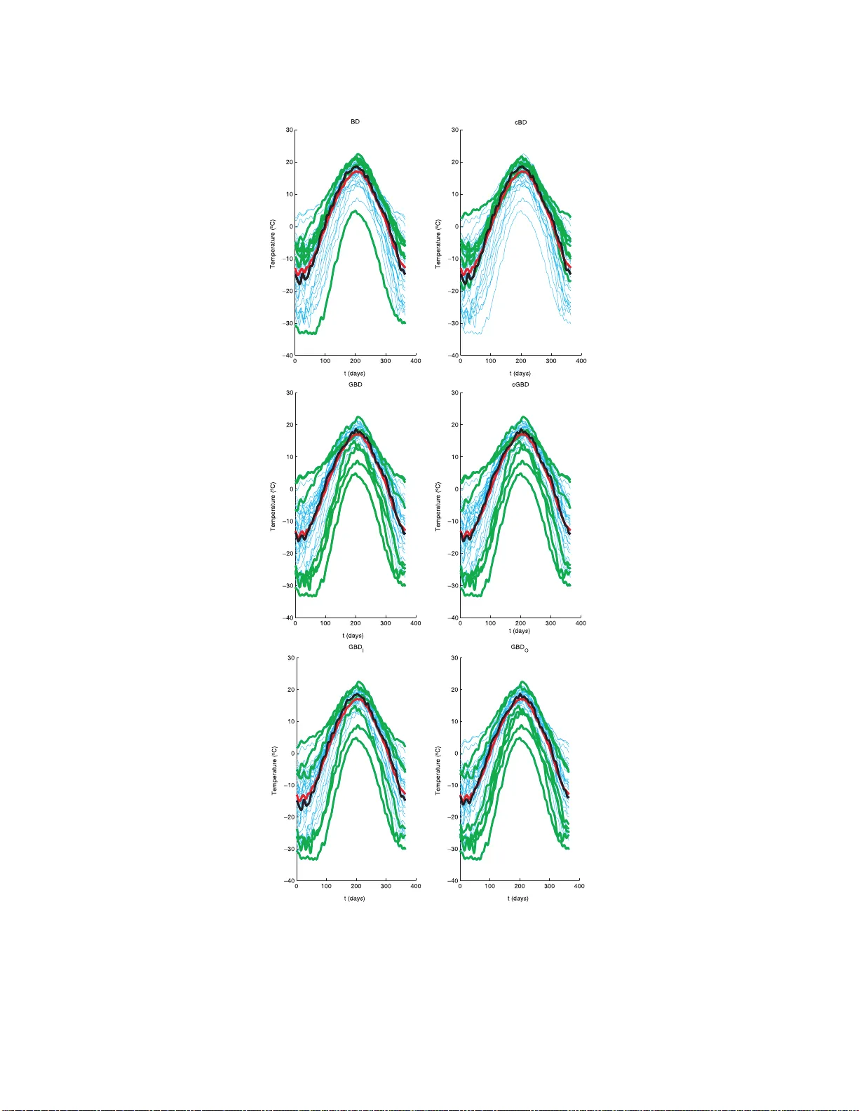
IMS Lecture Notes–Monograph Series Complex Datasets and In ve rse Problems: T omogra ph y , Net works and Beyond V ol. 54 (2007) 103–120 c  Institute of Mathematical Statistics, 2007 DOI: 10.1214/0749217 07000000085 F unction al analysis vi a e xtension s of the band d epth Sara L´ op ez-Pinta do 1 and Reb eck a Jornsten 2 , ∗ Universidad Pablo de Olavide and R utgers Universit y Abstract: The notion of data depth has long b een in use to obtain robust lo cation and scale estimates in a multiv ar i ate setting. The depth of an observ a- tion is a measure of its cen tralit y , wi th resp ect to a data set or a di s tribution. The data depths of a set of multiv ar iate observ ations translates to a center- out w ard or dering of the data. Thus, data depth pro vides a generalization of the median to a multiv ariate setting (the deepest observ ation), and can also be used to screen for extreme observ ation s or outliers (the observ ations with low data depth). Data depth has b een used i n the dev elopmen t of a wi de range of robust and non-parametric methods f or multiv ar iate data, s uc h as non-parametric tests of lo cation and s cale [ Li and Li u (2004)], multiv ariate rank-tests [ Liu and Singh (1993) ], non-parametric classification and clustering [Jornsten (2004)], and robust regression [ R ousseeu w and H ubert (1999)]. Many different notions of data depth ha v e b een developed f or mu ltiv ariate data. In contrast, data depth measures for functi onal data hav e only recently been proposed [F raiman and Muniz (1999) , L´ opez-Pintado and Romo (2006a)]. While the definitions of b oth of these data depth m easures are motiv ated by the functional asp ect of the data, the measures themselves are in fact inv ari- an t with r espect to permutations of the domain (i. e. the compact interv al on which the functions are defined). Thus, these measures are equally applicable to m ultiv ariate data where there i s no explicit ordering of the data dimensions. In this paper we explore s ome extensions of functional data depths, so as to tak e the ordering of the data dimensions into accoun t. 1. In tro duction In functional data a nalysis, each obser v atio n is a real function x i , i = 1 , . . . , n , de- fined on a commo n interv al in R . F unctional data is o bs erved in many disciplines, such as medicine (e.g. EEG traces), biolog y (e.g. gene expre ssion time co urse data), economics a nd engineer ing (e.g., financia l trends, chemical pro cesses). Many m ul- tiv ar ia te methods (e.g . ana lysis of v ariance, and cla ssification) hav e b een extended to functional data (see Ramsay a nd Silverman [2 2]). A bas ic building blo ck o f such statistical analyses is a lo catio n estimate, i.e. the mean cur ve for a group o f da ta ob jects, or data ob jects within a class. When analyzing functional data, outlier s ca n affect the lo cation estimates in many different wa ys, e.g. a ltering the shap e and/or magnitude of the mean c urve. Since measurements a re frequently noisy , statistical analysis may thus b e m uch impr ov ed b y the use of r obust lo cation estimates, s uch as ∗ Corresp onding author is funded by N SF Grant D M S-0306360 and EP A Star Grant RD- 83272101 -0. 1 Departamen to de Economia, Metodos Cuant itativ os e Historia economica, Uni v ersidad Pablo de Olav ide, Edif. n3-Jose M onino-3 planta Ctra de Utrera, K m. 1 41013 Sevilla, Spain, e-mail: sloppin@ upo.es 2 Departmen t of Statistics, Rutgers Universit y , Piscata w ay , NJ 07030, USA, e-mail : rebecka@ stat.rutge rs.edu AMS 2000 subje c t classific ations: 62G35, 62G30. Keywor ds and phr ases: data depth, functional data, band depth, r obust statistics. 103 104 S. L´ op e z-Pintado and R. Jornsten the median o r trimmed mean curve. Data depth provides the to ols for co nstructing these robust estimates . W e first review the concept of data depth in the m ultiv aria te setting, where data depth was intro duced to generaliz e order statistics , e.g. the median, to higher dimensions. Given a distribution function F in R d , a statistical depth assigns to each po int x a re al, no n- negative b ounded v alue D ( x | F ), which measures the centrality of x with resp e ct to the distr ibution F . Given a sample o f n obs e rv a tions X = { x 1 , . . . , x n } , we denote the sample version by D ( x | F n ) or D ( x | X ). D ( x | X ) is a measure o f the centrality of a p o int x with resp ect to the sample X (o r the empirical distribution function F n ). The p oint x ca n b e a sample obse rv a tion, o r constitute independent “ tes t data”. F or x = x i ∈ X , D ( x i | F n ) pr ovides a center-outw ard ordering of the s ample observ ations x 1 , . . . , x n . Many depth definitions have b een prop osed for mult iv a r iate da ta (e.g. Maha - lanobis [19], T ukey [26], Oja [2 0], Liu [12], Singh [25], F raiman and Melo che [3], V ardi and Zha ng [2 7] a nd Zuo [31 ]). T o illustra te the data depth principle and the v ar iety of de pth measures, we will br iefly r eview tw o very different notions of depth: the simplicial depth of Liu [12], and the L 1 depth of V ar di and Zhang [27] (a detailed discussion of the differe nt types of da ta depths ca n b e found in Liu, Parelius and Singh [14] and Zuo a nd Serfling [32]). T o compute the simplicial depth of a p oint x ∈ R d with res p e c t to the sa mple X = { x 1 , . . . , x n } , w e star t by pa rtitioning the sample into a set o f  n d +1  unique (d+1)-simplices. Cons ide r the tw o-dimensional case illustrated in Figure 1a. W e depict a s ubset of the  n 3  3-simplices (triangle s ) in R 2 defined by a s et of o b jects ( x 1 , x 2 , x 3 ) ∈ X . A p o int x is considered deep within the sample X if many simplices contain it, and vice versa. F ormally , the simplicial depth of a p oint x is defined as S D ( x | X ) =  n d + 1  − 1 X 1 ≤ i 1 2 is computationally intensiv e to w ork with since the nu mber o f unique bands grows at r ate  n J  . In addition, the band delimited by 3 data ob jects (Figure 2c) do es not provide the same intuition as the band delimited by 2 ob jects (Figur e 2a ). The shap e of the band delimited by J = 3 ob jects may differ substantially from the individual ob jects. Th us, if curve x is contained in band B ( x i 1 , x i 2 , x i 3 ), this do es not necess arily imply that x is similar to any of the ob jects x i 1 , x i 2 , x i 3 . When the curves are very irregular , the band depth can b e to o restrictive. F ew bands will fully contain a da ta ob ject. This will again r esult in to o many ties b etw een data ob jects, a nd a p o o rly defined cent er-outw ard ranking. A more flexible notio n of depth (the gener alize d band depth) was therefo r e pr op osed in L´ o pez -Pintado and Romo [16]. It is obtained by r e placing the indicator function in definition (2.2) by the pr op ortion o f time the c ur ve x is inside a co r resp onding band. Given the sample x 1 , . . . , x n , let for any curve x A ( x ; x i 1 , x i 2 , . . . , x i j ) =  t ∈ T : min r = i 1 ,...,i j x r ( t ) ≤ x ( t ) ≤ max r = i 1 ,...,i j x r ( t )  , j ≥ 2 , be the set of p oints in the interv al T wher e the function x is inside the band delimited by x i 1 , x i 2 , . . . , x i j . If λ is the Leb e sgue measure in R , λ ( A j ( x )) λ ( T ) is the prop ortion of time that x is inside the band. W e define (2.3) GS ( j ) n ( x | X ) =  n j  − 1 X 1 ≤ i 1 2 can b e ma de a t the exp ense of a n increased computationa l burden. 3.1. T he c orr e cte d (gener alize d) b and depth W e b egin by r evisiting the definition of a delimiting band. Ideally , we want each band to gather curves o f simila r shape ins ide it. T o achiev e this, we make the following adjustments to the definition of a band: If tw o curves cross, the band will be defined only where o ne of the curves is the upper cur ve and the o ther one is the lower curve. Hence, for each pair of curves that cro ss, there ar e tw o p o ssible bands (dep ending o n whic h curve is c o nsider the uppe r curve). W e will choo s e the longest of the tw o bands. The notions of c orr e cte d band depth and its g eneralized version are defined similarly to the band depth and the genera lized band depth, but re- defining the band as describ ed ab ove. W e first define the cor rected band depth ( cB D ). Let a ( i 1 , i 2 ) = { t : x i 2 − x i 1 ≥ 0 } and L i 1 ,i 2 = λ ( a ( i 1 ,i 2 )) λ ( T ) ( λ is the Leb esgue measure). B y exchanging the role s of the upper ( x i 1 ) and low er ( x i 2 ) curves we obtain L i 2 ,i 1 in a similar fa shion. W e define the corr ected band B c as B c = I { L i 1 ,i 2 ≥ 1 / 2 } B c ( x i 1 , x i 2 ) + I { L i 2 ,i 1 > 1 / 2 } B c ( x i 2 , x i 1 ) , where B c ( x i 1 , x i 2 ) = { ( t, y ) : t ∈ a ( i 1 , i 2 ) , x i 1 ( t ) ≤ y ≤ x i 2 ( t ) , } , and similar ly for B c ( x 2 , x 1 ). W e also form the cor rected graph G ( x ∗ ) as G ( x ∗ ) = { ( t, x ( t )) : t ∈ a ( i 1 , i 2 ) } , if L i 1 ,i 2 ≥ 1 / 2 , G ( x ∗ ) = { ( t, x ( t )) : t ∈ a ( i 2 , i 1 ) } , if L i 2 ,i 1 > 1 / 2 . Extensions of the b and depth 109 W e can now define the corrected band depth of a curve x with r esp ect to the sa mple X as (3.1) cB D ( x | X ) =  n 2  − 1 X 1 ≤ i 1 1 / 2 . Hence, the difference b etw een the c orr e ct e d (generalized) ba nd depth and the (g en- eralized) band depth is tha t the band is mo dified in order to cons ide r only the prop ortion of the domain wher e the delimiting curves define a contiguous r egion of non-zero width. 3.2. GB D I and G B D O —ac c ounti ng for c onse cutive b and excursions If a curve is only partia lly contained in a delimiting band, it may still share ma ny characteristics with the delimiting ob jects. Howev er, this simila rity ma y not b e optimally measur ed by the numb er of ex cursions outside the band, as with GB D , but per ha ps how these excursions present themselves. W e therefore pro po se tw o alternative definitions o f the gener a lized ba nd depth called GB D I and GB D O . W e pr op ose GB D I as a more conse r v a tive a lternative to GB D . W e r eplace λ ( A ( x ; x i 1 , x i 2 )) (the num ber o f t ∈ T where x ∈ B ( x i 1 , x i 2 )) in equation (2.3) by a measur e C I ( x ; x i 1 , x i 2 ), where C I ( x ; x i 1 , x i 2 ) = max t S  λ ( t S ) : min r = i 1 ,i 2 x r ( t ) ≤ x ( t ) ≤ max r = i 1 ,i 2 x r ( t ) , ∀ t ∈ t S  , where t S is a c omp act interval . That is , C I ( x ; x i 1 , x i 2 ) is the lo ngest co nsecutive stretch for which x is inside in the band delimited by x i 1 , x i 2 (C onsecutive Inside). Given sa mple functions x 1 , x 2 , . . . , x n , the GB D I of a curve x is (3.3) GB D I ( x | X ) =  n 2  − 1 X 1 ≤ i 1 x ( t ) or x ( t ) > max r = i 1 ,i 2 x r ( t ) , ∀ t ∈ t S  , and t S again denotes a compact set o n the interv al T . That is, C O ( x ; x i 1 , x i 2 ) is the longest contiguous region of the curve outside the delimiting ba nd (C onsecutive Outside). The GB D O of curve x with r esp ect to sample x 1 , . . . , x n is defined as (3.4) GB D O ( x | X ) =  n 2  − 1 X 1 ≤ i 1 0. Different v alues of k , c and µ change the shap e of the g enerated functions. F or exa mple, increasing µ and k , makes the curves smo other; wher eas, incr e asing c makes the curves more irre g ular. Mo del 6 is a mixture o f X i ( t ) = g ( t ) + e 1 i ( t ), 1 ≤ i ≤ n, with g ( t ) = 4 t and e i 1 ( t ) a g aussian sto chastic pro cess with zer o 114 S. L´ op e z-Pintado and R. Jornsten mean and cov ar ia nce function γ 1 ( s, t ) = exp {−| t − s | 2 } and Y i ( t ) = g ( t ) + e 2 i ( t ) , 1 ≤ i ≤ n, with e i 2 ( t ) a ga ussian pro cess with zero mean and cov a riance function γ 2 ( s, t ) = exp {−| t − s | 0 . 2 } . The contaminated Mo del 6 is Z i ( t ) = (1 − ε ) X i ( t )+ ε Y i ( t ), 1 ≤ i ≤ n, where ε is a Ber noulli v ariable B e ( q ) and q is a small contamination probability; thus, we c o ntaminate a sample of smo o th curves from X i ( t ) with more irregula r curves fro m Y i ( t ). W e ana lyze the p erfor mance of different notions of depth in terms of robustness. The no tions of depth consider ed are: the band depth with J = 2 and J = 3 ( B D 2 , B D 3 ), the generalized band depth ( GB D ), the corre cted version of the band depth and ge ne r alized band depth ( cB D , cGB D ), and the genera lized ba nd depths that acco unt for cons ecutive band excur sions, GB D I and GB D O . W e compare the mean and the α -tr immed mean, given by b µ n ( t ) = n P i =1 Y i ( t ) n and b m α n ( t ) = n − [ nα ] P i =1 Y ( i ) ( t ) n − [ nα ] , where Y (1) , Y (2) , . . . , Y ( n ) is the sample ordered from the deepes t to the most extreme (least dee p) curve and [ nα ] is the in teger part of nα. The rank- orders are computed using the re-sampling based depths. F or each mo del, we consider R = 200 repli- cations, each gener ating n = 150 cur ves, with contamination probability q = 0 . 1 and co nt amination constant M = 25 . The integrated error s (ev aluated at V = 30 equally spaced p oints in [0 , 1]) for each r eplication j are E I µ ( j ) = 1 V V X k =1 [ b µ n ( k /V ) − g ( k /V )] 2 and E I α D ( j ) = 1 V V X k =1 [ b m α n ( k /V ) − g ( k /V ) ] 2 , where D refers to one of the data depths ( B D 2 , B D 3 , cB D , GB D, cGB D , GB D I or GB D O ). All metho ds are applied to each simulated data set. Acros s simulated da ta sets we see a lot v ar iability since the contaminations are random. W e ther efore summarize the results as follows; (1) F or each mo deling scenar io and each simulated data set j , we compute the minimum in tegrated err or ac ross all metho ds E I α ∗ ( j ) = min D = B D 2 ,B D 3 ,cB D,GB D,cGB D,GB D I ,GB D O E I α D ( j ); (2) W e adjust the integrated error s by subtra cting the minimum v alue, such that the be s t metho d has adjusted integrated erro r 0, E AI α D ( j ) = E I α D ( j ) − E I α ∗ ( j ). W e summarize the simulation results in terms of the mea n and sta nda rd deviation of the adjusted integrated error s, E AI W e will first examine each simulation model se pa rately , and then discuss the ov erall r esults at the close of the section. Mo del 0 g enerates uncontaminated data. F ro m T a ble 1 we see that the mean is the b est estimate, as exp ected. The generalized ba nd depths ( GB D , cGB D , GB D I and GB D O ) p er form b etter than the band depths ( B D 2 , B D 3 and cB D ) in this setting, but all of the r obust e stimates p erform rea sonably well o n uncont aminated data. Some loss of estimation efficiency is unavoidable since a fixed tr imming factor α = 0 . 2 w as used. Sim ulations settings 1 through 3 corresp ond to simple co ntaminations, i.e. a po sitive or negative mea n o ffset, o r a partia l mean offset cont amination. In this Extensions of the b and depth 115 T a ble 1 Simulation r esults for t he seven mo deling sc enarios. Me an and standar d deviations of the adjuste d inte gr ate d err ors (subtr act ing the inte gr ate d err or of the winning metho d for e ach simulation), with R = 200 r eplic ations, q = 0 . 1 and α = 0 . 2 . M0 M1 M2 M3 M4 M5 M6 Mean 0.002 6.600 0.463 0.204 0.036 0.063 0.012 (0.003 ) (3.319) (0.606) (0.278) (0.027) (0.025) (0.012) B D 2 0.007 4.864 0.286 0.204 0.021 0.036 0. 008 (0.009) (3.832) (0.395) (0.278) (0.019) (0.028) (0.010) B D 3 0.007 3.916 0.163 0.053 0.012 0.014 0.005 (0.009) (3.189) (0.227) ( 0.119 ) (0.014) (0.018) ( 0.005) cB D 0.009 5.353 0.277 0.091 0.006 0.003 0.005 (0.012) (4.137) (0.365) (0.274) ( 0.011 ) (0. 008) (0 .010) GB D 0.005 0.085 0.005 0.050 0.047 0.074 0.013 (0.005) (0.286) (0.008) ( 0.074 ) (0.034) (0.034) (0.010) cGB D 0.004 0.117 0.005 0.048 0.046 0.074 0.013 (0.005) (0.381) (0.008) ( 0.075 ) (0.034) (0.033) (0.010) GB D I 0.005 0.260 0.007 0.055 0.043 0.043 0.003 (0.005) (0.619) (0.010) ( 0.072 ) (0.031) (0.026) ( 0.006) GB D O 0.005 0.001 0.003 0.060 0.049 0.083 0.022 (0.007) ( 0.003 ) (0.00 7) (0.0 90) (0.036) (0.037) (0.022) setting we ex p ect only marginal g ains fr om the use of sha pe sensitive or r estrictive depths such a s cB D a nd GB D I . On the o ther hand, the data is no isy so we exp ec t that cGB D and GB D O should p e r form well. F or the ca se of asymmetric contamination (Mo del 1 ), w e find that GB D O outp e r- forms the other metho ds. The trimming factor is α = 0 . 2, while the co nt amination probability is q = 0 . 1. Th us, for man y of the sim ulated data sets, s ome of the uncontaminated curves will b e trimmed. The band depths ( B D 2 , B D 3 and cB D ) all struggle in this setting. The uncontaminated curves frequently cross , leading to to o many ties in the rank- o rder. While the GB D, cGB D and GB D I per form muc h better than the band depths, they are not comp etitive with GB D O . The s ource of the pro blem lies in the a symmetry of the c o ntaminations, and that the magnitude outliers contribute to the computation o f the depth v alues o f all other o bserv ations (see Figure 6). Since GB D , c GB D a nd GB D I are more restr ictive than GB D O , these three depth measures trim more curves from the low er p ortion of the un- contaminated set than from the upper po rtion, crea ting a bias in the trimmed mean es timate. This suggests that p erhaps an iterative pro cedure , were outlier s are dropp ed one at a time and the data depths r e-estimated after each step, would per form b etter. As exp ected, when the contamination is symmetric (Mo del 2), GB D , cGB D and GB D I per form almos t as well as GB D O . The trimming of the uncon taminated data set is now mostly symmetric, and the trimmed mean estimates essentially unbiased. The band depths are not comp etitive. Mo del 3 generates data ob jects that have b een partially contaminated. This symmetric contamination is easily identified by GB D , cGB D , GB D I and GB D O . Sim ulation settings 4 through 6 can lo o sely be seen as shap e contaminations (Figure 6). Here, w e expe ct the cB D and GB D I to perfor m well, whereas the per formances of the les s restrictive GB D , cGB D and GB D O may deterior ate. Indeed, fo r Mo del 4 (p eak contamination), cB D is the b est metho d, fo llow ed by B D 3 and B D 2. cB D improves on the band depths since the band co rrection accounts for curves that cr oss. The generalized band depths ( GB D, cGB D, GB D I and GB D O ) do not p erfor m well in this setting, even o ccas ionally resulting in an int egrated err or exceeding that of the mea n. 116 S. L´ op e z-Pintado and R. Jornsten Fig 6 . Curves gener ate d fr om Mo del 1: asymmetric c ontamina tion (top left ), M o del 2: sym- metric c ontamina tion (top right), Mo del 3: p artial c ontamination (midd le left), Mo del 4: p e aks c ontamina tion (midd le right), Mo del 5: uniform c ontamination (b ottom lef t ), Mo del 6: shap e c on- tamination (bo ttom rig ht). The mea n curve is depicte d in r e d, and t he trimme d me an in gr e en in al l c ases. Extensions of the b and depth 117 In Mo del 5 we allow for m ultiple co nt aminations of each cur ve. The p erfo rmance of the GB D , cGB D and GB D O deteriorates since these shor t excursions are not recognized a s a contamination. GB D I per forms a little b etter, since the unifor m contamination leads to the co nt aminated curves residing in the bands for only short consecutive stretches. Still, GB D I is not co mpe titive with the band depths (though b etter than the mean). The bes t metho d is ag ain the cB D , fo llow ed by the computationally exp ensive B D 3 . In Mo del 6 (shap e contamination), a set of smo oth curves ar e co ntaminated by a set of irreg ular curves. W e expect the shap e sensitive methods (band depths, GB D I ) to excel in this setting. Indeed, the GB D I is the bes t metho d, follow ed closely b y cB D a nd B D 3 . Ag ain, the less restrictive depths ( GB D, cGB D and GB D O ) do not p erfor m w ell in this setting. In the first three simulations (Mo dels 1 through 3), the genera lized band depths, with GB D O in the lead, outp erfor m the band depths. The contaminations in Mo dels 1 thro ugh 3 are es sentially mag nitude outliers, and p er sistent acr o ss the compact int erv al T . In simulations fr o m Mo dels 4 through 6, the contaminations a re more subtle (ra ndom p eaks, or a different cov aria nce str ucture). In such settings, the less restrictive data depths, tha t discar d sho rt excurs io ns as non-infor ma tive, p erfor m po orly . The band depths, with the co r rected band depth in the lead, as w ell a s the GB D I , per form well in this s etting. It is cle ar then, that one depth ca nnot b e defined as the “ be st” a cross all pos s ible scenarios . Ther efore, in practise one nee ds to consider the type of contaminations to screen against. W e recommend that several depths a re applied to each da ta set, and the o utliers identified by ea ch depth meas ure exa mined gr aphically . F rom the ab ov e simulation r esults we see that GB D O and cB D a re tw o candidate measur e s that are fast and e asy to compute, and w ould highlight different structures in the data. T o illustr ate the scr eening pr op erties of the depth measures, we apply six no- tions of depth to a data set co nsisting of the daily temper ature in 35 differ- ent Ca nadian w eather stations for one year (Ramsay and Silverman [22]). The original data was smo othed using a F ourier basis with sixty five elements. In Figure 7 we show the mean and the median (deep est) curve identified by the B D , cB D , GB D, cGB D, GB D I and GB D O . In addition, in e a ch figur e we high- light the 20 % least deep curves in green (wide lines). F r om the ab ove dis cussion, and the definitio ns in Sections 2 a nd 3 , we know that GB D , cGB D and GB D O are the leas t restrictive depths. These depths will larg e ly iden tify mag nitude outliers as the least deep. In Figure 7 we see that this is indeed the c ase for the temp erature data set. In co nt rast, B D , cB D and GB D I are the most res trictive, and will iden- tify shap e outliers . T emper ature pr ofiles that are flatter than the rest of the data, or irreg ular with large, lo cal fluctuations, ar e ident ified by these depths. 6. Discussion W e introduce several extension of the band depth for functional da ta. These new notions of depth a ccount for the explicit ordering of the da ta dimensions inherent to functional data. W e find that a simple altera tion of the definition of a delimiting band, a band correc tio n, can improve on the previo usly pr op osed band depth. In addition, a differe ntial treatmen t o f band excursions tha t a re co nsecutive versus isolated, can b o ost the p erformance of the g eneralized band depth. While tw o of our pro po sed extensions , the cor rected band depth cB D and the GB D O , improve o n the band depth and the genera lized band depth res pe ctively , we 118 S. L´ op e z-Pintado and R. Jornsten Fig 7 . Comp arison of the 6 notions of depth. In ea ch figur e , we depict the me an curve (r e d), and me dian curve (black). The 20% le ast de ep curves ar e plotte d in gr e e n (wide lines), wher ea s the 80% most c entr al curves ar e depicte d in cyan (thin lines). T op p anel: B D and cB D . Midd le p anel: GB D and cGB D . Bottom p anel: GB D I and GB D O . Extensions of the b and depth 119 cannot identify a “ b est” data depth for functiona l data that uniformly dominates the o ther measures a cross all forms of co nt amination. The GB D O is the mo st comp etitive in simple contamination scena rios (magnitude outliers), wher eas the cB D is more comp e titiv e when the samples are contaminated b y cur ves of a different structure or shap e. Our reco mmendation is that a set of data depths are used to screen the data for contaminations. A gr a phical examina tion of the data set can elucidate the po tential outliers or extreme obser v atio ns. One must make a case-by-case decision as to which functional shap es co ns titute outliers in a par ticular data set. W e pro p o se a fast and simple re-sampling based data depth ca lculation pro c e- dure. The ra nk -orders induced by the re- sampling bas ed metho d closely agr ee with the rank- orders induced by the full data. With the computationally efficient re- sampling based metho d, the ne w notions of depth can b e us ed as building blo cks in non-par ametric functional analysis such as clus ter ing and classifica tio n. Ac kno wl edgments. The authors w ould like to thank the reviewer fo r many insightful comments a nd helpful sugg e stions. R. Jor nsten is partia lly supp orted by NSF Gra nt DMS-03 0636 0 and EP A Star Grant RD-832 72101 -0. The work for this pap er was conducted while S. L´ opez-P intado w as a p ostdo c- toral resea rcher at Rutgers Universit y , Department of Sta tistics. References [1] Arcones, M. A. and Gin ´ e, E. (1 993). Limit theore ms for U-pro ces ses. Ann. Pr ob ab. 21 1494 –154 2. MR1 2354 2 6 [2] Bro wn, B. and Hettmansperger, T. (1989 ). The affine inv ariant biv a riate version of the sign test. J. R oy. St atist. So c. S er. B 51 117–12 5. MR09849 98 [3] Fraiman, R. and Meloche, J. (199 9). Multiv ar iate L-e s timation. T est 8 255–3 17. MR1748 275 [4] Fraiman, R. an d Mu n iz, G. (2001). T rimmed means for functional data . T est 10 419– 440. MR1 8 8114 9 [5] Gho sh , A. K. and Chaudhuri, P. (200 5). On data depth and distribution- free dis c riminant analy s is using separating surfaces. Bernoul li 11 1. MR21214 52 [6] Hettmansperger, T. and Oja, H. (199 4 ). Affine inv aria nt m ultiv aria te m ultisample sig n tests. J. R oy. Statist. So c. Ser. B 56 23 5–249 . MR1 25781 0 [7] Inselberg, A. (1 9 81). N-dimensional graphics , Part I-lines and hyperplanes . In IBM LASC, T echnical Rep ort, G320-27 111. [8] Inselberg, A. (1985). The plane paralle l co ordinates . Invited pap er. Visual Computer 1 69–91. [9] Inselberg, A . , Reif, M. and Chomut, T. (19 87). Conv exit y algo rithms in parallel co ordinates . Journal of ACM 34 765– 801. MR0913 842 [10] Jo rn sten, R. (200 4). Clustering a nd classifica tion via the L1 data de pth. J. Multivariate Anal. 90 67 – 89. MR20649 37 [11] L i, J. and Liu, R. (20 04). New nonpar ametric tests of multiv a riate lo ca tions and scales using data depth. Statist. Sci. 19 68 6–69 6 . MR2 18559 0 [12] L iu , R. (1990). On a no tion of da ta depth bas ed on ra ndo m simplices . Ann. Statist. 18 40 5–414 . MR1 04140 0 120 S. L´ op e z-Pintado and R. Jornsten [13] L iu , R. (1995). Control charts for m ultiv ar ia te pro c e sses. J . Amer. Statist. Asso c. 90 13 80–1 388. MR1379 481 [14] L iu , R., P arelius, J. M. and Singh, K. (19 99). Multiv a riate analysis by data depth: Descriptive sta tistics, gr aphics and inference. Ann. Statist. 27 783–8 58. MR1724 033 [15] L iu , R. and Singh, K. (199 3). A q uality index bas ed on data depth and m ultiv ar iate rank test. J . Amer. S tatist. Asso c. 88 2 57–2 6 0. MR12124 89 [16] L ´ opez-Pint ado, S. and Romo, J. (200 6a). Depth-based inference for func- tional data. Comput. St atist. Data Anal. In press. [17] L ´ opez-Pint ado, S. and Romo, J. (2006b). Depth-based c la ssification for functional data. In Data Depth: R obust Multivariate Analy sis, Computational Ge ometry and Applic ations . D imacs Series in Discr ete Mathematics and The- or etic al Computer Scienc e 72 (R. Y. Liu, R. Serfling and D. L. So uv aine, eds.). Amer. Math. So c., P rovidence, RI. In press . [18] L ´ opez-Pint ado, S. and Romo, J. (2006 c). On the concept of depth for functional data. J. Amer. Statist. A sso c. Submitted. Second revisio n. [19] Maha l anobis, P. C. (193 6). On the generalize d distance in statis tics . Pr o c. Nat. A c ad. Sci. India 12 49–5 5. [20] Oja, H. (1983). Descr iptive statistics for multiv ar iate distr ibutions. Statist . Pr ob ab. L et t. 1 327– 332. MR072 1446 [21] P ollard, D. (198 4). Conver genc e of St o chastic Pr o c esses . Springer, New Y ork . MR076298 4 [22] Ramsa y, J. O. and Sil verman, B. W. (2005). F un ctional Data Analy sis , 2nd ed. Springer , New Y ork . MR21 6899 3 [23] Rousseeuw, P. and Huber t, M. (199 9). Regression depth (with discussion). J. Amer. Statist. Asso c. 4 388– 433. MR170 2314 [24] S erfling, R. J. (1980 ). Appr oximation The or ems of Mathematic al Statistics . Wiley , New Y or k. MR05951 65 [25] S ingh, K. (19 91). A notion of ma jority depth. Unpublished do cument. [26] Tukey, J. (1 975). Mathema tics and pictur ing data . Pr o c e e dings of the 1975 International Congr ess of Mathematics 2 523 – 531. MR0 4269 89 [27] V ardi, Y. and Zhang, C.-H. (200 1). The multiv aria te L1-median a nd ass o- ciated data depth. Pr o c. Nat. A c ad . Sci. USA 97 14 23–1 426. MR174 0 461 [28] W egman, E. (1990). Hyp erdimensional data ana lysis using par allel co ordi- nates. J. Amer. Statist. Asso c. 85 664 –675. [29] Wood, A. T. A. and Chan, G . (1994 ). Simu lation of stationary gaussia n pro cesses in C [0 , 1 ]. J. Comput. Gr aph. Statist. 3 409–4 32. MR13 2305 0 [30] Y eh, A. and Singh, K. (199 7). Balanc e d confidence sets based on the T ukey depth. J. R oy. Statist. S o c. Ser. B 3 639 –652. MR145 2031 [31] Z uo, Y . (2003 ). Pro jection based depth functions and as so ciated medians. Ann. Statist. 31 14 60–1 490. MR20128 2 2 [32] Z uo, Y . and Serfling, R. (2000 ). Genera l notions o f s tatistical depth func- tion. Ann. Statist. 28 46 1–48 2 . MR1790 005