Statistical inverse problems in active network tomography

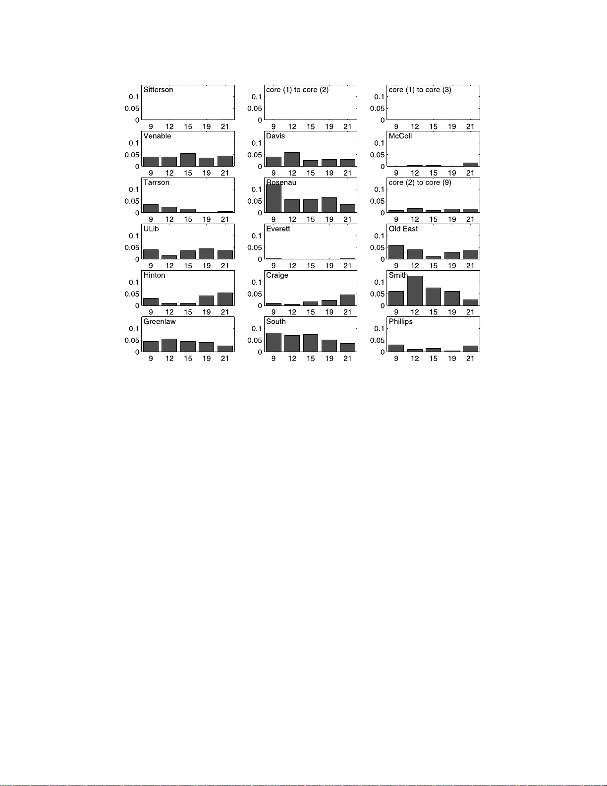
IMS Lecture Notes–Monograph Series Complex Datasets and In ve rse Problems: T omogra ph y , Net works and Beyond V ol. 54 (2007) 24–44 In the Public Domain DOI: 10.1214/0749217 07000000049 Statistic al in v erse proble ms in activ e net w ork tomograph y Earl La wrence 1 , ∗ , George Mic hailidis 2 , ∗ and Vija y an N. Nair 2 , ∗ L os Alamos N ati onal L ab or atory and University of Mi chigan Abstract: Th e analysis of computer and communica tion netw orks gives rise to some interesting inv er se problems. This pap er is concerned wi th activ e netw ork tomograph y where the goal i s to recov er information ab out quality-of-service (QoS) par ameters at the link l ev el from aggregate data measured on end-to- end net w ork paths. The estimation and monitoring of Q oS parameters, suc h as loss rates and delays, are of considerable interest to netw ork engineers and In ternet service providers. The paper provides a review of the inv erse problems and recen t research on inference for loss rates and delay distri butions. Some new results on parametric inf erence f or dela y distributions are als o dev eloped. In addition, a real appli cation on In ternet telephon y is discussed. 1. The in v erse probl ems Consider a top ology with a tree structur e de fined as fo llows: T = {V , E } has a set o f no des V and a s et of link s or edges E . Figure 1 shows t wo exa mples, a simple tw o-layer symmetric binary tree on the left and a more general four - lay er tree on the right. Each member of E is a directed link n umbered after the node at its terminus. V includes a (single) ro ot no de 0 , a se t of rece iver or destination no des R , and a set of internal no des I . The int ernal no des hav e a single inco ming link and at least tw o outgo ing links (c hildren). The receiver no des have a single incoming link but no c hildren. F or the tree on the right panel of Figure 1, R = { 2 , 3 , 6 , 8 , 9 , 10 , 1 1 , 12 , 13 , 14 , 15 } and I = { 1 , 4 , 5 , 7 } . All tra nsmissions are sent fro m the ro o t (or sour ce) no de to one or mo re of the receiver no des. This gener ates indep endent obse r v a tions X k at a ll links alo ng the paths to those r eceiver no des. Let X denote this set of measurements. These data are not directly observ able; rather we can collect only end-to-end data at the receiver no des: Y r = f ( X ) for r ∈ R . The statistical in verse problem is to r e c onstruct the distributions of the link-level X k s fr om these p ath-level m e asur ements . Examples of f ( · ) are: f ( X ) = P k ∈P (0 ,r ) X k , f ( X ) = Q k ∈P (0 ,r ) X k , and f ( X ) = min k ∈P (0 ,r ) X k , and f ( X ) = max k ∈P (0 ,r ) X k , wher e P (0 , r ) is the path betw een the ro ot no de 0 and the rece iver no de r . In this pap er, we will b e conce r ned only with the first tw o ca ses of f ( · ) ab ove. T o understand the statistical issues a nd challenges involv ed, let us examine some simple examples. ∗ The research was supported in part by NSF Grants CCR-0325571, DM S-0204247 and DMS- 0505535. 1 Statistical Sciences Group, Los Alamos National Labor atory , Los Alamos NM 87545, USA, e-mail: earl@lanl.gov 2 Departmen t of Statistics, Universit y of Michigan , Ann Ar bor MI 48109, USA, e-mail: gmichail @umich.edu ; vnn@umich .edu AMS 2000 subje c t classific ations: 62F10, 60G05, 62P30. Keywor ds and phr ases: Netw ork tomograph y, internet, inv erse problems, monitoring, nonlinear least squares. 24 Inverse pr oblems in net work tomo gr aphy 25 Fig 1 . Examples of tre e network top olo gies. A binary two-layer tr e e is shown on the left p anel and a gener al f our-layer tr e e on the rig ht p anel. The p ath lengths fr om the r o ot to no des b elonging to the same layer ar e the same. Example 1. Consider the tw o-lay er binary tr ee on the left panel of Figur e 1 , a nd suppo se the X k are binary with P ( X k = 1) = α k , k = 1 , 2 , 3 for the three links. F urther, the ro ot no de se nds transmiss ions to the rece iver no de s one at a time . T ak e f ( a, b ) = ab . Then, the observed data are Y 2 j = X 1 j X 2 j for tra nsmission j and Y 3 m = X 1 m X 3 m for tra nsmission m . They are indep endent Bernoulli with prob- abilities α 1 α 2 and α 1 α 3 , re sp ectively . Supp ose we send M transmiss ions to receiver no de 2 and N transmissio ns to r eceiver no de 3 . Let M 1 and N 1 be the resp ec tive nu mber of “ones” . Then, M 1 and N 1 are independent binomial ra ndo m v ariables with success probabilities α 1 α 2 and α 1 α 3 . F rom these data, we can estimate only α 1 α 2 and α 1 α 3 . The individual link-level par ameters α 1 , α 2 and α 3 cannot b e fully recov ered. Example 2 . T a ke the same tw o-lay er binary tree with bina ry outcomes with f ( a, b ) = ab a s ab ov e. B ut now the ro ot no de sends transmissions to re c eiver node s 2 and 3 simultane ously . In other words, the m -th transmission gener ates random v ar iables X 1 m , X 2 m and X 3 m on all o f the links. W e obs erve Y 2 m = X 1 m X 2 m and Y 3 m = X 1 m X 3 m . The distinction fro m E x ample 1 is that the X 1 m is c om- mon to both Y 2 m and Y 3 m . Now, each transmiss ion ha s 4 p oss ible outcomes: (1 , 1) , (1 , 0) , (0 , 1) , (0 , 0 ) dep ending on whether the trans mis sion reaches none, one, o r b o th of the rece iver no des. If we se nd N such transmissio ns to no des 2 and 3 simultaneously , the re s ult is a multinomial ex pe r iment with pr obabilities α 1 α 2 , α 1 (1 − α 2 ), (1 − α 1 ) α 2 , and (1 − α 1 )(1 − α 2 ) cor resp onding to the four outco mes. Let N ( i, j ) denote the num ber of even ts with outcome ( i, j ). Then, E [ N (1 , 1)] = α 1 α 2 α 3 , E [ N (1 , 1) + N (1 , 0)] = α 1 α 2 , a nd E [ N (1 , 1) + N (0 , 1)] = α 1 α 3 . It is eas y to see that we can estimate all the three link- le vel para meters from thes e mea sure- men ts. Thus, the da ta transmissio n scheme plays an impo rtant ro le in this type o f 26 E. L awr enc e, G. Michailidis and V. N. Nair inv erse problems . Example 3. Again w e have a tw o -lay er binary tree but now f ( a, b ) = a + b . Then Y 2 = X 1 + X 2 and Y 3 = X 1 + X 3 . Let F k be the distribution of the link-le vel random v a riables X k ∈ R , for k = 1 , 2 , 3 . Assume, as in Example 2, that the ro ot no de sends transmissions simult ane ously to b o th receivers. In this ca se, even with simultaneous transmissio n to b oth r e ceivers, the link-level parameter s a re not alwa ys ide ntifiable. Just tak e X k to b e indep endent Normal( µ k , 1) , k = 1 , 2 , 3. Then Y 2 and Y 3 are biv ar iate nor mal with mea n µ 1 + µ 2 and µ 1 + µ 3 , v ariance 2 and correla tion 1. One can see that the individual µ k cannot b e r ecov ered from the joint distribution of Y 2 and Y 3 . Additional assumptions on the distribution are needed in order to so lve the inv erse pro blem. W e will revisit this issue. Example 4. Consider now the more general tree on the rig ht panel of Figure 1. Again, we s end tra nsmissions to all of the receiver no des simultaneously . If the r an- dom v ariables are binar y and f ( x 1 , . . . , x p ) = Q p j =1 x j , all the link-level parameters are identifiable. The same is tr ue fo r a general X k with f ( x 1 , . . . , x p ) = P p j =1 x j under suitable conditions on the distribution of the X k (as discussed later in the pap er). Howev er, it may b e “ exp ensive” to send transmissio ns to all r eceiver no des simult aneously . Instea d, can we schedule tr ansmissions to some judicious s ubsets of the rec eiver no des a t a time and co mbine the information appropria tely to estimate all the link-level parameters ? It is clea r fr o m Exa mple 1 that it is not enoug h to send trans mis s ions to one receiver no de a t a time. How sho uld the transmissio n scheme be desig ned in or der to estimate a ll the par a meters? Are there so me “go o d” schemes (accor ding to some appro priate criteria)? These ex amples are simple instances of issues that arise in the context of ana- lyzing computer and communications ne tw orks and are collectively r eferred to as active network tomo gr aphy. In the next section, we will describ e the netw ork ap- plication and the need for e s timating q ua lity-of-service (QoS) par ameters such as loss rates and de lays. Sec tio n 3 provides a n o verview of recent results in the lit- erature on the design of transmiss ion exp eriments and inference for loss r ates a nd discrete delay distributions. A rea l a pplica tion on data collected from the c a mpus net work at the Universit y of North Carolina, Chap el Hill is used to illus trate some of the results. Section 4 dev elops some new results on parametric inference for delay distributions. 2. Activ e net w ork tomograph y The ar ea of net work tomog raphy orig inated with the pioneering work of V ar di [14] where the term was first intro duced. His work dealt with another type o f in- verse problem r elating to o rigin-destinatio n (OD) traffic matr ix estimation. The OD informa tion is impor tant in netw ork management, ca pacity planning, and pro - visioning. In this pro blem, one is in terested in estimating the intensities of traffic flowing b etw een the orig in-destination pa irs in the net w ork. Ho wev er, we cannot collect these data dir ectly; ra ther, one places equipment at the individual no des (routers/s witches) and collects aggr e gate da ta o n a ll tr affic flowing through the no des i ∈ V . The go al is to re cov er distributions of orig in- destination tra ffic be- t ween all pa irs of no des in the net work. There has b een c o nsiderable work in this area, and a summar y of the developmen ts ca n be found in [3]. Activ e netw o rk tomography , o n the other hand, is concerned with the “opp osite” problem of estimating link-level informatio n from end-to-end data. One sends test Inverse pr oblems in net work tomo gr aphy 27 prob es (pa ckets) (active pr obing) fro m a source to one or more r eceiver no des on the per iphery of the netw o rk and gets end-to -end path- le vel da ta on losses a nd delays. One then has to solve the inv erse pro blem o f reconstruc ting link-level los s a nd delay information from the end-to-end data. The sp ecific goa l is to estimate QoS parameters such as loss ra tes a nd delays at the link level. The r eason for probing the netw ork from the o utside is that Internet servic e pr oviders o r other interested parties often do not hav e acces s to the internal node s of the netw ork (which may be owned by a third party). Nevertheless, they hav e to assess Qo S o f the links ov er which they ar e providing service. Active tomography offers a co nv enien t approach by pro bing the net work from no des lo cated on the p er iphery . The probing and data collection a re done with dedica ted instruments at the ro ot no de and receiver no des. These packets can b e sen t to one receiver a t a time (unica st transmission scheme) or to a sp ecified s ubset of receivers (multicast s cheme). Some net works hav e tur ned off the multicast sch eme for s ecurity reaso ns. In this case, one sends unicast pack ets to several receivers spaced close ly in time with the go al of trying to mimic the m ulticast scheme. What caus es losses a nd delays of pack ets over the net work? When a pack et arrives at a no de, it joins a q ueue o f incoming pack ets. If the buffer is full, the pack et is dropped, i.e., lo st. Depending on the proto co l, the pack et may or may not be resent. Pack ets also encounter delays alo ng the path, prima rily due to the queueing pro cess a b ov e. In the case of losses, the binar y outcome X k = 0 or 1 indicates whether the pa ck et is lost (dro pped) or not. In ter ms of the examples in Section 1, f ( x 1 , . . . , x k ) = Q k x k , a nd the end-to-end loss Y = Q k ∈P (0 ,r ) X k = 1 if the pa ck et transmitted along the path P (0 , r ) reached the receiver no de r and zero o ther wise. F or delays, f ( x 1 , . . . , x K ) = P k x k , and the end-to- end o bs erv a tion is Y = P k ∈P (0 ,r ) X k , the path-level delay . The physical topolo gy of a net work is usually complicated. But the log ical top ol- ogy with a single s o urce no de can o ften b e repres ented as a tree. F or example, the left panel o f Figure 2 shows the ph ysical top ology of a s ubnet work at the campus of the Universit y o f North Caro lina at Cha p el Hill. The right panel shows the cor- resp onding logical top olog y , which is a tree with a dire cted flow. W e will r evisit this netw ork later in the pap er. It is po ssible to deal with top ologies with multiple sources, o ther kinds of tra nsmission schemes (t w o-wa y flows), and so on. But fo r simplicity , we will res trict attent ion to the tr e e s tr uctures in this pa per . Fig 2 . L eft p anel: Schematic of the UNC network; R ight p anel: Lo g ic al top olo gy of the UNC network. 28 E. L awr enc e, G. Michailidis and V. N. Nair 3. Literature review of loss and discrete del a y inference Most of the r e sults in the literature on active tomography hav e b een developed under the assumption that the lo ss rates and delay dis tributions ar e tempo rally homogeneous a nd a re indep endent across links. W e will also use this framework. The assumption of temp oral homog eneity is r easonable as the probing exp eriments are done within the order of minutes. The assumption of indep endence acro ss links is les s likely to hold. How ever, the nature of the dep endence will v ar y from netw ork to netw ork, a nd it is difficult to obtain general results. 3.1. Design of pr obing exp eriments W e noted in E xample 1 that the link-level parameters are not identifi able under the unicast tr ansmission sch eme (sending pr o b es to one receiver a t a time). The m ulticast scheme, which sends pac kers to al l the receivers in the netw ork sim ultane- ously , address es this problem for loss ra tes and, under s ome additiona l conditions, for delay distributions as well. How ev er, this scheme has a n um be r of drawbacks. It creates mo re traffic than necessary fo r estimating the link-level para meters. Also, the data generated are very high-dimensional. F or example, in a binary symmetric tree with L lay ers, there are R = 2 L − 1 rece iver no des. A multicast scheme for measuring loss r a tes results in a multinomial exp er iment with 2 R po ssible outco mes. This is a la rge nu mber even for mo der ately sized trees. The most imp orta nt drawback, how ev er, is that it is inflexible a nd do es not allow in vestigation of subnetw orks using different intensities and at different times. In pr actice, o ne may want to prob e sensitive parts of the net work as lig ht ly as nec essary to av oid dis turbance. So there is a need for more flexible probing ex pe r iments. As p ointed out in E x ample 4, this ra ises interesting issues on how to design the probing exp er imen ts. A clas s of flexible pr obing exp er iment s, calle d flexic ast e x pe r iments, were in- tro duced and studied in Xi et al. [17] and Lawrence et al. [8]. This co nsists of a combination of s chemes for different v alues of k with each s cheme aimed a t study- ing a subnetw ork. How ev er, each of the s cheme b y itself will not necessarily allow us to estimate the link-level par ameters o f that subnet work. The data hav e to be combined a c r oss the v ar ious k-cast schemes to estimate the link-level pa rameters. T o illustra te the idea s, consider the netw ork o n the r ight pa nel in Figure 1. The m ulticast scheme sends prob es sim ultaneously to {h 2 , 3 , 6 , 8 , 9 , 1 0 , 11 , 12 , 13 , 14 , 15 i} . Two p os sible flexicast exp eriments a re: (1) {h 2 , 3 i , h 6 , 12 i , h 13 , 14 i , h 8 , 1 5 i , h 9 , 10 i , h 11 i} and (2) {h 2 , 3 i , h 6 i , h 12 , 1 3 , 14 , 1 5 i , h 8 , 9 , 10 , 11 i} . The former co nsists of only bicas t (t wo rec e iver no des at a time) a nd unicast schemes. Intuitiv ely , the latter scheme app ea rs to mo re “efficient” but we will se e shortly that it do es not allow one to estimate all the link-le vel parameter s. A full m ulticast scheme for this tree will result in 11- tuples o r 1 1 -dimensional data. The first flexica s t exper iment using pair s a nd singletons can cov er the whole tree with five pair s a nd one singleton. The re s ulting da ta are considera bly le ss complex in terms of pro cessing and co mputatio ns for inference. This adv antage is particularly imp ortant for trees with many layers. Inverse pr oblems in net work tomo gr aphy 29 Of course, not all flexicast exp er iments will per mit estimation of the link-level parameters . T o discuss the technical issues asso cia ted with the identifiabilit y prob- lem, cons ider first the no tion of a splitting no de. F o r a k - c ast scheme, an internal no de is a splitting no de if the scheme splits at that no de. F o r ex ample, for the tree on the rig ht pane l of Figure 1, the bicast scheme {h 6 , 12 i} splits at no de 4 . Xi et al. [1 7] show ed tha t the following conditions are necessa ry and sufficient for iden- tifiabilit y of link- le vel lo ss r ates: (a) all rece iver no des a re cov ered; and (b) every int ernal no de in the tree is a splitting no de for some k-ca st scheme in the flexicast exp eriment. Lawrence et al. [8] studied the delay problem and show ed that the same conditions are also necessary and sufficient for es tima ting delay distributions provided the distributions are discr ete. The case where the delay distributions are not discrete is discussed in the next sectio n. Consider a g ain the fle x icast schemes in equatio ns (1) a nd (2) for the tree on the right panel in Figur e 1. The first one base d on a colle c tion of bic a st and unicas t schemes satisfies the conditions . F o r the seco nd one, none of the k- cast schemes split at no de 4. There a re many flexicast exp eriments that sa tisfy the identifiabilit y require ments, and the c hoice among these ha s to be based on other criteria. Exper iments based on just bicast and unicasts hav e minimal data complexity – just 1- and 2-dimensio nal outcomes. How ever, these provide infor mation on just first and second-o rder de- pendenc ie s and will be less efficient (in a s tatistical sense) to k-cast schemes with higher v a lues of k . In particular , the full mulitcast s cheme will b e mos t efficient in this sense. So the overall ch oice of the flexicast exp eriment has to b e a compromise betw een statistical efficiency and flexibility including the a bility to adapt ov er time to acco mmo da te changes in netw ork conditions. 3.2. Infer enc e for loss r ates Inference for lo ss rates was fir s t studied in C´ aceres et al. [2 ] for the multicast s cheme. A recent, up-to- da te list of references can b e found in Xi et al. [17] who develop ed MLEs based o n the EM alg orithm for flexicas t exp eriments. W e provide next a brief review of these re s ults. Each k -cast scheme in a flex ic ast exp eriment is a k -dimensiona l mult inomial ex- per iment. Sp ecifically , each outcome is o f the form { Z r 1 , . . . , Z r k } whe r e Z r j = 1 or 0 dep ending on whether the prob e reached r e ceiver no de r j or not. Let N ( r 1 ,...,r k ) denote the num ber of o utcomes co rresp onding to this event , and let γ ( r 1 ,...,r k ) be the probability o f this even t. Then the log -likelihoo d for the k -cast scheme is prop or - tional to γ ( r 1 ,...,r k ) log( N ( r 1 ,...,r k ) ). The ov erall log-likeliho o d is just the s um of the log-likeliho o ds for these individual exp eriments. Ho wev er, the γ ( r 1 ,...,r k ) are co mpli- cated functions of α k , the link-level loss rates, s o one ha s to use numerical metho ds to obtain the MLE s. The EM algorithm is a natural appr oach for co mputing the MLE s and has b een used extensively in netw ork tomogra ph y applica tio ns (see [3, 5 , 16]). The structure of the EM-alg orithm for general flex ic a st exp er iments was develop ed in Xi et al. [17]. While the E -step c a n b e complex for arbitr a ry collections of k -ca st schemes, it simplifies for flexicast ex pe r iments comprised of bicast and unicast schemes as seen below. Let s b be the splitting no de for bicas t pair b = h i b , j b i . Then, π (0 , s b ), π ( s b , i b ) and π ( s b , j b ), the three path probabilities fo r this bicast pa ir are pro ducts of the α k . Starting with an initial v a lue ~ α (0) let ~ α ( k ) be the v alue after the k -th iteration. Then, we can write the ( k + 1)-th itera tio n of the E-s tep as follows: 30 E. L awr enc e, G. Michailidis and V. N. Nair E-step: 1. F or ea ch bicast pair: (a) Use ~ α ( k ) to obta in the up dated pa th probabilities π ( k ) (0 , s b ), π ( k ) ( s b , i b ), π ( k ) ( s b , j b ) and γ b ( k ) 00 . (b) F or each no de ℓ ∈ P (0 , s b ) ∪ P ( s b , i b ) ∪ P ( s b , j b ), compute V ( k +1) ℓ,b = E ~ α ( k ) [ V ℓ | N b ], where N b = { N b 00 , N b 01 , N b 10 , N b 11 } are the collected c o unts of the four po ssible outcomes, as follows. F or no de ℓ ∈ P (0 , s b ), V ( k +1) ℓ,b = N b − N b 00 1 − α ( k ) ℓ γ b ( k ) 00 . F or link ℓ ∈ P ( s b , i b ), V ( k +1) ℓ,b = N b − N b 01 × 1 − α ( k ) ℓ 1 − π ( k ) ( s b , i b ) − N b 00 (1 − α ( k ) ℓ )(1 − π ( k ) (0 , j b )) γ b ( k ) 00 . F or link ℓ ∈ P ( s b , j b ), V ( k +1) ℓ,b = N b − N b 10 × 1 − α ( k ) ℓ 1 − π ( k ) ( s b , j b ) − N b 00 (1 − α ( k ) ℓ )(1 − π ( k ) (0 , i b )) γ b ( k ) 00 . 2. Unicast schemes: Let no de ℓ ∈ P (0 , u ) for a unicast transmis s ion to r e c eiver no de u , and c o mpute V ( k +1) ℓ,u = N u − N u 0 × 1 − α ( k ) ℓ 1 − π ( k ) (0 , u ) M-step: The ( k + 1 )- th up date for the M-step is simply α ( k +1) ℓ = P b ∈B ℓ V ( k +1) ℓ,b + P u ∈U ℓ V ( k +1) ℓ,u P b ∈B ℓ N b + P u ∈U ℓ N u where B ℓ is the set of bicast pairs that includes the no de ℓ in its path and U ℓ is the set of all unicast schemes that includes no de ℓ in its pa th. In o ur experie nce, the EM algorithm works reasonably well for small to mo derate net works when used with a flexica s t exp eriment that cons is ts of a co lle ction of bi- cast and unicast schemes. F or lar ge netw orks, how ev er, it bec omes computatio nally int ractable. In on- g oing work, we are developing a class o f fast estimation meth- o ds base d on least-squar es methods and are studying their application to o n-line monitoring of netw ork p erformance. 3.3. Infer enc e for discr ete delay distributi ons F or the delay pr oblem, let X k denote the (unobserv a ble) delay on link k , and let the cumulativ e delay accumulated from the r o ot node to the receiver no de r b e Y r = P k ∈P (0 ,r ) X k . Her e P (0 , r ) deno tes the path from no de 0 to no de r . The observed data ar e end-to-end delays co nsisting of Y r for all the receiver no des. Most of the pap ers on delay inference assume a discrete delay distribution. Sp ecif- ically , if q denotes the universal bin size, X k ∈ { 0 , q , 2 q , . . . , bq } is the discre tize d Inverse pr oblems in net work tomo gr aphy 31 delay on link k and bq is the maximum delay . Let α k ( i ) = P { X k = iq } . The in- ference problem then reduces to estimating the pa r ameters α k ( i ) for k ∈ E and i in { 0 , 1 , . . . , b } using the end-to- end data Y r . Lo Pres ti et al. [10] developed a fast, heuristic alg orithm for estimating the link delays. Liang and Y u [9 ] developed a pseudo-likelihoo d e s timation metho d. Nonparametr ic maximum likelihoo d e s tima- tion under the ab ov e setting was in vestigated in Tsang et al. [13] and Lawrence et a l. [8]. Shih and Her o [12] examined inference under mixture mo dels. See also Zhang [18] for a mo r e general discussion of the deco nv olution pr oblem. W e dis cuss nonpa rametric MLE with discrete delays in mo re detail. Let ~ α k = [ α k (0) , α k (1) , . . . α k ( b )] ′ and le t ~ α = [ ~ α ′ 0 , ~ α ′ 1 , . . . , ~ α ′ |E | ] ′ . The obser ved end-to - end measurements consist of the num ber of times ea ch p ossible outcome ~ y was o bserved from the set o f outcomes Y c for a given scheme c . Let N c ~ y denote these counts. These are distributed as multinomial ra ndom v ar iables with corre sp onding path- level proba bilities γ c ( ~ y ; ~ α ) . So the log -likelihoo d is given by l ( ~ α ; Y ) = X c ∈C X ~ y ∈Y c N c ~ y log[ γ c ( ~ y ; ~ α )] . This cannot b e ma x imized easily , and one has to r esort to num erical metho ds. Again, the EM algor ithm is a reas o nable technique for computing the MLEs. See [7] for multicast schemes and [8] for inference with flexicast exp er iment s. How- ever, the co mplexity of the E M alg orithm, in particular computing conditional exp ectations of the internal link delays for ea ch bin, is prohibitive for all but fairly small-sized netw orks. T o dea l with la rger netw orks, [8] develop ed a gr afting metho d which fits “lo cal” EMs to the subtrees defined by the k -cas t sc hemes and then com- bines the estimates through a fixed point alg orithm. This hybrid alg o rithm is fast and has rea sonable sta tistical efficiency compa red to the full MLE. F or bicas t schemes, the resulting algorithm has third-order p olyno mial c omplex- it y , a substa nt ial improvemen t o ver the full bicast MLE. The heuristic algo rithm in [10] is based on solving higher order p olyno mials and is m uch faster. How ever, it uses o nly part of the data and is q uite inefficient. The pseudo-likeliho o d method of [9] us es only data from a ll pa ir s of pr ob es in the multicast exp eriment. This is simi- lar in spirit to a flexicast exp eriment co mprised of o nly bicast schemes, although in this setting the schemes would b e indep endent. The computational p er formance of the pseudo- likelihoo d metho d is faster than the MLE based on the full multicast. It is compara ble to doing a full E M based on data from all p oss ible bica s t schemes. This will still not scale up well to very larg e trees as it includes all p ossible bicasts which can inv olv e a lar g e num ber o f schemes. F urthermo r e, using the full MLE combining the res ults acros s all schemes is computationally intensiv e. The flexicast exp eriments, on the other hand, ar e typically based on a much smaller num b er o f schemes (eve if one r estricts a tten tion to bicas ts). F urther, the grafting algo rithm is muc h faster fo r combining the r esults across the schemes. 3.4. Applic ati on to the UNC netw ork W e use a real example to demo nstrate how the results from active tomography are used. T he example deals with estimating the Q oS of the campus net work at the University o f North Carolina at Cha p el Hill and a ssessing its capabilities for V oice- O ver-IP readiness . This netw ork has 15 endp oints which were orga nized int o the tree shown in Figure 2. No de 1 is the main campus ro uter and it connects to the university g a te- wa y . No des 2 , 3, and 9 are also la rge routers r e sp onsible for different po rtions of 32 E. L awr enc e, G. Michailidis and V. N. Nair Fig 3 . Pr ob ability of lar ge delay on 3/7/20 05. the campus. The ac c essible no des a r e all lo cated in dor ms a nd o ther universit y buildings. The ro ot no de of the tree was Sitters on Hall which houses the co mputer science department. The netw ork was prob ed in pa irs using the fo llowing flexic a st exp eriment: { h 4 , 5 i , h 6 , 7 i , h 8 , 10 i , h 11 , 12 i , h 13 , 14 i , h 15 , 16 i , h 17 , 18 i} . A s ingle prob- ing sess ion consisted of t wo passes throug h the co lle ction of exper imen ts sending ab out 500 pro be s to each pair in a s ingle pass. The exp er iment was conducted over the cour se o f several days in order to ev aluate bo th the net work and the metho dol- ogy . W e hav e co llected extensive data but show only s elected r esults for illustrative purp oses. The data presented here were co llected at 9:00 a.m., 12:00 p.m., 3:00 p.m., 6:0 0 p.m., and 9:0 0 p.m. on March 1 and 17 of 2 005. March 17 was during spring break. F or b oth days, we chose a bin size of q = . 0001 s to ass ess occur rences of la rge dela ys on the netw ork. The large bin size also allow ed us to use the full MLE to estimate the delay distributions. Figures 3 and 4 provide a picture of the pr obability of lar ge delay (larg er tha n a sp ecified thres hold) throughout the cour se o f the day . F ro m Figure 3, we se e tha t man y buildings (V enable , Davis, Rosenau, Smith, Greenlaw, and South) s how a t ypical diurnal pattern. These buildings are either administrative or departmental building; so the ma jority of users follow a regular 9 to 5 schedule. O ther buildings are either more unifor m thro ug hout the day o r even more activity at nig ht. Hinton, for example, is a large freshman do rm and th us the drop during the day and incr ease a t night are exp ected as the residents return fro m classes and other a ctivities in the evening. A co mparison of Figures 3 and 4 shows the difference in dorm activit y b efore Inverse pr oblems in net work tomo gr aphy 33 Fig 4 . Pr ob ability of lar ge delay on 3/17/2 005. and during spring break. Everett, O ld East, Hin ton, and Craige are dorms. The data collected dur ing spr ing break re veals almos t no large dela ys in three out o f four of these buildings. This is of course to b e exp ected. The Hinton do rm is es p e- cially in teresting, since it exp er ienced very little co ngestion over the break, but a significant increase to pre - break levels on the first day after the bre a k (po st-break results are not shown here). As a consequence o f this study , it b eca me clea r that many of the building links require upgr ades in order to supp ort dela y-sensitive applications s uch as V oIP . Some of the depar tmen tal a nd administratio n buildings (Smith and South) already hav e large delays even without additional V o IP traffic. 4. P arametric inference for de la y distributio ns This s ection develops some new results on para metric inference for delay distr ibu- tions. W e star t with a fra mework that inc ludes tw o comp onents: a zero delay a nd a (non-zer o) finite delay . Specifica lly , let X k be the delay o n link k , and s upp o s e (3) X k ∼ p k δ { 0 } + (1 − p k ) F ( x ; θ k ) . Here we assume that F ( x ; θ k ) do es not g ive any mass to zer o, for all k . So, a successful tra nsmission (finite delay or no loss) exp eriences an empty queue (no delay) with probabilit y p k and has some non-zero delay that is distributed acco rding to a para metric dis tribution F ( · ) indexed by θ k with probability 1 − p k . 34 E. L awr enc e, G. Michailidis and V. N. Nair Fig 5 . Thr e e- layer, binary t r e e 4.1. Identifiability The ba s ic issue for delay dis tributions is the one po sed in E x ample 2 in the intro- ductory section, viz., whether the para meter s o f a simple t wo-la yer tree (left panel of Figur e 1) a re estimable from prob es sent simultaneously to b oth receivers. If this holds, then the res ult extends readily to gener al flexica st ex pe riments that sa tisfy the conditions in Section 3 .1 (using the ar guments in [8]). W e disc us s the details briefly . See also [4, 6] for a genera l discuss io n of iden tifiability iss ues. W e co nsider t wo cases : Case 1 : If p k > 0 for all k , no additional assumptions on the distribution F ( · ) are nee ded. All the link -level delay pa rameters ( p k and θ k ) a r e identifiable using flexicast exp eriments provided they satisfy the co nditions in Section 3.1: a) every receiver node is covered and b) every in ternal no de is a splitting no de for some sub-exp eriment. T o see this, consider the tw o-lay er tr ee o n the left panel of Figur e 1. Condition on the subset of data with Y 2 ,m = 0 a nd Y 3 ,m > 0 for pr ob es m = 1 , . . . , M . Now, Y 2 ,m = 0 implies that b oth of the int ernal links X 1 ,m and X 2 ,m had zero delay , so Y 3 ,m = X 3 ,m . So we ca n use this subs e t of Y 3 ,m to estima te F ( x ; θ 3 ). A similar argument can b e used to estimate F ( x ; θ 2 ) using the subset of Y 3 ,m > 0 and Y 2 ,m = 0. O nce these tw o distributio ns ar e estimated, we can eas ily estimate F ( x ; θ 1 ). Case 2: If p k = 0 , then we need additiona l as sumptions on the de lay distributions F ( x ; θ k ). As we noted in Example 2, the means of the no rmal distr ibutions are not identifiable. If the moments of order tw o and higher dep end on the firs t mo- men t, they will provide a dditional information for estimating the parameters . One such example is when the v ariance is a function of the mean (as is the ca se with exp onential, ga mma , log-norma l, and W eibull distributions). Example 5. W e consider here a mo re general situation with the three-layer bi- nary , s ymmetric tree shown in Figure 5. Let the delay on link k be distributed Gamma( α k , β k ). Supp os e we use the flexicast probing exp eriment {h 4 , 5 i , h 5 , 6 i , h 6 , Inverse pr oblems in net work tomo gr aphy 35 7 i} . The cov aria nces yield the following moment eq uations: Cov ( Y h 5 , 6 i 5 , Y h 5 , 6 i 6 ) = α 1 β 2 1 , Cov ( Y h 4 , 5 i 4 , Y h 4 , 5 i 5 ) − Cov ( Y h 5 , 6 i 5 , Y h 5 , 6 i 6 ) = α 2 β 2 2 , Cov ( Y h 6 , 7 i 6 , Y h 6 , 7 i 7 ) − Cov ( Y h 5 , 6 i 5 , Y h 5 , 6 i 6 ) = α 3 β 2 3 . Let E( Y r ) = ν r . W e als o get the following e q uations based up on third moments: E( Y h 5 , 6 i 5 − ν 5 ) 2 ( Y h 5 , 6 i 6 − ν 6 ) = 2 α 1 β 3 1 , E( Y h 4 , 5 i 4 − ν 4 ) 2 ( Y h 4 , 5 i 5 − ν 5 ) − E( Y h 5 , 6 i 5 − ν 5 ) 2 ( Y h 5 , 6 i 6 − ν 6 ) = 2 α 2 β 3 2 , E( Y h 6 , 7 i 6 − ν 6 ) 2 ( Y h 6 , 7 i 7 − ν 7 ) − E( Y h 5 , 6 i 5 − ν 5 ) 2 ( Y h 5 , 6 i 6 − ν 6 ) = 2 α 3 β 3 3 . The corresp o nding sample moments can be used to es timate the terms o n the le ft. Then, estimato rs for α 1 , β 1 , α 2 , β 2 , α 3 , and β 3 can b e obtained b y rear ranging the ab ov e eq uations. The para meters for the receiver links can b e estimated with just the first mo- men ts. F or example, the equa tions for link 4 ar e: E( Y 4 ) = α 1 β 1 + α 2 β 2 + α 4 β 4 , V ar( Y 4 ) = α 1 β 2 1 + α 2 β 2 2 + α 4 β 2 4 . The unknown parameters are ea sily obtained from the o bs erved v alues on the left and the estimated par ameters on the r ig ht. 4.2. Maximum likeliho o d estimation It tur ns out that p k , the probability of zer o delay , can b e estimated using metho ds analogo us to those for loss rate discus sed in Section 3 .2. Recall that a zero delay will b e observed at the receiver no de if and only if there is zero delay a t e very link. On the other hand, a non-zero delay at the receiver link may include zero delays at some links, s o w e have to “r e cov er” this infor mation from the ag grega te level data. B ut this is equiv alen t to the problem with of losses . A pack et received a t the receiver no de implies “success” at all the links. A pack et no t received a t the receiver no de inv olv es a combination of successes and lo sses, with at leas t one loss . Th us, we ca n use the data with zero-delays and p o sitive delays in an a nalogo us manner to estimate the zer o-delay proba bilities p k . T o simplify matters, therefor e, we will fo cus o n pa rametric estimatio n of F k ( x ; θ k ) assuming that p k = 0. Let us consider some s imple examples with the tw o-layer tree with t wo receivers in the left panel of Figur e 1 and with expo nential and g a mma distributions for delays. The gamma family is close d under conv olution if the scale parameters are the s ame, s o the distribution of the end-to- end delays b elong to the same family as the link-level delays. Even for these simple cases, w e will s e e that the MLE computations are in tractable. a) Expo nen tial Distributions: Suppo se the delay distr ibution on each link is exp onential with parameter λ k . F urther, we send N pr ob es to b oth receivers h 2 , 3 i 36 E. L awr enc e, G. Michailidis and V. N. Nair simult aneously . The log -likelihoo d function is l ( ~ λ ; Y ) = N log( λ 1 ) + N log( λ 2 ) + N lo g( λ 3 ) − N log( λ 1 − λ 2 − λ 3 ) (4) − λ 2 N X i =1 y i, 2 − λ 3 N X i =1 y i, 3 + N X i =1 log[1 − ex p { − ( λ 1 − λ 2 − λ 3 ) min( y i, 2 , y i, 3 ) } ] There is no analy tic solution to maximize this equation ov er ~ λ , so one would hav e to use a n iterative technique, such a s EM or Newton-Raphson, to find the MLEs even in this s imple case. W e examine the details for the EM- algorithm. The exp onential distribution is a mem b er of the ex po nential family , s o the (unobser ved) sufficient s tatistics ar e the total link-level delays P n i =1 X i, 1 , P n i =1 X i, 2 , and P n i =1 X i, 3 . Since X i, 2 = Y i, 2 − X i, 1 and X i, 3 = Y i, 3 − X i, 1 , w e nee d to c o mpute only the conditional exp ected v alues of P n i =1 X i, 1 in the E- step. The conditional dis tribution [ X 1 | Y 2 = a, Y 3 = b ] has density (5) g ( x ) = exp {− ( λ 1 − λ 2 − λ 3 ) x } C ( a, b ; λ 1 , λ 2 , λ 3 ) , 0 < x < a ∧ b, where a ∧ b = min( a, b ) and the co nstant of pro p ortionality is C ( a, b ; λ 1 , λ 2 , λ 3 ) = 1 − exp {− ( λ 1 − λ 2 − λ 3 )( a ∧ b ) } λ 1 − λ 2 − λ 3 . Now R a ∧ b 0 xg ( x ) dx is an incomplete g amma function and one can c ompute the exp ected v alue P n i =1 E ( X i, 1 | Y i, 2 , Y i, 3 ) as a r atio of the incomplete ga mma function and the constant C ( a, b ; λ 1 , λ 2 , λ 3 ). Thus, the MLEs of the λ k can b e computed without to o muc h trouble in this simple t wo-la yer binary cas e. How well do es this extend to more gener al case s ? Suppo se we hav e a three lay er binary tree (Figure 5), and we use bicast schemes h 4 , 5 i , h 6 , 7 i , and h 5 , 6 i . Consider the scheme h 4 , 5 i which splits at no de 2. W e can tr y a nd mimic the co mputations for the tw o-lay er tre e ab ov e. Ho w ever, we hav e to consider the combined path P (0 , 2) whose delay is the sum o f delays for links 1 and 2 . The exp onential distribution is not clos ed under convolution, so the distribution is now mor e co mplex. The deta ils for more gener al trees will depe nd on the num ber o f links in volv ed b efore - and-after the splitting no de. The problem is even mor e co mplex fo r multicast schemes with m ultiple splitting node s . W e see that the MLE computations are co mplicated even for simple exp onential distributions. b) Gamma Distributio ns : Gamma distributions with s ame scale pa rameter are closed under co nv olution, i.e ., the path delays which are sums of link-le vel delays are still gamma. Sp ecifically , let X k ∼ Ga mma( α k , β ) a nd indep endent acros s k for k ∈ E . W e start with the simple tw o -lay er binary tree. Then, the likelihoo d function Inverse pr oblems in net work tomo gr aphy 37 of the obse r ved data is L ( data ) = n Y i =1  Z y i, 2 ∧ y i, 3 0 f 1 ( x ) f 2 ( y i, 2 − x ) f 3 ( y i, 3 − x ) dx  = n Y i =1 Z y i, 2 ∧ y i, 3 0  1 Γ( α 1 ) 1 β α 1 x α 1 − 1 exp {− x β } × 1 Γ( α 2 ) 1 β α 2 ( y i, 2 − x ) α 2 − 1 exp {− y i, 2 − x β } × 1 Γ( α 3 ) 1 β α 3 ( y i, 3 − x ) α 3 − 1 exp {− y i, 3 − x β }  dx = n Y i =1  1 Γ( α 1 )Γ( α 2 )Γ( α 3 ) 1 β α 1 + α 2 + α 3 exp {− 1 β ( y i, 2 + y i, 3 ) } × Z y i, 2 ∧ y i, 3 0 x α 1 − 1 ( y i, 2 − x ) α 2 − 1 ( y i, 3 − x ) α 3 − 1 exp { x i β } dx  . As b efore, the MLE s will hav e to b e obtained numerically . Let us consider the details of the EM- algor ithm. The Gamma distribution is a member of the exp onential family with sufficient statistics X and log ( X ). F or the t wo-la yer tree, we need to co mpute just the conditional ex pe c tation o f X 1 and log( X 1 ), the unknown delays o n the first link. The conditional distribution [ X 1 | Y 1 = a, Y 2 = b ] is now g iven by (6) g ( x ) = x α 1 − 1 ( a − x ) α 2 − 1 ( b − x ) α 3 − 1 exp { x β } C ( a, b ; α 1 , α 2 , α 3 , β ) , 0 < x < a ∧ b, where the prop or tionality constant is C ( a, b ; α 1 , α 2 , α 3 , β ) = Z a ∧ b 0 x α 1 − 1 ( a − x ) α 2 − 1 ( b − x ) α 3 − 1 exp { x β } dx. This ca n b e used to compute E [ X 1 | Y 1 , Y 2 ] and E [lo g( X 1 ) | Y 1 , Y 2 ] numerically . No te that E [ X 1 | Y 1 , Y 2 ] = C ( Y 1 , Y 2 ; α 1 + 1 , α 2 , α 3 , β ) C ( Y 1 , Y 2 ; α 1 , α 2 , α 3 , β ) . How well do es this extend to trees with mor e than tw o lay ers? It turns out that the full MLE is still not feasible. Howev er, a co mbination of “lo cal” MLEs a nd a grafting ide a (a lo ng the lines of [8]) is feas ible. Co nsider the 3-layer tree in Fig ur e 5. Supp ose we use a flexic ast exp er imen t with 3 bica sts h 4 , 5 i , h 6 , 7 i , and h 5 , 6 i . The bicast scheme h 4 , 5 i splits at no de 2. So we ca n c o mbine links 1 and 2 in to a single link a nd use the pre vious results for the tw o-lay er tre e to g et estimates for this subtree. Note that the delay distribution for the combined links 1 and 2 is Γ( α 1 + α 2 , β ). So we ca n get “lo ca l” MLEs for α 1 + α 2 , α 4 , α 5 and β from the bicast exp eriment h 4 , 5 i . Using a similar a rgument, we can ge t estimates for α 1 + α 3 , α 6 , α 7 and β from the bicast scheme h 6 , 7 i a nd estimates for α 1 , α 2 + α 5 , α 3 + α 7 and β fro m the bica st scheme h 5 , 6 i . Now we can us e o ne o f several metho ds to combine these estimates to get a unique set of estimates fo r all of the α k and β . Possible metho ds include or dinary or weigh ted L S. W e do no t pursue this stra tegy here as the sp e c ifics work only for sp e cial cases. The main message here is tha t it is not easy to compute the full MLE even in very simple cases , a nd the problem b ecomes co mpletely int ractable a s the size of the tree and num ber o f children in the link s g row. 38 E. L awr enc e, G. Michailidis and V. N. Nair 4.3. Metho d-of-moments estimation W e dis cuss the use of method o f mo ment s which estimates the parameters by match- ing the p o pulation moments to the sample moment s using some appropr iate lo ss function. Genera l los ses are p ossible, but squa red error loss leads to mor e tr actable optimization and the la rge-sa mple prop erties a re easy to establish. Let H = { 1 , . . . , m } b e the index s et of the pr ob es used in the probing exp er- imen t. Deno te the observed data Y r (1) , . . . , Y r ( m ) as Y r ( H ) . Let M j i ( H ) b e the observed i -th moment for the j - th scheme based on the pr ob es in H . Let M j i ( θ ) b e the functional form o f the i -th moment from the j -th pro bing scheme. F or example, for the t wo-la yer tree in Figure 1 with Ga mma ( α k , β k ) distributions on each link , we get the fo llowing relationships: E( Y 2 ) = α 1 β 1 + α 2 β 2 , E( Y 3 ) = α 1 β 1 + α 3 β 3 , Cov ( Y 2 , Y 3 ) = α 1 β 2 1 , E( Y 2 − ν 2 ) 2 ( Y 3 − ν 3 ) = 2 α 1 β 3 1 , V ar( Y 2 ) = α 1 β 2 1 + α 2 β 2 2 , V ar( Y 3 ) = α 1 β 2 1 + α 3 β 2 3 . W e ca n now estimate the pa rameters b y minimizing the squared error loss Q ( θ ; M ( H )) = m X j =1 X i h M j i ( H ) − M j i ( θ ) i 2 . This is a sp ecial case of the nonlinear lea s t squares problem and can be s o lved using iterative metho ds such as the Gauss-Newto n pro cedure (see [1] for example). After rewriting the loss function as a single sum ov er all the moments, we co nsider the deriv a tives (7) ∂ Q ( θ ; M ( H )) ∂ θ j = − 2 X i [ M i ( H ) − M i ( θ )] ∂ M i ( θ ) ∂ θ j . These can b e ex pressed in matrix form as  ∂ Q ( θ ; M ( H )) ∂ θ  = D ′ [ M ( H ) − M ( θ )] , where D i,j = ∂ M i ( θ ) ∂ θ j . The moments at the tr ue v alue can b e expanded us ing a T ay- lor ser ies expansion ar ound an initial guess θ (0) as M ( θ 0 ) ≈ M ( θ (0) ) + D ( θ 0 − θ (0) ) . Computing the residua ls and replacing the true v alue with the o bserved moments gives a n upda ting scheme base d on s o lving a linea r system. Thus at iter ation q , we hav e the fo llowing linear system. M ( H ) − M ( θ ( q ) ) = D β . Solving this, we g et the next iter ation a s θ ( q +1) = θ ( q ) + ˆ β . In gene r al, each iteration s hould b e closer to the minimizer. How ever, there can be situations whe r e the step increases the sum of squa res. T o a void this, we recommend the mo dified Gauss -Newton in which the next iteration is g iven by θ ( q +1) = θ ( q ) + r ˆ β where 0 < r ≤ 1. This fraction can b e chosen adaptively a t each Inverse pr oblems in net work tomo gr aphy 39 step. If the full step r educes the sum o f squares, then it is ta ken. Otherwise, we can set r = . 5 . If the half step fails to r e duce the s um of squares , then it can be halved again. This guarantees that the lo ss function is reduced with every step and gives conv ergence to a stationarity p oint. Exa mina tion of the deriv a tives will indicate if the p oint is a minimum . The a lgorithm has useful complexity pro p erties in terms o f b oth memory and computation. Since the e stimation is bas ed only on the momen ts, these v alues are all that need to be stored. This is a v ast improvemen t ov er algor ithms that requir e a ll of the data o r the coun ts of the binned data. F urther, the efficient implementation of the alg orithm, inv olving a QR factor ization and one matrix inv ersion, gives compu- tational complexity of O ( m 3 ) w her e m is the n umber of r equired moment s. Again, this is a lar g e improvemen t over other metho ds that hav e exp onential complexity . F urther improv ement is achiev ed in many ca ses using spars e matrix techniques. These t wo p o int s make the appro ach ideal for application r equiring rea l-time esti- mates. The ordinary non-linea r leas t-squares (OLS) method of moment (MOM) esti- mators ca n b e inefficien t as the differ e nt moments are correlated a nd have unequal v ar iances. Since these can often b e computed and estimated easily , one can use generalized lea st-squares (GLS) to improv e the efficiency . A limited comparis on o f the efficiencies is g iven in the next subsection. It is easy to show that the metho d-of-mo ment estimator s based on O LS or GLS are consistent and a symptotically no rmal as the sample s izes (num bers of pr ob es) increase on a given netw ork. The lar ge-sample distribution can b e used to compute approximate co nfidence regio ns and h yp othesis tests which are useful in mo nito ring applications. 4.4. R elative efficiency of the metho d-of-moments: a limite d study W e co nducted a small simulation study to assess the p erfor ma nce of the MOM estimators versus the MLE. This was done on a t w o-layer binar y tree (left pa nel of Figure 1) for expone ntial distributions. This is o ne of the few instance s when it is practical to construct the MLE. W e used tw o MOM estima to rs: the OLS and the GLS schemes (descr ib e d ab ov e). The GLS methods used a w eighting s cheme based on an empirical estimate of the cov ariance of the obs e rved moments. Relative efficiency is defined as the ra tio of the v ariance of the MLE to the v a riance of the estimator of interest. W e consider ed tw o cases: a) each link ha s the sa me mean; i.e., 1 /λ k = 1 / 2 , k = 1 , 2 , 3, and b) e ach link has its own mea n, 1 /λ 1 = 1 / 2 , 1 /λ 2 = 1 / 4 , and 1 /λ 3 = 1 / 6 , resp ectively . F o r b oth scenarios, 10 0 0 data sets o f size 3 000 were ge nerated. Boxplots of the three s e ts of estimators ar e shown in Figures 6 and 7 . The pro cedures app ear to b e unb iased. When the means ar e the sa me, the rela tive efficiencies of the OLS MOM a re 1.72 , 1 .33, 1 .4 1 and the relative efficiencies of the GLS MOM are 1.1 2, 1.11, and 1.12. When the means are different, the rela tive efficiencies for the OLS are 2.43, 5.0 9, and 9.13 a nd the relative efficiencies for the GLS are 1.07 , 1.24, and 1.34. In this example, the GLS MOM app ears to b e quite efficient compared to the MLE. How ev er, a muc h more extensive study is clea rly needed to qua ntif y the per formance of the MOM estimators. 40 E. L awr enc e, G. Michailidis and V. N. Nair Fig 6 . Boxplots c omp aring the MLE wit h MO M: Case 1 – Al l me ans ar e e qual. Fig 7 . Boxplots c omp aring the MLE wit h MO M: Case 2 – The t hr ee me ans ar e differ ent. Inverse pr oblems in net work tomo gr aphy 41 4.5. Analysis u sing the NS-2 simulator W e now describ e a study of the MOM estimator s in a simulated netw ork environ- men t. The n s-2 pack age is a discrete even t simulator tha t allows one to generate net work traffic a nd tra nsmit pack ets using v ar ious netw ork trans mission proto cols, such as TCP , UDP , ([15]) over w ir ed or wireles s links. The simulator allows the underlying link de lays to exhibit b oth spatial a nd temp or al de p endence with cor re- lation betw een sister links (child ren of the same par ent, i.e. 4, 5 , and 6.) aro und .25 and autoco rrelation ab out .2 on all of the links . Th us, w e can s tudy the perfor ma nce of the active tomography metho ds under more r ealistic scenario s. W e used the top olog y s hown in Figure 8 with a multicast transmissio n scheme. The capacity of a ll links was set to the same size (10 0 Mbits/ sec), with 11 sources (10 TCP and one UDP) genera ting background tra ffic. The UDP sourc e se nt 21 0 byte long pa ck ets at a rate of 64 kilobits pe r second with burst times exp onentially distributed with mean .5s, while the TCP so ur ces sent 1,000 byte long pack ets every .02s. The main difference betw een these tw o transmission pro to cols is that UDP tra nsmits pack ets at a co nstant ra te while TCP s ources linear ly increase their transmission rate to the set maximum a nd halve it every time a loss is re c o rded. The length of the simulation w as 300 sec onds, with pr ob e pack ets 40 bytes long injected int o the netw ork every 10 milliseconds for a tota l of ab out 3,00 0. Finally , the buffer size of the queue at each no de (before pack ets are dropp ed a nd losse s recorded) was set to 50 pack ets. W e s tudied only the co nt inuous co mpo nent of the delay distribution, i.e., the po rtion of the pa th-level data that co ntain ze ro o r infinite delays was remov ed. The tra ffic-genera ting sc e na rio describ ed ab ove resulted in approximately uniform waiting times in the queue (see Figur e 9). This is somewha t unrealistic in real net work situations where tra ffic tends to b e fair ly bursty [11], but it pr ovides a simple scenar io for our purp ose s. Estima ting the unknown parameter s for this mo del is equiv alen t to estimating the maximum waiting time for a r andom pack et. Figure 1 0 shows quantile-quantile plo ts using simulated v alues from the fitted distributions versus the observed ns-2 delays for bo th the links and paths. Specifi- cally , we estimated the para meter s for the uniform dis tr ibutions using the momen t estimation pro cedure and then gener ated data based on these pa rameter v alues. The fitted v alues were: ˆ b = [ . 89 , . 79 , . 5 3 , 1 . 10 , 1 . 09 , 1 . 13]. The estimation pro cedure do es quite well on all of the links exce pt for the interior link 3. The algor ithm seems Fig 8 . Portion of the UNC ne twork use d in the ns-2 simulaton scena rio. 42 E. L awr enc e, G. Michailidis and V. N. Nair Fig 9 . Histo gr am of link delays for the ns- 2 simulation. to comp ensate for this under-estimation (ab out 40%) by s lightly overestimating the parameters for ea ch o f the descendants of link 3, as evidenced by the closely matched quantiles for the end-to-end data. This error is probably the result of several fac- tors. First, link 3 deviates the mos t from the uniform distr ibutio n with the last bin in Figure 9 being to o thin. Seco ndly , the algo rithm app ears to be mo derately affected by the violations of the indep endence assumptions, par ticularly the s patial depe ndence among the children of link 3. This co uld likely b e so mewhat relieved by us ing a larger sample siz e and a ccounting for the empty queue pr o babilities. Nevertheless, the e stimation p erforms well overall. 5. Summary There ar e a num b er of other interesting problems that a rise in active netw o rk to- mography . There are usually m ultiple source no des , which ra ises the issue of how to optimally design flexica s t exp eriments for the v a rious sources . W e hav e also assumed that the lo gical top olog y of the tr ee is known. How ever, only par tia l knowledge of the netw ork top ology is t ypically av ailable, a nd one w ould be interested in using the path level information to simultane ously discover the top ology and estima te the parameters of in terest. The topo logy disc overy pro blem is co mputationally dif- ficult (NP- hard), but metho ds using a Bay esian formulation as well a s tho s e bas ed on clustering ideas have b een pr op osed in the literature (see [3] a nd r e ferences therein). Activ e tomography tec hniques ar e useful for monitoring netw ork quality o f ser- vice ov er time. How e ver, this applicatio n req uires that path measurements are col- lected s equentially ov er time and appropriately co mb ined. The probing intensit y , the t ype of cont rol charts to be used for monitor ing purp ose s , and the use of pa th- vs link- informa tion are topics of current r esearch. Inverse pr oblems in net work tomo gr aphy 43 Fig 10 . QQ plots for the links and p aths of the ns-2 simulator example. The fit te d quantiles c ome fr om simulating delays f ro m distributions with p ar ameters give n by the fitt e d values of the data. Ac kno wl edgments. The authors are g rateful to : Jim Landwehr, Lo rraine Denb y , and Jean Melo che of Av a ya Labs for mak ing their Exp er tNet to ol av ailable for V oIP data collectio n and for many useful disc us sions on net work monitor ing ; J im Gogan and his team from the IT Division at UNC for their tech nical s upp o r t in deploying the E xp ertNet to ol o n their c ampus netw ork, for troublesho oting hard- ware problems and for providing information ab out the structure and top o lo gy o f the netw ork; Don Smith of the CS Department at UNC for helping us es ta blish the collab or ation with the UNC IT gr oup; and to t w o referees for several useful comments that have improv ed the pa p er . References [1] Ba tes, D. and W a tts, D. (1988). Nonline ar R e gr ession Analysi s and Its Ap- plic ations . Wiley , New Y ork. MR106 0 528 [2] C ´ aceres, R. , Duffield, N. G. , Horo witz, J. and Towsley, D. F. (199 9). Multicast-based inference of net work-in ternal los s characteristics. IEEE T r ans- 44 E. L awr enc e, G. Michailidis and V. N. Nair actions on Information The ory 45 246 2–24 80. MR17251 31 [3] Castro, R. , Coa tes, M. , Liang, G. , Now ak, R. and Yu, B. (20 04). Net- work tomo graphy: Recent developmen ts. Statist. Sci. 19 49 9 –517 . MR21 8562 8 [4] Chen, A. , Cao, J. and Bu, T. (2 005). Netw ork tomogr a phy: Iden tifiability and fourier do main estimation. Submitted. [5] Coa tes, M. J. and Now ak, R. D. (20 00). Netw ork loss inference using unicast end-to-end measur ement. In Pr o c e e dings of t he ITC Confer enc e on IP T r affic, Mo del ling and Management . [6] L a wrence, E. (2005 ). Flexica st netw ork delay tomog raphy . Ph.D. thesis, Uni- versit y o f Mic higan. [7] L a wrence, E. , Michailidis, G. a n d Nair, V. N. (2003). Max im um like- liho o d estimation of in ternal net work link delay distributions using multicast measurements. In Pr o c e e dings of the 37th Confer enc e on In formation S cienc es and Systems . [8] L a wrence, E. , Michailidis, G. and Nair, V. N . (2 006). Netw ork delay tomogra phy using flexicast exp eriments. J. R oy. Statist. So c. Ser. B 68 78 5– 813. MR230 1295 [9] L iang, G. and Y u, B. (2003). Maximum pseudo likelihoo d estimation in net- work tomo graphy . IEEE T r ansactions on Signal Pr o c essing 51 204 3–20 53. [10] Lo Presti, F. , Duffield, N. G. , Horo witz, J. and Towsley, D. (200 2). Multicast-based inference of net work-in ternal delay distr ibutio ns . IEEE T r ans- actions on Networking 10 761 – 775. [11] P a rk , K. and Willinger, W. (2000). Self-Similar Network T r affic and Per- formanc e Evaluation . Wiley Interscience, New Y or k. [12] Shih, M. -F. a n d Hero, A. O. (2003). Unicast-base d infere nce of netw ork link delay distributions with finite mixture mo dels. IEEE T r ansactions on Signal Pr o c essing 51 2219 –2228 . [13] Tsang, Y. , Coa tes, M. and Now ak, R. D. (20 03). Netw ork delay tomog- raphy . IEEE T r ansactio ns on Signal Pr o c essing 51 2125 –213 5 . [14] V ardi, Y. (1996 ). Netw ork tomogra phy: Estimating so urce-destination traffic int ensities fro m link data. J. Amer. St atist . Asso c. 91 36 5 –377 . MR13 9409 3 [15] W alrand, J. (2002 ). Communic ations Networks: A First Course . McGraw- Hill. [16] Xi, B. , Michailidis, G . and N a ir, V. N. (2003). Least sq uares estimates of netw ork link los s pr obabilities using end-to-end multicast mea surements. In Pr o c e e dings of the 37th Confer enc e on Information Scienc es and Systems . [17] Xi, B . , Michailidis, G. and Nair, V. N. (200 6 ). E stimating netw o rk loss rates using a ctive tomography . J. Amer. St atist. As so c. 10 1 14 3 0–14 38. MR22794 70 [18] Zhang, C.-H. (2005). Estimation of s ums o f ra ndom v a riables: Examples a nd information b ounds. Ann. S tatist. 33 202 2–20 41. MR22 1107 8