Optimizing Orthogonal Multiple Access based on Quantized Channel State Information

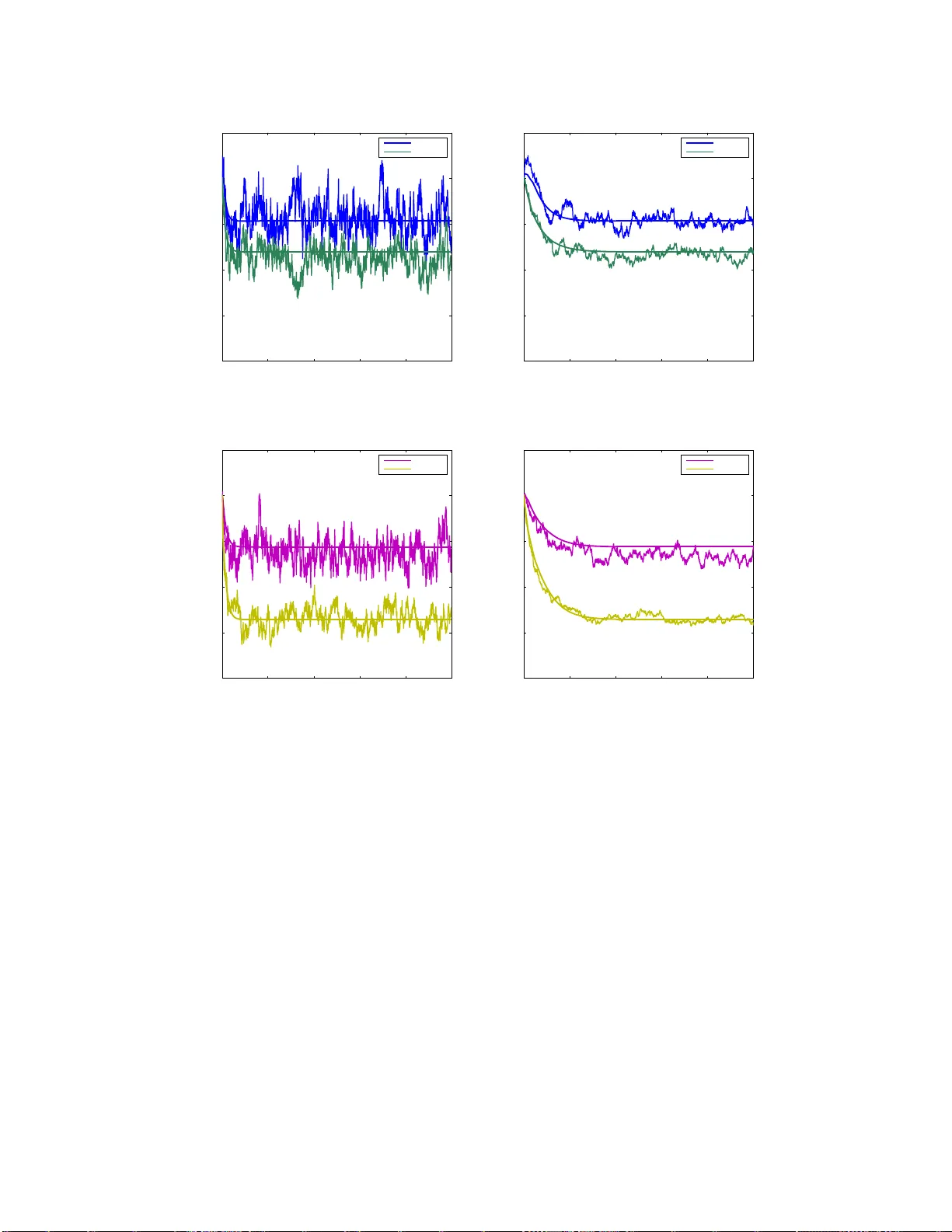
1 Optimizing Orthogonal Multiple Acc ess based on Quantized Channel Sta te Information Antonio G. Marques, Georg ios B. Giannakis, and Ja vier Ramos Abstract The perf ormance of systems where multip le users co mmunicate over wireless fading links beneﬁts fro m channel- adaptive allocation of the a vailable resources. Different from most existing app roaches that allocate re- sources based on perfect channel state info rmation, this work optim izes c hannel scheduling a long with p er user rate and power loadings over orthogo nal fading chann els, when both terminals and sched uler rely o n qu antized chann el state inform ation. Chan nel-adap ti ve p olicies are designed to optim ize an average tran smit-perfo rmance criterion subject to average qu ality of ser vice req uiremen ts. While the resultant optimal po licy pe r fading r ealization shows that the individual rate and power loadin gs can be ob tained separ ately f or each user , the optim al sched uling is slightly more co mplicated. Speciﬁcally , p er fading realization each chann el is allocated either to a single (winner) user , o r , to a small gro up of winner users whose percentage of sh ared resources is f ound by solving a linear progr am. A single sch eduling scheme co mbining both alternatives becomes po ssible by smo othing the or iginal disjoint scheme. The smo oth scheduling is asympto tically optim al and in curs r educed computationa l complexity . Different alternati ves to obtain the Lagr ange multipliers required to implement the channel- adaptive policies are propo sed, includin g stochastic iterations that are provably con vergent and do not requir e kn owledge o f the ch annel distribution. The d ev elopmen t of the o ptimal ch annel-ad aptive allocation is compleme nted with discussions on the overhead requir ed to implemen t th e n ovel policies. I . I N T R O D U C T I O N The importance of channel-adaptive allocation of bandwidth, rate, and power resources in wireless multiuser access o ver fading lin ks has been well documented from both informati on theoretic and practical communication perspecti ves [2]. Per f ading realization, parameters i ncluding rate, power and percentages of time f rames (or system subcarriers) ar e adjusted a cross users to optimize utility measures of performance quantiﬁed by bit error rate (BER), weighted sum-rate or p ower ef ﬁciency , under quality of service (QoS) constraints such as prescribed BER, delay , maximum power or minimum rate requirements. T o carry out such constrained op timization t asks, m ost existing approaches ass ume that perfect CSI (P-CSI) is av ai lable where ver needed [17], [6], [9], [1 0], [19], [21]. Howe ver , it is well appreciated that errors in estimating the channel, feedback delay , and th e asymmet ry between forward and reverse links render acquisition of W ork in this paper w as supported by t he NSF grants CCF 0830480 and CON 08240 07; USDoD AR O Grant No. W911NF-05-1-0283 ; C.A. Madrid Grant No. P-TIC- 000223 -0505; S panish Govern ment Grant No. TEC2009-12098; and also through collaborative participation in the Communications and Networks Consortium sponso red by the U. S. Army Research L aboratory under the Collaborati ve T echnology Alliance Program, Cooperativ e Agreement DAAD19-01 -2-0011. The U.S . Governmen t is authorized to reproduce and distri bute reprints for Gov ernment purposes notwithstanding any copyrigh t notation thereon. Part of this paper was presented in the IEEE Intl. W orkshop on Signal Pr ocess. Advances in W ireless Commun. , Recife, Brasil, July 2008. A. G. Marques and J. Ramos are with the Department of Signal Theory and Commun i cations, Rey Juan Carlos Univ ersit y , Camino del Molino s/ n, F uenlabrada, Madrid 289 43, Spain, e-mails: antonio.garcia.marques@urjc.es, javier .ramos@urjc.es G. B. Giannakis is with t he Department of Electrical and Computer Engineering, Univ ersit y of Minnesota, 200 Union S treet SE, Minneapolis, MN 554 55, USA, e-mail: georgios@umn.edu 2 deterministicall y perfect CSI at transmitters (P-CS IT) imp ossible in m ost wireless scenarios [8]. F or cases where the schedul ing takes place at the recei ver , this has motiv ated scheduling and resource allocation schemes using perfect CSI at the recei vers (P-CSIR) but only quantized CSI at the transmit ters (Q-CSIT), that can be pragmatically obtained through ﬁnite-rate feedback from the recei ver , see, e.g., [13], [18 ], and also [11] for a recent re vi e w on ﬁnite-rate feedback sy stems. This work goes one step further to pursue optim al schedul ing and resource allocation for orth ogonal multi-access t ransmission s ov er fading l inks when o nly Q-CSI is av ailable at the scheduler (as, e.g. , [5] for the non-orthog onal m ultiple input multiple output -MIMO - case), while transmit ters have eit her perfect or q uantized CSI. The unifying approach minimizes an a verage power cost (or in a dual formulati on maximizes an av erage rate uti lity) subj ect to a verage Qo S cons traints on rate (respecti vely power ) related constraints. This setup is p articularly suited for syst ems where the recei ver does not ha ve accurate channel estimates (e.g., wh en diffe rential (de-)modulati on is emp loyed or when the fading channel varies fast). It is als o pertinent in distributed set-ups (sensor networks or cellular downlink comm unications), wh ere the scheduler (fusion center , access po int) is not the receiv er and can only acquire Q-CSI sent by the terminals. The disti nct features of this paper are: • O ptimal resource allocati on schemes that adapt rate, po wer , and user scheduling as a fun ction of the instantaneous Q-CSI. • T he optimal rate and power loadings per user terminal depend on the Q-CSI corresponding to its own fading realization, it s relative contribution to the power cost (qu antiﬁed through a user-dependent priority weight ), and its rate requirement. • T he optimal scheduling per channel b oils down to one out of two modes: (i) a single u ser accessing the channel; or , (ii ) a small set of us ers sharing the channel. The channel access coefﬁcients under (ii) are o btained as the solution of a linear program. This bim odal pol icy emerges not only in system s that operate based on Q-CSI, but also in thos e that rely on P-CSI but operate over channels whose probability densi ty function (pdf) contains deltas (e.g., discrete random channels or deterministi c channels). • A novel asymptotically optimum scheduling scheme facilitating con ver gence and reducing complexity . This scheme combines the aforementioned cases (i) and (ii), and only incurs an ε -l oss relative t o th e optimal so lution (wit h ε representing a s mall positive number). • Sto chastic allocation schemes that are prov ably con vergent, without requiring knowledge of t he channel dis tribution, while reducing the complexity of the ov erall design. • O perating condi tions under which the system overhead can be reduced are identiﬁed. In additio n, t he approach here uniﬁes no tation at the receiving and transmitti ng ends, and clariﬁes the model w hen Q-CSI i s av ailable, yi elding valuable insight s for imp rove d understanding o f channel-adaptive resource all ocation and ﬁnite-rate feedback. The rest of the paper is organized as follows. After modeling preli minaries in Section II, the general problem is formu lated in Section II-A, and the optimal solut ion is characterized in Sec tion III. Algorithms to obtain the optim um L agrange multip liers needed to im plement the optimal policies are dev eloped i n Section IV. Those algorit hms rely on a novel sm ooth scheduling policy th at reduces complexity and guarantees asym ptotic opti mality . Stochastic scheduling al gorithms that do not require k nowledge of the channel distribution are als o d e veloped. Section V provides examples and ins ights on the practical 3 implementati on of the novel channel-adaptiv e schemes. Numerical tests corroborating t he analytical claim s are described in Section VI, and conclud ing remarks are off ered i n Section VII. 1 I I . P R E L I M I N A R I E S A N D P R O B L E M S TA T E M E N T Consider a wireless network with M user terminals, indexe d b y m ∈ { 1 , . . . , M } , transmitti ng over K ﬂat-fading ortho gonal channels, indexed by k ∈ { 1 , . . . , K } , to a commo n desti nation, e.g., a fus ion center or an access poin t. Zero-mean additive white Gaussi an noise (A WGN) with unit variance is assumed present at the recei ver . W ith g m,k denoting the k th channel’ s instantaneous gain (magnitude sq uare of t he fading coef ﬁcient) between t he m th user and the destination, the overa ll channel is described by the M × K gain matrix G for which [ G ] m,k := g m,k . The range o f values each g m,k takes is divided int o non- overlapping regions; and inst ead of g m,k itself, destination and transmitters have av ailable on ly t he binary code word indexing the region g m,k falls into. W ith j m,k representing the correspondi ng region index, the M × K matrix J with entries [ J ] m,k := j m,k constitutes the Q-CSI of the overall syst em. Since g m,k is random, j m,k is also a discrete random v ariable; and likewise J is random, taking matrix values from a set J w ith ﬁnit e cardinal ity | J | . As i n [21 ], [13], [9] or [19], users at the outset can be scheduled to access sim ultaneously but orthogonally (in time or frequency) any of the K channels. The channel scheduli ng po licy is described by an M × K matrix W w hose nonnegati ve entry [ W ] m,k corresponds to the per centage of th e k th channel scheduled for the m th user . Clearly , it holds that P M m =1 [ W ] m,k ∈ [0 , 1] ∀ k . The power and rate resources of all terminal-channel pairs are collected in M × K matri ces P and R , respectively . Each of the correspondin g entries [ P ] m,k and [ R ] m,k represent, respectively , t he nominal power and rate th e m th user t erminal would be allocated if it were the on ly terminal scheduled to transmi t over the k th channel. Note that su ch entries are lower bo unded by zero and upper bo unded by the maximu m nom inal power and rate that t he hardware of the system is able to i mplement. Since scheduling and allo cation will be adapted based on Q-CSI, matrices W , P and R wil l depend on J and each can take at most |J | diffe rent v alues. Under prescribed BER or capacity constraints, rate and po wer variables are coup led. T his power -rate coupling wi ll be represented by a functi on Υ (respectively Υ − 1 for the rate-po wer coup ling), which relates [ P ] m,k to [ R ] m,k over the s ame Q-CSI region R ([ J ] m,k ) . (Wherev er needed, w e will write Υ R ([ J ] m,k ) to exemplify this dependence.) A. P r oblem F ormulation Giv en the Q-CSI matrix J and prescribed QoS requirements, the goal is to ﬁnd W ( J ) , P ( J ) and R ( J ) so that the overall a verage weighted performance is optimized. (Overall here refers to performance of all users and weighted refers to different user priorities ef fected th rough a preselected weight vector µ := [ µ 1 , . . . , µ M ] T with nonnegativ e ent ries.) Depending on desirable objectives, the problem can be formulated either as constrained u tility maxim ization of the a verage weighted sum-rate subject to a verage 1 N otation: Boldf ace upper (lower) case letters are used for matrix (column vectors); ( · ) T denotes transpose; [ · ] k,l the ( k , l ) th entry of a matrix, and [ · ] k the ( k ) th column (entry) of a matrix (vector); ⊙ stands for entrywise (Hadamard) matrix product; · denotes differe ntiation; 1 and 0 are the all-one and all-zero matrices. Calligraphic letters are used for sets with |X | denoting cardinality of the set X . For a random scalar (matrix) v ariable x ( X ), the univ ariate (multi variate) probability density function (pdf) is denoted by f x ( x ) (respectiv el y f X ( X ) ). Finally , ∧ ( ∨ ) deno tes the “and” (“or”) l ogic operator , x ∗ the optimal v alue of v ariable x ; and , 1 {·} the indicator function ( 1 { x } = 1 if x is true and zero otherwise). 4 power constraints; o r , as a cons trained m inimizatio n of the av erage weig hted po wer subj ect to ave rage rate constraints . The former ﬁts the classical rate (capacity) maximi zation, while th e latter is particularly rele vant in energy-limited scenarios (e.g., sensor networks) where power savings is the m ain objectiv e. Although this p aper wi ll use the power minimization formulation, the rate maxim ization problem can be tackled readily b y dual s ubstituti ons; namely , after int erchanging the roles of R and Υ R ([ J ] m,k ) by P and Υ − 1 R ([ J ] m,k ) , respecti vely . Speciﬁcally , the weighted average transmit-power will be mi nimized subject to individual minimum a verage rate const raints collected in the vector ˇ r := [ ˇ r 1 , . . . , ˇ r M ] T . Per Q-CSI realization J , t he overall weighted transm it-power is given by P M m =1 [ µ ] m P K k =1 [ P ( J )] m,k [ W ( J )] m,k ; while the m th user’ s transmit- rate is P K k =1 [ R ( J )] m,k [ W ( J )] m,k . Using the probabil ity mass function Pr { J } , these expressions can be used t o obtain t he aver age transmi t-power and transmit-rate. For a g iv en channel quantizer , i.e., with R ﬁxed, and the fading pdf assumed known, Pr { J } can be obtained as Pr { J } = R R ( J ) f G ( G ) d G , where R ( J ) represents t he region of the G do main su ch that G ∈ R ( J ) are q uantized as J . Since Υ R ([ J ] m,k ) links R wi th P , it sufﬁces to opti mize only over one of them. Note also that the binomial [ R ( J )] m,k [ W ( J )] m,k is not jointly con vex wit h respect to (w .r .t.) R ( J ) and W ( J ) . F or t his reason, we will instead consider the auxiliary variable [ ˜ R ( J )] m,k := [ R ( J )] m,k [ W ( J )] m,k and seek allocation and scheduling matrices s olving the following opt imization prob lem:              min ˜ R ( J ) ≥ 0 , W ( J ) ≥ 0 X ∀ J ∈J  P M m =1 [ µ ] m P K k =1 Υ R ([ J ] m,k )  [ ˜ R ( J )] m,k [ W ( J )] m,k  [ W ( J )] m,k  Pr { J } s . to : X ∀ J ∈J  P K k =1 [ ˜ R ( J )] m,k  Pr { J } ≥ [ ˇ r ] m , ∀ m P M m =1 [ W ( J )] m,k ≤ 1 , ∀ k , ∀ J . (1) Appendix A sh ows that if Υ R ([ J ] m,k ) is a con vex function, then problem (1) i s con vex. Throughout this paper i t wil l be assumed that: (as1) the power-rate function Υ R ([ J ] m,k ) is incr easing and s trictly con vex . This assumpti on ho lds generally true for orthogon al access but, for example, n ot when m ultiuser inter- ference is p resent. Note al so that (as1) im plies that the rate-power functio n Υ − 1 is i ncreasing and s trictly conca ve. T o justify t he adopti on of (as1), consider t he following exa mple of Υ . Example 1 : For simplicity , the tractable c ase of outage ca pacity will be consider here, postponin g the case of ergodic capacity to Section V -D. Suppose that we want the outage probability of the m th user over the k th channel for a given Q-CSI J to be δ . Deﬁne the δ -outage channel gain for the ( m, k ) pair in R ([ J ] m,k ) as g δ m,k ([ J ] m,k ) so that Pr { g m,k ≤ g δ m,k ([ J ] m,k ) | g m,k ∈ R ([ J ] m,k ) } = δ . Then using Shannon’ s capacity formula, the rate-power function can be written as Υ − 1 R ([ J ] m,k ) ( x ) = log 2 (1 + xg δ m,k ([ J ] m,k )) . Solving the pre vious expression w .r .t. x , yield s the power -rate function Υ R ([ J ] m,k ) ( x ) = (2 x − 1) /g δ m,k ([ J ] m,k ) , which is certainly in creasing and strictly con ve x as required by (as1). Before m oving to the next section where the solutio n of (1) will be characterized, it is i mportant to stress that since R i s in volved in specifying Pr { J } and Υ R ([ J ] m,k ) , the choice of R af fects th e optimum allocation. Selecting the quantization regions to opti mize (1) is t hus of interest b ut goes beyond the scope of this paper . Near-optimal channel quantizers for tim e division mul tiple access (TDMA) and orthogonal frequency-di vis ion multiple access (OFDMA) can be found in [18] and [13], respectively . 5 I I I . O P T I M U M R E S O U R C E A L L O C A T I O N In this section, the op timum W , P and R matrices will be characterized as a function of J and the optimum multipliers of the constrained optimization prob lem in (1). Let λ R denote the M × 1 ve ctor whose entries are the non-negativ e Lagrange mult ipliers associated with the m th avera ge rate const raint; and λ W ( J ) the K × 1 vector correspon ding to the k th channel-sharing constraint per Q-CSI matrix 2 J . Let also α R ( J ) and α W ( J ) denote K × M matrices whose entries are, correspondingly , the non-negative L agrange mult ipliers associated with the cons traints [ ˜ R ( J )] m,k ≥ 0 and [ W ( J )] m,k ≥ 0 . The full Lagrangian of (1) can b e wri tten as L ( λ R , λ W ( J ) , α R ( J ) , α W ( J ) , ˜ R ( J ) , W ( J )) := X ∀ J ∈J M X m =1 [ µ ] m K X k =1 Υ R ([ J ] m,k ) [ ˜ R ( J )] m,k [ W ( J )] m,k ! [ W ( J )] m,k ! Pr { J } − M X m =1 [ λ R ] m X ∀ J ∈J K X k =1 [ ˜ R ( J )] m,k ! Pr { J } − [ ˇ r ] m ! + X ∀ J ∈J K X k =1 [ λ W ( J )] k M X m =1 [ W ( J )] m,k − 1 ! − X ∀ J ∈J M X m =1 K X k =1  [ α R ( J )] m,k [ ˜ R ( J )] m,k + [ α W ( J )] m,k [ W ( J )] m,k  . (2) Because (1) is con vex, th e Karush-Kuhn-T ucker (KKT) conditions y ield the foll owing necessary and sufﬁ cient condi tions of optim ality [1] (recall ˙ x deno tes the deriv ative of x ): [ µ ] m ˙ Υ R ([ J ] m,k ) [ ˜ R ∗ ( J )] m,k [ W ∗ ( J )] m,k ! Pr { J } − [ λ R ∗ ( J )] m Pr { J } − [ α R ∗ ( J )] m,k = 0 (3) [ ˜ R ∗ ( J )] m,k [ α R ∗ ( J )] m,k = 0 (4) [ µ ] m Υ R ([ J ] m,k ) [ ˜ R ∗ ( J )] m,k [ W ∗ ( J )] m,k ! Pr { J } − [ µ ] m ˙ Υ R ([ J ] m,k ) [ ˜ R ∗ ( J )] m,k [ W ∗ ( J )] m,k ! [ ˜ R ∗ ( J )] m,k [ W ∗ ( J )] m,k Pr { J } − [ α W ∗ ( J )] m,k + [ λ W ∗ ( J )] k = 0 (5) [ W ∗ ( J )] m,k [ α W ∗ ( J )] m,k = 0 . (6) Conditions (3)-(6 ) can be used to characterize th e optim al rate and channel allocati on as follows. Pr oposition 1: The opti mum rate allocat ion is given by: (i) [ ˜ R ∗ ( J )] m,k = 0 , if either [ W ∗ ( J )] m,k = 0 or [ λ R ∗ ] m / [ µ ] m < ˙ Υ R ([ J ] m,k )  [ ˜ R ∗ ( J )] m,k [ W ∗ ( J )] m,k  ; o therwise, (ii) the opti mum rate allocation is [ ˜ R ∗ ( J )] m,k = ˙ Υ − 1 R ([ J ] m,k )  [ λ R ∗ ] m [ µ ] m  [ W ∗ ( J )] m,k (7) wher e ˙ Υ − 1 R ([ J ] m,k ) denotes the inv erse functi on of ˙ Υ R ([ J ] m,k ) . Pr oof: Consider ﬁrst the claim in (i). The deﬁnition of [ ˜ R ∗ ( J )] m,k implies that if [ W ∗ ( J )] m,k = 0 , then [ ˜ R ∗ ( J )] m,k = 0 . On the ot her hand, if [ λ R ∗ ] m / [ µ ] m < ˙ Υ R ([ J ] m,k ) ( · ) , then (3) can only be satisﬁed if [ α R ∗ ( J )] m,k > 0 . Using the slackness cond ition i n (4), the latter implies [ ˜ R ∗ ( J )] m,k = 0 . The proof of part (ii) i s si mpler and consists of solving (3) after excluding the two cases in (i); i.e. assuming that 2 The dependence of the multipliers associated with instantaneous constraints on J will be explicitly wr itten t hroughou t . 6 [ W ∗ ( J )] m,k > 0 and [ α R ∗ ( J )] m,k = 0 . Given the relationship betwee n ˜ R and R , the optimum transmit -rate for [ W ∗ ( J )] m,k 6 = 0 is [ R ∗ ( J )] m,k = ˙ Υ − 1 R ([ J ] m,k )  [ λ R ∗ ] m [ µ ] m  . (8) In fact, (8) is also valid if [ W ∗ ( J )] m,k = 0 . This is because when [ W ∗ ( J )] m,k = 0 , any ﬁnite nominal rate yields [ R ∗ ( J )] m,k = 0 , which is the opt imal so lution. Equation (8) shows that th e opt imal rate lo ading depends on the ratio of [ µ ] m over [ λ R ∗ ] m , where the ﬁrst represents th e “priorit y” terminal m has t o minimize the total power cost, and the l atter represents t he price correspondi ng its rate requirement . According to (as1), ˙ Υ is mon otonically increasing function and so is ˙ Υ − 1 in (8). This implies that users with high [ ˇ r ] m hav e hi gh values of [ λ R ∗ ] m , thu s higher rate and power loadings per region. Con versely , for users whose powe r consumption is critical the opt imum so lution s ets high v alu es of [ µ ] m , thus lo w rate and power loadings per region. Part (i ) of th e proposit ion also dictates that there may be regions for which the optimum rate and power loadings are zero. Intuitively , this wil l t ypically happen for the region(s) whose channel condi tions are so poor that the power cos t of activ ating the region may be too high. T o ﬁnd the optimum schedul ing m atrix W , deﬁne ﬁrst the functional [ C W ( J )] m,k := [ µ ] m Υ R ([ J ] m,k ) ([ R ∗ ( J )] m,k ) − [ λ R ∗ ] m [ R ∗ ( J )] m,k (9) which represents the cost of scheduling channel k to us er m when the Q-CSI is J . This cost of selecting [ W ( J )] m,k = 1 emerges also in the two ﬁrst terms o f L in (2). Based on (9), and with ∧ denoting the “and” operator , we deﬁne t he K × 1 vector c ∗ W ( J , λ R ) with entries [ c ∗ W ( J , λ R )] k := min m { [ C W ( J , λ R )] m,k } M m =1 , and the sets of “winner user(s)” M ( J , k ) := { m : [ C W ( J , λ R )] m,k = [ c ∗ W ( J , λ R )] k ∧ ([ c ∗ W ( J , λ R )] k < 0 ) } . Giv en th e Q-CSI realizatio n J , M ( J , k ) is the set of user(s) that in cur the mi nimum cost if scheduled to access channel k wh ile [ c ∗ W ( J , λ R )] k is the cost correspond ing to those users. Usin g these notational con ventions, it can be shown th at: Pr oposition 2: The opti mum scheduling W ∗ ( J ) satisﬁes the foll owing: (i) If [ W ∗ ( J )] m,k > 0 , then m ∈ M ( J , k ) ; (ii) If |M ( J , k ) | > 0 , then P m ∈M ( J ,k ) [ W ∗ ( J )] m,k = 1 ; and (iii) If |M ( J , k ) | = 0 , then [ W ∗ ( J )] m,k = 0 ∀ m . Pr oof: Appendix B. In words, the optimal scheduler assigns t he channel only to user(s) with minim um negative cost (9), which i s in most cases (but not all) att ained by a single user . This is a greedy policy because o nly one user with mi nimum cos t is selected to transmit per Q-CSI realization, while o thers defer . Note that with P-CSIR, the opt imum scheduling over orthogonal fading channels is also greedy , whether based on P-CSIT [9], [19] or Q-CSIT [13]. Case 1 (Single winner us er): When the minim um cost i s attained by only on e user , W ∗ in Proposition 2 can b e writ ten usi ng th e i ndicator functi on, as [ W ∗ ( J )] m,k = 1 { m ∈M ( J ,k ) } . (10) Since [ C W ( J )] m,k is a function o f dif ferent variables (nam ely , the quantization regions, the fading real- ization, the i ndividual priority weight and the individual Lagrange m ultiplier), for most CSI realizations the costs correspondi ng to different users m are dist inct, and the em er g ing winner is unique. 7 Case 2 (Mult iple winners): The e vent of having di f ferent users attain ing the mi nimum cost will be henceforth referred to as a “tie”. The m ain difﬁculty with a ti e is that Proposition 2- (ii) d oes not specify how the channel sho uld be split among winner users (th e underlying reason being that any arbitrary allocation minimizes L ). On the other hand, only a subset (for m ost realizations one) of them is the actual solution to t he original primal prob lem. T o ﬁnd the optimu m schedule in this case, deﬁne ﬁrst the m atrix of single-winner scheduling as [ W one ( J )] m,k := [ W ∗ ( J )] m,k in (10) for all ( J , k ) so that |M ( J , k ) | = 1 , and [ W one ( J )] m,k := 0 , otherwise. Deﬁne further the schedul ing m atrix with mult iple winners as [ W tie ( J )] m,k = 0 if |M ( J , k ) | ≤ 1 or if |M ( J , k ) | > 1 but m / ∈ M ( J , k ) , and [ W tie ( J )] m,k ∈ [0 , 1] , otherwise. And ﬁnally , let th e set of mult iple-winner scheduling m atrices be W tie := { W tie ( J ) | ∀ J } ; t he a verage single-winner transm it-rate vector [ ¯ r one ] m := P ∀ J  P K k =1 [ R ∗ ( J )] m,k [ W one ( J )] m,k  Pr { J } ; and ˇ r tie := ˇ r − ¯ r one . Using t hese deﬁnitions, the optimum schedule W tie ( J ) for all ( J , k ) with |M ( J , k ) | > 1 , can b e foun d as the solutio n of the following linear program:            min W tie ( J ) ∈W tie P ∀ J  P K k =1 P M m =1 [ µ ] m Υ R ([ J ] m,k ) ([ R ∗ ( J )] m,k ) [ W tie ( J )] m,k  Pr { J } s . to : P ∀ J  P K k =1 [ R ∗ ( J )] m,k [ W tie ( J )] m,k  Pr { J } = [ ˇ r tie ] m , ∀ m P M m =1 [ W tie ( J )] m,k = 1 , ∀ ( J , k ) : |M ( J , k ) | > 1 . (11) Note that in the optimi zation process, only th e m atrices J for which a tie occurs are consi dered and for those o nly th e n on-zero ent ries of W tie ( J ) are opt imized. The main idea behind (11) is that am ong all schedules m inimizin g the Lagrangian when a tie occurs (second constraint), the optimal one for the primal problem is the one for which the a verage rate constraints are satisﬁed with equality . W e stress that here R ∗ ( J ) (thus P ∗ ( J ) ) are ﬁxed and therefore only optimi zation over the channel-sharing coef ﬁcients for whi ch a tie occurs (which in general is a small set) is carried out. T o clarify this po int, let us consider the following e xample. Example 2 : Consi der a system with K = 1 channel, M = 4 users and 10 regions per user . For such a system, the number of channel realizations is |J | = 10 4 . Among those i t is found that, e.g., ti es occur for 3 different fading realizations, n amely: when J = J 1 users 1 and 2 tie; when J = J 2 users 1, 3 and 4 t ie; and when J = J 3 users 2 and 4 tie. In th is case, th e opt imization in (11) has to be carried out ov er [ W ( J 1 )] 1 , 1 , [ W ( J 1 )] 2 , 1 , [ W ( J 2 )] 1 , 1 , [ W ( J 2 )] 3 , 1 , [ W ( J 2 )] 4 , 1 , [ W ( J 3 )] 2 , 1 , and [ W ( J 3 )] 4 , 1 . Once W ∗ tie ( J ) is found, the overall optimal channel assi gnment is [ W ( J ) ∗ ] m,k := [ W ∗ one ( J )] m,k for ( J , k ) with |M ( J , k ) | ≤ 1 and [ W ∗ ( J )] m,k := [ W ∗ tie ( J )] m,k otherwise. It is worth noticing that for every scenario where m ultiple us ers access the channel orthogo nally , the optimum scheduling needs to satisfy (11). Howe ver , neither [9], [19] (P-CSIR and P-CSIT) no r [13], [18] (P-CSIR and Q-CSIT) consider (11). This is b ecause if the fading dis tributions are conti nuous and P-CSIR is a va ilable, the set o f fa ding realizations G for which a tie occurs has Lebesgue measure zero. Therefore, any arbitrary channel scheduling among ti ed users is equally optimum. Indeed, the contribution of any speciﬁc G to the ave rage p erformance when integrated over the channel pdf i s zero. But when dealing with Q-CSI (or with deterministic ﬁxed channels), neither the p robability of a Q-CSI realization J nor the contribution to th e average cost are negligible. And this precisely necessitates sol ving (11 ) to obtain the optimum schedule. Intu itive ly , as t he n umber of regions and chann els increases sharing a channel becomes less likely , which in turn brings the solution closer to the continuous fading P-CSIR case and the ef fect of neglecting (11) becomes less harmful . The opposi te beha vi or arises in sy stems that have P-CSIR 8 but furt her operate over deterministi c (ﬁxed) channels. In th ose systems ties wi ll represent t he prev aili ng channel all ocation (e.g., for a determinis tic TDMA system we hav e K = 1 and |J | = 1 ; s ince all the users have t o access th e channel t o satisfy their rate con straints, the entries of λ R ∗ will self-adjust s o that a tie among a ll the users occurs). Only in systems operatin g over determi nistic channels for which the number of channels is much high er than the number of users (e.g., an OFDMA system with m any subcarriers), t he single-winner case will constitute t he predomi nant schedul ing. In the context of smooth optim ization, a si ngle s cheduling scheme that can b e implement ed both for cases 1 and 2, i s asymptotically optimal, incurs reduced computational b urden and facilitates com putation of the optim al Lagrange multi pliers is de veloped in the next s ection. I V . O P T I M A L L AG R A N G E M U LT I P L I E R S T o implement t he opt imum scheduling and rate allocation policies presented in the previous section, the opt imum m ultiplier vector λ R ∗ needs to be known. Since the rate constraint s in (1) are always active , the KKT condi tions im ply that when λ R = λ R ∗ those constraints are satisﬁed with equality . Since λ R ∗ cannot be obtained analytically from this cond ition, numerical search is requi red. This is possib le using dual m ethods. First, let us write 3 a s impliﬁed version of th e Lagrangi an L ( λ R , ˜ R ( J ) , W ( J )) := X ∀ J ∈J M X m =1 [ µ ] m K X k =1 Υ R ([ J ] m,k ) [ ˜ R ( J )] m,k [ W ( J )] m,k ! [ W ( J )] m,k ! Pr { J } − M X m =1 [ λ R ] m X ∀ J ∈J K X k =1 [ ˜ R ( J )] m,k ! Pr { J } ! + M X m =1 [ λ R ] m [ ˇ r ] m (12) where only t he contribution o f the av erage rate constraints is considered [cf. (2)]. Because all th e instantaneous const raints (i.e., channel-sharing and non-negativity c onstraints) were already satisﬁed when obtaining the sol ution of the previous section, the focus here is to ﬁnd λ R so that th e av erage rate constraints are satis ﬁed. Let F ( J ) denot e the feasible set of t he rate and channel assignment matrices, namely F ( J ) := { ( ˜ R ( J ) , W ( J )) | ˜ R ( J ) ≥ 0 ∧ W ( J ) ≥ 0 ∧ P M m =1 [ W ( J )] m,k ≤ 1 } . The dual function is th en deﬁned as D ( λ R ) := inf ( ˜ R ( J ) , W ( J )) ∈F ( J ) L ( λ R , ˜ R ( J ) , W ( J ) ) = L ( λ R , R ∗ ( J , λ R ) ⊙ W ∗ ( J , λ R ) , W ∗ ( J , λ R )) (13) which is concave w .r .t. λ R . Based on (13), the dual p roblem of (1) is max λ R ≥ 0 D ( λ R ) . (14) Since the problem in (1) is con vex and strictly feasible, the duali ty gap between the pri mal and dual problems is zero. Thus, the value of λ R optimizing (14) can be used t o ﬁnd the optimum primal solut ion. A standard approach to obtain λ R ∗ is to implement a subgradient iteration (a gradient itera tion is impo ssible here because D ( λ R ) is non-di f ferentiable w .r .t. [ λ R ] m ). Let ∂ D ( λ R ) denote a subgradient vector o f (13 ) whose m th entry is [ ∂ D ( λ R )] m := [ ˇ r ] m − P ∀ J P ∀ k [ R ∗ ( J , λ R )] m,k [ W ∗ ( J , λ R )] m,k Pr { J } ; let a lso i d enote 3 Throughout this secti on, dependence on λ R will be made e xplicit wherev er it contributes to clari ty . 9 an iteration index, and β ( i ) a decreasing small s tepsize such that P ∞ i =1 β ( i ) = ∞ and P ∞ i =1  β ( i )  2 < ∞ . W ith these choices, the iterations λ R ( i ) = λ R ( i − 1) + β ( i ) ∂ D ( λ R ( i − 1) ) (15) con ver ge to λ R ∗ as i → ∞ (cf. [1, Sec. 6.3.1]). A m ajor challenge in o btaining λ R ∗ using (15) is th at [ ∂ D ( λ R )] m is discont inuous because W ∗ ( J , λ R ) is not cont inuous for ev ery λ R that gives ris e to a tie. This problem i s critical, b ecause in m ost cases λ R ∗ is one of th e points where [ ∂ D ( λ R )] m is di scontinuous. Note that discon tinuity of the prim al solutio n at λ R ∗ implies that obt aining a solution arbitrarily cl ose to the opt imal in the dual domain, does not guarantee obtain ing a solution arbitrarily close to the optim al in the primal dom ain. Speciﬁcally , after running a suf ﬁciently hi gh but ﬁnit e n umber of iterations I , we can guarantee that λ R ( I ) is a very good approximation for λ R ∗ , but we cannot guarantee that W ∗ ( J , λ R ( I ) ) is a good approximation of W ∗ ( J , λ R ∗ ) . In fact, it can be shown that such schedu lings are signiﬁcantly diffe rent for a sub set of channel realizations J , and that the schedul ing W ∗ ( J , λ R ( I ) ) is not a feasibl e solution of (1) since it violates t he ave rage rate constraints . Our approach to solve this problem is to reinstate Lipschitz continuity by smoothing the schedul ing function. Smoothing ensures continu ity or dif ferentiabi lity and has been su ccessfully appl ied to differe nt optimizatio n probl ems; see e.g., [22] and [14]. Since scheduling discont inuities app ear in the transition from a tie to a single-winner (check (10), (11) and t he left and right upper plot s of Figure 1), the id ea is to relax the condit ion for schedul ing in the k th channel only when m ∈ M ( J , k ) . This is possible through the set M s ( J , k ) := { m : ([ C W ( J , λ R )] m,k − [ c ∗ W ( J , λ R )] k < ε ) ∧ ([ c ∗ W ( J , λ R )] k < 0) } , wh ere ε is a small p ositive num ber . Based on M s ( J , k ) , consi der the following subop timal but smooth s cheduling matrix [ W s ( J , λ R )] m,k := 1 { m ∈M s ( J ,k ) }  1 − [ C W ( J , λ R )] m,k − [ c ∗ W ( J , λ R )] k ε  2 P m ∈M s ( J ,k )  1 − [ C W ( J , λ R )] m,k − [ c ∗ W ( J , λ R )] k ε  2 . (16) Clearly , [ W s ( J , λ R )] m,k schedules channel k no t only t o u sers m whose cost is m inimum but also to t hose whose cost is ε -close to the mini mum. Thi s can be readily app reciated in the left lower and right lower plots of th e example illust rated in Figure 1. A ccording to the upper left plot, when [ λ R ] 2 ∈ (3 . 45 , 3 . 5) the opt imum allo cation assi gns the channel t o user 1, meaning that it s cost is the lowest in that in terva l. Howe ver , according t o the lo wer righ t plot, when [ λ R ] 2 ∈ (3 . 4 5 , 3 . 5 ) the smooth all ocation assigns a portion of t he channel also t o user 2. This is because although the cost of user 1 is stil l smaller , within that interval the d iffe rence of costs between the two users i s less th an ε . Something simil ar happens when [ λ R ] 2 ∈ (3 . 5 , 3 . 55 ) , but in this case user 2 is the o ne with the smallest cost . The scheduli ng in (16) exhibits other rele vant properties that are summ arized in th e next Proposition . Pr oposition 3: The smoot h scheduler W s ( J , λ R ) satisﬁes the follo wing: (i) If [ W s ( J , λ R )] m,k > 0 , then m ∈ M s ( J , k ) and [ C W ( J , λ R )] m,k < [ c ∗ W ( J , λ R )] k + ε ; (ii) If |M s ( J , k ) | > 0 , P m ∈M s ( J ,k ) [ W s ( J , λ R )] m,k = 1 ; (iii) If |M ( J , k ) | = 0 , then [ W s ( J , λ R )] m,k = 0 ∀ m ; and (iv) [ W s ( J , λ R )] m,k is a conti nuous functi on of λ R . Pr oof: The construction of t he scheduli ng matrix (16) can be readily used to verify the claims (i)-(iv). Properties (i)-(iii) of W s are si milar to those of W ∗ stated in Proposition 2, while (i v) ensu res contin uity 10 3 3.5 4 0 0.5 1 [ λ R ] 2 [ W ∗ ( J , λ R )] 1 , k (3 . 5 , 0 . 2 5 ) 3 3.5 4 0 0.5 1 [ λ R ] 2 [ W ∗ ( J , λ R )] 2 , k (3 . 5 , 0 . 7 5 ) 3 3.5 4 0 0.5 1 [ λ R ] 2 [ W s ( J , λ R )] 1 , k (3 . 5 2 , 0 . 2 5 ) 3 3.5 4 0 0.5 1 [ λ R ] 2 [ W s ( J , λ R )] 2 , k (3 . 5 2 , 0 . 7 5 ) Fig. 1. Optimal (top) and smooth (bottom) channel allocation for t he k th channel as [ λ R ] 2 v ari es. The simulated set-up is: M = 2 , ε = 0 . 01 , [ λ R ] 1 = λ 0 is kept constant, and [ C W ( J , λ R )] 1 ,k = [ C W ( J , λ R )] 2 ,k when [ λ R ] 1 = λ 0 and [ λ R ] 2 = 3 . 5 . (check l ower plots in Figure 1). Besides being continuous, the smoot h scheduling also lowers complexity relativ e to its discontin uous counterpart. In fact, wh en a tie occurs, ﬁndin g W ∗ ( J ) requires solv ing a lin ear program t hat in volves channel realizations other than J (recall Example 2 ), whil e ﬁnding W s ( J ) requires only the computation of the closed form in (16) without having to consider any channel realization other than J . Based on Proposition 3, t he following result can be established. Lemma 1 : If D s ( λ R ) := L ( λ R , R ∗ ( J , λ R ) ⊙ W s ( J , λ R ) , W s ( J , λ R )) and [ ∂ s D ( λ R )] m := [ ˇ r ] m − P ∀ J P ∀ k [ R ∗ ( J , λ R )] m,k [ W s ( J , λ R )] m,k Pr { J } denote smooth versions of the dual f unction and its subgradient, then: (i) F or al l λ R , it hold s tha t D ( λ R ) ≤ D s ( λ R ) < D ( λ R ) + ε ′ , wher e ε ′ := K ε ; and (ii) [ ∂ s D ( λ R )] m is a Lipschitz cont inuous and decr easi ng fu nction of λ R . Pr oof: Appendix C. Lemma 1 guarantees that ∂ D s ( λ R ) is a Lips chitz continuou s ε ′ -subgradient of D ( λ R ) [1, pp. 625] and will play a critical role in the con vergenc e results presented later in Propositions 4 and 5. A t this point , we are ready to prove the following result. Pr oposition 4: If β is a s mall constan t steps ize, ther e e xis t λ R (0) so th at: (i) the i teration λ R ( i ) = λ R ( i − 1) + β ∂ s D ( λ R ( i − 1) ) (17) con ver ges, i.e., λ R ( i ) → λ Rs ; a nd (ii) at the limit point it hold s that : D ( λ R ∗ ) ≤ D s ( λ Rs ) < D ( λ R ∗ ) + ε ′ . 11 Pr oof: T o prove part (i) , it suf ﬁces to show that (17) is a nonlinear contraction mapping, which basically requires: (a) existence of λ Rs such that ∂ s D ( λ R ) = 0 (this is trivial because the entries of the smoot h subgradient are contin uous); and (b) the Jacobian of ∂ s D ( λ R ) to be negati ve deﬁnit e with bound ed eigen values. These two properties of the Jacobian are proved in Appendix D. The proof of part (ii) is simpler and relies on Lem ma 1-(i) and on the fact that t here is zero dual ity gap; see Ap pendix E for details. Proposition 4 is of paramount importance. First, it guarantees t hat if R ∗ ( J , λ R ) and W s ( J , λ R ) are implemented wit h λ R = λ Rs , t hen the av erage rate const raints are sat isﬁed wi th equalit y (recall that ∂ s D ( λ R ) = 0 only if this is the case). Second, it provides a systematic algorithm to compute λ Rs . Third and foremo st, it guarantees that the overall weighted av erage power penalty paid for implement ing the smooth policy R ∗ ( J , λ Rs ) and W s ( J , λ Rs ) instead of the optimum policy R ∗ ( J , λ R ∗ ) and W ∗ ( J , λ R ∗ ) is less than 4 ε ′ . The latter assertio n is true because according to the deﬁnition s o f D ( λ R ) in (13) and D s ( λ R ) in Lemma 1, the values of t he dual functions coincide with those of the Lagrangian in (2) when the optimum and the smooth pol icies are implemented, respectively . Since when D ( λ R ∗ ) and D s ( λ Rs ) are e valuated via (2) all the constraints are satisﬁed with equality , the only remaining term in the Lagrangians is the overall weight ed average transmi tted power . Therefore, the bounds on t he du al values in Proposition 4-(ii), directly transl ate to bounds on the overall weighted a verage power consumption. An algorit hm b ased on Propositio n 4 to ﬁnd λ Rs is described next: Algorithm 1 : Calculation of the Lagrange multipl iers (S1.0) Initializa tion : set vectors δ 1 , δ 2 to small positiv e values; λ R (0) = δ 1 , and the iteration ind ex i = 1 . (S1.1) Resour ce all ocation update : per Q-CSI realizatio n J , use λ R ( i − 1) to obtain R ( J ) ( i ) and P ( J ) ( i ) based on (8) and Υ R ([ J ] m,k ) ; and W s ( J ) ( i ) using (16). (S1.2) Dual update : use (S1.1) to ﬁnd ∂ s D ( λ R ( i − 1) ) . Stop if | ∂ s D ( λ R ( i − 1) ) | < δ 2 ; update λ R ( i ) as in (17), and set i = i + 1 ; otherwise, go t o (S1.1). Due to the ave rage formulati on in (1), Algorithm 1 entails compu ting the a verage rate and power per user which require t he knowledge of the joint channel distribution. Speciﬁcally , Pr { J } needs to be known ∀ J . It must be run durin g an ini tialization (off-line) phase before t he comm unication starts and it on ly needs to be re-run i f eit her t he channel statist ics or the users’ QoS requirements change. Once λ R is known, the ( ε ′ -) o ptimum allocation per J is foun d onl ine usi ng R ∗ ( J , λ Rs ) , Υ R ([ J ] m,k ) , and W s ( J , λ Rs ) . Since expressions for those are a vailable i n closed form [cf. (8) and (16)], t he computational burden associated to th e online phase is negligibl e. A. S tochastic Estimati on of the Lagrange Multipliers As menti oned before, λ Rs is obtai ned using Algorith m 1 off- line, and requires knowledge of the channel d istribution. Howe ver , this comput ation cannot be alwa ys ef ﬁciently carried out or may even be infeasible. T his is th e case when: (a) the n umber of us ers, channel stat istics, and QoS requirements change so frequently th at λ R ∗ has to be continuously re-computed; (b) i n lim ited-complexity systems that cannot af ford the off-line b urden; or (c) when the j oint channel distribution is unk nown. For those 4 In practice, the gap w .r .t. D ( λ R ∗ ) is much smaller than ε ′ . This is because W s ( J , λ R ) 6 = W ∗ ( J , λ R ) only if |M s ( J , k ) | > 1 , which is a rare e vent; hence, on average, t he bound in Lemma 1- (i) is very loose; see also Appendix C. 12 situations, stochastic approximatio n algorithm s [7] arise as an alternativ e solution to estimate λ Rs [20]. Let n index the current block (whose duration corresponds t o th e channel coherence interval T ch ), and let J [ n ] deno te t he fading state during block n . Our proposal am ounts to replace th e ensemble ave rage subgradient [ ∂ s D ( λ R )] m = [ ˇ r ] m − P ∀ J P ∀ k [ R ( J , λ R ))] m,k [ W s ( J , λ R ))] m,k Pr { J } with its stochasti c version [ ∂ s D ( λ R , n )] m := [ ˇ r ] m − P ∀ k [ R ( J [ n ] , λ R ))] m,k [ W s ( J [ n ] , λ R ))] m,k . Using this deﬁnit ion 5 , t he original iterations over λ R in (17) can be replaced by their estimates ˆ λ R [ n + 1] = ˆ λ R [ n ] + β ∂ s D ( ˆ λ R [ n ] , n ) (18) where β is again a constant stepsize. Capitalizing on the Lipschi tz conti nuity of ∂ s D ( λ R , n ) , it can be shown that for sufﬁciently small β : (i) the trajectories of the it erations in (17 ) and (18) are locked; and (ii) the stochast ic iterates in (18) con ver ge to a neighb orhood of λ Rs . Speciﬁcally , we ha ve: Pr oposition 5: W ith initial cond itions si milar to (17) and (18) a nd given T > 0 , ther e exist b T > 0 and β T > 0 so that al most sur ely max 1 ≤ n ≤ T /β k λ Rs ( n ) − ˆ λ Rs [ n ] k ≤ c T ( β ) b T (19) wher e 0 ≤ β ≤ β T and c T ( β ) → 0 as β → 0 . Pr oof: The result in (19) can be shown by adopti ng the a veraging approach in [15, Chapter 9]. F ol lowing the avera ging method for approximat ing the differenc e equation trajectory , the updates i n (18) and those in (17) can be seen as a pair of primary and av eraged systems. Under general condi tions, it is pos sible to show the trajectory locking of these two systems via [15, Theorem 9.1]. The full proo f of the proposi tion is omitted due to space limitations, b ut th e main idea hinges on the Lipschitz continuity of ∂ s D ( λ R , n ) to prove that the most challeng ing conditions required i n [15, Theorem 9.1] ho ld. Interestingly , as n → ∞ a s imilar approach can be used to show con ver gence i n probability of (18) to (17), [15, Theorem 9.5]. Proposition 5 not only states that the trajectories of th e online i terations remain lo cked to those of the original ensem ble (off-line) iteratio ns, but also that the gap between those shrinks as the stepsize (that is at our dis posal) va nishes. The resul t holds for a constant (non-zero) β , which allows the iteratio ns in (18) to cope with channel non-stationarit ies and track changes in the system set-up (e.g., users entering or lea ving the system). This type of con ver g ence i s different from that e xhibited b y oth er relev ant stochastic resource all ocation schem es [16], [20]. From an implem entation perspectiv e, it must be emphasized that it erations i n (18) can be i mplemented online witho ut knowing the channel distribution. This eliminates t he need for implementing Algorithm 1 during an off-line phase, and greatly reduces the overall complexity . Howe ver , they moderately increase the complexity during the on line (communication) p hase. T o clarify these assertions, a descript ion of the system operation when t he channel-adapti ve schemes are im plemented based o n λ Rs (non-stochastic implementati on) and when those schemes are imp lemented based on ˆ λ R [ n ] (stochastic impl ementation) is presented next. • Sys tems im plementing n on-stochastic adaptive schemes o perate in t wo phases. During an off-line (initialization ) phase Algorithm 1 is executed and the returned value of λ Rs is dis tributed to the 5 Stochastic implementations of ∂ s D ( λ R , n ) different from the one proposed here are also possible. For example, con ver gence to the optimum v alue using ar guments similar to those in Proposition 5 can be also prov ed for stochastic version s based on ﬁnite time windo w av eraging or sample av eraging. 13 transceiv ers. During the online phase, the value of J is up dated every coherence interval, and the powers, rates and scheduling are adapted with λ R = λ Rs and J = J [ n ] . • Sys tems im plementing stochastic adapt iv e schemes operate purely online. During the online phase two tasks are implemented per coh erence interva l. First, t he powers, rates and schedul ing are adapted with λ R = ˆ λ R [ n ] and J = J [ n ] . Second, th e multipl iers estimates for the next b lock ˆ λ R [ n + 1] are updated according to (18). The stochast ic schemes al so entail s change in the place where computations are implemented. For the non-stochastic case, Algorit hm 1 wi ll likely be implement ed at the access point and the value o f λ Rs will be transmit ted once wh ere ver needed. Howe ver , for the stochasti c case, λ Rs [ n ] is updated every coherence int erv al, and therefore instantaneous broadcasting of the analo g value of λ Rs [ n ] is not feasible. This impl ies that durin g the sy stem operation, iterations in (18) will h a ve to be implemented at di f ferent locations. This way , a transmit ter that wi shes to implement its optimal rate loading in (8) will need to know its own entry of ˆ λ R [ n ] , while an access point t hat wants to ﬁnd the opti mum scheduling in (16 ) will need to know the v alue of the entire ˆ λ R [ n ] . As Propos ition 5 states, to ensure con sistency all the transceiv ers will ha ve t o use identi cal initi alization. V . O V E R H E A D I S S U E S Pre vi ous sections focused on the formulati on of the channel-adaptive schemes as well as on dev elo ping systematic ways to obtain the v ariables in volv ed i n these optimal schemes. The ov erhead in volv ed in such schemes is the main goal of thi s s ection which relates to practical implement ation iss ues. Speciﬁcally , we try to answer questions as: What is t he number of di f ferent optimum resource allocati ons? What is the amount of feedback requi red to im plement the developed schem es? How do the functio ns in volved in the optimal schemes look for practical modulatio ns? This overvie w not only wil l allow for more ef ﬁcient imp lementations of the n ovel adapti ve s chemes but also will provide insight to better understand channel-adaptiv e resource allocation and ﬁnite-rate feedback. A. E xploiting t he stru ctur e of th e optimu m solu tion T wo prop erties of the optimal resource allocation are useful to reduce th e com putational overhead. Speciﬁcally , we observe that: P1) Given λ R ∗ , the optimum rate matrix R ∗ in (8) satisﬁes th e following: (i) for a give n user m it does not depend on the ot her users m ′ 6 = m ; and (ii) the optim um rate allocation for channel k can be carried out separately from the allocation of the remaining k ′ 6 = k channels. Since the power -rate function d epends on the speciﬁc region R ([ J ] m,k ) , the previous p roperties imply that the optimal rate (and thus powe r) allocation for user m on channel k can be ob tained separately from the rate allocation in the remaining regions R ([ J ] ′ m,k ) 6 = R ([ J ] m,k ) . In other words, the rate all ocation can be written as [ R ∗ ( J )] m,k = [ R ∗ ([ J ] m,k )] m,k . P2) Given λ R ∗ , the pre vious observ ati ons can be used to obtain the cost indicator function as [ C W ( J )] m,k = [ C W ([ J ] m,k )] m,k ∀ ( J , m, k ) . Since the user s cheduling for channel k , that is [ W s ( J )] m,k ∀ m , is found based o n [ C W ([ J ] m,k )] m,k ∀ m , information about channels k ′ 6 = k is n ot needed [c.f. (16)]. Therefore, the user-scheduling all ocation can be written as [ W s ( J )] m,k = [ W s ([ J ] k )] m,k . 14 Properties P1) and P2) po int out that for a give n channel realization J , vector λ R ∗ encapsulates most of the in formation the ( m, k ) user -channel pair needs from: channel realizatio ns di ff erent than J , chann els diffe rent than k , and users d iff erent than m . T o appreciate the implicatio ns of P1) and P2) , in the following we will con sider that each individual channel domain is divided int o L q uantization re gi ons. W ithout lo ss of op timality the quantization regions can be represented by a set of thresholds { q m,k ,l } L +1 l =1 [13]. Hence, if g m,k ∈ [ q m,k ,l , q m,k ,l +1 ) , then [ J ] m,k = l ; see e.g. [13]. (Note that since g m,k ∈ R + , q m,k , 1 = 0 and q m,k ,L +1 = ∞ ∀ ( m, k ) .) An immediate implication of P1) and P2) is that the a verage over J can be decomposed into sub-ave rages across channels. Speciﬁcally , with J k denoting the set of possible values [ J ] k takes, eac h individual a verage rate can be rewr itten as X ∀ J ∈J K X k =1 [ R ∗ ([ J ])] m,k [ W ∗ ( J )] m,k ! Pr { J } = K X k =1 X ∀ j ∈J k [ R ∗ ( j )] m,k [ W ∗ ( j )] m,k Pr { [ J ] k = j } ! . While the left hand si de requires K |J | = K L K M summation s, the righ t hand side only requires K |J k | = K L M . Another po ssibilit y t o reduce compl exity is to cluster different channel realizations that give rise to the same optimal r esource allocation. For e xampl e, consider a channel realization J 1 for which user m ′ is found to be the winner for the k th channel, and a di f ferent channel realization J 2 so t hat [ J 1 ] m ′ ,k = [ J 2 ] m ′ ,k and [ C W ( J 2 )] m,k > [ C W ( J 1 )] m,k ∀ m 6 = m ′ . It is clear that user m ′ will be again the winn er and the resource allocation over the k th channel for both J 1 and J 2 will be the same. Thi s can be formalized as foll ows. Pr oposition 6: Assume that [ R ∗ ([ J ] m,k + 1)] m,k ≥ [ R ∗ ([ J ] m,k )] m,k (i.e., the better t he channel the hi gher the allocated rate), an d deﬁne J m,l k := { j ∈ J k : [ W ∗ ( j )] m,k = 1 ∧ [ j ] m = l } . It then ho lds t hat: (i) If j ∈ J m,l k , then { j ′ ∈ J k : [ j ′ ] m ′ = [ j ] m ′ ∀ m ′ 6 = m ∧ [ j ′ ] m ≥ [ j ] m } ⊆ J m,l k (ii) If j ∈ J m,l k , then { j ′ ∈ J k : [ j ′ ] m ′ ≤ [ j ] m ′ ∀ m ′ 6 = m ∧ [ j ′ ] m = [ j ] m } ⊆ J m,l k (iii) If j / ∈ J m,l k , then { j ′ ∈ J k : [ j ′ ] m ′ ≥ [ j ] m ′ ∀ m ′ 6 = m ∧ [ j ′ ] m = [ j ] m } * J m,l k Pr oof: Appendix F . Under th e reasonabl e assumption that [ R ∗ ([ J ] m,k + 1)] m,k ≥ [ R ∗ ([ J ] m,k )] m,k (which is true for the examples of Υ in this paper), t he properties i n Proposition 6 allow o ne to group the channel realizations J in clusters, which yield the same optimum resource allocation. Clustering can be exploited to reduce the calculations required to determine the optimum resource allocatio n (Algori thm 1) as well as to reduce the ﬁnite-rate feedback overhead as discussed next. B. Finite-Rate F eedback As it was m entioned i n Section I, for no n-reciprocal channels t he Q-CSI can be naturally obtained at the transm itters through ﬁnite-rate feedback from the receiv er . Since J has ﬁnit e cardinality , clearly a ﬁnite number o f bit s B := ⌈ log 2 ( |J | ) ⌉ su f ﬁces to index th e current realization J . T o ensure that the Q-CSIT coincides with the Q-CSIR we will assume that: (as2) the feedbac k channel is err or-fr ee, incurs ne gligible delay , and the channels r emai n in variant over at leas t two consecutive symbols . Note that this i s a pragmatic assum ption for Q-CSI since each channel can vary from one symb ol to the next so long as the quanti zation region it falls i nto remains in variant. In addition, error-free feedback is typically guaranteed with s ufﬁ cient ly s trong error control codes especially si nce rate in the rev erse link is low . 15 Although in p rinciple the resource allocation var ies as a function of J , i t is important to not e that from an operational perspectiv e the main obj ectiv e is not feeding back the current J t o the transm itters, but identifying the optimal resource allocation the transmit ters have to implement. These tasks are not equiv alent because as it was stated in Proposition 6, dif ferent channel realizations can be mapped to the same resou rce all ocation. In oth er words, although a receiver actually realizes that the quanti zed value of the channel has changed from J 1 to J 2 , if the resource allocation is t he same in b oth cases, for the transmitters there is no difference between J 1 and J 2 and they do no t need feedback from the receiv er notifying them that the channel has changed. T his is a meaningful difference because, as it was hinted b y P1) and P2) , the cardinality of the optimal resource allocation i s m uch sm aller than the cardinalit y of the Q-CSI matrix. Therefore, in order to ﬁnd the minim um amount of feedback the transmitters require, th e cardinality of the optimum resource allocation, [ R ∗ ( J )] m,k = [ R ∗ ([ J ] m,k )] m,k and [ W s ( J )] k = [ W s ([ J ] k )] k , has to be carefully examined. Regarding the rate (power) allocation, i t easy to see th at |{ [ R ∗ ([ J ] m,k )] m,k } ∀ J | = L . T he cardinality of the set of differ ent user schedulings depends on whether the winner is u nique or not. The cardi- nality when the winner is u nique is also easy to decipher: either | { [ W s ([ J ] k )] k } ∀ J | = M if there is alwa ys one user active, o r , |{ [ W s ([ J ] k )] k } ∀ J | = M + 1 if the additional case of “no-user-transmitting” is considered (i.e., the possib ility that |M ( J , k ) | = 0 ). For thos e channel realizations for which the winner is non-unique the analysi s is more complicated. Consider again t he syst em described in Example 2 with K = 1 and M = 4 , and suppose now that we have a channel realization J ′ = [ J ′ ] 1 so that user 1 achieves the minimum cost [ C W ( J ′ )] 1 , 1 , but the cost of user 2 is very close to it, e.g., [ C W ( J ′ )] 2 , 1 = [ C W ( J ′ )] 1 , 1 + ε/ 2 . Substitut ing those costs into (16), we hav e [ W s ( J ′ )] 1 , 1 = 4 / 5 and [ W s ( J ′ )] 1 , 1 = 1 / 5 . This implies that the set { W s ( J ) } ∀ J not onl y contains t he s ingle-user allocations { [1 , 0 , 0 , 0] T , [0 , 1 , 0 , 0] T , [0 , 0 , 1 , 0] T , [0 , 0 , 0 , 1] T , [0 , 0 , 0 , 0] T } , but also the addit ional element [4 / 5 , 1 / 5 , 0 , 0] T . From a practical perspective, it is worth noti cing that the user-sharing po licy can be implemented in two different ways. Reca lling that T ch denotes the coherence interval a ﬁrst option is for user 1 t o transmit during T ch (4 / 5) seconds and user 2 during t he remaining T ch / 5 seconds. Alternatively , each tim e that realization J occurs, user 1 can transm it with probability 4 /5 and user 2 transmits i n th e remaining cases. Note that if schedul ing is im plemented fol lowing the ﬁrst option, the number of different user scheduling s per channel is indeed higher than M + 1 . Ho wev er , if the system impl ements th e second option the cardinality of the dif ferent user-scheduling policies is |{ [ W s ([ J ] k )] k } ∀ J | = M + 1 , maintaining its original value. Since t he second imp lementation entails lower feedback overhead, in th e ensuing analysis it will be assumed that the system im plements channel sharing using a p robabilistic access scheme. Based on the p re vi ous observ ati ons, for t he recei ver to n otify the transmitters of the o ptimum resource allocation, the following information has to be fed back per channel: t he index of the winner user in dex ( M possibili ties) together with the index o f the rate (and po wer) allocation for that user ( L poss ibilities), plus an additional code word correspondin g to the e vent of no-user transmitting. This implies that the total fee dback required per channel is ⌈ log 2 ( M L + 1) ⌉ bits. Since the resource allocation is not coupled across channels, the total amount of feedback required is B ′ = ⌈ K lo g 2 ( M L + 1) ⌉ bits. Thi s numb er is signiﬁcantly sm aller than that required to identi fy the speciﬁc channel realization, ⌈ log 2 ( |J | ) ⌉ = ⌈ K log 2 ( L M ) ⌉ bits. In other words, the receiv er does not have t o index the quanti zed version of the channel, but the quanti zed version of the channel st ate inform ation. 16 Finally , it is worth remarking that the assessment o f overhead so far does not e xploit the pot ential correlation of the fading channel across users (i.e., [ J T ] m and [ J T ] m ′ ), channels (i.e., [ J ] k and [ J ] k ′ ), or time (i.e., J [ n ] and J [ n ′ ] ). If those were considered, t he total amount of feedback could be further reduced. Although exploiti ng the channel correlati on to reduce the feedback overhead is certainly a t opic of int erest, it go es beyond the scop e o f t his work. C. A simpl e channel mod el In t his secti on, several assumptio ns that all ow o ne t o obtain explicit expressions for t he p robability mass fun ction of the channel are made. Suppose ﬁrst that: (as3) the fadi ng proc esses for d iffer ent users ar e uncorr elated, which impl ies that J has un corr elated columns; a nd (as4) user channels ar e al lowed to be corr elated, and each i s complex Gaussian di stributed; that i s, if g m,k denotes the average c hannel gain, f g m,k ( g m,k ) = (1 / g m,k ) exp( − g m,k /g m,k ) is the exponential pdf of g m,k . Note that (as3) is common when the users are scattered along s pace, whi le (as4) correspon ds to a Rayleigh ﬂat fading model. Using (as3), (as4), and the fact that quantization re g ions for i ndividual channel gains are represented by the set of threshol ds { q m,k ,l } L +1 l =1 , the probabilities Pr { [ J ] m,k = j m,k } and Pr { [ J ] k = j } can be respectiv ely found as Pr { [ J ] m,k = j m,k } = e − q m,k,j m,k g m,k − e − q m,k,j m,k +1 g m,k (20) Pr { [ J ] k = j } = M Y m =1  e − q m,k, [ j ] m g m,k − e − q m,k, [ j ] m +1 g m,k  . (21) D. E xamples of power-r a te functi ons Another issu e affecting impl ementation aspects of t he developed schemes concerns the scenarios for which the power -rate functi on Υ( x ) satisﬁes (as1). Using Shannon’ s capacity formul a, expressions for Υ( x ) and Υ − 1 ( x ) that for eve ry region guarantee a speciﬁc o utage capacity were given in Example 1. If instead of that deﬁniti on, one considers th e ergodic capacity of user m over the k th channel for it s [ J ] m,k th region, it follows that r m,k = R g m,k ∈R ([ J ] m,k ) log 2 (1 + p m,k g m,k ) f g m,k ( g m,k ) dg m,k . Using (as4), Υ − 1 ( x ) and implicitl y Υ( x ) can be written as: Υ − 1 R ([ J ] m,k ) ( x ) = Z q m,k, [ J ] m,k +1 q m,k, [ J ] m,k log 2 (1 + xg m,k ) e − g m,k / ¯ g m,k ¯ g m,k Pr { [ J ] m,k } dg m,k (22) Υ R ([ J ] m,k ) = ( x → y : x − Υ − 1 R ([ J ] m,k ) ( y ) = 0 ) . (23) 17 If con venient, the exponential integral functio n E 1 ( x ) := R ∞ x exp( − t ) /tdt can be used to re-write (22) in closed form as: Υ − 1 R ([ J ] m,k ) ( x ) = " log(1 + xq m,k , [ J ] m,k ) e − q m,k, [ J ] m,k ¯ g m,k + E 1  1 + xq m,k , [ J ] m,k x ¯ g m,k  e 1 x ¯ g m,k − log(1 + xq m,k , [ J ] m,k +1 ) e − q m,k, [ J ] m,k ¯ g m,k − E 1  1 + xq m,k , [ J ] m,k +1 x ¯ g m,k  e 1 x ¯ g m,k # × log 2 ( e )  e − q m,k, [ J ] m,k g m,k − e − q m,k, [ J ] m,k +1 g m,k  − 1 . (24) Since Υ − 1 ( x ) is mono tonically increasing [cf. (22)], it readily follows that Υ( x ) is als o monot onically increasing. Th e s trict con vexity of Υ( x ) is shown in App endix G. Besides t he power -rate relati onship giv en b y the capacity formula, t here are si tuations where trans- missions are im plemented u sing pre-speciﬁed coding and modulation schemes. Since i n those cases a maximum BER is typically prescribed, it is possible to use the BER requi rement i n order to relate po wer and rate over a giv en re gion. T o be more speciﬁc, sup pose that : (as5) the symbol s a r e drawn fr om coded modulat ions su ch t hat the BER functio n can be adequately appr oximated by ǫ ( g m,k , p m,k , r m,k ) ≃ κ 1 exp ( − g m,k p m,k κ 2 / (2 r m,k − 1)) , where κ 1 and κ 2 are constants t hat depend on t he speciﬁc modul ation and code impl emented (e.g., for the uncoded case we typically have κ 2 = 1 ). In addition to being accurate for many practical mod ulations [2] and [3], (as5) yields tractable mathemati cal expressions. If Q oS requi rements impo se a maximum instantaneous BER ǫ max per user , (as5) can be used to obtain Υ( x ) in explicit form as Υ R ([ J ] m,k ) ( x ) = (2 x − 1) ln( κ 1 /ǫ max ) κ 2 q m,k , [ J ] m,k . (25) Note that if a powerful coding schem e giving rise t o a coding gain of κ 2 = ln( κ 1 /ǫ max ) is implement ed, then (25) reduces to the one introd uced in Examp le 1 that was derived from the formula of the outage capacity for δ = 0 . T he adopti on of m aximum instant aneous BER as a QoS requirement also implies that the ﬁrst region will alw ays represent an outage region with zero power and rate since the power cost for transmittin g e ven m inimal rate i s inﬁnit e. If Q oS requi rements d ictate that for ev ery region, channel and user a maximu m average BER ǫ can b e tolerated, th en Υ( x ) is an implicit function Υ R ([ J ] m,k ) = ( x → y : ǫ = Z q m,k, [ J ] m,k +1 q m,k, [ J ] m,k ǫ ( g m,k , y , x ) e − g m,k / ¯ g m,k ¯ g m,k Pr { [ J ] m,k } dg m,k ) = ( x → y : ǫ κ 1 = e − κ 2 q m,k, [ J ] m,k − 1 g m,k “ 1+ y g m,k 2 x − 1 ” − e − κ 2 q m,k, [ J ] m,k g m,k “ 1+ y g m,k 2 x − 1 ”  e − κ 2 q m,k, [ j ] m − 1 g m,k − e − κ 2 q m,k, [ j ] m g m,k   1 + y g m,k 2 x − 1         . (26) It can be shown that Υ( x ) can be writ ten as an explicit function of the optimum rate, [ µ ] m and [ λ R ] m as Υ R ([ J ] m,k ) ( x ) = (2 x − 1)[ λ R ] m 2 x ln(2)[ µ ] m . (27) 18 Con vexity of (25) and (26) is established in Appendix G. Clearly , alternative Υ( x ) functions satisfying (as1) c an be deriv ed for modul ations whose BER does not satisfy (as5). For example, any ǫ ( g m,k , p m,k , r m,k ) that i s in creasing w .r .t. r m,k and decreasing w .r .t. p m,k while b eing jointl y con vex w .r .t. p m,k and r m,k will giv e rise to a strict ly con vex Υ( x ) . From an implementati on perspective, not having Υ R ([ J ] m,k ) in closed form (thus not having ˙ Υ − 1 R ([ J ] m,k ) in clo sed form) does not necessarily incur a major penalt y in terms o f computational complexity . Since those expressions d o not change wit h time, the comp utational burden can be reduced by characterizing those over the domain of int erest only once, and using t hose characterizations for each i teration. V I . N U M E R I C A L E X A M PL E S T o t est the algorithms developed, we s imulated uncorrelated complex Gaussian f adi ng channels per user adhering to (as2) and (as3), and q uantized each channel gain g m,k to L m,k = L = 4 regions using the lo w- complexity channel quantizer in [13, Sec. IV .B ]. The power -rate function consid ered i s Υ R ([ J ] m,k ) ( x ) = ((2 x − 1) /g min m,k ([ J ] m,k ) , derived from the outage capacity formula in Example 1. Recall that as discuss ed in Section V -D, a properly scaled version o f this function is also valid for a maximum instantaneous BER requirement [cf. (25)]. T est Case 1 (Con ver gence of off-line it erations): A tim e-division multiple access (TDM A) system was simulated with K = 16 uncorrelated channels to serve M = 4 users with minim um rate requi rements ˇ r = [4 , 8 , 12 , 16] with an av erage SNR of 6 dB. Upp er plot s in Fig ure 2 depict av erage individual rates versus off-line iterations for: (i) the subgradient iteratio n based on the opti mal pol icies in (15) wit h β ( i ) = κi 0 . 51 (left top); and (ii) the it erations based on the smo oth policies in (17) with ε = 0 . 05 and β = 10 − 2 (right t op). Th e trajectories conﬁrm that while the iteration s based on the optimal scheduli ng do n ot always satisfy the con straints and rate allocation hovers around its opti mum, the smooth pol icy con ver ges in a ﬁnite number of iteratio ns. Beha vi or of the trajectories of transmit-powers shown in t he lower plots of Figure 2 i s similar to that for transmit-rates. T o complement the analys is, we show in Figure 3 the trajectories of the Lagrange mul tipliers. According to the analytical results , con ver gence o ccurs for both opt imal iterations [cf. (15)] and smooth iterations [cf. (17)]. As explained in Section IV, the hovering obs erved in Figure 2 is due to the discontinui ties of the optimal pol icy w .r .t. λ R . While Figure 3 corroborates t hat the iterations in (15) come closer and closer to the con vergence poin t in the dual dom ain ( λ R ∗ ), Figure 2 ill ustrates t hat they fail to gu arantee the same in the primal d omain. On the other hand, the Lipschitz continuity of the smooth schedu ling policy guarantees con ver gence in both dual and primal domains. Based on both ﬁgures, it seems that in this speciﬁc case users 2 and 3 would have to sh are at l east one channel. Howe ver , when they implement the optimum winner-takes-all scheduling , they keep competing to be the si ngle wi nner of the channel. This com petition ends only when the exact value of λ R ∗ is fou nd, but this only can be guaranteed after an inﬁnite number of i terations. The numerical test s re veal t hat the difference between the av erage power consum ed b y the smooth policy and th e one by the optimum policy was 0 . 01 . This amou nt is considerably smaller than the bound ε ′ = K ε = 0 . 8 g iv en in Proposition 4. As explained in footnote 4, such a bound is expected to be loose since it is deriv ed for the worst-case scenario. T est Ca se 2 (Con vergence of the stochastic schemes): The same set-up of T est Case 1 is used now to gauge con ver gence of t he sm ooth stochastic schemes in (18). The l eft plot in Figure 4 depi cts the trajectories of 19 50 100 150 200 250 300 0 2 4 6 8 10 12 14 16 18 Ind i vidual Average R ates Op tima l 1 50 100 150 200 250 300 0 2 4 6 8 10 12 14 16 18 Ind i vidual Average R ates Smoo th 50 100 150 200 250 300 0 1 2 3 4 5 6 7 8 9 10 Ind i vidual Average Pow ers 1 Iteratio n ind ex i 50 100 150 200 250 300 0 1 2 3 4 5 6 7 8 9 10 Ind i vidual Average Pow ers Iteratio n ind ex i Fig. 2. T rajectories of averag e transmit-rates (top) and tr ansmit po wers (bottom) for off-line iterations. The iterations based on the optimal non-smooth policy are shown in the left while the it erations based on the smooth policy are sho wn in t he right. the sample a verage rate ˆ ¯ r m [ n ] := n − 1 P n q =1 P K k =1 [ R ( J [ q ] , ˆ λ R [ q ])] m,k [ W s ( J [ q ] , ˆ λ R [ q ])] m,k vs. the time index (online iterations) for ev ery us er , while th e right plot depicts the corresponding trajectories of the sample a verage of the power ˆ ¯ p m [ n ] . The ﬁgure ill ustrates not only that t he stochastic schemes are able to achie ve the same performance as the optimum off- line schemes (dott ed line), but also that they con ver ge within a few hundreds of i terations. T o gain more insight about t he behavior o f the stochastic schem es, Figure 5 depicts th e corresponding trajectories of the Lagrange multipl iers [ ˆ λ R [ n ]] m for two d iffe rent v al ues of stepsize: β = 10 · 10 − 3 (left column) and β = 2 · 10 − 3 (right colum n). T o facilitate visualization, trajectories of users 4 and 2 are shown in a dif ferent pl ot (top) from those of users 3 and 1 (bottom). For com parison purpos es, the trajectories of the off- line iterations (with i = n ) are also plotted u sing dotted lines. As Proposition 5 stated: (i) t he trajectories of the online iterations remai n locked t o the trajectories of t he of f-line iterations ; and, (i i) the smaller t he step-size, the smaller the gap between online and off-line iterations. 20 50 100 150 200 250 300 0 0.5 1 1.5 2 2.5 Lag. Mult. Iteratio n ind ex i Op tima l User 4 User 3 User 2 User 1 50 100 150 200 250 300 0 0.5 1 1.5 2 2.5 Lag. Mult. Iteratio n in dex i Smoo th User 4 User 3 User 2 User 1 Fig. 3. Trajecto ries of the Lagrange Multipliers for off-line iterations. The iterations based on the optimal non-smooth policy (and decreasing stepsize) are sho wn in the left while the iterations based on the smooth policy (and constant stepsize) are sho wn in the right. 500 1000 1500 2000 2500 0 5 10 15 20 25 Ind i vidual Sample Aver ag e Ra tes T i me Index n User 4 User 3 User 2 User 1 500 1000 1500 2000 2500 0 5 10 15 Ind i vidual Sample Aver ag e Pow ers T i me Index n User 4 User 3 User 2 User 1 Fig. 4. T rajectories of the sample a verage rate (left) and sample a verage power (right) for online i terations. Ensemble values achiev ed by the off-line policy are represented as dotted lines. T est Case 3 (Performance comparison): An OFDMA s ystem was simulated here with K = 64 su bcarriers to serve M = 3 users wit h ˇ r = [40 , 7 0 , 100 ] T transmittin g over a multi-path fading channel wi th eight taps and exponentially decaying gains. Figure 6 compares the ov erall a verage transmit-power for different SNR values. Results for ﬁv e differ ent resource allocation (RA) policies are depicted: (i) the b enchmark allocation obtained when P-CSI is av ailable (RA1) [19]; (ii) t he optimum Q-CSIT based p olicy wit h the equall y probabl e channel qu antizer of [12, Sec. V -B] (RA2); (i ii) th e smo oth policy dev elo ped with the equally prob able channel q uantizer of [12, Sec. V -B] (RA3); (iv) th is paper’ s smooth poli cy with a random quanti zer (RA4); and (v) a policy based on Q-CSI which o ptimally adapts R b u t ﬁxes t he channel schedulin g matrix W , and u ses and on/of f scheme for the power allocation P . Not only the power consumption difference between (RA2) is (RA3) negligible, but their difference w .r .t. the optimum P-CSIT in (RA1) is small even for a (sub)-optim um channel quantizer . This is corrobo rated by t he results for (RA4) that show that the power penalty for using a random quantizer is around 1dB. Finall y , it is 21 500 1000 1500 2000 2500 0 0.5 1 1.5 2 2.5 Lag. Mult. β = 1 0 · 10 − 3 1 User 4 1 User 2 1 500 1000 1500 2000 2500 0 0.5 1 1.5 2 2.5 Lag. Mult. 1 T i me Index n User 3 User 1 500 1000 1500 2000 2500 0 0.5 1 1.5 2 2.5 Lag. Mult. β = 2 · 10 − 3 User 4 User 2 500 1000 1500 2000 2500 0 0.5 1 1.5 2 2.5 Lag. Mult. T i me Index n User 3 User 1 Fig. 5. Trajectories of estimated Lagrange multipliers [ ˆ λ R [ n ]] m for online iterations (solid lines). For comparison purposes, trajectories of the off-line iterations are also plotted (dotted lines). worth stressing the 6 -8dB p owe r sa vi ngs of (RA3) relativ e to a heuris tic schem e (RA5). Further numerical results assessing the performance of RA1, RA3 and RA5 schemes over a wid e range of parameter values are summ arized in T able I. These results conﬁrm o ur pre vi ous conclu sions, namely: (i) the near optim ality of R3, and (ii) the performance loss exhibited by the heuristic schemes exempliﬁed by R5. Results also show that when a more demanding set-up i s sim ulated, the power savings due t o the im plementation of the op timum schemes are higher . This was expected b ecause for easier scenarios (lower rate requirements , smaller num ber of users), “reasonable” heuris tic poli cies can l ead to a good solution. T est Case 4 (Sensitivity to the number of quant ization regions): T able II list s the av erage transmit-power versus L k for a set-up with M = 3 us ers and two di f ferent av erage rate requirements. Consis tent with orthogonal mult iuser access based on Q-CSIT [13], [18], the results in this table dem onstrate that they lead to a power loss no greater than 2-4 dB w .r .t. t he P-CSIT case ( L k = ∞ ) if L > 2 . (Recall th at for 22 0 2 4 6 8 10 20 22 24 26 28 30 32 34 36 38 40 T ota l transm it pow er SNR [dB ] RA5 RA4 RA3 RA2 RA1 Fig. 6. Comparison of various resource allocation schemes on the basis of average transmit-power [dB]. T ABLE I T O TA L A V E R A G E W E I G H T E D P O W E R F O R R A 1 , R A 3 A N D R A 5 S C H E M E S . ( R E F E R E N C E C A S E : K = 64 , M = 3 , ˇ r = [40 , 70 , 100] T , S N R = 6 dB ; O T H E R C A S E S D E S C R I B E V A R I A T I O N ( S ) W . R . T . T H E R E F E R E N C E C A S E . ) CASE RA5 RA3 RA1 Reference Case 29.9 21.7 19.9 [ ˇ r ] m = 50 22.6 18.3 16.2 [ ˇ r ] m = 70 26.8 21.7 19.6 K = 128 22.2 18.3 16.3 M = 6 , ˇ r = [ 40,52,64,76,88,100 ] T 45.6 31.0 28.9 Υ as in (23) 27.8 20.8 19.9 the s imulated s cenario, the lowest region wil l be inactiv e; hence, L = 2 impli es one activ e region and one zero-rate/zero-power region.) Moreover , the resulting power gap shri nks as the number of regions increases reaching a power los s of approximately only 1 dB wi th L = 8 regions (3 feedback bits per channel). V I I . C O N C L U D I N G S U M M A R Y This paper dev eloped optim al schedul ing and resource allocation po licies for ortho gonal mult i-access transmissio ns ov er fading channels when both terminals and scheduler(s) h a ve to rely onl y on quanti zed CSI. F ocus has bee n placed on minimization of a verage power subject to av erage rate ( capacity) c onstraints, but the results presented also when m aximizing rate (capacity) subject to average power constraints. T ABLE II T O TA L A V E R A G E W E I G H T E D P O W E R F O R D I FF E R E N T V A L U E S O F T H E N U M B E R O F R E G I O N S P E R C H A N N E L . ( R A 3 W I T H M = 3 , K = 64 , A N D S N R = 6 dB ∀ m I S I M P L E M E N T E D . ) # of regions per channel 2 3 4 5 6 8 ∞ A verage Power [dB] if ˇ r = [50 , 50 , 50] T 20.4 19.0 18.3 17.9 17.6 17.2 16.2 A verage Power [dB ] if ˇ r = [40 , 70 , 100] T 24.1 22.4 21.7 21.4 21.2 20.9 19.9 23 Relativ e to systems with perfect CSI at the scheduler and channel s wit h continuous fading, the main diffe rences of t he optim al policies show up in channel scheduling. It was shown that for m ost channel realizations the optimum scheduling amounts to a single (winner) user accessing the channel, w hile for a smaller set of realization s a few users s hare the resources. Optimal allocation i n the sharing case is obtained as the soluti on of a linear p rogram. This dis joint scheduli ng policy is also p resent i n s ystems that exploit perfect CSI but operate over channels that are determini stic or hav e discrete fading distribution. Ha ving t wo different pol icies to schedule users not o nly in curs h igher compl exity relative to the winner - takes-all case, but also compli cates ﬁnding the optim um Lagrange mult ipliers needed to imp lement the optimal po licies. T o mitigate th ese challenges, a n e w scheduli ng scheme that com bines t he two d iff erent schedulers into a single one was dev el oped. It was pro ved that this singl e scheme offer s reduce d complexity , facilitates ﬁnding the optimal Lagrange mul tipliers, and exhibits asym ptotically optimal performance. Moreover , in order to facilitate practical im plementation, stochastic schemes t hat do not need knowledge of the channel distribution, keep track of channel non-st ationarities, reduce com plexity and con ver ge to the optimum so lution were als o de veloped. The l ast part of the paper was dev oted to analyze the overhea d associated t o the nov el schemes and present practical scenarios where t he opti mal policies derived can be implemented. 6 A P P E N D I X A : P R O O F O F C O N V E X I T Y O F E Q . ( 1 ) If x collects all the opti mization variables in (1), the con vexity of (1) can be ensured if the cost function and all the cons traints satisfy T f x i := ∂ 2 f ∂ x 2 i ≥ 0 , ∀ i, and T f x i ,x j := ∂ 2 f ∂ x 2 i ∂ 2 f ∂ x 2 j − h ∂ f ∂ x i ∂ x j i 2 ≥ 0 , ∀ i, j . Since all constraint s are linear functi ons, both conditions are satisﬁed ∀ x i , x j , and o nly the objective cost function, C , must be checked. As the entries of ˜ R are decoupled in C (the cross-deri vati ves are zero) and the same happens with the entries of W . Hence, it sufﬁ ces t o consider three cases: T C [ ˜ R ] m,k , T C [ ˜ W ] m,k , and T C [ ˜ R ] m,k , [ ˜ W ] m,k . The second deriv atives (after deﬁning r := [ ˜ R ( J )] m,k , w := [ W ( J )] m,k for notational bre vity) are: ∂ 2 C ∂ r 2 = ∂ ∂ r  ˙ Υ  r w  = ¨ Υ  r w  1 w (28) ∂ 2 C ∂ w 2 = ∂ ∂ w  ˙ Υ  r w  − r w + Υ  r w   = ¨ Υ  r w  r 2 w 3 (29) ∂ 2 C ∂ w∂ r = ∂ ∂ w  ˙ Υ  r w  = ¨ Υ  r w  − r w 2 . (30) Expressions (28)-(30) yield T C [ ˜ R ] m,k , [ ˜ W ] m,k = 0 , while both T C [ ˜ R ] m,k ≥ 0 , and T C [ ˜ W ] m,k ≥ 0 provided that ¨ Υ ≥ 0 . Hence, the problem in (1) is con vex if Υ is a con vex function. A P P E N D I X B : P R O O F O F P R O P O SI T I O N 2 Using (9) and t he fact that the multi pliers must be non-negativ e, (5) and (6) can be manipu lated t o yield  [ C W ( J )] m,k Pr { J } + [ λ W ∗ ( J )] k  [ W ∗ ( J )] m,k = 0 , ∀ m (31) [ α W ∗ ( J )] m,k = ([ C W ( J )] m,k Pr { J } + [ λ W ∗ ( J )] k ) ≥ 0 , ∀ m (32) 6 The views and conclusions contained in t his document are those of the authors and should not be interpreted as representing the ofﬁcial policies, eit her expressed or implied, of the Army Research Laboratory or the U. S. Governm ent. 24 [ λ W ∗ ( J )] k ≥ 0 , ∀ m. (33) Slackness KKT conditi on correspondi ng to the u ser -scheduling constraint als o im plies t hat [ λ W ∗ ( J )] k M X m =1 [ W ∗ ( J )] m,k − 1 ! = 0 , ∀ k . (34) Based on (31)-(34), we h a ve that: (i) Since m ∈ M ( J , k ) requires the cost t o be negati ve and mi nimum, we ha ve to prove the validity of both. First , suppose [ W ∗ ( J )] m ′ ,k > 0 for a user m ′ whose cost [ C W ( J )] m ′ ,k is positive. Since [ λ W ∗ ( J )] k ≥ 0 , both factors ([ C W ( J )] m ′ ,k Pr { J } + [ λ W ∗ ( J )] k ) and [ W ∗ ( J )] m ′ ,k > 0 in (31) are positive, which contradicts the equality required by (31). Suppose now [ W ∗ ( J )] m ′ ,k > 0 for a user m ′ such that [ C W ( J )] m ′ ,k > [ c ∗ W ( J , k )] k . Then, satisfaction of (31) for user m ′ requires [ λ W ∗ ( J )] k = − [ C W ( J )] m,k ′ Pr { J } . Substituti ng this value into (32) to obt ain the multipl ier for a user m k ∈ M ( J , k ) yield s [ α W ∗ ( J )] m k ,k = [ c ∗ W ( J , k )] k Pr { J } − [ C W ( J )] m ′ ,k Pr { J } , which i s a n egati ve number and hence contradicts the right hand side of (32). (ii) If |M ( J , k ) | > 0 , t hen [ C W ( J )] m,k < 0 for m ∈ M ( J , k ) . This requires [ λ W ∗ ( J )] k > 0 in (32). Substitutin g the lat ter i nto (34), the statement follows. (iii) By const ruction, |M ( J , k ) | = 0 if and only if [ C W ( J )] m,k > 0 ∀ m . This impli es that if |M ( J , k ) | = 0 , then (32) will be stri ctly po sitive ∀ m , and thus (31) can be on ly hol d if [ W ∗ ( J )] m,k ′ = 0 ∀ m . A P P E N D I X C : P RO O F O F L E M M A 1 T o prove the ﬁrst part of the lemma, re-write the Lagrangian in (12) using the cost in (9) as L ( λ R , ˜ R ( J ) , W ( J )) = X ∀ J ∈J K X k =1 M X m =1 [ C W ( J , λ R )] m,k [ W ( J ) m,k ] ! Pr { J } + M X m =1 [ λ R ] m [ ˇ r ] m . (35) The dual function can be writ ten as D ( λ R ) = X ∀ J ∈J K X k =1 [ c ∗ W ( J , λ R )] k [ W ∗ ( J )] m ∗ ,k ! Pr { J } + M X m =1 [ λ R ] m [ ˇ r ] m (36) and the smoo th version of the dual function as D s ( λ R ) = X ∀ J ∈J   K X k =1 X m ∈M ( J ,k ) [ C W ( J , λ R )] m,k [ W s ( J )] m,k   Pr { J } + M X m =1 [ λ R ] m [ ˇ r ] m . (37) Based on the deﬁnition of M ( J , k ) and Proposition 3 , it follows t hat [ W ∗ ( J )] m ∗ ,k = P m ∈M ( J ,k ) [ W s ( J )] m,k ∀ k . Using this equ ality , consider the difference D s ( λ R ) − D ( λ R ) = X ∀ J ∈J K X k =1   X m ∈M ( J ,k )  [ C W ( J , λ R )] m,k − [ c ∗ W ( J , λ R )] k  [ W s ( J )] m,k   Pr { J } . (38) It h olds by construction that [ C W ( J , λ R )] m,k − [ c ∗ W ( J , λ R )] k ≥ 0 and [ C W ( J , λ R )] m,k − [ c ∗ W ( J , λ R )] k < ε . Subst ituting t hese expressions into (38) yield s, respectiv ely , D s ( λ R ) − D ( λ R ) ≥ 0 (39) 25 D s ( λ R ) − D ( λ R ) < X ∀ J ∈J K X k =1 X m ∈M ( J ,k ) ε [ W s ( J )] m,k Pr { J } ≤ X ∀ J ∈J K X k =1 ε Pr { J } = K ε (40) where in (39) we hav e used that [ W s ( J )] m,k ≥ 0 and in (40) we hav e used that P m ∈M ( J ,k ) [ W s ( J )] m,k ≤ 1 . Equations (39) and (40) prove part (i) of Lemma 1. T o establish part (ii), since [ ∂ s D ( λ R )] m can be written as a summation of [ R ∗ ( J , λ R )] m,k [ W s ( J , λ R )] m,k terms, we will show that [ ∂ s D ( λ R )] m is Lipschitz continuous w .r .t. λ R by ar gu ing that both W s ( J , λ R ) and R ∗ ( J , λ R ) are Lipschi tz continuous w .r .t. λ R . On the one hand, cont inuity of W s ( J , λ R ) is ensured by Proposition 3-(iii). Obtaining the Lips chitz con stant for this case is trivial, because [ W s ( J , λ R )] m,k is diffe rentiable by const ruction [cf. (16 )]. On the other h and, since [ R ∗ ( J , λ R )] m,k depends only o n the m th entry of λ R [cf. Propos ition 1], it sufﬁ ces to consi der ho w [ R ∗ ( J )] m,k var ies with [ λ R ] m . Since Υ is strictly con vex, it is easy to deduce that ˙ Υ is a continuous monotonic one-to-one function, and so i s ˙ Υ − 1 . Whil e continuity of ˙ Υ − 1 implies continuity of [ R ∗ ( J , λ R )] m,k w .r .t. [ λ R ] m [cf. (8)], i ts monot onicity together wi th the fact that the rate is bounded, gives the Lip schitz property . A P P E N D I X D : P R O P E R T I E S O F T H E U P DA T I N G M A T R I C E S This appendix analyzes the behavior of the smooth subgradi ent i n Lemma 1. The main result is summarized in Lemma 2, w hich is criti cal for proving con vergence of both the off- line it erations in Proposition 4 and the online it erations i n Proposit ion 5 . Deﬁne f av and f as M × 1 vector valued functi ons with entries [ f ( J , λ R )] m := [ ˇ r ] m − X ∀ k [ R ∗ ( J , λ R )] m,k [ W s ( J , λ R )] m,k (41) [ f av ( λ R )] m := [ ˇ r ] m − X ∀ J X ∀ k [ R ∗ ( J , λ R )] m,k [ W s ( J , λ R )] m,k Pr { J } = X ∀ J [ f ( J , λ R )] m Pr { J } (42) which coincide with th e i nstantaneous and a verage smooth subgradients ∂ s D s ( λ R , n ) (Section IV -A) and ∂ s D ( λ R ) (Section IV), respectively . The J acobian M × M matrices of t hose functions are [ ∆ s ( J )] q ,m = ∂ [ f ( J , λ R )] q /∂ [ λ R ] m and [ ∆ s ] q ,m = P ∀ J [ ∆ s ( J )] q ,m Pr { J } , respectiv ely . Since the entries of f depend on R ∗ and W s , it follows that ∆ s ( J ) := − ( ∆ s R ( J ) + ∆ s W ( J )) , where (43) [ ∆ s R ( J )] q ,m := X ∀ k [ W s ( J , λ R )] q ,k ∂ [ R ∗ ( J , λ R )] q ,k /∂ [ λ R ] m and (44) [ ∆ s W ( J )] q ,m := X ∀ k [ R ∗ ( J , λ R )] q ,k ∂ [ W s ( J , λ R )] q ,k /∂ [ λ R ] m . (45) Lemma 2 : Matr ices ∆ s ( J ) and ∆ s ar e: (i) n e gative deﬁnite, and (ii) with boun ded eigen values. Pr oof: Since ∆ s is a weighted sum of ∆ s ( J ) , it su f ﬁces to prove (i) and (ii) for ∆ s ( J ) . T o simp lify notation, consider a si ngle channel and drop the sub index k (extension for K > 1 is straightforward). T o prov e (i), we will show ﬁrst that ∆ s R ( J ) is positive d eﬁnite (PD), and then that ∆ s W ( J ) is s emi-PD (SPD); thus, the sum of both is PD and ∆ s ( J ) is negative deﬁnite. Clearly , the deriv ative of the rate in (8) is zero if q 6 = m ; hence, ∆ s R ( J ) is diagonal. Using the theorem of the in verse function, the diagonal entries are [ ∆ s R ( J )] m,m = 1 ¨ Υ([ R ∗ ( J , λ R )] m ) 1 [ µ ] m , ∀ m. (46) 26 Since Υ is assumed strictly con vex and the rate is bounded, t he diagonal elements in (46) are ﬁnite, positive and nonzero; thus, ∆ s R ( J ) is PD. T o prove that ∆ s W ( J ) is SPD, deﬁne ﬁrst D R ( J ) as a M × M diagonal matrix with entries [ D R ( J )] m,m := [ R ∗ ( J , λ R )] m , and ∆ s C ( J ) with entries [ ∆ s C ( J )] q ,m := − ∂ [ W s ( J , λ R )] q /∂ [ C W ( J , λ R )] m . Since W s ( J , λ R ) can be also written as a functi on of C W ( J , λ R ) [cf. (16)], ∆ s C ( J ) represents the Jacobi an matrix of the vector function [[ W s ( J , λ R )] 1 , . . . , [ W s ( J , λ R )] M ] w .r .t. the vector v ariable − [[ C W ( J , λ R )] 1 , . . . , [ C W ( J , λ R )] M ] . Based on the previous deﬁnitions, ∆ s W ( J ) can be written as ∆ s W ( J ) := D R ( J ) ∆ s C ( J ) D R ( J ) . (47) The mu ltiplication from the left corresponds to the rate product in the deﬁnition o f ∆ s W ( J ) in (45), while the m ultiplicati on from the right represents th e deriv at iv e of − C W ( J , λ R ) w .r .t . λ R (chain rule). Since the product of SPD matrices of the form X × Y × X is SPD if b oth X and Y are SPD, and D R ( J ) is PD (di agonal mat rix wit h posi tiv e entries), it sufﬁces to show that ∆ s C ( J ) is SPD. T o ﬁnd ent ries of ∆ s C ( J ) four different cases hav e to be con sidered: (i ) q / ∈ M s ( J ) ; (ii) q ∈ M s ( J ) and |M s ( J ) | = 1 ; (i ii) q ∈ M s ( J ) , |M s ( J ) | > 1 and [ C W ( J , λ R )] m > [ c ∗ W ( J , λ R )] ; and (iv) q ∈ M s ( J ) , |M s ( J ) | > 1 and [ C W ( J , λ R )] m = [ c ∗ W ( J , λ R )] . For the two ﬁrst cases, [ W s ( J s )] m is con stant and t herefore its deriv ative i s zero. The expressions for the deriv atives of (iii) and (iv) are g iv en in (48) and (49), respectively . Those hav e been obtained after m anipulating (16) and deﬁning n m := 1 −  [ C W ( J , λ R )] q − [ c ∗ W ( J , λ R )]  /ε and d := P m ′ ∈M s ( J ,k ) n 2 m ′ (recall th at n m ∈ [0 , 1] and n m ∗ = 1 ). [ ∆ s C ( J )] m,m = 2 ε n m P m ′ ∈M s ( J ) m ′ 6 = m n 2 m ′ d 2 , m 6 = m ∗ (48a) [ ∆ s C ( J )] q ,m = − 2 ε n 2 q n m d 2 , m 6 = m ∗ (48b) [ ∆ s C ( J )] m ∗ ,m ∗ = 2 ε P m ′ ∈M s ( J ) m ′ 6 = m ∗ n m ′ d 2 , m = m ∗ (49a) [ ∆ s C ( J )] q ,m ∗ = − 2 ε n q + n q P m ′ ∈M s ( J ) m ′ 6 = m ∗ n 2 m ′ − n 2 q P m ′ ∈M s ( J ) m ′ 6 = m ∗ n m ′ d 2 , m = m ∗ (49b) Matrix ∆ s C ( J ) has sev eral useful properties, namely: (i) it has zero col umn sum; (ii) it has zero row sum; (iii) all diagonal entries are positive; and (iv) for columns m 6 = m ∗ , all non-di agonal entries are non-positive. Using (48) and (49) and t hese properties, th e following result can be established to prove that ∆ s W ( J ) is SPD and thus con clude the p roof of Lemma 2-(i). Lemma 3 : It holds for ∆ s C ( J ) that: (i) it has one zero eigen val ue; a nd, (ii ) it is SPD. Pr oof: Proving Lem ma 3-(i) on ly requires considering th e p roducts 1 T ∆ s C ( J ) and ∆ s C ( J ) 1 , where 1 is the M × 1 all-ones vector . Since ∆ s C ( J ) has zero-column and zero-row s ums, 1 T ∆ s C ( J ) = ∆ s C ( J ) 1 = 0 . This impl ies t hat 1 is both a left and a right eigen vector of ∆ s C ( J ) whose ass ociated eigen value is 0 . The proof of (ii) relies on the structure o f ∆ s C ( J ) . According to (48) and (49), all rows and columns of ∆ s C ( J ) except m ∗ hav e a regular structure. Consider an M × M matrix U such that [ U ] m,m := 1 ∀ m , [ U ] m ∗ ,m := 1 ∀ m ; and [ U ] m,m ′ := 0 , otherwise. It is clear that U has rank M and the range of U T is R M . 27 Consider now the matrix V ( J ) := U × ∆ s C ( J ) × U T . Due t o the structu re of U and ∆ s C ( J ) , i t follows that [ V ( J )] m,m ′ = 0 if either m = m ∗ or m ′ = m ∗ , while [ V ( J ) ] m,m ′ = [ ∆ s C ( J )] m,m ′ . In words, V ( J ) is a copy o f ∆ s C ( J ) were bot h the m ∗ th column and the m ∗ th row ha ve been set to zero. Suppose now that V ( J ) is SPD, meaning that ˜ x T V ( J ) ˜ x ≥ 0 ∀ ˜ x ∈ R M or equivalently ˜ x T U × ∆ s C ( J ) × U T ˜ x ≥ 0 . Setting x = U T ˜ x , we can conclude that x T ∆ s C ( J ) x ≥ 0 , and therefore ∆ s C ( J ) is SPD. The next lemma establishes that V ( J ) is in fact SPD and hence ∆ s C ( J ) is SPD, as asserted by Lemma 3-(ii). Lemma 4 : It holds for V ( J ) that: (i) i t has one zer o eigen value; and, (ii) it i s SPD. Pr oof: W ithout loss of generality , assume that m ∗ = M and deﬁne Q ( J ) as the ( M − 1) × ( M − 1) matrix whose m th colum n is form ed by the M − 1 ﬁrst entries of the m th colu mn of V ( J ) ; i.e., th e all-zero colum n and al l-zero row corresponding to the optim um user have been dropped. It is clear that the eigen values of V ( J ) are all the eigen values of Q ( J ) plus a zero eigen value. Hence, in order to prove Lemma 4, it sufﬁces to show that Q ( J ) is PD. T o prove that Q ( J ) i s PD, let D ( J ) N denote an ( M − 1) × ( M − 1) diagonal m atrix with positive e ntries [ D ( J ) N ] m,m = n m and recall that I M − 1 and 1 M − 1 ,M − 1 denote the identity and all-ones ( M − 1) × ( M − 1) matrices, respectively . Using this notation, (48) can be written in matrix form as Q ( J ) = 2 εd 2 D ( J ) N [ I M − 1 + ∆ N ( J )] (50) where ∆ N ( J ) = T r( D N ( J ) D N ( J )) I M − 1 − D N ( J ) 1 M − 1 ,M − 1 D N ( J ) . (51) Matrix ∆ N ( J ) is SPD b ecause all its eigen values are nonnegati ve. In fact, it is easy to see that t he eigen values of ∆ N ( J ) are 0 and T r( D N ( J ) D N ( J )) , t he latter one with multiplicit y M − 2 . This property implies that the factor I M − 1 + ∆ N ( J ) in (50) is PD. Since 2 /εd 2 > 0 and D ( J ) N in (50) is also PD (diagonal wi th po sitive entries), it fol lows that Q ( J ) is PD, concluding the proof of Lemma 4. Summarizing, we h a ve proved that ∆ s ( J ) is PD because it can b e writ ten as ∆ s ( J ) = ∆ s R ( J ) + ∆ s W ( J ) , where ∆ s R ( J ) is a PD and ∆ s W ( J ) is SPD. M atrix ∆ s R ( J ) is PD because it is diago nal with p ositive entries [cf. (46)]. On th e other hand, ∆ s W ( J ) is SPD because it can be written as D R ( J ) ∆ s C ( J ) D R ( J ) , where D R ( J ) is PD (diagonal with p ositive entries) and ∆ s C ( J ) is SPD [cf. Lemmas 3 and 4]. T o sho w Lemm a 2-( ii) we only hav e to s how that the eigen values of ∆ s ( J ) are bounded. This follows from th e fac t that t he entries of both ∆ s R ( J ) and ∆ s W ( J ) are bo unded. Speciﬁcally , the strict con vexity of Υ guarantees that the non-zero entri es of ∆ s R ( J ) are ﬁnite [cf. the denomi nator in (46)]. In addit ion, the absolute v alue of the entries of ∆ s C ( J ) in (48a), (48b), (49a), and (49b) can be safely upper bounded by 1 / ε , 1 /ε , 2( M − 1) /ε , and ( M − 1) /ε , respecti vely . A P P E N D I X E : P R O O F O F P R O P O S I T I O N 4 - ( I I ) Since Propositio n 4-(ii) provides u pper and lower bounds for D s ( λ Rs ) , we will p rove each separately . Recall th at λ Rs denotes t he l imit of the ε ′ -subgradient iteration and λ R ∗ the optimal sol ution of (14). T o prov e the upper bound, we rely on Lemm a 1-(i) which ensures that D s ( λ R ) < D ( λ R ) + ε ′ ∀ λ R . Substitutin g λ R = λ Rs into the l ast inequ ality yields D s ( λ Rs ) < D ( λ Rs ) + ε ′ . (52) 28 Moreover , since λ R ∗ is the value maximizin g D ( λ R ) , it ho lds that D ( λ Rs ) ≤ D ( λ R ∗ ) . Subst ituting this condition i nto (52) one can readily obt ain D s ( λ Rs ) < D ( λ R ∗ ) + ε ′ (53) which is th e upper bound giv en in Proposition 4-(ii). T o establis h the lower bound, deﬁne ﬁrst the a verage weighted power consumption as ¯ P ( R ( J ) , W ( J )) := X ∀ J M X m =1 [ µ ] m K X k =1 Υ R ([ J ] m,k ) ([ R ( J )] m,k )[ W ( J )] m,k Pr { J } . (54) Since t he p roblem i n (1) has zero duality gap, the optimum prim al and dual va lues coin cide; hence ¯ P ∗ = ¯ P ( R ∗ ( J , λ R ∗ ) , W ∗ ( J , λ R ∗ )) = D ( λ R ∗ ) . (55) On the other hand, it holds that ¯ P ( R ∗ ( J , λ Rs ) , W s ( J , λ Rs )) = D s ( λ Rs ) . (56) This is b ecause the iterations in Proposi tion 4 -(i) onl y conv erge wh en ∂ s D ( λ Rs ) = 0 ; t he smoot h subgradient being zero requires al l the av erage rate constraint s to be sati sﬁed with equalit y; and the latter implies th at t he o nly remaining term i n the Lagrangian is ¯ P ( R ∗ ( J , λ Rs ) , W s ( J , λ Rs )) ; cf. (54), (12), and t he deﬁnition of D s ( λ Rs ) in Lemma 1. Finally , since R ∗ ( J , λ Rs ) and W s ( J , λ Rs ) are feasible primal v ariables, it h olds th at ¯ P ∗ ≤ ¯ P ( R ∗ ( J , λ Rs ) , W s ( J , λ Rs )) . Using (55) and (56), the latter inequality yields D ( λ R ∗ ) ≤ D s ( λ Rs ) , which corresponds to the l ower bound given in Proposi tion 4-(ii). At this point, i t i s w orth clarifying a p otentially misleading i mplication of Proposition 4. Once the exact value of λ Rs is found after usin g i terations in (17), one can use Lem ma 1 -(i) to sh ow th at D ( λ Rs ) ≤ D s ( λ Rs ) . This i mplies that the power cost of the Lagrangian in (2) with primal variables R ∗ ( J , λ Rs ) and W ∗ ( J , λ Rs ) us ed as ﬁnal solution wi ll be l ower than that with the smooth R ∗ ( J , λ R ) and W s ( J , λ R ) . Ne vertheless, R ∗ ( J , λ Rs ) and W ∗ ( J , λ Rs ) cannot be us ed as a better approxim ation to the optimal solutio n R ∗ ( J , λ R ∗ ) and W ∗ ( J , λ R ∗ ) because R ∗ ( J , λ Rs ) and W ∗ ( J , λ Rs ) may (and m ost likely will) f ail to satisfy the av erage rate constraints in (1 ), leading to i nfeasibility from a p rimal point of vi e w . On th e other hand, the primal variables R ∗ ( J , λ R ) and W s ( J , λ R ) give rise t o a sl ightly higher dual obj ectiv e (thus high er power cost in the Lagrangian), but they are guaranteed to be feasible and ti ghtly sati sfy the a verage rate constraints. A P P E N D I X F : P RO O F O F P RO P O S I T I O N 6 Using (8) and (9) we can write [ C W ] m,k :=Υ R m,k ( J ) ([ R ∗ ] m,k ) − ˙ Υ R ([ J ] m,k ) ([ R ∗ ] m,k ) [ R ∗ ] m,k . On the one hand, the con vexity o f Υ guarantees: ∂ [ C W ] m,k /∂ [ R ] m,k = − ¨ Υ R ([ J ] m,k ) ([ R ∗ ] m,k ) [ R ∗ ] m,k < 0 ; on the other hand, it is assumed that [ R ( j m,k + 1)] m,k > [ R ( j m,k )] m,k . The com bination of these t wo conditions impl ies that [ C W ( j m,k + 1)] m,k < [ C W ( j m,k )] m,k , which prov es (i) . Based on this monotonicity property , we prove next (ii) and (ii i) . If a vector j ′ belongs t o the set in (i i) , then [ C W ([ j ′ ] m ′ )] m ′ ,k ≥ [ C W ([ j ] m ′ )] m ′ ,k ≥ [ C W ([ j ] m )] m,k = [ C W ([ j ′ ] m )] m,k ∀ m ′ , and t herefore (ii) fol lows. Observe that the ﬁrst i nequality is due the condition [ j ′ ] m ′ ≤ [ j ] ′ m ∀ m ′ in (ii) and the decreasing behavior of [ C W ( j m,k + 1)] m,k . The second hol ds because m ∈ M ( j , k ) but m ′ / ∈ M ( j , k ) , and the third is due t o the conditi on [ j ′ ] m = [ j ] m in (ii ) . 29 If a vector j ′ belongs to the set in (iii) , since [ j ′ ] m ′ ≥ [ j ] m ′ , then [ C W ([ j ′ ] m ′ )] m ′ ,k ≤ [ C W ([ j ] m ′ )] m ′ ,k (better the channel, lower the cost), and therefore min { [ C W ( j ′ )] k } ≤ min { [ C W ( j )] k } . Furthermore, sin ce j / ∈ J m,l k , it hold s that min { [ C W ( j )] k } < [ C W ([ j ] m )] m,k . On the other h and, usi ng t hat [ j ′ ] m = [ j ] m , it follows that [ C W ([ j ] m )] m,k = [ C W ([ j ′ ] m )] m,k . Based o n these ob serv ations it is inferred that min { [ C W ( j ′ )] k } < [ C W ([ j ′ ] m )] m,k , which proves (iii) . A P P E N D I X G : P R O O F O F C O N V E X I T Y O F E Q S . (23), (25) A N D (26) T o show the con vexity of (23), recall that if x = f − 1 ( y ) is the inv erse function of y = f ( x ) , then ˙ f − 1 ( y ) = 1 / ( ˙ f [ f − 1 ( y )]) . Usi ng the chain rul e of differentiation it follows t hat ¨ f − 1 ( y ) = − ¨ f [ f − 1 ( y )] /  ˙ f [ f − 1 ( y )]  3 . Substituting f = Υ − 1 and f − 1 = Υ into the last equali ty yi elds ¨ Υ( x ) = − ¨ Υ − 1 [Υ( x )]  ˙ Υ − 1 [Υ( x )]  3 . (57) By the deﬁnition of Υ − 1 in (22), it can be readily checked that ˙ Υ − 1 > 0 and ¨ Υ − 1 < 0 . These inequalit ies imply th at (57) is positive, and hence Υ is st rictly conv ex. The con vexity of (25) is st raightforward by readily conﬁrmi ng pos itivity of ¨ Υ R ([ J ] m,k ) ( x ) = 2 x ln(4) ln( κ 1 /ǫ max ) κ 2 q m,k , [ J ] m,k − 1 . (58) Finally , to show the con vexity of (26), deﬁne ﬁrst f ǫ ( x, y ) := ǫ κ 1 Z q m,k, [ j ] m q m,k, [ j ] m − 1 e − g m,k g m,k dg m,k − Z q m,k, [ j ] m q m,k, [ j ] m − 1 e − g m,k g m,k “ 1+ y g m,k κ 2 2 x − 1 ” dg m,k , (59) and re-write Υ R ([ J ] m,k ) as Υ R ([ J ] m,k ) = ( x → y : f ǫ ( x, y ) = 0 ) , (60) where y is uni quely determined by t he equation f ǫ ( x, y ) = 0 . Since d f ǫ = ∂ f ǫ ∂ x dx + ∂ f ǫ ∂ y ∂ y ∂ x dx = 0 , and ∂ y ∂ x = − ∂ f ǫ /∂ x ∂ f ǫ /∂ y , substituti ng from (59) yields ∂ y ∂ x = − ∂ f ǫ /∂ x ∂ f ǫ /∂ y = R q m,k, [ j ] m q m,k, [ j ] m − 1 y 2 x ln(2) κ 2 (2 x − 1) 2 g m,k e − g m,k g m,k “ 1+ y g m,k κ 2 2 x − 1 ” dg m,k R q m,k, [ j ] m q m,k, [ j ] m − 1 κ 2 2 x − 1 g m,k e − g m,k g m,k “ 1+ y g m,k κ 2 2 x − 1 ” dg m,k = y 2 x ln(2) 2 x − 1 (61) and for th e second deriv ative ∂ 2 y ∂ x 2 = ∂ y ∂ x 2 x 2 x − 1 + y − 2 x ln(2) (2 x − 1) 2 = y 2 x ln(2) 2 x − 1 . (62) Since x and y (rate and p owe r) are positive, it foll ows readil y that ∂ 2 y /∂ x 2 > 0 . 30 R E F E R E N C E S [1] D. P . Bertsekas, Nonlinear Pr ogr amming . Athena Scientiﬁc, 1999. [2] A. Goldsmith, W ireless Communications , Cambridge Univ ersity Press, 2005. [3] A. J. Goldsmith and S. -G. Chua, “V ariable-rate v ariable-power M-QAM for fading channels, ” IEEE T rans. on Commun. , vol. 45, pp. 1218–1230, Oct. 1997. [4] G. H. Golub and C. F . V an Loan, Matrix Computations . 3rd Ed., The Johns Hopkins Univ ersity P ress, 1996. [5] N. Jindal, “MIMO broadcast channels wit h ﬁnite-rate feedback, ” IE EE Tr ans. Info. T heory , vol. 52, no. 11, pp. 5045-506 0, Nov . 2006. [6] S . V . Hanly and D. T se, “Multiaccess fading channels– Part II: Delay-limited capacities, ” IEEE T rans. on Info. Theory , vol. 44, No.7, pp. 2816–2831, Nov . 1998. [7] H. J. K ushner and G. G. Y in, Stochastic Appr oximation Algorithms and Applications , 2nd Ed., Springer , 2003 . [8] A. Lapidoth and S . Shamai, “Fading C hannels: How Perfect Need ‘Perfect Side Information’ Be?, ” IE EE T rans. on Info. Theory , pp. 1118–1 134, May 2002. [9] L. Li and A. J. Goldsmith, “Capacity and Optimal Resource Allocation for Fading Broadcast Channels–Pa rt I: Ergodic capacity , ” IEEE T rans. on Info. Theory , vol. 47, no .3, pp. 1083–110 2, Mar . 2001. [10] L. Li and A. J. Goldsmith, “Capac ity and optimal resource allocation f or fading broadcast chann els–Part II: Outage capacity , ” IEEE T rans. on Info. Theory , vol. 47, No.3, pp. 1103–1 127, March 2001. [11] D. J. Lo ve, R. W . Heath, V . K. Lau, D. Gesbert, B. Rao, an d M. Andre ws, “ An Ov erview of Limited Feedba ck in W ireless Communication Systems, ” IEEE J. Sel. Areas Commun. , vol. 26, no. 8, pp. 1341–1365 , Aug. 2008. [12] A. G. Marques, F . F . Digham and G. B. Giannakis, “Optimizing po wer efﬁcienc y of OFDM using quantized chann el state information, ” IEEE J . on Sel. Ar eas in Commun . , vol. 24, no. 8, pp.1581 - 1592, Aug. 2006. [13] A. G. Marques, G. B. Giannakis, F . Digham, and F . J. Ramos, “P o wer-Efﬁcient W ireless OFDMA using Limited-Rate Feedback, ” IEEE T rans. on W ir eless Commun. , vol. 7, no. 2, pp. 685–696, Feb. 2008. [14] Y . Nestero v , “S mooth minimization of non-smooth functions, ” Mathematic Pro gramming, Ser . A , vol. 103, pp. 127-152, 2005. [15] V . Solo and X. K ong, Adaptive Signal Proce ssing Algorithms: Stability and P erformance , Prentice Hall, 1995. [16] A. Stolyar , “Maximizing Queu eing Network Uti lity Subject t o Stability: Greedy Primal-Dual Algorithm, ” Queueing Systems , vol. 50, no. 4, pp. 401–457, 2005. [17] D. Tse and S. V . Hanly , “Multiaccess fading channels–Part I: Polymatroid structure, optimal resource allocation and throughpu t capacities, ” IEEE T rans. on Info. Theory , vol. 44, No.7, pp. 2796-2815, Nov . 1998 . [18] X. W ang, A. G. Marques, and G. B. Giannakis, “Powe r-Ef ﬁcient Resource Allocation and Quantization for TDMA Using Adapti ve T ransmission and Li mited-Rate Feedback, ” IEEE T rans. on Signal Pr ocess. , vol. 56, no. 9, pp. 4470 - 4485, S ep. 2008. [19] X. W ang and G. B. Giannakis, “Power -E fﬁcient Resource Allocation in T ime-Division Multiple Access ov er Fading Channels, ” IEE E T rans. on Info. Theory , vol. 54, no . 3, pp. 1225-1240 , Mar . 2008. [20] X. W ang, G. B. Giannak is, and A. G. Marques, “ A Uniﬁ ed Approach to QoS-Guaranteed Scheduling for Chan nel-Adapti ve W ireless Networks, ” Proceedings of the IEEE, vol. 95, no. 12, pp. 2410-2431 , Dec. 2007. [21] C.Y . W ong, R. S. Cheng, K.B . Lataief, R.D. Murch, “Multiuser OFDM with Adaptiv e Subcarrier , Bit, and Po wer Allocation, ” IEE E J. Sel. A r eas Commun. , vol. 17, no. 10, pp.1747–1 758, Oct. 1999. [22] S. A. Zenios, M. C . Pinar, and R. S. Dembo, “ A Smooth Penalty Function Algorithm for Network Structured P roblems”, Eur opean J. of Operational Resear ch , vol. 83, pp. 220–236 , May 1995.

Optimizing Orthogonal Multiple Access based on Quantized Channel State Information

Original Paper

Comments & Academic Discussion

Leave a Comment

Original Paper

Related Papers

Comments & Academic Discussion

Leave a Comment