High-dimensional analysis of semidefinite relaxations for sparse principal components

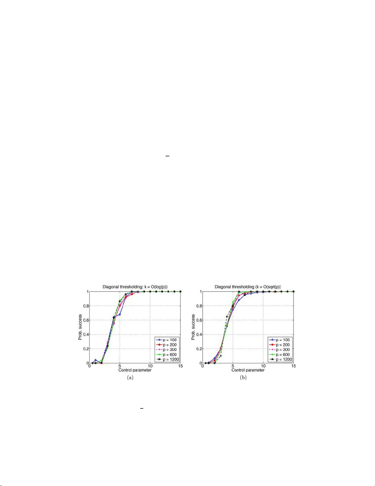
The Annals of Statistics 2009, V ol. 37, No. 5B, 2877–2 921 DOI: 10.1214 /08-A OS664 c  Institute of Mathematical Statistics , 2009 HIGH-DIMENSIONAL ANAL YSIS OF SEMIDEFINITE RELAXA TIONS F OR SP ARSE PRINCIP AL COMPONENTS 1 By Arash A. Amini and Mar tin J. W ainwright University of California, Berkeley Principal component analysis (PCA) is a classica l meth od for dimensionalit y reduction based on extracting the dominant eig env ec- tors of the sample cov ariance matrix. How ever, PCA is well known to b eha ve p o orly in the “large p , small n ” setting, in which the problem dimension p is comparable to or larger than the sample size n . This pap er studies PCA in this h igh-d imensional regime, but under the additional assumption that the maximal eigen vector is sparse, say , with at most k nonzero comp onents. W e consider a spiked cov ari- ance mo del in which a base matrix is p erturb ed by adding a k -sp arse maximal eigenv ector, and we analyze tw o computationally tractable method s for reco vering the supp ort set of this maximal eigenv ec- tor, as follow s: (a) a simple diagonal th resholding metho d, which transitions from success to failure as a function of the rescaled sam- ple size θ dia ( n, p, k ) = n/ [ k 2 log( p − k ) ]; and (b) a more sophisticated semideﬁnite programming ( SDP) relaxation, which succeeds once th e rescaled sample size θ sdp ( n, p, k ) = n/ [ k log( p − k )] is larger t han a critical t hreshold. I n add ition, w e pro ve that no metho d, including the b est method which has exp onential -time complexity , can succeed in reco vering the supp ort if the order p arameter θ sdp ( n, p, k ) is b e- lo w a threshold. Our results thus highligh t an interesting trade-oﬀ b etw een computational and statistical eﬃciency in high-dimensional inference. 1. In tro d uction. Principal comp onent analysis (PCA) is a classical metho d [ 1 , 22 ] for reducing the dimension of data, sa y , from some high-dimensional subset of R p do wn to some s u bset of R d , with d ≪ p . Principal comp onen t analysis op erates b y pro jecting the data onto the d directions of maximal Received March 2008; revised August 2008. 1 Supp orted in part by NSF Grants CAREER- CCF-05-4586 2 and D MS- 06-05165 , and a Sloan F oundation F ello wship. AMS 2000 subje ct classiﬁc ations. Primary 62H25; secondary 62F12. Key wor ds and phr ases. Principal comp onent analysis, sp ectral analysis, spik ed cov ari- ance en sembles, sparsity , high-dimensional statistics, conve x relaxation, semideﬁnite pro- gramming, Wishart ensem bles, random matrices. This is an electro nic reprint of the or iginal article published by the Institute of Mathematical Statistics in The Annals of St atistics , 2009, V ol. 37, No. 5 B, 2877 –2921 . This re print diﬀers from the original in pagination and typographic detail. 1 2 A. A. AMINI AND M. J. W AINWRIGHT v ariance, as captured by eigen vect ors of the p × p p opulation co v ariance m a- trix Σ . Of course, in p ractice, one d o es n ot hav e access to the p opulation co v ariance, but instead m u st rely on a “noisy” version of the form b Σ = Σ + ∆ , (1) where ∆ = ∆ n denotes a random noise matrix, typic ally arising from ha ving only a ﬁnite num b er n of samp les. A natural qu estion in assessing the p erfor- mance of PCA is un d er wh at conditions th e samp le eigen ve ctors (i.e., based on b Σ) are consisten t estimators of their p opulation analogues. In the classi- cal theory of PCA, the mo del dimension p is view ed as ﬁ xed, and asymptotic statemen ts are established as the num b er of observ ations n tends to inﬁnit y . With this scaling, the inﬂuence of the noise matrix ∆ d ies oﬀ, so that sam- ple eigen v ectors and eigen v alues are consisten t estimato rs of their p opulation analogues [ 1 ]. How ev er, suc h “ﬁxed p , large n ” scaling ma y b e in appropri- ate for man y con temp orary applications in science and engineering (e.g., ﬁnancial time series, astronomical imaging, sensor net works), in whic h the mo del dimension p is comparable or ev en larger than the num b er of observ a- tions n . This t yp e of h igh-dimen s ional scaling causes d ramatic br eakdo wns in standard PCA and related eigen vect or metho ds , as sh o wn b y classical and ongoing work in rand om matrix theory [ 13 , 20 , 21 ]. Without further restrictions, there is little hop e of p erforming high-dimensional inference with v ery limited data. How ev er, man y data sets exhibit add itional structure, wh ic h can partially mitigate the cur s e of dimensionalit y . One nat- ural structural assumption is that of sparsit y , and v arious t yp es of sparse mo dels hav e b een stu died in past statistica l work. There is a sub stan tial and on-going line of w ork on subset selection and sp arse regression mo dels (e.g., [ 6 , 11 , 28 , 35 , 36 ]), fo cusing in particular on the b eha vior of v arious ℓ 1 -based rela xation metho d s. Other w ork has tac kled the problem of es- timating sparse co v ariance matrices in the high-dimensional setting, us in g thresholding metho ds [ 3 , 12 ] as w ell as ℓ 1 -regularizati on metho ds [ 8 , 39 ]. A related problem—and the primary f o cus of this pap er—is reco ve ring sparse eigen v ectors fr om high-dimensional data. While related to sparse co- v ariance estimation, the sparse eigen vec tor problem p resen ts a diﬀeren t set of c hallenges; indeed, a co v ariance m atrix may hav e a sparse eigen v ector with neither it nor its in verse b eing a sparse matrix. V arious researc hers ha ve prop osed metho ds for extracting sp arse eigen v ectors, a p roblem often referred to as sparse pr incipal comp onent analysis (SP CA). Some of these metho ds are based on greedy or nonconv ex optimization pro cedures (e.g., [ 23 , 29 , 40 ]), w hereas others are based on v arious types of ℓ 1 -regularizati on [ 9 , 41 ]. Zou, Hastie and Tibshirani [ 41 ] deve lop a metho d b ased on transform- ing the PCA problem to a r egression problem and then applying the Lasso ANAL YSIS OF SEMIDEFINITE RELA X A TION S 3 ( ℓ 1 -regularizati on). Johnstone and Lu [ 21 ] prop osed a t wo-ste p metho d , u s- ing an initial pr e-pro cessing step to select relev an t v ariables follo w ed by or- dinary PCA in the reduced sp ace. Under a p articular ℓ q -ball sparsit y mo d el, they pro ved ℓ 2 -consistency of their pro cedure as long as p/n conv erges to a constan t. In recent work, d ’Aspr ´ emon t et al. [ 9 ] ha v e form ulated a di- rect semideﬁn ite programming (SDP) relaxation of the s parse eigen v ector problem, and dev elop ed fast algorithms for solving it, but ha v e not pro- vided high-dimens ional consistency results. The elegan t work of Pa ul and Johnstone [ 30 , 32 ], br ou ght to our atten tion after initial subm ission, studies estimatio n of eigen v ectors satisfying wea k ℓ q -ball s parsit y assu m ptions f or q ∈ (0 , 2). W e discuss connections to this work at more length b elo w. In this pap er, we stud y the mo del selection problem for sparse eigen vec- tors. More precisely , we consider a sp ik ed co v ariance mo del [ 20 ], in whic h the maximal eigen vec tor z ∗ of the p opu lation cov ariance Σ p ∈ R p × p is k -sparse, meaning that it has n onzero en tries on a su bset S ( z ∗ ) with cardinalit y k , and our goal is to reco ver this supp ort set exactly . In order to do so, we ha ve access to a matrix b Σ, r ep r esen ting a noisy version of the p opulation co v ari- ance, as in ( 1 ). Although our theory is somewhat more generally applicable, the most n atural instan tiation of b Σ is as a samp le cov ariance matrix based on n i.i.d. samples d ra w n from the p opulation. W e analyze this setup in the high-dimensional regime, in which all three parameters—the n u mb er of ob- serv ations n , the am bien t dimension p and the sparsit y index k —are allo w ed to tend to inﬁn it y simulta neously . Our primary in terest is in the follo wing question: usin g a giv en inf erence pro cedure, u nder what conditions on the scaling of triplet ( n, p, k ) is it p ossible, or con ve rsely imp ossible, to r eco v er the sup p ort set of the maximal eigen v ector z ∗ with probabilit y one? W e pro vide a detailed analysis of t w o p r o cedures for r eco v ering sparse eigen v ectors, as follo ws: (a) a simple diagonal thresh olding metho d, used as a pre-pro cessing step by Johnstone and Lu [ 21 ], and (b) a semideﬁ- nite programming (SDP) relaxation for sparse PC A, recent ly dev elop ed b y d’Aspremont et al. [ 9 ]. Un der the k -sparsit y assumption on the maximal eigen v ector, we p r o ve that th e success or failure p robabilities of these tw o metho ds ha ve qualitativ ely d iﬀeren t scaling in terms of the triplet ( n, p, k ) . F or th e diagonal thresholding metho d, we prov e that its success or failure is go v erned by the rescaled sample size θ dia ( n, p, k ) := n k 2 log( p − k ) , (2) meaning that it succeeds with pr ob ability one for scalings of the triplet ( n, p, k ) such that θ dia is ab o ve some critical v alue and , con v ersely , fails with probabilit y one when this ratio falls b elo w some critical v alue. W e then establish p erformance guarant ees for the SDP relaxation [ 9 ]. In particular, 4 A. A. AMINI AND M. J. W AINWRIGHT for the same class of mo dels, we s h o w that it alwa ys has a unique rank- one solution that sp eciﬁes the co rrect signed sup p ort once θ dia ( n, p, k ) is suﬃcien tly large, moreo ver, that for su ﬃ cien tly large v alues of the r escaled sample size θ sdp ( n, p, k ) := n k log ( p − k ) , (3) if there exists a rank-one solution, then it sp eciﬁes the correct signed su pp ort. The pro of of this resu lt is based on random m atrix theory , concen tration of measure and Gaussian comparison inequalities. O ur ﬁnal con tribution is to use inform ation-theoretic argumen ts to sho w that no metho d can succeed in reco v ering the signed su pp ort f or the spike d identit y co v ariance mo del if the order parameter θ sdp ( n, p, k ) lies b elo w some critical v alue. O ne consequence is that the give n scaling ( 3 ) for th e S DP relaxation is s h arp, meaning the SDP relaxatio n also fails once θ sdp drops b elo w a critical thresh old. Moreo v er, it sho w s th at un d er the r ank-one condition, the SDP is in fact statistical ly optimal, that is, it r equires only the necessary num b er of samples (u p to a constan t factor) to succeed. The results rep orted here are complemen tary to those of Paul and John- stone [ 30 , 32 ], wh o prop ose and analyze the augmen ted SPCA algorithm f or estimating eigen ve ctors. In comparison to the mo dels analyzed here, their analysis app lies to spike d m o dels us in g the id en tit y base co v ariance, b ut it al- lo ws for m > 1 eigen v ectors in the sp iking. In addition, they consider the class of w eak ℓ q -ball s parsit y mo dels, as opp osed to the h ard ℓ 0 -sparsit y mo del considered here. Another diﬀerence is that their results provide guarantee s in terms of the ℓ 2 -norm b et wee n the eigen v ector and its estimate, wh ereas our results guaran tee exact sup p ort reco very . W e note that an estimate can b e close in ℓ 2 -norm wh ile h a ving a very d iﬀeren t supp ort set. Consequentl y , the results giv en here, w hic h pro vid e conditions for exact supp ort reco very , pro vide complemen tary insight. Our results highligh t some in teresting trade-oﬀs b et ween computational and statistical costs in high-dimensional inference. On one hand , the sta- tistical eﬃciency of SDP relaxation is su bstan tially greater than the diag- onal thresholding metho d , requiring O (1 /k ) few er observ ations to succeed. Ho wev er, the computational complexit y of S DP is also larger by roughly a factor O ( p 3 ). An implemen tation due to d’Aspr´ emon t et al. [ 9 ] has com- plexit y O ( np + p 4 log p ) as opp osed to the O ( np + p log p ) complexit y of the diagonal th r esholding metho d. Moreo v er, our information-theoreti c analysis sho w s that the b est p ossible metho d—n amely , one based on an exhaustiv e searc h o ver all  p k  subsets, with exp onent ial complexit y—do es not ha v e sub- stan tially greater statistical eﬃciency than the SDP relaxation. The remaind er of this pap er is organized as follo ws. In Section 2 , w e pro vide precise statemen ts of our main results, discuss some of their impli- cations and pro vide sim ulation resu lts to illustrate the sharpness of their ANAL YSIS OF SEMIDEFINITE RELA X A TION S 5 predictions. Sections 3 , 4 and 5 are dev oted to pro ofs of these results, with some of the more tec hnical asp ects deferred to app endices. W e conclude in Section 6 . 1.1. Notation. F or the reader’s con venience, we state here some notation used throughout the p ap er. F or a v ector x ∈ R n , w e use k x k p = ( P n i =1 | x i | p ) 1 /p to denote its ℓ p -norm. F or a matrix A ∈ R m × n , w e u s e | | | A | | | p,q to denote the matrix op erator norm induced by v ector norms ℓ p and ℓ q ; more precisely , w e ha v e | | | A | | | p,q := max k x k q =1 k Ax k p . (4) A few cases of particular in terest in this pap er are (a) the sp e ctr al norm giv en by | | | A | | | 2 , 2 := max i =1 ,...,m { σ i ( A ) } , where { σ i ( A ) } are the singular v alues of A , and the ℓ ∞ -op er ator norm , giv en b y | | | A | | | ∞ , ∞ := max i =1 ,...,m n X j =1 | A ij | . Giv en t w o square matrices X , Y ∈ R n × n , we deﬁne the matrix inn er pro d uct h h X, Y i i := tr( X Y T ) = P i,j X ij Y ij . Note that this inner pr o duct induces the Hilb ert–Sc hm idt norm | | | X | | | HS = p h h X, X i i . W e use the follo wing standard asymptotic notation: for fu nctions f , g , the notation f ( n ) = O ( g ( n )) means that there exists a ﬁxed constan t 0 < C < + ∞ such th at f ( n ) ≤ C g ( n ) ; the notation f ( n ) = Ω( g ( n )) means that f ( n ) ≥ C g ( n ), and f ( n ) = Θ( g ( n )) means that f ( n ) = O ( g ( n )) and f ( n ) = Ω( g ( n )). Note in particular that wh en used w ithout a subs crip t “ p ,” these sym b ols are to b e in terpr eted in a deterministic sense, that is, the constan ts in volv ed are assumed to b e n onrandom. W e use λ ( A ) to denote a generic eigen v alue of a square matrix A , as w ell as λ min ( · ) and λ max ( · ) for the minimal and the maximal eigen v alues, resp ectiv ely . An y mem b er of the set of eigen v ectors of A asso ciated with an eigen v alue is den oted as ~ v ( A ). Thus, ~ v max ( · ), f or example, repr esen ts the eigen vec tors asso ciated with the maximal eigen v alue (o ccasionally re- ferred to as “maximal eigen v ectors”). W e alw ays assum e that eigen v ectors are norm alized to un it ℓ 2 -norm and ha ve a n onnegativ e ﬁ rst comp onent. The sign con ve n tion guarante es uniquen ess of the eigen v ector asso ciated with an eigen v alue with geometric multiplicit y one. Finally , some probabilistic notation: w e say a sequence of eve n ts { E j } j ≥ 1 happ ens with asymptotic probabilit y one (w.a.p. one) if lim j → + ∞ P [ E j ] = 1, whereas it holds asymptot ically almo st surely (a.a.s.) as j → + ∞ if P (lim inf E j ) = 1 . 6 A. A. AMINI AND M. J. W AINWRIGHT 2. Main resu lts and consequences. The primary fo cus of this pap er is the spike d c ovarianc e mo del , in wh ich some b ase co v ariance matrix is p ertur b ed b y the addition of a sparse eigen vect or z ∗ ∈ R p . I n particular, w e study sequences of co v ariance matrices of the form Σ p = β z ∗ z ∗ T +  I k 0 0 Γ p − k  = β z ∗ z ∗ T + Γ , (5) where Γ p − k ∈ S p − k + is a symmetric PS D matrix w ith λ max (Γ p − k ) ≤ 1. Note that we hav e assumed (without loss of generalit y , by re-ordering the indices as necessary) that the nonzero en tries of z ∗ are indexed by { 1 , . . . , k } , so that ( 5 ) is the form of the co v ariance after an y re-ordering. W e also assume that the nonzero part of z ∗ has en tries z ∗ i ∈ 1 √ k {− 1 , +1 } , so th at k z ∗ k 2 = 1. The sp ik ed co v ariance m o del ( 5 ) w as ﬁ rst p r op osed by Johnstone [ 20 ], who fo cused on the spiked iden tit y co v ariance matrix [i.e., mo del ( 5 ) with Γ p − k = I p − k ]. John stone and Lu [ 21 ] established that the sample eigen v ectors for the spik ed iden tit y mo del, b ased on a set of n i.i.d. samples with distribution N (0 , Σ p ) from the sp ik ed ident it y ensemble, are inconsisten t as estimato rs of z ∗ i whenev er p/n → c > 0. T hese asymptotic results were reﬁned b y later w ork [ 2 , 31 ]. In this p ap er, w e stud y a slight ly more general family of spik ed cov ari- ance mo d els, in whic h the m atrix Γ p − k is required to satisfy the follo wing conditions: A1. | | | q Γ p − k | | | ∞ , ∞ = O (1) and (6a) A2. λ max (Γ p − k ) ≤ min  1 , λ min (Γ p − k ) + β 8  . (6b) Here p Γ p − k denotes the sym metric square ro ot. These conditions are triv- ially satisﬁed b y the iden tit y matrix I p − k , but also can hold for more general nondiagonal matrices. T h us, under th e mo del ( 5 ), the p opulation co v ari- ance m atrix Σ itself need not b e sparse, since (at least generically) it h as k 2 + ( p − k ) 2 = Θ( p 2 ) nonzero entries. Assumption (A2) on th e eigensp ectrum of the matrix Γ p − k ensures that as long as β > 0, then the v ector z ∗ is the unique maximal eigen ve ctor of Σ , with asso ciated eigenv alue (1 + β ). Since the remaining eigen v alues are b ounded ab o v e b y 1, the p arameter β > 0 represen ts a signal-to-noise ratio, c haracterizing the separation b et ween th e maximal eigen v alue and the remainder of the eigensp ectrum. Assump tion (A1) is related to the fact that reco v ering the correct signed sup p ort means that the estimate b z must satisfy k b z − z ∗ k ∞ ≤ 1 / √ k . As will b e clariﬁed by our an alysis (see Section 4.4 ), con trolling this ℓ ∞ -norm r equires b ounds on terms of the form k p Γ p − k u k ∞ , whic h requires con trol of the ℓ ∞ -op erator norm | | | p Γ p − k | | | ∞ , ∞ . ANAL YSIS OF SEMIDEFINITE RELA X A TION S 7 In th is p ap er, we study the mo del sele ction pr oblem for eigen v ectors: that is, we assum e that the maximal eigen vec tor z ∗ is k -sparse, m eaning that it has exactly k n onzero entrie s, and our goal is to r eco v er this supp ort, along with the sign of z ∗ on its supp ort. W e let S ( z ∗ ) = { i | z ∗ i 6 = 0 } denote the su pp ort set of the maximal eigen v ector; recall that S ( z ∗ ) = { 1 , . . . , k } b y ou r assumed ordering of the indices. Moreo v er, we deﬁne the fun ction S ± : R p → {− 1 , 0 , +1 } p b y [ S ± ( u )] i :=  sign( u i ) , if u i 6 = 0, 0 , otherwise, (7) so that S ± ( z ∗ ) enco des the signe d supp ort of the maximal eigen v ector. Giv en some estimate c S ± of the true signed sup p ort S ± ( z ∗ ), w e assess it based on the 0–1 loss I [ c S ± 6 = S ± ( z ∗ )], so that the asso ciated risk is simply the probabilit y of incorrect d ecision P [ c S ± 6 = S ± ( z ∗ )]. Our goal is to sp ecify con- ditions on the scaling of the triplet ( n, p , k ) suc h that this error probabilit y v anishes, or con versel y , fails to v anish asymptotically . W e consider metho ds that op erate based on a set of n samples x 1 , . . . , x n , dr a wn i.i.d. with dis- tribution N (0 , Σ p ). Und er the sp ik ed co v ariance mo del ( 5 ), eac h sample can b e wr itten as x i = p β v i z ∗ + √ Γ g i , (8) where √ Γ is the symmetric matrix square ro ot. Here v i ∼ N (0 , 1) is stand ard Gaussian, and g i ∼ N (0 , I p × p ) is a standard Gaussian p -v ector, indep enden t of v i , so th at √ Γ g i ∼ N (0 , Γ). T he data { x i } n i =1 deﬁnes the sample co v ariance matrix b Σ := 1 n n X i =1 ( x i )( x i ) T , (9) whic h follo ws a p -v ariate Wishart distrib ution [ 1 ]. In this pap er, w e analyze the high-dimensional scaling of t wo metho d s f or r eco v ering the signed sup - p ort of the maximal eigen v ector. It will b e assu med throughout that the size k of the s u pp ort of z ∗ is a v ailable to the metho ds a pr iori, that is, we do not mak e any attempt at estimating k . 2.1. Diagonal thr esholding metho d. Under the spik ed co v ariance mo del ( 5 ), note that the diagonal elemen ts of the p opulation co v ariance sat isfy Σ ℓℓ = 1 + β /k for all ℓ ∈ S , and Σ ℓℓ ≤ 1 for all ℓ / ∈ S . (This latter b ound follo ws since for all ℓ / ∈ S , we ha ve Σ ℓℓ ≤ | | | Γ p − k | | | 2 , 2 ≤ 1.) This observ ation motiv ates a natural approac h to reco v ering information ab out the su pp ort set S , previously used as a p re-pro cessing step b y Johnstone and Lu [ 21 ]. 8 A. A. AMINI AND M. J. W AINWRIGHT Let D ℓ , ℓ = 1 , . . . , p , b e the diagonal elemen ts of the sample co v ariance matrix—namely , D ℓ = 1 n n X i =1 ( x i ℓ ) 2 = [ b Σ] ℓℓ . F orm the asso ciated order statistics D (1) ≤ D (2) ≤ · · · ≤ D ( p − 1) ≤ D ( p ) , and output the rand om sub set b S ( D ) of cardinalit y k sp eciﬁed b y the in- dices of the largest k elements { D ( p − k +1) , . . . , D ( p ) } . The chief app eal of this metho d is its low compu tational complexit y . Ap art from the order O ( np ) of computing the diagonal elemen ts of b Σ, it requires only p erforming a sorting op eration, with complexit y O ( p log p ). Note that this metho d pr o vides only an estimate of the su pp ort S ( z ∗ ), as opp osed to the signed supp ort S ± ( z ∗ ). O ne could imagine extending the metho d to extract sign in formation as w ell, but our main int erest in studyin g this m etho d is to pro vide a simple b enc hmark by whic h to calibrate our later r esults on the p erformance of the more complex SDP relaxation. In particular, the follo wing result pro vides a p recise c haracteriza tion of the statistic al b ehavio r of the diagonal thresholding metho d. Pr oposition 1 (P erformance of diagonal th r esholding). F or k = O ( p 1 − δ ) for any δ ∈ (0 , 1) , the pr ob ability of suc c essful r e c overy u sing diagonal thr esh- olding under go es a phase tr ansition as a function of the r esc ale d sample size θ dia ( n, p, k ) = n k 2 log( p − k ) . (10) Mor e pr e cisely, ther e exists a c onstant θ u such that if n > θ u k 2 log( p − k ) , then P [ b S ( D ) = S ( z ∗ )] ≥ 1 − exp( − Θ( k 2 log( p − k ))) → 1 , (11) so that the metho d suc c e e ds w.a.p. one and a c onstant θ ℓ > 0 such that if n ≤ θ ℓ k 2 log( p − k ) , then P [ b S ( D ) = S ( z ∗ )] ≤ exp( − Θ(log ( p − k ))) → 0 , (12) so that the metho d fails w.a.p. one. Remarks. The pro of of Pr op osition 1 , pro vided in Section 3 , is b ased on large d eviatio ns b oun ds on χ 2 -v ariates. The ac hiev abilit y assertion ( 11 ) uses kno wn upp er b oun d s on the tails of χ 2 -v ariates (e.g., [ 4 , 21 ]). The con ve rse result ( 12 ) requires an exp onentia lly tigh t lo wer b oun d on the tails of χ 2 -v ariates, whic h w e derive in App endix C . ANAL YSIS OF SEMIDEFINITE RELA X A TION S 9 T o ill ustrate the prediction of Prop osition 1 , w e p ro vide some results on the diagonal th resholding metho d. F or all experiments rep orted here, w e generated n samples { x 1 , . . . , x n } in an i.i.d. manner from the spik ed co v ariance ensem b le ( 5 ), with Γ = I and β = 3 . Figure 1 illustrates the b e- ha vior pr edicted b y Prop osition 1 . Each panel p lots the success probabilit y P [ b S ( D ) = S ( z ∗ )] versus the rescaled sample size θ dia ( n, p, n ) = n/ [ k 2 log( p − k )]. Eac h pan el sho w s ﬁve mo del dimensions ( p ∈ { 100 , 20 0 , 300 , 600 , 1200 } ), with panel (a) sho w ing the logarithmic sp ars ity ind ex k = O (log p ) and p anel (b) sh o wing the case k = O ( √ p ). Eac h p oint on eac h curve corresp onds to the av erage of 100 indep endent trials. As predicted b y Prop osition 1 , the curv es all coincide, ev en though they corresp ond to v ery diﬀeren t regimes of ( p, k ). 2.2. Semideﬁnite-pr o gr amming r elaxation. W e no w describ e the approac h to s p arse PC A dev elop ed by d ’Aspr´ e mon t et al. [ 9 ]. Let S p + = { Z ∈ R p × p | Z = Z T , Z  0 } d enote the cone of symmetric, p ositiv e semideﬁn ite (PSD) matrices. Giv en n i.i.d. observ ations f rom the mo del N (0 , Σ p ), let b Σ b e the sample co v ariance matrix ( 9 ), and let ρ n > 0 b e a user-deﬁned regulariza- tion parameter. d’Aspr´ emon t et al. [ 9 ] pr op ose estimating z ∗ b y solving the optimizatio n pr oblem b Z := arg max Z ∈ S p +  tr( b Σ Z ) − ρ n X i,j | Z ij |  s.t. tr( Z ) = 1, (13) Fig. 1. Plot of the suc c ess pr ob ability P [ b S ( D ) = S ( z ∗ )] versus the r esc ale d sample size θ dia ( n, p, k ) = n/ [ k 2 log( p − k ) ] . T he ﬁve curves in e ach p anel c orr esp ond to mo del dimen- sions p ∈ { 100 , 200 , 300 , 600 , 1200 } , SNR p ar ameter β = 3 and sp arsity indic es k = O (log p ) in p anel (a) and k = O ( √ p ) i n p anel (b) . As pr e dicte d by Pr op osition 1 , the suc c ess pr ob- ability under go es a phase tr ansition, wi th the curves for diﬀer ent mo del sizes and diﬀer ent sp arsity i ndic es al l lying on top of one another. 10 A. A. AMINI AND M. J. W AINWRIGHT and computing the maximal eigen v ector b z = ~ v max ( b Z ). T he optimization problem ( 13 ) is a semideﬁn ite p rogram (SDP), a class of con ve x conic pro- grams that can b e solv ed exactly in p olynomial time. Indeed, d’Aspr´ emon t et al. [ 9 ] describ e an O ( p 4 log p ) algorithm, with an implementa tion p osted online, that we use for all simulat ions rep orted in th is pap er. T o gain s ome in tuition for th e SDP relaxation ( 13 ), recall the follo wing Couran t–Fisc her v ariational represent ation [ 18 ] of the maximal eigen v alue and eigen vect or: ~ v max ( b Σ) = arg max k z k 2 =1 z T b Σ z . (14) A lesser kno w n bu t equiv alen t v ariational represent ation is in terms of th e semideﬁnite pr ogram (SDP) Z ∗ = arg max Z ∈ S p + , tr( Z )=1 tr( b Σ Z ) . ( 15) F or this p roblem, if the maximal eigen v alue is s imp le, the optim um is alw a ys ac hiev ed at a rank-one matrix Z ∗ = z ∗ ( z ∗ ) T , wh ere z ∗ = ~ v max ( b Σ) is th e max- imal eigen ve ctor; otherwise, there exist optimal solutions of higher rank, bu t the optim um is alw ays ac hiev ed by at least some rank-one matrix. If we we re giv en a priori information that the maximal eigen vec tor were sparse, then it migh t b e natural to solv e the same s emid eﬁ n ite program with the add i- tion of an ℓ 0 constrain t. Giv en the intracta bilit y of suc h an ℓ 0 -optimizat ion problem, the SDP program ( 13 ) is a natural r elaxati on. In p articular, the follo wing result pro vides su ﬃcien t conditions for the SDP relaxation ( 13 ) to succeed in reco ve ring th e correct signed supp ort of the maximal eigenv ector. Theorem 2 (SDP p erf orm ance guarantee s). Imp ose c onditions ( 6a ) and ( 6b ) on the se que nc e of p opulation c ovarianc e matric es { Σ p } , and sup- p ose mor e over that ρ n = β / (2 k ) and k = O (log p ) . Then: (a) Rank guaran tee: ther e exists a c onstant θ wr = θ wr (Γ , β ) suc h that for al l se quenc es ( n, p, k ) satisfying θ dia ( n, p, k ) > θ wr , the semideﬁnite pr o gr am ( 13 ) has a r ank-one solution with high pr ob ability. (b) Critical s caling: ther e exists a c onstant θ crit = θ crit (Γ , β ) such that if the se quenc e ( n, p, k ) satisﬁes θ sdp ( n, p, k ) := n k log ( p − k ) > θ crit (16) and if ther e exists a r ank-one solution, then it sp e ciﬁes the c orr e ct signe d supp ort with pr ob ability c onver ging to one. ANAL YSIS OF SEMIDEFINITE RELA X A TION S 11 Remarks. P art (a) of the theorem shows that rank-one solutions of the SDP ( 13 ) are not uncommon; in particular, they are guaran teed to ex- ist with high p robabilit y at least u nder the weak er scaling of the diagonal thresholding metho d. The main contribution of Theorem 2 is its p art (b), whic h pro vides su ﬃcien t conditions for signed su pp ort reco very using the SDP , when a rank-one solution exists. The bulk of our tec hn ical eﬀort is dev oted to part (b); indeed, the pro of of part (a) is straigh tforwa rd once all the p ieces of the pro of of part (b) hav e b een in tr o duced, and so will b e deferred to App endix G . F or tec hnical reasons, our cur ren t pro of(s) require the condition k = O (log p ) ; h o wev er, it should b e p ossible to r emo ve this restriction, and indeed, the empirical results do not app ear to require it. Prop osition 1 and Th eorem 2 apply to the p erformance of sp eciﬁc (p olynomial- time) metho ds. It is natural then to ask wh ether there exists an y algorithm, p ossibly with su p er-p olynomial complexit y , that has greater statistical eﬃ- ciency . The follo wing result is information-theoretic in n atur e, and c h arac- terizes the fundament al limitations of an y algorithm regardless of its com- putational complexit y . Theorem 3 (Information-theoretic limitat ions). Consider the pr oblem of r e c overing the eigenve ctor supp ort in the spike d c ovarianc e mo del ( 5 ) with Γ = I p . F or any se quenc e ( n, p, k ) → + ∞ such that θ sdp ( n, p, k ) := n k log ( p − k ) < 1 + β β 2 , (17) the pr ob ability of e rr or of any metho d i s at le ast 1 / 2 . Remarks. T oget her with Theorem 2 , this result establishes the sharp - ness of the th reshold ( 16 ) in c haracterizing the b eha vior of SDP relaxation, and moreo v er, it guaran tees optimalit y of the SDP scaling ( 16 ), up to con- stan t factors, for the spiked identit y ensemble. T o illustrate the predictions of Theorem 2 and 3 , w e applied the S DP relaxatio n to the spik ed iden tit y co v ariance ensem ble, again generating n i.i.d. samples. W e solv ed the SDP relaxation us ing p ublically a v ailable co de pro vided by d’Aspr´ emon t et al. [ 9 ]. Figure 2 sho ws the corresp onding p lots for the S DP relaxati on [ 9 ]. Here we plot the prob ability P [ S ± ( b z ) = S ± ( z ∗ )] that the SDP relaxation correctly reco v ers the signed supp ort of the un- kno wn eigen v ector z ∗ , wh ere the signs are c hosen uniformly in {− 1 , +1 } at random. F ollo w ing Theorem 2 , the horizon tal axis plots the rescaled sample size θ sdp ( n, p, k ) = n / [ k log( p − k )] . Eac h panel s h o ws p lots f or thr ee diﬀer- en t problem sizes, p ∈ { 100 , 200 , 300 } , with panel (a) corresp ondin g to log- arithmic s parsit y [ k = O (log p )], and panel (b) to linear sparsity ( k = 0 . 1 p ). 12 A. A. AMINI AND M. J. W AINWRIGHT Fig. 2. Pe rformanc e of the SDP r elaxation f or the spike d identity ensemble, plotting the suc c ess pr ob abil ity P [ S ± ( b z ) = S ± ( z ∗ )] versus the r esc ale d sample size θ sdp ( n, p, k ) = n/ [ k log( p − k ) ] . The thr e e curves in e ach p anel c orr esp ond to mo del di- mensions p ∈ { 100 , 200 , 300 } , SNR p ar ameter β = 3 and sp arsity indic es k = O (log p ) in p anel (a) and k = 0 . 1 p in p anel (b ) . As pr e dicte d by The or em 2 , the curves in p anel (a) al l li e on top of one another, and tr ansition to suc c ess onc e the or der p ar ameter θ sdp is suﬃciently lar ge. Consisten t with the prediction of T heorem 2 , the success probabilit y rapidly approac hes one once the rescaled sample size exceeds some critical threshold. [Strictly sp eaking, Theorem 2 only co ve rs the case of logarithmic sparsity sho w n in panel (a), b ut the linear sparsit y curves in panel (b) sho w the same qualitativ e b ehavio r.] Note that this empirical b eha vior is consisten t with our conclusion that the order p arameter θ sdp ( n, p, k ) = n/ [ k log ( p − k )] is a sharp d escription of the S DP threshold. 3. Pro of of Prop osition 1 . W e b egin by proving th e ac hiev abilit y result ( 11 ). W e pro vide a detailed pro of for the case Γ p − k = I p − k and discuss nec- essary mo d iﬁ cations for th e general case at the end. F or ℓ = 1 , . . . , p , w e ha ve D ℓ = 1 n n X i =1 ( x i ℓ ) 2 = 1 n n X i =1 [ p β z ∗ ℓ v i + g i ℓ ] 2 . (18) Since ( √ β z ∗ ℓ v i + g i ℓ ) ∼ N (0 , β ( z ∗ ℓ ) 2 + 1) for eac h i , the rescaled v ariate n β ( z ∗ ℓ ) 2 +1 × D ℓ is cen tral χ 2 n with n degrees of freedom. Consequent ly , we hav e E [ D ℓ ] = ( 1 , for all ℓ ∈ S c , 1 + β k , for all ℓ ∈ S , where we h a ve used the fact that ( z ∗ ℓ ) 2 = 1 /k for ℓ ∈ S , by assumption. ANAL YSIS OF SEMIDEFINITE RELA X A TION S 13 A suﬃcien t condition for success of the diagonal thresholding deco der is a thresh old τ k suc h that D ℓ ≥ (1 + τ k ) for all ℓ ∈ S , and D ℓ < (1 + τ k ) for all ℓ ∈ S c . Using the u nion b ound and the tail b ound ( 61 ) on cent ral χ 2 , we ha ve P h max ℓ ∈ S c D ℓ ≥ (1 + τ k ) i ≤ ( p − k ) P  χ 2 n n ≥ 1 + τ k  ≤ ( p − k ) exp  − 3 n 16 τ 2 k  , so that the probabilit y of false inclusion v anishes as long as n > 16 3 ( τ k ) − 2 × log( p − k ). On the other h and, using the union b ound and th e tail b ound ( 60b ), w e ha ve P h min ℓ ∈ S D ℓ < (1 + τ k ) i ≤ k P  χ 2 n n − 1 < 1 + τ k 1 + β /k − 1  = k P  χ 2 n n − 1 < τ k − β /k 1 + β /k  ≤ k P  χ 2 n n − 1 < τ k − β k  . As long as τ k < β /k , w e ma y choose x = n 4 ( β k − τ k ) 2 in ( 60b ), thereb y ob- taining the upp er b oun d P h min ℓ ∈ S D ℓ < n (1 + τ k ) i ≤ k exp  − n 4  β k − τ k  2  , so that the p robabilit y of false exclusion v anishes as long as n > 4 ( β /k − τ k ) 2 log k . Ov erall, c h o osing τ k = β 2 k ensures that the probabilit y of b oth types of error v anish asymptotically as long as n > max  64 3 β 2 k 2 log( p − k ) , 16 β 2 k 2 log k  . Since k = o ( p ), the log ( p − k ) term is the dominant r equiremen t. The mo d - iﬁcations required for the case of general Γ p − k are straigh tforward. Since v ar( √ Γ g i ) ℓ = (Γ p − k ) ℓℓ ≤ 1 f or all ℓ ∈ S c and samp les i = 1 , . . . , n , we n eed to adju st the scaling of the χ 2 n v ariates. F or general Γ p − k , the v ariates { D ℓ , ℓ ∈ S c } need no longer b e indep endent, but our pro of used only u nion b ound , and so is v alid r egardless of the dep endence stru cture. W e no w pr o ve the con v erse claim ( 12 ) for the spik ed iden tit y ensemble. A t a high lev el, this p ortion of the pr o of consists of the follo wing steps. F or a p ositiv e r eal t , d eﬁne the eve n ts A 1 ( t ) := n max ℓ ∈ S c D ℓ > 1 + t o and A 2 ( t ) := n min ℓ ∈ S D ℓ < 1 + t o . Noting that the even t A 1 ( t ) ∩ A 2 ( t ) implies failure of the diagonal cutoﬀ deco der, it suﬃ ces to sh o w the existence of some t > 0 suc h that P [ A 1 ( t )] → 1 and P [ A 2 ( t )] → 1. 14 A. A. AMINI AND M. J. W AINWRIGHT Ana lysis of eve nt A 1 ( t ) . Cen tral to the analysis of ev en t A 1 is the fol- lo wing large-deviatio ns lower b ound on χ 2 -v ariates. Lemma 4. F or a c entr al χ 2 n variable with n de gr e es of fr e e dom, ther e exists a c onstant C > 0 such that P  χ 2 n n > 1 + t  ≥ C √ n exp( − nt 2 / 2) for al l t ∈ (0 , 1) . See App endix C for the pro of. W e exploit this lemma as follo ws. First, deﬁn e the in teger-v alued random v ariable Z ( t ) := X ℓ ∈ S c I [ D ℓ > 1 + t ] corresp onding to the num b er of indices ℓ ∈ S c for whic h the diagonal en- try D ℓ exceeds 1 + t , and note that P [ A 1 ( t )] = P [ Z ( t ) > 0]. By a one-sided Chebyshev inequalit y [ 15 ], we hav e P [ A 1 ( t )] = P [ Z ( t ) > 0] ≥ ( E [ Z ( t )] ) 2 ( E [ Z ( t )] ) 2 + v ar( Z ( t )) . (19) Note that Z ( t ) is a sum of ( p − k ) ind ep endent Bernoulli indicators, eac h with the same parameter q ( t ) := P [ D ℓ > 1 + t ] . Computing the mean E [ Z ( t )] = ( p − k ) q ( t ) and v ariance v ar( Z ( t )) = ( p − k ) q ( t )(1 − q ( t )), and then substi- tuting into the Chebyshev b ound ( 19 ), we obtain P [ A 1 ( t )] ≥ ( p − k ) 2 q 2 ( t ) ( p − k ) 2 q 2 ( t ) + ( p − k ) q ( t )(1 − q ( t )) ≥ ( p − k ) q ( t ) ( p − k ) q ( t ) + 1 ≥ 1 − 1 ( p − k ) q ( t ) . Consequen tly , the condition ( p − k ) q ( t ) → ∞ implies that P [ A 1 ( t )] → 1 . Let us set t = q δ log ( p − k ) n . [Here δ ∈ (0 , 1) is the parameter from the as- sumption k = O ( p 1 − δ ).] F rom Lemma 4 , w e ha ve q ( t ) ≥ C √ n exp( − nt 2 / 2), so that ( p − k ) q s δ log ( p − k ) n ! ≥ C ( p − k ) √ n exp  − δ 2 log( p − k )  = C ( p − k ) 1 − δ/ 2 √ n . ANAL YSIS OF SEMIDEFINITE RELA X A TION S 15 Since n ≤ Lk 2 log( p − k ) for some L < + ∞ b y assumption, we ha ve ( p − k ) q s δ log ( p − k ) n ! ≥ C √ L ( p − k ) 1 − δ k ( p − k ) δ/ 2 p log( p − k ) , whic h div erges to inﬁnit y , since k = O ( p 1 − δ ). Ana lysis of eve nt A 2 . In order to analyze this eve n t, w e ﬁ rst need to con- dition on the random vect or v := ( v 1 , . . . , v n ), so as to decouple the random v ariables { D ℓ , ℓ ∈ S } . After cond itioning on v , eac h v ariate nD ℓ , ℓ ∈ S , is a noncen tral χ 2 n,ν ∗ , with n degrees of fr eedom and noncentra lit y paramete r ν ∗ = β k k v k 2 2 , so that eac h D ℓ has mean ( ν ∗ + n ). Since v is a standard Gaussian n -vec tor, w e ha ve k v k 2 2 ∼ χ 2 n . Therefore, if we deﬁn e the ev ent B ( v ) := { k v k 2 2 n > 3 2 } , the large deviations b oun d ( 60a ) implies that P [ B ] ≤ exp( − n/ 16). Therefore, by conditioning on B and its complemen t, w e obtain P [ A c 2 ] ≤ P h min ℓ ∈ S D ℓ > 1 + t | B c i + P [ B ] (20) ≤ ( P [ χ 2 n,ν ∗ > n (1 + t ) | B c ]) k + exp( − n/ 16) , where we hav e u sed the conditional ind ep endence of { D ℓ , ℓ ∈ S } . Finally , since k v k 2 2 n ≤ 3 2 on the ev en t B c , we ha ve ν ∗ ≤ 3 β 2 k n , and th us P [ χ 2 n,ν ∗ > n (1 + t ) | B c ] ≤ P  χ 2 n,ν ∗ > { n + ν ∗ } + n  t − 3 β 2 k  | B c  . Since t = p δ log( p − k ) /n and n < Lk 2 log( p − k ), we hav e t ≥ q δ L 1 k , so that the quant it y ǫ := min { 1 2 , t − 3 β 2 k } is p ositiv e for the p r e-factor L > 0 c hosen suﬃcien tly small. T h us, we h a ve P [ χ 2 n,ν ∗ > n (1 + t ) | B c ] ≤ P [ χ 2 n,ν ∗ > { n + ν ∗ } + nǫ ] ≤ exp  − nǫ 2 16(1 + 2(3 / 2))  = exp  − nǫ 2 64  , using the χ 2 tail b ound ( 63 ). Substituting this u pp er b ound into ( 20 ), we obtain P [ A c 2 ] ≤ exp  − k nǫ 2 64  + exp( − n/ 16) , whic h certainly v anishes if ǫ = 1 2 . Otherwise, we ha ve ǫ = t − 3 β 2 k with t = q δ log( p − k ) n , and we need the quantit y √ k n  t − 3 β 2 k  = q δ k log ( p − k ) − 3 β 2 r n k , 16 A. A. AMINI AND M. J. W AINWRIGHT to diverg e to + ∞ . This diverge nce is guarante ed by choosing n < Lk 2 log( p − k ) for L suﬃcient ly small. 4. Pro of of Theorem 2 (b). The p ro of of our main result is constru ctive in nature, based on the notion of a primal–dual c ertiﬁc ate , that is, a pri- mal feasible solution and a du al feasible solution that toge th er satisfy the optimalit y conditions asso ciated with the SDP ( 13 ). 4.1. High-level pr o of outline. W e ﬁrst pr o vide a high-lev el outline of the main steps in our pr o of. Under the stated assum ptions of T heorem 2 , it suﬃces to constru ct a rank-one optimal solution b Z = b z b z T , constructed f rom a ve ctor w ith k b z k 2 = 1 , as w ell as the follo wing prop erties: Correct sign: sign( b z i ) = sign( z ∗ i ) for all i ∈ S and (21a) Correct exclusion: b z j = 0 for all j ∈ S c . (21b) Note that our ob jectiv e fu nction f ( Z ) = tr ( b Σ Z ) − ρ n P i,j | Z ij | is conca v e but not diﬀeren tiable. Ho w ever, it still p ossesses a sub d iﬀerentia l (see the b o oks [ 17 , 33 ] for more details), so th at it ma y b e sho w n that the follo w ing conditions are suﬃcien t to ve rify the optimalit y of b Z = b z b z T . Lemma 5. Supp ose that, for e ach x ∈ R p with k x k 2 = 1 , ther e exists a sign matrix b U = b U ( x ) such that: (a) the matrix b U sa tisﬁes b U ij =  sign( b z i ) sign( b z j ) , if b z i b z j 6 = 0 , ∈ [ − 1 , +1] , otherwise; (22) (b) the ve ctor b z satisﬁes of x T ( b Σ − ρ n b U ( x )) x ≤ b z T ( b Σ − ρ n b U ( x )) b z . Then b Z = b z b z T is an optimal r ank-one solution. Pr oof. The sub diﬀeren tial ∂ f ( b Z ) of our ob jectiv e fun ction at Z = b Z consists of matrices of the form b Σ − ρ n U , where U satisﬁes the condition ( 22 ). By the conca vity of f , for an y suc h U and for all x ∈ R p with k x k 2 = 1, w e ha v e f ( xx T ) ≤ f ( b Z ) + tr(( b Σ − ρ n U )( xx T − b Z )) . Therefore, it su ﬃces to demonstrate, for eac h x ∈ R p with k x k 2 = 1, a v alid sign matrix b U ( x ) such that tr(( b Σ − ρ n b U ( x ))( xx T − b Z )) ≤ 0. S in ce we ha v e tr(( b Σ − ρ n b U ( x )) xx T ) ≤ tr( ( b Σ − ρ n b U ( x )) b Z ) b y assum p tion (b), the stated conditions are su ﬃcien t.  ANAL YSIS OF SEMIDEFINITE RELA X A TION S 17 Remarks. Note that if there is a b U indep endent of x suc h that b z satisﬁes condition (b) of Lemma 5 , that is, if b z is a maximal eigenv ector of b Σ − ρ n b U , then the ab ov e argument s h o ws that b z b z T is in fact “the” optimal solution (i.e., among all matrices in the constrain t space, n ot necessarily rank one). The condition ( 22 ), when com bined with th e condition ( 21a ), implies that w e m ust hav e b U S S = sign ( z ∗ S ) sign( z ∗ S ) T . (23) The remainder of the pro of consists in c h o osing appropr iately the r emaining dual b lo c ks b U S S c and b U S c S c , and verifying that the primal–dual optimalit y conditions are satisﬁed. T o d escrib e the remaining steps, it is conv enien t to deﬁne the matrix Φ := b Σ − ρ n b U − Γ = β z ∗ z ∗ T − ρ n b U + ∆ , (24) where ∆ := b Σ − Σ is th e eﬀectiv e noise in the sample co v ariance matrix. W e divide our p ro of into three main steps, based on the blo c k structure Φ =  Φ S S Φ S S c Φ S c S Φ S S  =  β z ∗ S z ∗ S T − ρ n b U S S + ∆ S S − ρ n b U S S c + ∆ S S c − ρ n b U S c S + ∆ S c S − ρ n b U S c S c + ∆ S c S c  . (25) (A) In step A, we analyze the upp er-left b lo c k Φ S S , using the ﬁxed c hoice b U S S = sign( z ∗ S ) sign( z ∗ S ) T . W e establish conditions on the regularization parameter ρ n and the noise matrix ∆ S S under w h ic h the maximal eigen- v ector of Φ S S has the same sign p attern as z ∗ S . T his m aximal eigen vec tor sp eciﬁes the k -dimensional s ubv ector b z S of our optimal p rimal solution. (B) In step B, we analyze the oﬀ-diago nal b lo c k Φ S c S , in particular estab- lishing conditions on the noise matrix ∆ S c S under whic h a v alid sign matrix b U S c S can b e c hosen suc h that the p -v ector b z := ( b z S , ~ 0 S c ) is an eigen v ector of the fu ll matrix Φ. (C) In step C, we fo cus on the lo w er righ t blo c k Φ S c S c , in p articular ana- lyzing conditions on ∆ S c S c suc h that a v alid sign matrix b U S c S c can b e c hosen such that b z d eﬁned in step B satisﬁes condition (b) of Lemma 5 . Our pr imary in terest in this p ap er is the eﬀectiv e noise m atrix ∆ = b Σ − Σ induced b y th e us u al i.i.d. sampling mo del. Ho we v er, our results are actually somewhat more general, in that we can pro vide conditions on arbitrary noise matrices (whic h need not b e of the Wishart t yp e) und er wh ic h it is p ossible to construct ( b z , b U ) as in steps A thr ough C . Accordingly , in order to make the p ro of as clear as p ossible, w e divide our analysis in to tw o p arts: in Section 4.2 , we sp ecify suﬃcien t prop erties on arbitrary noise matrices ∆, and in 18 A. A. AMINI AND M. J. W AINWRIGHT Section 4.3 , we analyze the Wishart ensem ble indu ced by the i.i.d. s amp ling mo del and establish suﬃcien t conditions on the sample size n . In S ection 4.3 , we fo cus exclusivel y on the s p ecial case of the sp ik ed identi t y cov ariance, whereas Section 4.4 describ es how our results extend to the more general spik ed co v ariance ensem bles co v ered by Theorem 2 . 4.2. Suﬃcient c onditions for gener al noise matric es. W e no w state a series of suﬃcient conditions, applicable to general n oise matrices. So as to clarify the ﬂow of the main pr o of, we d efer th e pro ofs of these tec h nical lemmas to Ap p endix D . 4.2.1. Suﬃcient c onditions for step A . W e b egin with su ﬃcien t condi- tion for th e b lo c k ( S, S ). In p articular, with the choi ce ( 23 ) of b U S S and noting that sign( z ∗ S ) = √ k z ∗ S b y assumption, we ha ve Φ S S = ( β − ρ n k ) z ∗ S z ∗ T S + ∆ S S := αz ∗ S z ∗ T S + ∆ S S , where the quan tit y α := β − ρ n k < β represen ts a “post-regularization” signal-to- noise ratio. Throughout the remainder of the dev elopment , we en- force the constrain t ρ n = β 2 k , (26) so that α = β / 2. The follo win g lemma guaran tees correct sign reco v ery [see ( 21a )], assuming that ∆ S S is “small” in a suitable s en s e. Lemma 6 (Correct sign reco very). Supp ose that the u pp er-left noise ma- trix ∆ S S satisﬁes | | | ∆ S S | | | ∞ , ∞ ≤ α 10 and | | | ∆ S S | | | 2 , 2 → 0 (27) with pr ob ability 1 as p → + ∞ . Then w.a.p. one, the fol lowing o c curs: (a) The maximal e i genvalue γ 1 := λ max (Φ S S ) c onver ges to α , and its se c ond lar gest eigenvalue γ 2 c onver ges to zer o. (b) The upp er-left blo ck Φ S S has a u nique maxima l eigenve ctor b z S with the c orr e ct sign pr op erty [i.e., sign( b z S ) = sign( z ∗ S ) ]. Mor e sp e ciﬁc al ly, we have k b z S − z ∗ S k ∞ ≤ 1 2 √ k . (28) ANAL YSIS OF SEMIDEFINITE RELA X A TION S 19 4.2.2. Suﬃcient c onditions for step B . With the subv ector b z S sp eciﬁed, w e can n o w sp ecify the ( p − k ) × k sub m atrix b U S c S so that the v ector b z := ( b z S , ~ 0 S c ) ∈ R p (29) is an eigen vec tor of the fu ll matrix Φ. In p articular, if w e deﬁne the renor- malized qu antit y e z S = b z S / k b z S k 1 , and choose b U S c S = 1 ρ n (∆ S c S e z S ) sign( b z S ) T , (30) then some straight forw ard algebra sho ws that (∆ S c S − ρ n b U S c S ) b z S = 0, so that b z is an eigen v ector of the matrix Φ = β z ∗ ( z ∗ ) T − ρ n b U + ∆. It remains to v erify that the c h oice ( 30 ) is a v alid sign matrix (meaning that its en tries are b ounded in absolute v alue b y one). Lemma 7. Supp ose that w.a.p. one, the matrix ∆ satis ﬁes c onditions ( 27 ), and in addition, for suﬃciently smal l δ > 0 , we have | | | ∆ S c S | | | ∞ , 2 ≤ δ √ k . (31) Then the sp e ciﬁe d b U S c S is a valid sign matrix w.a.p. one. 4.2.3. Suﬃcient c onditions in step C . Up to this p oint, w e hav e estab- lished that b z := ( b z S , ~ 0 S c ) is an eigen vec tor of b Σ − ρ n b U . Thus f ar, we hav e sp eciﬁed the sub-blo cks b U S S and b U S S c of the sign matrix. T o complete the pro of, it suﬃces to sho w that condition (b) in Lemma 5 can b e satisﬁed— namely , that for eac h x ∈ S p − 1 , there exists an extension b U S c S c ( x ) to our sign matrix su c h that b z T ( b Σ − ρ n b U ( x )) b z ≥ x T ( b Σ − ρ n b U ( x )) x. Note that it is suﬃcien t to establish the ab o v e inequalit y with Φ( x ) in place of b Σ − ρ n b U ( x ) . 1 Giv en an y v ector x ∈ S p − 1 , r ecall the deﬁ n ition ( 24 ) of the matrix Φ = Φ( x ) , and observe that ( b z ) T Φ( x ) b z = γ 1 for an y c hoice of b U S c S c ( x ). Consider the partition x = ( u, v ) ∈ S p − 1 , w ith u ∈ R k and v ∈ R m , where m = p − k . W e ha ve x T Φ x = u T Φ S S u + 2 v T Φ S c S u + v T Φ S c S c v . (32) Let us decomp ose u = µ b z S + b z ⊥ S , where | µ | ≤ 1 and b z ⊥ S is an elemen t of the orthogonal complement of the span of b z S . With this decomp osition, we ha v e u T Φ S S u = µ 2 b z T S Φ S S b z S + 2 µ b z T S Φ S S b z ⊥ S + ( b z ⊥ S ) T Φ S S b z ⊥ S = µ 2 γ 1 + ( b z ⊥ S ) T Φ S S b z ⊥ S , 1 In particular, we hav e x T Γ x ≤ | | | Γ | | | 2 , 2 k x k 2 2 = max { 1 , | | | Γ p − k | | | 2 , 2 }k x k 2 2 = 1, while b z T Γ b z = k b z S k 2 2 = 1; that is, we h a ve x T Γ x ≤ b z T Γ b z . 20 A. A. AMINI AND M. J. W AINWRIGHT using the fact that b z S is an eige n v ector of Φ S S with eigen v alue γ 1 b y deﬁnition. Note that k b z ⊥ S k 2 2 ≤ 1 − µ 2 , so that ( b z ⊥ S ) T Φ S S b z ⊥ S is b ound ed b y (1 − µ 2 ) γ 2 , where γ 2 is the second largest eigen v alue of Φ S S , whic h tends to zero according to Lemma 6 . W e thus conclude that u T Φ S S u ≤ µ 2 γ 1 + (1 − µ 2 ) γ 2 . (33) The follo wing lemma add resses the remaining tw o terms in the decomp o- sition ( 32 ). Lemma 8. L et m = p − k and let S = { ( η i , ℓ i ) } i b e a set of c ar dinality | S | = O ( m ) . Supp ose that in addition to c onditions ( 27 ) and ( 31 ), the noise matrix ∆ satisﬁes, w.p. 1, max k v k 2 ≤ η, k v k 1 ≤ ℓ q v T (∆ S c S c + Γ m ) v ≤ η + δ √ k ℓ + ε ∀ ( η , ℓ ) ∈ S , (34) for suﬃciently smal l δ, ǫ > 0 as m → + ∞ . Then w.p. 1, for al l x ∈ S p − 1 , ther e exists a valid sign matrix b U S c S c ( x ) such that the matrix Φ( x ) := β z ∗ z ∗ T − ρ n b U ( x ) + ∆ satisﬁes x T (Φ( x )) x ≤ µ 2 α + (1 − µ 2 ) α 2 ≤ α, (35) wher e | µ | = | x T b z | ≤ 1 . 4.3. Noise in a sample c ovarianc e . Ha vin g established general suﬃcien t conditions on the eﬀectiv e n oise matrix, w e n o w tur n to th e case of i.i.d. samples x 1 , . . . , x n from the p opulation co v ariance, and let the eﬀectiv e noise matrix corresp ond to the diﬀerence b et ween th e sample and p opulation co- v ariances. Our in terest is in pro vid ing sp eciﬁc scalings of the trip let ( n, p, k ) that ensur e that the constructions in steps A th r ough C can b e carried out. So as to clarify the steps in volv ed, w e b egin w ith the pro of for th e spiked iden tity ensem b le ( Γ = I ). In Section 4.4 , w e pro vid e the extension to non- iden tity spike d ensembles. Recalling our sampling mo del x i = √ β v i z ∗ + g i , deﬁne the v ector h = 1 n P n i =1 v i g i . T he eﬀectiv e noise m atrix ∆ = b Σ − Σ can b e decomp osed as follo ws: ∆ = β 1 n n X i =1 ( v i ) 2 − 1 ! z ∗ z ∗ T | {z } P (36) + p β ( z ∗ h T + hz ∗ T ) | {z } R + n − 1 n X i =1 g i g i T − I p ! | {z } W . ANAL YSIS OF SEMIDEFINITE RELA X A TION S 21 W e ha ve named eac h of th e three terms that app ear in ( 36 ), so that w e can deal with eac h one separately in our analysis. The decomp osition can b e summarized as ∆ = β P + p β R + W . The last term W is a c enter e d Wishart r andom matrix , w hereas the other t wo are cross terms fr om the sampling mo del, inv olving b oth random v ectors and the unknown eigen ve ctor z ∗ . Deﬁning the standard Gaussian random matrix G = ( g i j ) n,p i,j =1 , 1 ∈ R n × p , we can express W concisely as W = 1 n G T G − I p . (37) Our strateg y is to examine eac h of the terms β P , √ β R and W sepa- rately . F or sub-blo ck ∆ S S , th e corresp onding sub-blo c ks of al l the three terms are present , while for su b-blo c k ∆ S c S , only √ β R S c S and W S c S ha ve con tributions. Sin ce the conditions to b e satisﬁed b y these tw o sub-blo cks are expr essed in terms of their (op erator) n orms, the triangle inequalit y immediately yields the results for the whole sub-blo ck, once we hav e es- tablished them separately for eac h of the con tributing terms. On th e other hand, although the conditions on ∆ S c S c (giv en in Lemma 8 ) do not ha ve this (sub)additiv e prop erty , only the Wishart term contributes to this sub-blo ck, and it has a natural d ecomp osition of the form required. Regarding the Wishart term, the sp ectral norm ( | | | W | | | 2 , 2 ) of suc h a ran- dom matrix is we ll charact erized [ 10 , 13 ]; for instance, see claim ( 38a ) in Lemma 10 for one precise statemen t. T he follo wing lemma, concerning the mixed ( ∞ , 2) norms of subm atrices of cen tered Wishart matrices, is p erh ap s of ind ep endent in terest, and p la ys a k ey role in our analysis. Lemma 9. L et W ∈ R p × p b e a c enter e d Wi shart matrix as deﬁne d in ( 37 ). L e t I , J ⊂ { 1 , . . . , p } b e sets of indic es, with c ar dinalities |I | , |J | → ∞ as n, p → ∞ , and let W I , J denote the c orr esp onding submat rix. Then, as long as max {|J | , lo g |I |} /n = o (1) , we have | | | W I , J | | | ∞ , 2 = O  p |J | + p log |I | √ n  as n, p → + ∞ with pr ob ability 1. See App endix E for the pro of of this claim. 4.3.1. V erifying steps A and B . First, let us lo ok at the Wishart r andom matrix. Th e conditions on the u pp er-left su b-blo c k W S S and lo w er-left sub- blo c k W S c S are addr essed in the follo win g lemma. 22 A. A. AMINI AND M. J. W AINWRIGHT Lemma 10. As ( n, p, k ) → + ∞ , we have w.a.p. one | | | W S S | | | 2 , 2 = O s k n ! , (38a) | | | W S S | | | ∞ , ∞ = O s k 2 n ! , (38b) | | | W S c S | | | ∞ , 2 = O  √ k + p log( p − k ) √ n  . (38c) In p articular, under the sc aling n > Lk log( p − k ) and k = O (log p ) , the c on- ditions of L emmas 6 and 7 ar e satisﬁe d for W S S and W S c S for suﬃciently lar ge L . Pr oof. Assertion ( 38a ) ab out the sp ectral norm of W S S follo ws d irectly from kno wn results on singular v alues of Gaussian random matrices (e.g., see [ 10 , 13 ]). T o b oun d the mixed norm | | | W S c S | | | ∞ , 2 , w e apply Lemma 9 with the choi ces I = S c and J = S , noting that |I | = p − k and |J | = k . Finally , to obtain a b oun d on | | | W S S | | | ∞ , ∞ , we ﬁrst b ound | | | W S S | | | ∞ , 2 . Again using Lemma 9 , this time with the choice s I = J = S , we ob tain | | | W S S | | | ∞ , 2 = O  √ k + √ log k √ n  = O s k n ! (39) as n , k → ∞ . No w, using the f act that for an y x ∈ R k , k x k 2 ≤ √ k k x k ∞ , we obtain | | | W S S | | | ∞ , ∞ = max k x k ∞ ≤ 1 k W S S x k ∞ ≤ max k x k 2 ≤ √ k k W S S x k ∞ = √ k | | | W S S | | | ∞ , 2 . Com b ined with the inequalit y ( 39 ), w e obtain the stated claim ( 38b ).  W e now turn to the cross-term R , and establish the follo wing result. Lemma 11. The matrix R = z ∗ h T + hz ∗ T , as deﬁne d in ( 36 ), satisﬁes the c onditions of L emmas 6 and 7 . Pr oof. First observe that h may b e view ed as a ve ctor consisting of the oﬀ-diagonal elemen ts of the ﬁrst column of a ( p + 1) × ( p + 1) Wishart matrix, say W ′ . This representa tion follo w s since h j = 1 n P n i =1 v i g i j , w here the Gaussian v ariable v i is indep endent of g i j for all 1 ≤ j ≤ p . F or ease of r eference, let us index ro ws and columns of W ′ b y 1 ′ , 1 , . . . , p , let S ′ = { 1 ′ } ∪ S , and let h = W ′ 1 ′ ,S ∪ S c . (Recall that S ∪ S c is simply { 1 , . . . , p } .) ANAL YSIS OF SEMIDEFINITE RELA X A TION S 23 Since the sp ectral norm of a matrix is an upp er b ound on the ℓ 2 -norm of an y column, we h a ve k h S k 2 ≤ | | | W ′ S ′ S ′ | | | 2 , 2 = O s k + 1 p ! , (40) where w e used kno wn b ounds [ 10 ] on sin gular v alues of Gaussian rand om matrices. Un der the scaling n > Lk log( p − k ), we thus ha ve k h S k 2 P − → 0. By Lemma 15 , w e hav e P [ | W ′ ij | > t ] ≤ C exp( − cnt 2 ) for t > 0 suﬃcien tly sm all, whic h implies (via union b ound) that k h k ∞ = O s log( p ) n ! = O  1 √ k  , (41) under our assumed scaling. Note also that k h k ∞ = max {k h S k ∞ , k h S c k ∞ } , that is, the ∞ -norm of eac h of these subv ectors are also O ( k − 1 / 2 ). Assume for the follo wing that L is c hosen large enough so th at k h k ∞ ≤ δ / √ k . No w, to complete the pr o of, let us ﬁrst examine the sp ectral norm of R S S = z ∗ S h T S + h S z ∗ T S . The tw o (p ossibly) nonzero eigen v alues of this matrix are z ∗ T S h S ± k z ∗ S k 2 k h S k 2 , wh ence w e ha v e | | | R S S | | | 2 , 2 ≤ | z ∗ T S h S | + k z ∗ S k 2 k h S k 2 ≤ 2 k h S k 2 P → 0 . As for the (matrix) ∞ -n orm of R S S , let us exploit the “maxim um row sum” inte rpretation, that is, | | | R S S | | | ∞ , ∞ = max i ∈ S P j ∈ S | R ij | (cf. App en d ix A ) to d educe | | | R S S | | | ∞ , ∞ ≤ | | | z ∗ S h T S | | | ∞ , ∞ + | | | h S z ∗ S T | | | ∞ , ∞ ≤  max i ∈ S | z ∗ i |  k h T S k 1 +  max i ∈ S | h i |  k z ∗ T S k 1 ≤ 1 √ k | | | W ′ S ′ S ′ | | | ∞ , ∞ + k h S k ∞ √ k . F rom the argum en t of Lemma 10 , w e hav e | | | W ′ S ′ S ′ | | | ∞ , ∞ = O ( q k 2 n ), s o that 1 √ k | | | W ′ S ′ S ′ | | | ∞ , ∞ = O s k n ! P − → 0 and moreov er, the norm | | | R S S | | | ∞ , ∞ can b e m ade sm aller than 2 δ , by c h o os- ing L suﬃ cien tly large in the relatio n n > Lk log( p − k ) . Finally , to establish th e additional condition required b y Lemma 7 — namely ( 31 )—notice that | | | R S c S | | | ∞ , 2 = max k y k 2 =1 k R S c S y k ∞ 24 A. A. AMINI AND M. J. W AINWRIGHT = max k y k 2 =1 k h S c z ∗ T S y k ∞ =  max k y k 2 =1 | z ∗ T S y |  k h S c k ∞ ≤ δ √ k , where the last line u ses max k y k 2 =1 | z ∗ T S y | = k z ∗ S k 2 = 1, thereb y completing the pr o of.  Finally , we examine the ﬁrst term in ( 36 ), that is, P . As th is term only con tributes to the u pp er-left blo c k, we only need to establish that it satisﬁes Lemma 6 . Lemma 12. The matrix P S S satisﬁes c ondition ( 27 ) of L emma 6 . Pr oof. Note that for an y matrix norm, we ha ve | | | P S S | | | = | n − 1 P n i =1 ( v i ) 2 − 1 || | | z ∗ S z ∗ T S | | | . No w, notice that | | | z ∗ S z ∗ T S | | | 2 , 2 = | z ∗ T S z ∗ S | = 1 . Also, us ing th e “max- im u m row sum” c haracterizatio n of matrix ∞ -norm, w e h a ve | | | z ∗ S z ∗ T S | | | ∞ , ∞ = P k j =1 | ( ± 1 √ k )( ± 1 √ k ) | = 1. Now by the strong la w of large num b ers, | n − 1 × P n i =1 ( v i ) 2 − 1 | a . s . → 0 as n → ∞ . It follo ws that with probabilit y 1 | | | P S S | | | 2 , 2 = | | | P S S | | | ∞ , ∞ → 0 , whic h clearly implies condition ( 27 ).  4.3.2. V erifying step C . F or this step, w e only need to consider the lo wer- righ t blo c k of W ; that is, we only n eed to verify condition ( 34 ) of Lemma 8 for ∆ S c S c = W S c S c . Recall that W = n − 1 G T G − I p where G is a n × p (canonical) Gaussian m atrix [see ( 37 )]. With a slight abu se of n otation, let G S c = ( G ij ) for 1 ≤ i ≤ n and j ∈ S c . Note that G S c ∈ R n × m where m = p − k and ∆ S c S c + I m = W S c S c + I m = n − 1 G T S c G S c . No w, we can simplify the qu adratic f orm in ( 34 ) as q v T (∆ S c S c + I m ) v = q k n − 1 / 2 G S c v k 2 2 = k n − 1 / 2 G S c v k 2 for which w e ha ve the follo wing lemma. Lemma 13. F or any M > 0 and ε > 0 , ther e exists a c onstant B > 0 suc h that for any set S = { ( η i , ℓ i ) } i with elements in (0 , M ) × R + and c ar dinality | S | = O ( m ) , we have max k v k 2 ≤ η, k v k 1 ≤ ℓ k n − 1 / 2 G S c v k 2 ≤ η + B s log m n ℓ + ε ∀ ( η , ℓ ) ∈ S , (42) ANAL YSIS OF SEMIDEFINITE RELA X A TION S 25 as p → ∞ , with pr ob ability 1. In p articular, under the sc aling n > Lk log m , c ondition ( 34 ) of L emma 8 is satisﬁe d for L lar ge e nough. Pr oof. Without loss of generalit y , assu m e M = 1. W e b egin by con trol- ling the exp ectation of the left-hand side, using an argumen t based on the Gordon–Slepian theorem [ 26 ], similar to that u sed for establishing b ounds on sp ectral norms of random Gaussian matrices (e.g., [ 10 ]). First, w e re- quire some notation: for a zero-mean rand om v ariable Z , deﬁne its standard deviation σ ( Z ) = ( E | Z | 2 ) 1 / 2 . F or v ectors x, y of the same dimension, deﬁne the Euclidean inn er pro du ct h x, y i = x T y . F or matrices X, Y of the same dimension (although n ot necessarily symmetric), r ecall the Hilb ert–Schmidt norm | | | X | | | HS := h h X , X i i 1 / 2 =  X i,j X 2 ij  1 / 2 . Giv en some (p ossibly uncounta ble) index set { t ∈ T } , let ( X t ) t ∈ T and ( Y t ) t ∈ T b e a pair of cen tered Gaussian pr o cesses. One version of the Gordon–Slepian theorem (see [ 26 ]) asserts that if σ ( X s − X t ) ≤ σ ( Y s − Y t ) for all s, t ∈ T , then w e ha v e E h sup t ∈ T X t i ≤ E h sup t ∈ T Y t i . (43) F or simp licit y in notation, deﬁne e H := G S c ∈ R n × m , H := n − 1 / 2 G c S , and ﬁx some η , ℓ > 0. W e wish to b oun d f ( e H ; η , ℓ ) := max k v k 2 ≤ η, k v k 1 ≤ ℓ k e H v k 2 = max k v k 2 ≤ η, k v k 1 ≤ ℓ, k u k 2 =1 h e H v , u i , where v ∈ R m , u ∈ R n . Note that h e H v , u i = u T e H v = tr( e H v u T ) = h h e H , uv T i i . Consider e H to b e a (canonical) Gaussian ve ctor in R mn , tak e T := { t = ( u, v ) ∈ R n × R m | k v k 2 ≤ η , k v k 1 ≤ ℓ, k u k 2 = 1 } (44) and deﬁne X t = h h e H , uv T i i for t ∈ T . Observe that ( X t ) t ∈ T is a (cen tered) canonical Gaussian pr o cess generated b y e H , and f ( e H ; η , ℓ ) = max t ∈ T X t . W e compare this to the maxim um of another Gaussian pr o cess ( Y t ) t ∈ T , d eﬁ n ed as Y t = h ( g , h ) , ( u, v ) i w h ere g ∈ R n and h ∈ R m are Gaussian vect ors with E [ g g T ] = η 2 I n and E [ hh T ] = I m . Note that, for example, σ ( h g , u i ) = ( E h g , u i 2 ) 1 / 2 = ( u T E [ g g T ] u ) 1 / 2 = η k u k 2 , in whic h the left-hand size is the n orm of a pro cess ( h g , u i ) u expressed in terms of th e norm of a vec tor (i.e., its index). 26 A. A. AMINI AND M. J. W AINWRIGHT Let t = ( u, v ) ∈ T and t ′ = ( u ′ , v ′ ) ∈ T . Assume, without loss of generalit y , that k v ′ k 2 ≤ k v k 2 . Th en, we ha ve σ 2 ( X t − X t ′ ) = | | | uv T − u ′ v ′ T | | | 2 HS = | | | uv T − u ′ v T + u ′ v T − u ′ v ′ T | | | 2 HS = k v k 2 2 k u − u ′ k 2 2 + k u ′ k 2 2 k v − v ′ k 2 2 + 2( u T u ′ − k u ′ k 2 2 )( k v k 2 2 − v T v ′ ) ≤ η 2 k u − u ′ k 2 2 + k v − v ′ k 2 2 = σ 2 ( Y t − Y t ′ ) , where we ha ve used Cauc hy–Sc hw arz inequalit y to deduce | u T u ′ | ≤ 1 = k u ′ k 2 2 and | v T v ′ | ≤ k v k 2 k v ′ k 2 ≤ k v k 2 2 . Thus, the Gordon–Slepian lemma is ap p lica- ble, and w e obtain E f ( e H ; η , ℓ ) ≤ E max t ∈ T Y t = E max k u k 2 =1 h g , u i + E max k v k 2 ≤ η, k v k 1 ≤ ℓ h h, v i ≤ E k g k 2 + ( E k h k ∞ ) ℓ < √ nη + ( p 3 lo g m ) ℓ, where w e hav e used ( E k g k 2 ) 2 < E ( k g k 2 2 ) = E tr( gg T ) = tr E ( g g T ) = nη 2 ; the b ound us ed for E k h k ∞ follo ws from standard Gaussian tail b ounds [ 26 ]. Noting that H = n − 1 / 2 e H , we obtain E f ( H ; η , ℓ ) ≤ η + q 3 l og m n ℓ . The ﬁ nal step is to argue that f ( H ; η , ℓ ) is suﬃcien tly close to its mean. F or this, we will use concen tration of Gaussian measure [ 25 , 26 ] for Lipschitz functions in R mn . T o s ee that A → f ( A ; η , ℓ ) is in f act 1-Lipschitz , n ote that it satisﬁes the triangle inequalit y and it is b ounded ab o ve b y the s p ectral norm. Thus, | f ( e H ; η , ℓ ) − f ( e F ; η , ℓ ) | ≤ f ( e H − e F ; η , ℓ ) ≤ | | | e H − e F | | | 2 , 2 ≤ | | | e H − e F | | | HS , where w e ha v e used the assumption η ≤ 1. Noting that H = n − 1 / 2 e H and f ( H ; η , ℓ ) = n − 1 / 2 f ( e H ; η , ℓ ), Gaussian concen tration of measur e for 1-Lips chitz functions [ 25 ] implies that P [ f ( H ; η , ℓ ) − E [ f ( H ; η , ℓ )] > t ] ≤ exp( − nt 2 / 2) . Finally , we us e union b ound to establish th e result un iformly o ver S . By assumption, there exists some K > 0 such that | S | ≤ K m . Thus, P h max ( η,ℓ ) ∈ S ( f ( H ; η , ℓ ) − ( η + q (3 log m ) /n · ℓ )) > t i ≤ K exp( − n t 2 / 2 + log m ) . ANAL YSIS OF SEMIDEFINITE RELA X A TION S 27 No w, ﬁx some ε > 0, tak e t = q 6 l og m n and apply the Borell–Can telli lemma to conclude th at max ( η,ℓ ) ∈ S " f ( H ; η , ℓ ) − η + s 3 lo g m n · ℓ !# ≤ s 6 lo g m n ≤ ε, ev entual ly (w.p. 1).  4.4. Nonidentity noise c ovarianc e. In this section, we sp ecify ho w the pro of is extended to (p opu lation) co v ariance matrices ha ving a more general base co v ariance term Γ p − k in ( 5 ). Let Γ 1 / 2 p − k denote the (symm etric) square ro ot of Γ p − k . W e can write samples fr om this mo d el as ˜ x i = p β v i z ∗ + ˜ g i , i = 1 , . . . , n, (45) where ˜ g i = g i S Γ 1 / 2 p − k g i S c ! (46) with g i ∼ N (0 , I p ) and v i ∼ N (0 , 1) standard indep endent Gaussian r an d om v ariables. Denoting the resu lting sample co v ariance as b Σ, we can obtain an expres- sion for th e noise matrix ∆ = b Σ − Σ. The result will b e similar to expansion ( 36 ) with h and W appropriately mo diﬁed ; more sp eciﬁcally , we ha ve ˜ h S = h S , ˜ h S c = Γ 1 / 2 p − k h S c , (47) f W S S = W S S , f W S c S = Γ 1 / 2 p − k W S c S , f W S c S c = Γ 1 / 2 p − k W S c S c Γ 1 / 2 p − k . (48) Note that the P -term is u naﬀected. Re-examining the p ro of presen ted for the case Γ p − k = I p − k , we can iden- tify conditions imp osed on h and W to guarant ee optimalit y . By imp osing suﬃcien t constraint s on Γ p − k , we can make ˜ h and f W sati sfy the same con- ditions. The rest of the pro of will then b e exactly the same as the case Γ p − k = I p − k . As b efore, we pr o ceed by verifying steps A through C in s e- quence. 4.4.1. V erifying steps A and B . E xaminin g the pro of of Lemma 11 , w e observ e that we need b ounds on k ˜ h S k 2 , k ˜ h S k 1 and k ˜ h k ∞ = max {k ˜ h S k ∞ , k ˜ h S c k ∞ } . Since ˜ h S = h S , w e sh ould only b e concerned with k ˜ h S c k ∞ , for wh ic h w e sim- ply hav e k ˜ h S c k ∞ ≤ | | | Γ 1 / 2 p − k | | | ∞ , ∞ k h S c k ∞ . Th us, assumption ( 6a )—that is, | | | Γ 1 / 2 | | | ∞ , ∞ = O (1)—guaran tees that Lemma 11 also holds for (nonidentit y) Γ. 28 A. A. AMINI AND M. J. W AINWRIGHT Similarly , for Lemma 10 to hold, w e need to in vesti gate | | | f W S c S | | | ∞ , 2 , s ince this is the only norm (among those considered in the lemma) aﬀected by a nonidentit y Γ . Using sub -m u ltiplicati v e prop erty of op erator norms [see relation ( 58 ) in App endix A ], we h av e | | | f W S c S | | | ∞ , 2 ≤ | | | Γ 1 / 2 p − k | | | ∞ , ∞ | | | W S c S | | | ∞ , 2 , so that the same b oundedness assumption ( 6a ) is su ﬃcien t. 4.4.2. V erifying step C . F or the lo wer-righ t blo ck f W S c S c , we ﬁr st ha v e to verify Lemma 13 . W e also need to examine th e pr o of of L emma 8 where the resu lt of Lemma 13 —namely relation ( 42 )—w as us ed . Let e G = ( ˜ g i j ) n,p i,j =1 , 1 and let e G S c = ( e G ij ) for 1 ≤ i ≤ n and j ∈ S c . Note that e G T S c ∈ R ( p − k ) × n and w e ha v e e G T S c = ( ˜ g 1 S c , . . . , ˜ g n S c ) = Γ 1 / 2 p − k ( g 1 S c , . . . , g n S c ) = Γ 1 / 2 p − k G T S c . Using this notation, w e can write f W S c S c = n − 1 e G S c − Γ p − k = Γ 1 / 2 p − k ( n − 1 G T S c G S c − I p − k )Γ 1 / 2 p − k , consisten t with ( 48 ). No w to establish a v ersion of ( 42 ), we h a ve to consider the maxim um of k n − 1 / 2 e G S c v k 2 = k n − 1 / 2 G S c Γ 1 / 2 p − k v k 2 o ve r the set where k v k 2 ≤ η and k v k 1 ≤ ℓ . Let ˜ v = Γ 1 / 2 p − k v and note that for an y consistent pair of v ector–mat rix norm s we hav e k ˜ v k ≤ | | | Γ 1 / 2 p − k | | |k v k . T h us, for example, k v k 2 ≤ η implies k ˜ v k 2 ≤ | | | Γ 1 / 2 p − k | | | 2 , 2 η , and similarly for the ℓ 1 - norm. No w, if we assume that Lemma 13 h olds for G S c , we obtain, for all ( η , ℓ ) ∈ S , the inequalit y max k v k 2 ≤ η, k v k 1 ≤ ℓ k n − 1 / 2 e G S c v k 2 ≤ max k ˜ v k 2 ≤| | | Γ 1 / 2 p − k | | | 2 , 2 η, k ˜ v k 1 ≤| | | Γ 1 / 2 p − k | | | 1 , 1 ℓ k n − 1 / 2 G S c ˜ v k 2 (49) ≤ | | | Γ 1 / 2 p − k | | | 2 , 2 η + B | | | Γ 1 / 2 p − k | | | 1 , 1 s log m n ℓ + ε. Th us, one observ es th at the b oundedn ess condition ( 6a ) guarante es that | | | Γ 1 / 2 p − k | | | 1 , 1 = | | | Γ 1 / 2 p − k | | | ∞ , ∞ ≤ A 1 , thereb y taking care of the second term in ( 49 ). More sp eciﬁcally , the constan t A 1 is simply absorb ed in to some B ′ = B A 1 . In addition, w e also require a b ound on | | | Γ 1 / 2 p − k | | | 2 , 2 , w hic h follo ws from our assump tion | | | Γ p − k | | | 2 , 2 ≤ 1. ANAL YSIS OF SEMIDEFINITE RELA X A TION S 29 Ho wev er, the fact that the factor multi plying η in ( 49 ) is no longer unity has to b e addressed m ore carefully . Recall that inequalit y ( 42 ) wa s used in the pro of of Lemma 8 to establish a b ound on v ∗ T ∆ S c S c v ∗ = v ∗ T W S c S c v ∗ = v ∗ T ( H T H − I p − k ) v ∗ = k H v ∗ k 2 2 − k v ∗ k 2 2 , where H = n − 1 / 2 G S c . T he b ound obtained on this term is giv en b y ( 76 ). W e fo cus on the core idea, omitting some tec hnical details suc h as the dis- cretizat ion argument. 2 Replacing W S c S c with f W S c S c , we n eed to establish a similar b ound on v ∗ T f W S c S c v ∗ = v ∗ T ( n − 1 e G T S c e G S c − Γ p − k ) v ∗ = k n − 1 / 2 e G S c v ∗ k 2 2 − k Γ 1 / 2 p − k v ∗ k 2 2 . Note that k v ∗ k 2 ≤ | | | Γ − 1 / 2 p − k | | | 2 , 2 k Γ 1 / 2 p − k v ∗ k 2 or, equiv alen tly , | | | Γ − 1 / 2 p − k | | | − 1 2 , 2 k v ∗ k 2 ≤ k Γ 1 / 2 p − k v ∗ k 2 . Thus, us in g ( 49 ), one obtains k n − 1 / 2 e G S c v ∗ k 2 2 − k Γ 1 / 2 p − k v ∗ k 2 2 ≤ ( | | | Γ 1 / 2 p − k | | | 2 2 , 2 − | | | Γ − 1 / 2 p − k | | | − 2 2 , 2 ) k v ∗ k 2 2 + (terms of lo we r order in k v ∗ k 2 ) . Note that un like the case Γ p − k = I p − k , th e term quadratic in k v ∗ k 2 do es n ot v anish in general. T h us, w e ha ve to assume that its coeﬃcien t is ev entuall y small compared to β . More sp eciﬁcally , we assu me | | | Γ 1 / 2 p − k | | | 2 2 , 2 − | | | Γ − 1 / 2 p − k | | | − 2 2 , 2 ≤ α 4 = β 8 , ev en tually . (50) The b oundedness assumptions on | | | Γ 1 / 2 p − k | | | 1 , 1 and | | | Γ 1 / 2 p − k | | | 2 , 2 no w allo ws for the r est of the terms to b e made less than α/ 4, u sing arguments similar to the pr o of of L emma 8 , so that the ov erall ob j ectiv e is less than α/ 2, ev entual ly . This concludes the pro of. Noting that | | | Γ 1 / 2 p − k | | | 2 2 , 2 = λ max (Γ p − k ) and | | | Γ − 1 / 2 p − k | | | − 2 2 , 2 = λ min (Γ p − k ), we can summarize the conditions suﬃcient for Lemma 8 to extend to general co- v ariance structure as follo ws: | | | Γ 1 / 2 p − k | | | 1 , 1 = | | | Γ 1 / 2 p − k | | | ∞ , ∞ = O (1); (51a) λ max (Γ p − k ) ≤ 1; (51b) λ max (Γ p − k ) − λ min (Γ p − k ) ≤ β 8 (51c) as stated p reviously . 2 In particular, w e will assume th at v ∗ saturates ( 49 ), so that k v ∗ k 2 = η . F or a more careful argument see the pro of of Lemma 8 . 30 A. A. AMINI AND M. J. W AINWRIGHT 5. Pro of of Theorem 3 . Our pro of is b ased on the standard appr oac h of applying F ano’s inequalit y (e.g., [ 7 , 16 , 37 , 38 ]). Let S denote the collec tion of all p ossible supp ort s ets, that is, the collecti on of k -sub sets of { 1 , . . . , p } with cardinalit y | S | =  p k  ; we view S as a random v ariable distrib uted uniformly o ve r S . Let P S denote the distribution of a sample X ∼ N (0 , Σ p ( S )) f rom a spik ed co v ariance mo del, conditioned on the maximal eigen ve ctor ha ving supp ort set S , and let X n = ( x 1 , . . . , x n ) b e a set of n i.i.d. samples. In information-theoretic terms, w e view any metho d of supp ort reco very as a deco der that op erates on the data X n and outputs an estimate of the su pp ort b S = φ ( X n )—in short, a (p ossibly random) m ap φ : ( R p ) n → S . Usin g the 0–1 loss to compare an estimate b S and the tru e su p p ort set S , the asso ciated risk is simply the probab ilit y of error P [error] = P S ∈ S 1 ( p k ) P S [ b S 6 = S ]. Due to symmetry of the ensem b le, in fact we ha ve P [error] = P S [ b S 6 = S ], where S is some ﬁxed but arbitrary supp ort set, a pr op ert y th at we refer to as risk ﬂatness . In order to generate su itably tigh t lo w er b oun ds, w e restrict atten tion to the follo w in g sub-c ol le ction e S of supp ort sets: e S := { S ∈ S | { 1 , . . . , k − 1 } ⊂ S } , consisting of those k -element su bsets that con tain { 1 , . . . , k − 1 } and one elemen t fr om { k , . . . , p } . By risk ﬂatness, the pr obabilit y of error with S c hosen uniformly at random from the original ensemble S is the same as the probabilit y of error with S chose n uniformly from e S . Letting U denote a subset c h osen u niformly at random fr om e S , using F ano’s in equalit y , we hav e the lo w er b ound P [error] ≥ 1 − I ( U ; X n ) + log 2 log | e S | , where I ( U ; X n ) is the mutual inf ormation b et wee n the data X n and the randomly c hosen s u pp ort set U , and | e S | = p − k + 1 is the cardin alit y of e S . It remains to obtain an upp er b ound on I ( U ; X n ) = H ( X n ) − H ( X n | U ) . By c hain r ule for entrop y , w e ha ve H ( X n ) ≤ nH ( x ). Next, u sing the maxi- m u m ent rop y p r op ert y of the Gaussian distribu tion [ 7 ], we ha ve H ( X n ) ≤ nH ( x ) ≤ n  p 2 [1 + log(2 π )] + 1 2 log det E [ xx T ]  , (52) where E [ xx T ] is the co v ariance matrix of x . On the other hand , giv en U = U , the vect or X n is a collection of n Gaussian p -ve ctors with co v ariance m atrix Σ p ( U ) . The determinant of this matrix is 1 + β , indep enden t of U , so that w e ha v e H ( X n | U ) = np 2 [1 + log(2 π )] + n 2 log(1 + β ) . (53) ANAL YSIS OF SEMIDEFINITE RELA X A TION S 31 Com b ining ( 52 ) and ( 53 ), we obtain I ( U ; X n ) ≤ n 2 { log det E [ xx T ] − log(1 + β ) } . (54) The follo wing lemma, pro ved in App end ix F , sp eciﬁes the form of the log determinan t of the co v ariance matrix Σ M := E [ xx T ]. Lemma 14. The lo g determinant has the exact expr ession log det Σ M = log(1 + β ) + log  1 − β 1 + β p − k k ( p − k + 1)  (55) + ( p − k ) log  1 + β k ( p − k + 1)  . Substituting ( 55 ) int o ( 54 ) and u sing the inequalit y log(1 + α ) ≤ α , we obtain I ( U ; X n ) ≤ n 2  log  1 − β 1 + β p − k k ( p − k + 1)  + ( p − k ) log  1 + β k ( p − k + 1)  ≤ n 2  − β 1 + β p − k k ( p − k + 1) + β ( p − k ) k ( p − k + 1)  = n 2  β 2 1 + β p − k k ( p − k + 1)  ≤ β 2 2(1 + β ) n k . F rom the F ano b ound ( 52 ), the err or probabilit y is greater than 1 2 if β 2 1+ β n k < log( p − k ) < log | e S | , wh ic h completes the pro of. 6. Discussion. In this pap er, we studied the problem of r eco v ering the supp ort of a s p arse eigen vec tor in a spik ed co v ariance mo del. Our analysis allo w ed for high-dimensional scaling, wh ere the problem size p and sparsit y index k increase as fu nctions of the sample size n . W e analyzed t wo computa- tionally tractable metho ds for sparse eigen v ector reco v ery—d iagonal thr esh - olding and a semideﬁnite programming (SDP) r elaxati on [ 9 ]—and provided precise conditions on the scaling of the triplet ( n, p, k ) under wh ic h they succeed (or fail) in correctly r eco v erin g the su pp ort. Th e probabilit y of su c- cess u s in g diagonal thresholding u ndergo es a phase transition in terms of the rescaled sample size θ dia ( n, p, k ) = n/ ( k 2 log( p − k )), whereas the more complex SDP relaxation, when it has a rank-one solution, succeeds once 32 A. A. AMINI AND M. J. W AINWRIGHT the rescaled sample size θ sdp ( n, p, k ) = n/ ( k log ( p − k )) is s u ﬃcien tly large. Th us, the SDP relaxation has greater statistica l eﬃciency , b y a factor of k relativ e to th e simp le diagonal thresholding method , b ut also a s u bstan tially larger computational complexit y . Finally , using information-theoreti c meth- o ds, we show ed that no metho d , regardless of its computational complexit y , can reco ve r the sup p ort s et with v anishing err or p robabilit y if θ sdp ( n, p, k ) is smaller than a critical constan t. Our results th us pro vide some insight in to the trade-oﬀs b et w een statistical and computational eﬃciency in h igh- dimensional eigenanalysis. There are v arious open questions asso ciated with this wo rk. Although w e hav e fo cused on a Gaussian sampling distribu tion, parts of our analysis pro vide suﬃcient conditions for general noise m atrices. While qualitativ ely similar results should hold for sub -Gaussian distrib u tions [ 5 ], it wo uld b e in- teresting to c haracterize how these cond itions c hange as the tail b ehavio r of the noise is v aried aw a y from sub-Gaussian. F or in stance, und er b ounded mo- men t conditions, one wo uld exp ect to obtain rates p olynomial (as opp osed to logarithmic) in the dimension p . It is also in teresting to consider extensions of our supp ort reco ve ry analysis to reco v ery of h igher ran k “spik ed” matri- ces, in the spirit of Pa ul and Johns tone’s [ 32 ] wo rk on ℓ 2 -appro ximation, as opp osed to the rank-one eigen v ector outer pro d uct considered here. APPENDIX A: MA TRIX NOR MS In this app endix, w e review some of the prop erties of matrix norms, with an emphasis on induced op erator n orms. Recall from ( 4 ) that for a m atrix A ∈ R m × n , the op erator norm induced by the vec tor norms ℓ p and ℓ q (on R m and R n , resp.) is deﬁned by | | | A | | | p,q = max k x k q =1 k Ax k p (56) for intege rs 1 ≤ p, q ≤ ∞ . As particular examples, w e ha ve the ℓ 1 -op erator norm giv en by | | | A | | | 1 , 1 = max 1 ≤ j ≤ m P n i =1 | A ij | , th e ℓ ∞ -op erator norm by | | | A | | | ∞ , ∞ = max 1 ≤ i ≤ n P m j =1 | A ij | and the sp ectral or ℓ 2 -op erator norm by | | | A | | | 2 , 2 = max { σ i ( A ) } , w here σ i ( A ) are the singular v alues of A . As a consequence of the d eﬁ n ition ( 56 ), for an y v ector x ∈ R n , we hav e k Ax k p ≤ | | | A | | | p,q k x k q , (57) a prop erty referr ed to as | | | · | | | p,q b eing c onsistent with v ector norms k · k p and k · k q (on R m and R n , resp .). It also follo ws from the deﬁnition, using ( 57 ) t wice, that op erator n orms are consistent with themselv es, in the follo wing sense: if A ∈ R m × n and B ∈ R n × k , then | | | AB | | | p,q ≤ | | | A | | | p,r | | | B | | | r,q (58) for all 1 ≤ p, q , r ≤ ∞ . ANAL YSIS OF SEMIDEFINITE RELA X A TION S 33 W e can also app ly an y v ector norm to matrices, treating them as v ec- tors, b y concatenating their columns together. F or example, w e will u se the follo wing mixed-norm inequalit y k AB k ∞ ≤ | | | A | | | ∞ , ∞ k B k ∞ , (59) where k B k ∞ := max i,j | B ij | is the element w ise ℓ ∞ -norm, and A and B are as deﬁned ab ov e. F or the pro of, let b 1 , . . . , b k denote the columns of B . Th en, k AB k ∞ = k [ Ab 1 , . . . , Ab k ] k ∞ = max 1 ≤ i ≤ k k Ab i k ∞ ≤ | | | A | | | ∞ , ∞ max 1 ≤ i ≤ p k b i k ∞ = | | | A | | | ∞ , ∞ k B k ∞ . F or more d etails, see the standard b o oks [ 18 , 34 ]. APPENDIX B: LARG E DEVIA TIONS FOR CHI-S Q UARED V ARIA TES The follo wing large-deviat ions b ound s for cen tralized χ 2 are tak en from Lauren t and Massart [ 24 ]. Giv en a cen tralized χ 2 -v ariate X w ith d degrees of freedom, then for all x ≥ 0, P [ X − d ≥ 2 √ dx + 2 x ] ≤ exp( − x ) and (60a) P [ X − d ≤ − 2 √ dx ] ≤ exp( − x ) . (60b) W e also us e the follo wing slight ly d iﬀerent v ersion of th e b ound ( 60a ), P [ X − d ≥ dx ] ≤ exp( − 3 16 dx 2 ) , 0 ≤ x < 1 2 , (61) due to J ohnstone [ 19 ]. More generally , the analogous tail b ounds for nonc en- tr al χ 2 , tak en from Birg´ e [ 4 ], can b e established via the Ch ernoﬀ b oun d. Let X b e a noncen tral χ 2 v ariable with d d egrees of f r eedom and noncen tralit y parameter ν ≥ 0 . Th en, for all x > 0 , P [ X ≥ ( d + ν ) + 2 q ( d + 2 ν ) x + 2 x ] ≤ exp( − x ) and (62a) P [ X ≤ ( d + ν ) − 2 q ( d + 2 ν ) x ] ≤ exp( − x ) . (62b) W e deriv e here a slight ly wea k ened but u seful form of the b ound ( 62a ), v alid when ν satisﬁes ν ≤ C d for a p ositiv e constan t C . Un der this assumption, then for an y δ ∈ (0 , 1), we h a ve P [ X ≥ ( d + ν ) + 4 d √ δ ] ≤ exp  − δ 1 + 2 C d  . (63) T o establish this b oun d, let x = d 2 δ d +2 ν for some δ ∈ (0 , 1). F rom ( 62a ), we ha ve p ∗ := P  X ≥ ( d + ν ) + 2 d √ δ + 2 d 2 d + 2 ν δ  ≤ exp  − d 2 δ d + 2 ν  ≤ exp  − δ 1 + 2 C d  . 34 A. A. AMINI AND M. J. W AINWRIGHT Moreo v er, w e hav e p ∗ ≥ P [ X ≥ ( d + ν ) + 2 d √ δ + 2 dδ ] ≥ P [ X ≥ ( d + ν ) + 4 d √ δ ] , since √ δ ≥ δ f or δ ∈ (0 , 1). APPENDIX C: PROOF OF LEMMA 4 Using the form of the χ 2 n PDF, we hav e, for ev en n and any t > 0 , P  χ 2 n n > 1 + t  = 1 2 n/ 2 Γ( n/ 2) Z ∞ (1+ t ) n x n/ 2 − 1 exp( − x/ 2) dx = 1 2 n/ 2 Γ( n/ 2) ( ( n/ 2 − 1)! (1 / 2) ( n/ 2 − 1)+1 exp  − n (1 + t ) 2  n/ 2 − 1 X i =0 1 i !  n (1 + t ) 2  i ) ≥ exp( − nt/ 2)  exp( − n/ 2)( n/ 2) n/ 2 − 1 ( n/ 2 − 1)!  (1 + t ) n/ 2 − 1 , where the second line uses standard in tegral form ula (cf. Section 3.35 in th e reference b o ok [ 14 ]). Using Stirling’s appr o ximation for ( n/ 2 − 1)!, the term within square br ac ke ts is lo w er b ounded b y 2 C / √ n . Also, ov er t ∈ (0 , 1), we ha ve (1 + t ) − 1 > 1 / 2, so we conclude that P  χ 2 n n > 1 + t  ≥ C √ n exp  − n 2 [ t − log (1 + t )]  . (64) Deﬁning the f u nction f ( t ) = log (1 + t ) , we calculate f (0) = 0, f ′ (0) = 1 and f ′′ ( t ) = − 1 / (1 + t ) 2 . Note that f ′′ ( t ) ≥ − 1, for all t ∈ R . Consequently , via a second-order T a ylor series expansion, we ha ve f ( t ) − t ≥ − t 2 / 2. Sub stitut- ing this b ound int o ( 64 ) yields P  χ 2 n n > 1 + t  ≥ C √ n exp  − nt 2 2  as claimed. APPENDIX D: PROOFS FOR SECTIO N 4.2 D.1. Pro of of Lemma 6 . The argumen t we presen t here has a determin- istic nature. In other w ords, w e will show that if the conditions of the lemma hold for a nonrandom sequence of matrices ∆ S S , th e conclusions will follo w. Th us, for example, all the references to limits ma y b e regarded as deter- ministic. T hen, since the conditions of th e lemma are assumed to hold for a random ∆ S S a.a.s., it immediately f ollo ws that the conclusions hold a.a.s. T o ANAL YSIS OF SEMIDEFINITE RELA X A TION S 35 simplify the argument let us assume that α − 1 | | | ∆ S S | | | ∞ , ∞ ≤ ε f or suﬃcien tly small ε > 0; it turns out that ε = 1 10 is enough. W e pro v e the lemma in steps. First, by W eyl’s theorem [ 18 , 34 ], eigen- v alues of the p erturb ed matrix αz ∗ S z ∗ T S + ∆ S S are conta ined in in terv als of length 2 | | | ∆ S S | | | 2 , 2 cen tered at eigen v alues of αz ∗ S z ∗ T S . Since the matrix z ∗ S z ∗ T S is r ank one, one eigenv alue of the p erturb ed matrix is in the in ter- v al [ α ± | | | ∆ S S | | | 2 , 2 ], and the remaining k − 1 eigen v alues are in the interv al [0 ± | | | ∆ S S | | | 2 , 2 ]. Sin ce by assump tion 2 | | | ∆ S S | | | 2 , 2 ≤ α eve n tually , the t wo in - terv als are disjoint, and the ﬁr st one cont ains th e maximal eigen v alue γ 1 while the second conta ins the second largest eigen v alue γ 2 . In other words, | γ 1 − α | ≤ | | | ∆ S S | | | 2 , 2 and | γ 2 | ≤ | | | ∆ S S | | | 2 , 2 . Since | | | ∆ S S | | | 2 , 2 → 0 by assu mp- tion, we conclude that γ 1 → α and γ 2 → 0. F or the rest of the pro of, tak e n large enough so | γ 1 α − 1 − 1 | ≤ ε, (65) where ε > 0 is a sm all n um b er to b e determined. No w, let b z S ∈ R k with k b z S k 2 = 1 b e the eigen v ector asso ciated with γ 1 , that is, ( αz ∗ S z ∗ T S + ∆ S S ) b z S = γ 1 b z S . (66) T aking inner pro ducts with b z S , one obtains α ( z ∗ T S b z S ) 2 + b z T S ∆ S S b z S = γ 1 . Not- ing that | b z T S ∆ S S b z S | is upp er-b ound ed by | | | ∆ S S | | | 2 , 2 , w e ha ve by triangle in- equalit y | α − α ( z ∗ T S b z S ) 2 | = | α − γ 1 + γ 1 − α ( z ∗ T S b z S ) 2 | ≤ | α − γ 1 | + | γ 1 − α ( z ∗ T S b z S ) 2 | ≤ 2 | | | ∆ S S | | | 2 , 2 , whic h implies z ∗ T S b z S → 1 (taking in to accoun t our sign conv en tion). T ak e n large enough so that | z ∗ T S b z S − 1 | ≤ ε (67) and let u b e the solution of αz ∗ S + ∆ S S u = αu, (68) whic h is an approximat ion of ( 66 ) satisﬁed b y b z S . Using tr iangle inequalit y , one has k u k ∞ ≤ k z ∗ S k ∞ + α − 1 | | | ∆ S S | | | ∞ , ∞ k u k ∞ , wh ic h implies that k u k ∞ ≤ (1 − α − 1 | | | ∆ S S | | | ∞ , ∞ ) − 1 k z ∗ S k ∞ ≤ (1 − ε ) − 1 k z ∗ S k ∞ . (69) W e also hav e k u − z ∗ S k ∞ ≤ α − 1 | | | ∆ S S | | | ∞ , ∞ k u k ∞ ≤ ε (1 − ε ) − 1 k z ∗ S k ∞ . (70) 36 A. A. AMINI AND M. J. W AINWRIGHT Subtracting ( 68 ) f r om ( 66 ), we obtain αz ∗ S ( z ∗ T S b z S − 1) + ∆ S S ( b z S − u ) = γ 1 b z S − αu . Add ing and su btracting γ 1 u on the righ t-hand side and dividing by α , w e ha v e z ∗ S ( z ∗ T S b z S − 1) + α − 1 ∆ S S ( b z S − u ) = γ 1 α − 1 ( b z S − u ) + ( γ 1 α − 1 − 1) u, whic h implies k b z S − u k ∞ ≤ ( | γ 1 α − 1 | − α − 1 | | | ∆ S S | | | ∞ , ∞ ) − 1 × {| z ∗ T S b z S − 1 | · k z ∗ S k ∞ + | γ 1 α − 1 − 1 | · k u k ∞ } ≤ (1 − 2 ε ) − 1 [ ε + ε (1 − ε ) − 1 ] · k z ∗ S k ∞ , where the last inequalit y follo ws from ( 65 ), ( 67 ) and ( 69 ). Com b ining with the b ound ( 70 ) on k u − z ∗ S k ∞ yields k b z S − z ∗ S k ∞ k z ∗ S k ∞ ≤ ε 1 − 2 ε + ε (1 − 2 ε )( 1 − ε ) + ε 1 − ε ≤ 3 ε (1 − 2 ε ) 2 . Finally , we tak e ε = 1 10 to conclude k b z S − z ∗ S k ∞ ≤ 1 2 k z ∗ S k ∞ = 1 2 √ k a.a.s., as claimed. D.2. Pro of of L emma 7 . Recall that by d eﬁnition, e z S = b z S / k b z S k 1 . Usin g the iden tit y sign( b z S ) T b z S = k b z S k 1 yields b U S c S b z S = ρ − 1 n ∆ S c S b z S , whic h is the desired equation. It only remains to prov e that b U S c S is indeed a v alid sign matrix. First note that f rom ( 28 ) we h a ve | b z i | ∈ [ 1 2 √ k , 3 2 √ k ] f or i ∈ S , w h ic h implies that k b z S k 1 ∈ [ √ k 2 , 3 √ k 2 ]. Th u s, k e z S k 2 = 1 / ( k b z S k 1 ) ≤ 2 √ k . No w we can write max i ∈ S c ,j ∈ S | b U ij | ≤ ρ − 1 n k ∆ S c S e z S k ∞ ≤ ρ − 1 n | | | ∆ S c S | | | ∞ , 2 k e z S k 2 ≤ 2 k β δ √ k 2 √ k = 4 β δ , so that taking δ ≤ β 4 completes the p r o of. D.3. Pro of of Lemma 8 . Here we provide th e p r o of for the case Γ p − k = I p − k ; necessary mo d iﬁcations for the general case are discussed in Section ANAL YSIS OF SEMIDEFINITE RELA X A TION S 37 4.4 . First, let us b ound the cross-term in ( 32 ). Recall that e z S = b z S / k b z S k 1 . Also, by ou r c h oice ( 30 ) of b U S c S , w e hav e Φ S c S = ∆ S c S − ρ n b U S c S = ∆ S c S − ∆ S c S e z S sign( b z S ) T . No w, using sub-multi plicativ e prop erty of op erator norms [see r elation ( 58 ) in App endix A ], we can write | | | Φ S c S | | | ∞ , 2 = | | | ∆ S c S ( I p − k − e z S sign( b z S ) T ) | | | ∞ , 2 ≤ | | | ∆ S c S | | | ∞ , 2 · | | | ( I p − k − e z S sign( b z S ) T ) | | | 2 , 2 (71) ≤ | | | ∆ S c S | | | ∞ , 2 · (1 + | e z S 2 sign( b z S ) T e z S | ) ≤ 3 | | | ∆ S c S | | | ∞ , 2 , where we hav e also used the fact that | | | ab T | | | 2 , 2 = k a k 2 k b k 2 , and k e z S k 2 = 1 / ( k b z S k 1 ) ≤ 2 √ k , usin g the b ound ( 28 ). Recall the d ecomp osition x = ( u, v ) , where u = µ b z S + b z ⊥ S with µ 2 + k b z ⊥ S k 2 2 ≤ 1. Also, b y our c hoice ( 30 ) of b U S c S , w e ha v e Φ S c S u = Φ S c S b z ⊥ S . Thus, max u | 2 v T Φ S c S u | ≤ max k ˜ u k 2 ≤ √ 1 − µ 2 , ˜ u ⊥ z S | 2 v T Φ S c S ˜ u | (72) ≤ q 1 − µ 2 max k ˜ u k 2 ≤ 1 | 2 v T Φ S c S ˜ u | . Using H¨ older’s inequalit y , w e ha v e max k ˜ u k 2 ≤ 1 | 2 v T Φ S c S ˜ u | ≤ 2 k v k 1 max k ˜ u k 2 ≤ 1 k Φ S c S ˜ u k ∞ ≤ 2 k v k 1 | | | Φ S c S | | | ∞ , 2 (73) ≤ 6 k v k 1 δ √ k , where w e hav e used b oun d ( 71 ) and applied condition ( 31 ). W e no w turn to the last term in the decomp osition ( 32 ), namely v T Φ S c S c v = v T ∆ S c S c v − ρ n v T b U S c S c v . In order to minimize this term, w e use our freedom to c ho ose b U S c S c ( x ) = sign( v ) sign( v ) T , so that − ρ n v T b U S c S c v simply b ecomes − ρ n k v k 2 1 . Deﬁne the ob jectiv e function f ∗ := max x x T Φ x . Also let H = n − 1 / 2 G S c , where G S c = ( G ij ) for 1 ≤ i ≤ n and j ∈ S c . Noting that ∆ S c S c = H T H − I m (with m = p − k ) and using the b oun ds ( 33 ), ( 72 ) and ( 73 ), we obtain the follo wing b oun d on the ob jectiv e: f ∗ ≤ max u u T Φ S S u + m ax u,v 2 v T Φ S c S u + max v v T Φ S c S c v ≤ [ µ 2 γ 1 + (1 − µ 2 ) γ 2 ] (74) 38 A. A. AMINI AND M. J. W AINWRIGHT + (1 − µ 2 )  max k v k 2 ≤ 1  6 k v k 1 δ √ k + k H v k 2 2 − k v k 2 2 − ρ n k v k 2 1  | {z } g ∗ . In obtaining the last inequalit y , we ha ve used the change of v ariable v → ( p 1 − µ 2 ) v , with some abuse of n otation, and exploited the inequalit y k v k 2 ≤ p 1 − µ 2 . (Note that this b oun d follo w s from the iden tit y k x k 2 2 = 1 = µ 2 + k b z ⊥ S k 2 2 + k v k 2 2 .) Let v ∗ b e the optimal solution to problem g ∗ in ( 74 ); note that it is random due to the presence of H . Also, set S = { ( η ij , ℓ ij ) } where i and j range o v er { 1 , 2 , . . . , ⌈ √ m ⌉} and η ij = i √ m , ℓ ij = i √ m j. Note that S satisﬁes the condition of the lemma, namely | S | = ⌈ √ m ⌉ 2 = O ( m ). Since k v ∗ k 2 ≤ 1, and k v ∗ k 2 ≤ k v ∗ k 1 ≤ √ m k v ∗ k 2 , there exists 3 ( η ∗ , ℓ ∗ ) ∈ S suc h that η ∗ − 1 √ m < k v ∗ k 2 ≤ η ∗ , ℓ ∗ − 3 < k v ∗ k 1 ≤ ℓ ∗ . Th us, usin g condition ( 34 ), we h a ve k H v ∗ k 2 ≤ max k v k 2 ≤ η ∗ , k v k 1 ≤ ℓ ∗ k H v k 2 ≤ η ∗ + δ √ k ℓ ∗ + ε ≤ k v ∗ k 2 + 1 √ m + δ √ k ( k v ∗ k 1 + 3) + ε. T o simplify n otation, let A = A ( ε, δ , m, k ) := 1 / √ m + 3 δ/ √ k + ε, (75) so that the b ound in the ab o ve displa y ma y b e written as k v ∗ k 2 + δ k v ∗ k 1 / √ k + A . No w, w e ha ve k H v ∗ k 2 2 − k v ∗ k 2 2 ≤ 2 k v ∗ k 2  δ k v ∗ k 1 √ k + A  +  δ k v ∗ k 1 √ k + A  2 3 Let i ∗ = ⌈ √ m k v ∗ k 2 ⌉ and η ∗ = i ∗ √ m . U sing the fact that, for any x ∈ R , ⌈ x ⌉ − 1 < x ≤ ⌈ x ⌉ , we h ave η ∗ − 1 / √ m < k v ∗ k 2 ≤ η ∗ or, equiv alently , k v ∗ k 2 = η ∗ + ξ where − 1 / √ m < ξ ≤ 0 . Now let j ∗ = ⌈ k v ∗ k 1 k v ∗ k 2 ⌉ . One has ( j ∗ − 1) k v ∗ k 2 < k v ∗ k 1 ≤ j ∗ k v ∗ k 2 whic h , using the fact that k v ∗ k 2 ≤ 1, implies j ∗ k v ∗ k 2 − 1 < k v ∗ k 1 ≤ j ∗ k v ∗ k 2 . This in turn implies j ∗ η ∗ + j ∗ ξ − 1 < k v ∗ k 1 ≤ j ∗ η ∗ . T ake ℓ ∗ = j ∗ η ∗ and note th at j ∗ ξ − 1 > − 3 , since j ∗ is at most ⌈ √ m ⌉ . ANAL YSIS OF SEMIDEFINITE RELA X A TION S 39 (76) ≤ 2  δ k v ∗ k 1 √ k + A  +  δ k v ∗ k 1 √ k + A  2 . Using this in ( 74 ) and recalling from ( 26 ) that ρ n = β / (2 k ) , we obtain the follo wing b oun d: g ∗ ≤ 6 δ k v ∗ k 1 √ k + 2  δ k v ∗ k 1 √ k + A  +  δ k v ∗ k 1 √ k + A  2 − β 2  k v ∗ k 1 √ k  2 . Note that this is qu ad r atic in k v ∗ k 1 / √ k , that is, g ∗ ≤ a  k v ∗ k 1 √ k  2 + b  k v ∗ k 1 √ k  + c, where a = δ 2 − β 2 , b = 8 δ + 2 δ A and c = 2 A + A 2 . By choosing δ suﬃcien tly sm all, sa y δ 2 ≤ β / 4, w e can mak e a negativ e. Th is mak es the quadr atic form ax 2 + bx + c ac hieve a m axim um of c + b 2 / 4( − a ), at the p oint x ∗ = b/ 2( − a ). Note that we ha v e b/ 2( − a ) → 0 and c → 0 as ε, δ → 0 and m, k → ∞ . C on s equ ently , we can m ak e this maxim um (and hence g ∗ ) arbitrarily small eve n tually , say less than α/ 2, b y c h o osing δ an d ε suﬃcien tly small. Com b ining this b ound on g ∗ with our b oun d ( 74 ) on f ∗ , and recalling that γ 1 → α and γ 2 → 0 by L emma 6 , we conclude that f ∗ ≤ µ 2 ( α + o (1)) + (1 − µ 2 )  α 2 + o (1)  ≤ α + o (1) as claimed. APPENDIX E: PR OOF OF LEMMA 9 In this app endix, w e pro ve Lemma 9 , a general result on | | | · | | | ∞ , 2 -norm of Wishart matrices. Some of the in termediate results are of indep endent in terest and are stated as separate lemmas. Tw o sets of large deviati on inequalities will b e used, one for c h i-squared R Vs χ 2 n and one for “su ms of Gaussian pro d uct” rand om v ariates. T o deﬁne the latter precisely , let Z 1 and Z 2 b e indep endent Gaussian R Vs, and consider the sum P n i =1 X i where X i i . i . d . ∼ Z 1 Z 2 , for 1 ≤ i ≤ n . The follo wing tail b oun ds are kno wn [ 4 , 21 ]: P      n − 1 n X i =1 X i      > t ! ≤ C exp( − 3 nt 2 / 2) as t → 0; (77) P ( | n − 1 χ 2 n − 1 | > t ) ≤ 2 exp( − 3 nt 2 / 16) , 0 ≤ t < 1 / 2 , (78) 40 A. A. AMINI AND M. J. W AINWRIGHT where C is some p ositiv e constan t. Let W be a p × p cen tered Wishart matrix as deﬁned in ( 37 ). Consider the follo w in g linear com b ination of oﬀ-diago nal en tries of the ﬁr st ro w : n X j =2 a j W 1 j = n − 1 n X i =1 g i 1 p X j =2 g i j a j . Let ξ i := k a k − 1 2 P p j =2 g i j a j , where a = ( a 2 , . . . , a p ) ∈ R p − 1 . Note that { ξ i } n i =1 is a collection of indep endent standard Gaussian R Vs. Moreo v er, { ξ i } n i =1 is indep end en t of { g i 1 } n i =1 . No w we hav e p X j =2 a j W 1 j = n − 1 k a k 2 n X i =1 g i 1 ξ i , whic h is a (scaled) s u m of Gaussian pro ducts (as deﬁned ab ov e). Using ( 77 ), w e obtain P      p X j =2 a j W 1 j      > t ! ≤ C exp( − 3 nt 2 / 2 k a k 2 2 ) . (79) Com b ining the b ound s in ( 79 ) and ( 78 ), we can b ound a full linear com- bination of ﬁ rst-ro w en tries. More sp eciﬁcally , let x = ( x 1 , . . . , x p ) ∈ R p , with x 1 6 = 0 and P p j =2 x j 6 = 0 , and consider the linear com bination P p j =1 x j W 1 j . Noting that W 11 = n − 1 P i ( g i 1 ) 2 − 1 is a cente red χ 2 n , w e obtain P "      p X j =1 x j W 1 j      > t # ≤ P | x 1 W 11 | +      p X j =2 x j W 1 j      > t ! ≤ P [ | x 1 W 11 | > t/ 2] + P "      p X j =2 x j W 1 j      > t/ 2 # ≤ 2 exp  − 3 nt 2 16 · 4 x 2 1  + C exp  − 3 nt 2 2 · 4 P p j =2 x 2 j  ≤ 2 max { 2 , C } exp  − 3 nt 2 16 · 4 P p j =1 x 2 j  . Note that the last inequalit y holds, in general, for x 6 = 0. Since there is nothing sp ecial ab out the “ﬁrst” ro w, we can conclude the f ollo wing. Lemma 15. F or t > 0 smal l enough, ther e ar e ( numeric al c onstants ) c > 0 and C > 0 such that for al l x ∈ R p \ { 0 } , P      p X j =1 x j W ij      > t ! ≤ C exp( − cnt 2 / k x k 2 2 ) (80) for 1 ≤ i ≤ p . ANAL YSIS OF SEMIDEFINITE RELA X A TION S 41 No w, let I , J ⊂ { 1 , . . . , p } b e index sets, 4 b oth allo wed to dep end on p (though we ha v e omitted the dep endence for brevit y). C h o ose x suc h that x j = 0 for j / ∈ J and k x J k 2 = 1. Note that k W I , J x J k ∞ = max i ∈I | P j ∈J W ij x j | = max i ∈I | P p j =1 W ij x j | , s uggesting the follo wing lemma. Lemma 16. Consider some index set I such that |I | → ∞ and n − 1 log |I | → 0 as n, p → ∞ , and some x J ∈ S |J |− 1 . Then, ther e exists an absolute c on- stant B > 0 such that k W I , J x J k ∞ ≤ B s log |I | n (81) as n, p → ∞ , with pr ob ability 1. Pr oof. Applying the un ion b ound in conjun ction with the b ound ( 80 ) yields P  max i ∈I     X j ∈J W ij x j     > t  ≤ |I | C exp( − cnt 2 ) . (82) Letting t = B p n − 1 log |I | , the righ t-hand side simpliﬁes to C exp( − ( cB 2 − 1) log |I | ). T aking B > √ 2 c − 1 and applying Borel–Can telli lemma completes the pr o of.  Note that as a corollary , setting x J = (1 , 0 , . . . , 0) yields b ound s on the ∞ -norm of columns (or, equiv alentl y , rows) of Wishart m atrices. Lemma 16 may b e used to obtain the desired b ound on | | | W I , J | | | ∞ , 2 . F or simplicit y , let y ∈ R |J | represen t a generic |J | -v ector. Recall that | | | W I , J | | | ∞ , 2 = max y ∈ S |J |− 1 k W I , J y k ∞ . W e use a standard discretizatio n argument, co v er- ing the unit ℓ 2 -ball of R |J | using an ε -net, say N . It can b e sho w n [ 27 ] that there exists such a net with cardin alit y |N | < (3 /ε ) |J | . F or eve ry y ∈ S |J |− 1 , let u y ∈ N b e the p oin t suc h that k y − u y k 2 ≤ ε . Th en k W I , J y k ∞ ≤ | | | W I , J | | | ∞ , 2 k y − u y k 2 + k W I , J u y k ∞ ≤ | | | W I , J | | | ∞ , 2 ε + k W I , J u y k ∞ . T aking the maximum o ve r y ∈ S |J |− 1 and rearranging yields the inequalit y | | | W I , J | | | ∞ , 2 ≤ (1 − ε ) − 1 max u ∈N k W I , J u k ∞ . (83) 4 W e alw a ys assume that these index sets form an increasing sequ ence of sets. More precisely , with I = I p , we assume I 1 ⊂ I 2 ⊂ · · · . W e also assume |I p | → ∞ as p → ∞ . 42 A. A. AMINI AND M. J. W AINWRIGHT Using this boun d ( 83 ), we can now provide th e pro of of Lemma 9 as follo ws. Let N = { u 1 , . . . , u |N | } b e a 1 2 -net of the b all S |J |− 1 , with cardinalit y |N | < 6 |J | . Th en, fr om our b ound ( 83 ), w e h av e P ( | | | W I , J | | | ∞ , 2 > t ) ≤ P  2 max u ∈N k W I , J u k ∞ > t  ≤ |N | · P ( k W I , J u 1 k ∞ > t/ 2) ≤ 6 |J | · C |I | exp( − cnt 2 / 4) . In the last line, we used ( 82 ). T aking t = D ′′ √ |J | + √ log |I | √ n with D ′′ large enough and u sing Borel–Can telli lemma completes the pr o of. APPENDIX F: PROOF OF LEMMA 14 The mixture cov ariance can b e expr essed as Σ M := E [ xx T ] = E [ E [ xx T | U ]] = X S ∈ e S 1 | e S | E [ xx T | U = S ] = X S ∈ e S 1 | e S | ( I p + β z ∗ ( S ) z ∗ ( S ) T ) = I p + β | e S | X S ∈ e S z ∗ ( S ) z ∗ ( S ) T =: I p + β k | e S | Y , where Y ij = X S ∈ e S [ √ k z ∗ ( S )] i [ √ k z ∗ ( S ) T ] j = X S ∈ e S 1 { i ∈ S } 1 { j ∈ S } = X S ∈ e S 1 {{ i, j } ⊂ S } . Let R := { 1 , . . . , k − 1 } and R c := { k, . . . , p } . Note that w e alw a y s ha ve R ⊂ S for S ∈ e S . In general, we hav e Y ij =    | e S | , if b oth i, j ∈ R , 1 , if exactly one of i or j ∈ R , 0 , if b oth i, j / ∈ R . ANAL YSIS OF SEMIDEFINITE RELA X A TION S 43 Consequen tly , Y tak es the f orm Y =             | e S | · · · | e S | 1 1 · · · 1 . . . . . . . . . . . . . . . . . . . . . | e S | · · · | e S | 1 1 · · · 1 1 · · · 1 1 0 · · · 0 1 · · · 1 0 1 · · · 0 . . . . . . . . . . . . . . . . . . . . . 1 · · · 1 0 0 · · · 1             or Y =  | e S | ~ 1 R ~ 1 T R ~ 1 R ~ 1 T R c ~ 1 R c ~ 1 T R I R c × R c  , where ~ 1 R , for example, denotes the vec tor of all ones o ve r the index set R . W e conjecture an eigen v ector of the form v =  ~ 1 R b ~ 1 R c  and let us d enote the asso ciated eigen v alue as λ . Thus, we assu m e Y v = λv , or, in more detail, | e S || R | ~ 1 R + b | R c | ~ 1 R = λ ~ 1 R , | R | ~ 1 R c + b ~ 1 R c = λb ~ 1 R c , where w e h a ve used , for example, ~ 1 T R ~ 1 R = | R | . Note that | R c | = | e S | = p − k + 1. Rewr iting in terms of | e S | , we get | e S | ( | R | + b ) = λ, | R | + b = λb from wh ic h we conclude, assuming λ 6 = 0, that b = 1 | e S | . Th is, in tu r n, implies λ = | e S || R | + 1. Th us far, w e hav e d etermined an eigenpair. W e can now s u btract λ ( v / k v k 2 )( v / k v k 2 ) T = ( λ/ k v k 2 2 ) v v T and searc h for the rest of the eigen v alues in th e re- mainder. Note that λ k v k 2 2 = λ | R | + b 2 | R c | = | e S || R | + 1 | R | + | e S | − 1 = | e S | . Th us, we ha ve λ k v k 2 2 v v T =   | e S | ~ 1 R ~ 1 T R ~ 1 R ~ 1 T R c ~ 1 T R c ~ 1 R 1 | e S | ~ 1 R c ~ 1 T R c   implying Y − λ k v k 2 2 v v T =   0 0 0 I − 1 | e S | ~ 1 R c ~ 1 T R c   . 44 A. A. AMINI AND M. J. W AINWRIGHT The nonzero b lo c k of the remainder has one eigen v alue equal to 1 − | R c | | e S | = 0 and the rest of | R c | − 1 of its eigen v alues equal to 1. Th us, the remainder has | R | + 1 of its eigen v alues equal to zero and | R c | − 1 of them equal to one. Ov erall, we conclude that eigen v alues of Y are as follo ws:    | e S || R | + 1 , 1 time, 1 , | R c | − 1 times, 0 , | R | times or    ( p − k + 1)( k − 1) + 1 , 1 time, 1 , p − k times, 0 , k − 1 times . The eigen v alues of Y are mapp ed to those of Σ M b y the aﬃn e map x → 1 + β k | e S | x , so that Σ M has eigen v alues 1 + β ( k − 1) k + β k ( p − k + 1) , 1 + β k ( p − k + 1) , 1 (84) with multiplic ities 1, p − k and k − 1, resp ectiv ely . The log determinan t stated in the lemma then f ollo ws by straigh tforw ard calculation. APPENDIX G: PROOF OF THEOREM 2 (A) Since in p art (a) of the theorem w e are using the w eak er scaling n > θ wr k 2 log( p − k ), we h a ve more freedom in c h o osing th e sign matrix b U . W e c ho ose the u pp er-left b lo c k b U S S as in part (b) so that Lemma 6 applies. Also let b z := ( b z S , ~ 0 S c ) as in ( 29 ), where b z S is the (unique) maximal eigen vec tor of the k × k block Φ S S ; it h as the correct sign by Lemma 6 . W e set the oﬀ-diagonal and lo we r-righ t blo c ks of the sign matrix to b U S c S = 1 ρ n ∆ S c S , b U S c S c = 1 ρ n ∆ S c S c , (85 ) so that Φ S c S = 0 and Φ S c S c = 0. With these blo cks of Φ b eing zero, b z is the maximal eigenv ector of Φ, h ence an optimal solution of ( 13 ), if and only if b z S is the maximal eigen vect or of Φ S S ; the latter is tru e by deﬁnition. Note th at this argument is based on the r emark f ollo wing L emm a 5 . It only remains to show that the c hoices of ( 85 ) lead to v alid sign m atrices. Recalling th at ve ctor ∞ -n orm of a matrix A is k A k ∞ := max i,j | A i,j | (see App end ix A ), we n eed to sho w k b U S c S k ∞ ≤ 1 an d k b U S c S c k ∞ ≤ 1. Using the notation of S ection 4.4 and the m ixed-norm inequalit y ( 59 ), we ha v e k b U S c S k ∞ = √ β ρ n k ˜ h S c z ∗ S T k ∞ ≤ √ β ρ n | | | ˜ h S c | | | ∞ , ∞ k z ∗ T S k ∞ ANAL YSIS OF SEMIDEFINITE RELA X A TION S 45 = √ β ρ n k ˜ h S c k ∞ k z ∗ S k ∞ ≤ √ β ρ n | | | Γ 1 / 2 p − k | | | ∞ , ∞ k h S c k ∞ k z ∗ S k ∞ = 2 k √ β O (1) O s log( p − k ) n ! 1 √ k = O (1) 1 √ k → 0 , where the last line follo ws un d er the scaling assumed and assumption ( 6a ) on | | | Γ 1 / 2 p − k | | | ∞ , ∞ . F or the low er-righ t blo ck, w e us e the mixed-norm inequalit y ( 59 ) twic e toget her with symmetry to obtain k b U S c S c k ∞ = 1 ρ n k f W S c S c k ∞ = 1 ρ n k Γ 1 / 2 p − k W S c S c Γ 1 / 2 p − k k ∞ ≤ 1 ρ n | | | Γ 1 / 2 p − k | | | 2 ∞ , ∞ k W S c S c k ∞ = 2 k β O (1) O s log( p − k ) n ! , whic h can b e made less than one by choosing θ wr large enough. The b ound on k W S c S c k ∞ used in the last line can b e obtained usin g arguments similar to those of Lemma 9 . T he pro of is complete. Ac kn o wledgment s. W e thank Alexandre d’Aspremont and Lauren t El Ghaoui for helpful discussions, and the anon ymous review ers for their careful reading and helpful suggestions. REFERENCES [1] Anderson, T. W. ( 1984). An Intr o duction to M ultivariate Statistic al A nalysis . Wi- ley , N ew Y ork. MR077129 4 [2] Baik, J. and S il verstein, J. W. (2006). Eigen v alues of large sample co v ariance matrices of spiked p opulations models. J. Multivariate Anal. 97 1382– 1408. MR227968 0 [3] Bickel, P. and Levina, E. (2008). Regularized estimation of large cov ariance ma- trices. Ann. Statist. 36 199–227. MR238796 9 [4] Birg ´ e, L. (2001). An alternative p oin t of view on Lepski’s method . In State of the Art in Pr ob abil ity and Statistics . IMS L e ctur e Notes 37 113–133. MR183655 7 [5] Buldygin, V. V. and Ko zachenk o, Y. V. (2000). Metric Char acterization of R andom V ariables and Ra ndom Pr o c esses . Amer. Math. So c., Providence, RI. MR174371 6 [6] Candes, E. and T ao, T. (2006). The Dantzig selector: Statistical estimation when p is muc h larger than n . Ann. Statist. 35 2313–2351. MR238264 4 [7] Co v e r, T. M. and Thomas, J. A. (1991). Elements of Information The ory . Wiley , New Y ork. MR112280 6 46 A. A. AMINI AND M. J. W AINWRIGHT [8] d’Aspremont, A., Bannerj ee, O. and El G h ao ui, L. (2007). First order meth- ods for spars e co v ariance selection. SIAM J. Matrix Anal. Appl. 30 56–66 . MR239956 8 [9] d’Aspremont, A., El Ghaoui, L., Jordan, M. I. and Lanckriet, G . R. G. (2007). A direct form u lation for sparse PCA u sing semideﬁnite programming. SIAM R ev. 49 434–448 . MR235380 6 [10] Da vi dson, K. R. and S zarek, S. J. (2001). Lo cal op erator theory , rand om ma- trices, and Banac h spaces. In Handb o ok of Banach Sp ac es 1 317–33 6. Elsevier, Amsterdam, NL. MR186369 6 [11] Donoho, D. (2006). Compressed sensing. IEEE T r ans. I nfo. The ory 52 1289–1306 . MR224118 9 [12] El Karoui, N. (2008). Op erator norm consistent estimation of large-dimensional sparse cov ariance matrices. Ann. Statist. 36 2717–2756. [13] Geman, S. (1980). A limit theorem for the norm of random matrices. An n. Pr ob ab. 8 252–261. MR056659 2 [14] Gradshteyn, I. S. and R yzhik, I. M. (2000). T ables of Inte gr als, Series, and Pr o d- ucts . Academic Press, New Y ork, NY. MR177382 0 [15] Grimmett, G. R. and Stirzaker, D. R. (1992). Pr ob abili ty and R andom Pr o c esses . Oxford Science Publications, Clarendon Press, Oxford. MR066752 0 [16] Has’minski i, R. Z. (1978). A low er b ound on t he risks of nonparametric estimates of densities in th e uniform metric. The ory Pr ob ab. Appl. 23 794–798. MR051627 9 [17] Hiriar t-Urruty, J. and Lemar ´ echal, C. (1993). C onvex Analysis and Minimiza- tion Algorithms 1 . S pringer, New Y ork. [18] Horn, R. A. and Johnson, C. R. (1986). Matrix Analysis . Cam bridge Univ. Press, New Y ork, NY. MR108481 5 [19] Johnstone, I. M. (2001). Chi-square oracle inequ alities. In State of the Art i n Pr ob- ability and Statistics IMS L e ctur e Notes 37 (M. de Gunst, C. Klaassen and A. v an der V aart, eds.) 399–4 18. Institute of Mathematical Statistics. MR183657 2 [20] Johnstone, I. M. ( 2001). On t h e distribution of the largest eigen va lue in principal components analysis. Ann. Statist. 29 295–327 . MR186396 1 [21] Johnstone, I. M. and Lu, A. (2004). Sp arse principal comp onents. T echnical rep ort, Stanford Univ. [22] Jolliffe, I. T. (2004). Pri ncip al Comp onent Analysis . Springer, New Y ork. [23] Jolliffe, I. T., Trendafilov, N. T . and Uddi n, M. (2003). A mo diﬁed principal component technique based on the LASS O . J. Comput. Gr aph. Statist. 12 531– 547. MR2002634 [24] Laurent, B. and Ma ssar t, P. (1998). Adaptive estimation of a quadratic functional by mo del selection. Ann. Statist. 28 1303–1338 . MR180578 5 [25] Ledoux, M. (2001). The Conc entr ation of Me asur e Phenomenon . Amer. Math. So c., Pro v idence, RI. MR184934 7 [26] Ledoux, M . and T alagrand, M. (1991). Pr ob abil i ty i n Banach Sp ac es: Isop erimetry and Pr o c esses . Springer, New Y ork. MR110201 5 [27] Ma tousek, J. (2002). L e ctur es on Discr ete Ge ometry . Springer, N ew Y ork. MR189929 9 [28] Meinshausen, N. and B ¨ uhlmann, P. (2006). High-dimensional graphs and v ariable selection with th e Lasso. A nn. Statist. 34 1436–1462. MR227836 3 [29] Moghaddam, B., Weiss, Y. and A vidan, S. (2005). Sp ectral b ounds for sparse PCA: Exact and greedy algorithms. In Neur al Inf ormation Pr o c essing Systems (NIPS) . V ancouver, Canada. ANAL YSIS OF SEMIDEFINITE RELA X A TION S 47 [30] P aul , D. (2005). Nonparametric estimation of principal comp onents. Ph.D. th esis, Stanford Univ. [31] P aul , D. (2007). Asymptotics of sample eigenstructure for a large-dimensional spiked co v ariance model. Statist. Sinic a 17 1617–1642. MR239986 5 [32] P aul , D. and Johnstone, I. (2008). Au gmen ted sparse principal component analysis for high-dimensional d ata. T echnical rep ort, UC D a vis. [33] Ro ckafellar, G. (1970). Con vex Analysis . Princeton U niv. Press, Princeton. MR027468 3 [34] Stew ar t, G. W. and Sun, J. G. (1990). Matrix Perturb ation The ory . Academic Press, New Y ork. MR106115 4 [35] Tro pp, J. (2006). Just relax: Conv ex programming metho ds for identifying sparse signals in n oise. IEEE T r ans. Inform. T he ory 52 1030–10 51. MR223806 9 [36] W a inwright, M. J. (2006). Sharp th resholds for h igh-dimensional and noisy re- co very of sparsit y using the Lasso. In IEEE T r ans. Inform. The ory . T echnical Rep ort 709, Dept. Statistics, UC Berkel ey . [37] W a inwright, M. J. (2007). In formation-theoretic b ounds for sparsit y recov ery in the high-dimensional and n oisy setting. In Int. Symp osium on Information The ory . T echnical Rep ort 725, Dept. S tatistics, UC Berkeley . [38] Y ang, Y. and Barron, A. (1999). Information-theoretic determination of minimax rates of converg ence. Ann. Statist. 27 1564–1599. MR174250 0 [39] Yuan, M. and Lin, Y. (2007). Mod el selection and estimation in the Gaussian graph- ical mo del. Biometrika 94 19–35. MR236782 4 [40] Zhang, Z., Zh a , H. and Simon, H. (2002). Low-rank approximations with sparse factors I: Basic algorithms and error analysis. SIAM J. Matrix Anal. Appl. 23 706–72 7. [41] Zou, H. , Hastie, T. and T i bshirani, R. (2006). Sparse principal comp onent anal- ysis. J. Comput. Gr aph. Statist. 15 262–28 6. MR225252 7 Dep ar tment of Electrical Engin eering and Computer Science University of California, Berkeley Berkeley, California 94720 USA E-mail: amini@eecs.berkeley .edu Dep ar tment of St a tistics University of California, Berkeley Berkeley, California 94720 USA E-mail: wa inwrig@stat.berke ley .edu

High-dimensional analysis of semidefinite relaxations for sparse principal components

Original Paper

Comments & Academic Discussion

Leave a Comment

Original Paper

Related Papers

Comments & Academic Discussion

Leave a Comment