Bayesball: A Bayesian hierarchical model for evaluating fielding in major league baseball

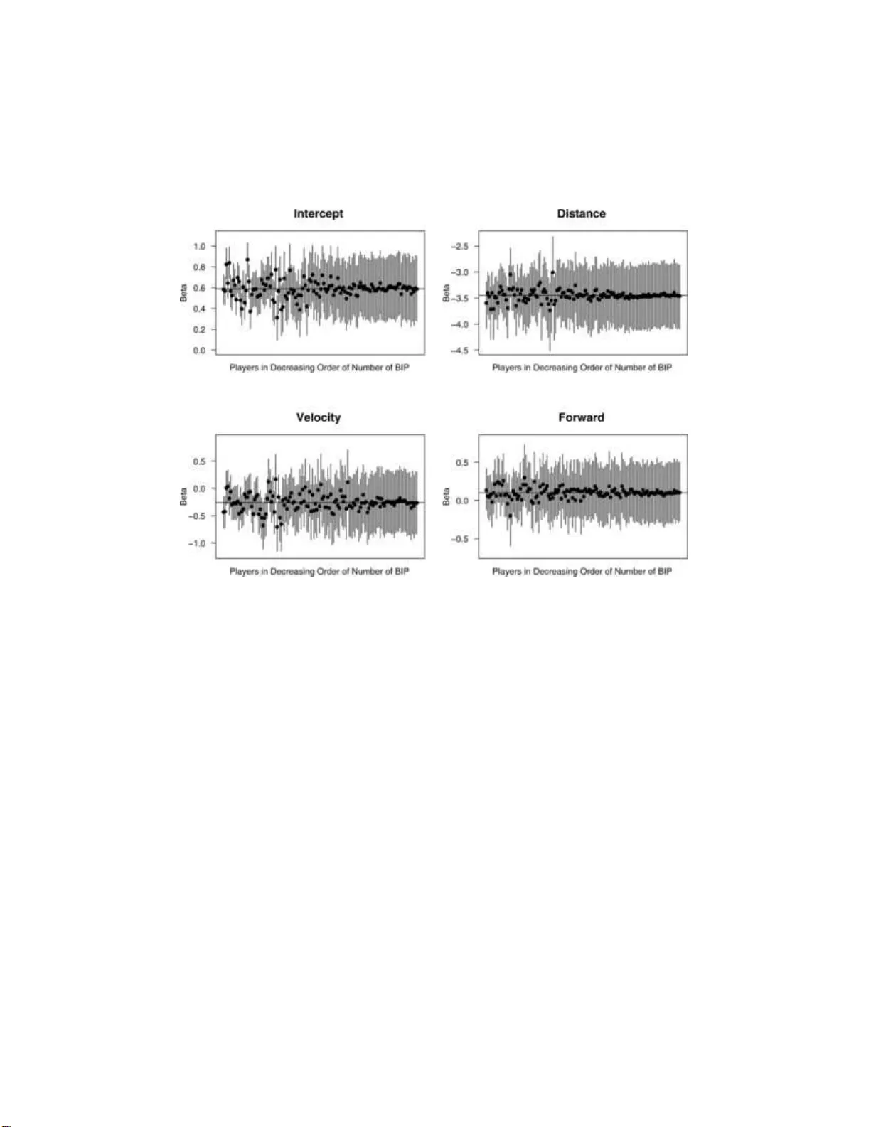
The Annals of Applie d Statistics 2009, V ol. 3, No. 2, 491–52 0 DOI: 10.1214 /08-A OAS228 c  Institute of Mathematical Statistics , 2009 BA YESBAL L: A BA YESIAN HIERAR CHICAL MODEL F OR EV ALUA TING FIELDING IN MAJOR LEA GUE BASEBALL By Shane T. Jensen, Kenne th E. Shirley and Abraham J. Wyner University of P ennsylvania The use of statistica l modeling in baseball has receiv ed substan- tial attention recently in b oth the media and academic communit y . W e focus on a rela tively under-explored topic: th e use of statisti- cal mod els for the analysis of fi elding based on high-resolution data consisting of on-field location of batted balls. W e combine spatial modeling with a hierarc hical Bay esian structure in order to ev aluate the p erformance of individual fielders while sharing information b e- tw een fielders at eac h position. W e present results across four s easons of MLB data (2002–2 005) and compare our approac h to other fielding ev aluation pro cedures. 1. In tro duction. Man y asp ects of ma jor league baseball are relativ ely easy to ev aluate b ecause of the mostl y discrete nature of the game: there are a relat iv ely small n u m b er of p ossible outcomes for eac h hitting or pitc hing ev ent. In addition, it is easy to determine which pla y er is resp onsible for these outco mes. Complicati ng and c onfounding factors e xist—lik e ball parks and league—but these differences are either sm all or a v eraged out ov er the course of a season. A p la ye r’s fielding abilit y is more d ifficult to ev aluate, b ecause fi elding is a nond iscrete asp ect of the game, with play ers fi elding balls-in-pla y (BIPs) across the conti n uous pla yin g su rface. Each ball-i n-pla y is either successfully fielded by a defensiv e pla y er, lea ding to an out (or multi ple o uts) o n th e p la y , or t he b all-in-pla y is n ot su ccessfully fielded, resulting in a h it. An inh eren tly complicate d asp ect of fi elding analysis is assessing the blame for an u nsuc- cessful fielding play . Sp ecific unsuccessful fielding pla ys can b e deemed to b e an “error” b y the official scorer at eac h game. T hese assigned errors are easy to tabulate and can b e us ed as a rudimen tary measure for comparing pla yers. How ev er, errors are a s u b jectiv e measure [ Kalist and Sp urr ( 2006 )] Received May 2008; revised December 2008. Key wor ds and phr ases. Spatial mo dels, Bay esian shrink age, baseball fielding. This is a n electronic reprint of the o riginal ar ticle published by the Institute of Mathematica l Statistics in The Annals of Applie d Statistics , 2009, V ol. 3 , No. 2, 491 –520 . This reprint differs from the origina l in pagination and typog raphic detail. 1 2 S. T. JENSEN , K . E. SHIR LEY AND A. J. WYNER that only tell part of the story . Additionally , errors are only r eserv ed for pla ys wh ere a b all-in-pla y is obvio usly mishandled, with no corresp onding measure for rewarding play ers for a particularly w ell-handled fielding pla y . Most analysts agree that a more ob jectiv e measure of fieldin g abilit y is the range of the fielder, though this qualit y is hard to measure. If a batte d ball sneaks th r ough the left side of the infield, for example, it is v ery difficult to kno w if a faster or b etter p ositioned shortstop could hav e reasonably made the pla y . C onfounding factors such as th e sp eed and tra jectory of th e b atted ball and the qualit y and range of ad j acen t fielders ab ound. F ur thermore, b ecause of the large and cont in u ous pla ying surface, the ev aluation of fi elding in ma jor league baseball p r esen ts a greate r mo deling c hallenge than the ev aluation of offensive con tributions. Previous approac hes ha ve a ddressed t his problem by a vo iding con tinuous mo dels and instead discretizing the pla ying su rface. The Ultimate Zone Rating (UZR) is based on a division of the pla ying field int o 64 large zones, with fielders ev aluated b y ta bulating their succe ssful pla ys within eac h zone [ Lic htman ( 2 003 )]. The Probab ilistic Mo del of Range (PMR) divides the field in to 18 pie slices (ev ery 5 degrees) on either side of second base, with fi elders ev aluated by tabulating their successful pla y s within eac h slice [ Pin to ( 2006 )]. Another similar m etho d is the recen tly pub lished Plu s-Min us system [ Dew an ( 2006 )]. The weakness of these metho ds is th at eac h zone or slice is quite large, wh ich limits the exten t to which differences b et ween fielders are detectable, sin ce ev ery ball hit in to a zone is treated equally . Our metho dology addresses the con tin u ous p la ying surface b y mo deling the success of a fielder on a giv en BIP as a function of the lo cation of that BIP , where lo cation is measured as a c ontinuous v ariable. W e fit a hier- arc hical Ba y esian mo d el to ev aluate the s u ccess of eac h individu al fielder, while sharing information b et wee n fi elders at the same p osition. Hierarc hical Ba ye sian m o dels ha ve also r ecen tly b een used b y Reic h et al. ( 2006 ) to esti- mate the spatial distribu tion of basket ball shot chart data. Our ultimate goal is to pro du ce an ev aluation by estimating the num b er of runs that a giv en fielder sa ves or costs his team dur ing the season compared to the a v erage fielder at h is p osition. S ince th is qu an tity is not directly observe d, it cannot b e used as the outcome v ariable in a statistic al mod el. T herefore, our ev al- uation requires t wo steps. First, we mo del the binary v ariable of wh ether a pla yer successfully fields a given BIP (an outcome w e can obs erve) as a func- tion of the BIP lo cation. Th en, we in tegrate o ver the estimated distribution of BIP lo cations and m u ltiply b y the estimate d consequence of a successful or unsuccessful pla y , measured in r u ns, to arriv e at our fi nal estimate of the n um b er of r u ns sav ed or cost by a giv en fielder in a season. W e present our Ba y esian hierarc hical m o del implemen ted on high-resolution data in Section 2 . In S ection 3 we illustrate our metho d u s in g one partic- ular p osition and BIP t yp e as an example. In Section 4 we describ e the BA YESI A N MOD ELING OF FI ELD I NG IN BASEBALL 3 Fig. 1. Contour plots of estimate d 2-dimensional densities of the 3 BIP typ es, using al l data fr om 2002–2005 . Note that the origin is lo c ate d at home plate, and the four b ases ar e dr awn into the plots as black dots, wher e the diagonal lines ar e the l eft and right foul lines. The outfield fenc e is not dr awn into the plot, b e c ause the data c ome fr om multiple b al lp arks, e ach wi th its outfield fenc e i n a differ ent plac e. The units of me asur ement for b oth axes ar e fe et. calculati ons w e make to conv ert the p arameter estimates fr om th e Ba y esian hierarc hical mo del to an estimate of the runs sav ed or cost. In Section 5 w e present our integ rated r esults, and we compare our r esu lts to those from a representa tiv e p revious metho d, UZR, in Section 6 . W e conclude with a discussion in Section 7 . 2. Ba ye sian hierarc hical mo del for individual pla y ers. 2.1. The data. Our fielding ev aluation is based up on high-resolution data collec ted by Baseball In fo Solutions [ BIS ( 2007 )]. Eve ry b all put in to pla y in a ma j or league baseball game is m app ed to an ( x, y ) co ordinate on the pla ying field, up to a resolution of approxima tely 4 × 4 feet. Our researc h team collect ed samples f r om sev eral companies that pr o vide high-resolution 4 S. T. JENSEN , K . E. SHIR LEY AND A. J. WYNER T able 1 Summary of mo dels BIP-ty p e Flyballs Liners Grounders P osition 1B 1B 1B 2B 2B 2B 3B 3B 3B SS SS SS LF LF CF CF RF RF data and after wa tc hing repla ys of sev eral games, we decided to u se the BIS data since it app eared to b e the most accurate. W e hav e four seasons of data (2002 –2005) , with around 120,00 0 balls-in-pla y (BIP) p er y ear. These BIPs are classified in to three distinct typ es: flyb alls (33% of BIP), liners (25% of BIP) and groun ders (42% of BIP). T h e flyballs catego ry also includes infield and outfield p op-ups. Figure 1 displa ys the estimated 2-dimensional densit y of eac h of the thr ee BIP types, plotted on the 2-dimensional pla ying surface. The areas of the field w ith the highest densit y of balls-in-pla y are indicated b y th e cont our lines whic h are in closest pro ximit y to eac h other. Not sur p risingly , the high-densit y BIP areas are quite d ifferen t b et ween the three BIP t yp es. F or flyb alls and liners, the lo cation of eac h BIP is the ( x, y )- co ord inate where the ball w as either caugh t (if it wa s caugh t) or where the ball landed (if it was not caugh t). F or ground ers, the ( x, y ) -lo cation of the BIP is set to the lo cation where t he g rounder w as fielded, either b y an infielder or an outfielder (if the ball made it through the infield for a h it). 2.2. Overview of our mo dels. The fir s t goa l of our analysis is to p roba- bilisticall y mo del the bin ary outcome of wh ether a fielder m ade a “successful pla y” on a ball batted into fair territory . W e fit a sep arate mod el f or eac h com bination of ye ar (2002– 2005), BIP type (flyball, liner, grounder) and p o- sition. T able 1 con tains a listing of the mo d els w e fit classified by p osition and BIP t yp e. Pitchers and catc hers we re excluded du e to a lac k of data. Also note that fly balls and liners are mo deled for all sev en remaining p o- sitions, whereas grounders are only mo d eled f or the infield p ositions. T h is giv es u s eigh teen mo dels to b e fit within eac h of the four yea rs, giving us 18 × 4 = 72 total mo del fits. The in puts a v ailable for mo deling include the iden tit y of the fielder pla ying the giv en p osition, the lo cation of the b atted ball, and the approxi mate v elo cit y of the batted ball, measured as an ordi- nal v ariable with three lev els (the v elo cit y v ariable is estimated by human observ ation of video, n ot using an y mac hinery). F or flyb alls and liners, a successful play is defined to b e a pla y in whic h the fi elder catc hes the ball in BA YESI A N MOD ELING OF FI ELD I NG IN BASEBALL 5 the air b efore it hits the ground. F or grounders, a su ccessful pla y is defined to b e a play in whic h the fi elder fields the grounder and r ecords at least one out on the play . Grounders and Flyballs/Liner BIPs are fundamen tally differen t in the wa y their lo cation data is recorded, as outlined b elo w, wh ic h affects our mo deling app r oac h. 1. Flyb al ls and liners : F or flyb alls and liners, the ( x, y )-lo cation of the BIP is set to the lo cation where the ball was either caugh t (if it w as caught ) or where the ball landed (if it w as not caugh t). W e mo d el the p rob ability of a catc h as a function of the distance a pla y er h ad to trav el to reac h the BIP lo cation, the direction he had to trav el (forw ard or bac kwa rd) and the v elo cit y of the BIP . Ou r flyball/liner distances must in corp orate t wo d imensions since a fielder tra v els across a t w o-dimensional plane (the pla ying fi eld) to catc h the BIP . 2. Gr ounders : F or ground ers, the ( x, y )-lo cation of the BIP is set to the lo cation where the groun der was fielded, either by an infi elder or an out- fielder (if the b all made it through the infield for a h it). As we did w ith flyballs/liners, we mo del th e pr obabilit y of an infi elder successfully field- ing a grounder as a function of the d istance, direction and v elocit y of the grounder. F or grounders, how ev er, distance is measured as the angle, in degrees, b et ween the tra jectory of the groundball from h ome plate and the (imag inary) line drawn b et ween the in fielder’s starting location and home p late, with direction b eing fact ored in b y allo win g differen t proba- bilities for fielders mo ving the same num b er of degrees to the left or the righ t. T he grounder distance only m ust incorp orate one dimension since the infielder trav els along a one-dimensional path (arc) in order to field a grounder BIP . Figure 2 giv es a graph ical representa tion of the difference in our approac h b et w een grounders a nd fl ys/liners. It is worth noting, h o wev er, that the distance (for flyballs/liners) or angl e (for grounders) tha t a fielder must tra vel in order to reac h a BIP is act ually an e stimated v alue, since the actual starting location of th e fielder for any particular p la y is not included in the data. In stead, the starting lo cation for eac h p osition is estimated as the lo cation in the field where eac h p osition has the h ighest ov erall prop ortion of successful plays. The distance/angle trav eled for eac h BIP is then calculated relativ e to this estimat ed starting p osition f or eac h pla ye r. 2.3. Mo del for flyb al ls/liners using a two-dimensional sp atial r e pr esenta- tion. W e p resen t our m o del b elo w in the con text of flyballs (whic h also include infield pop-up s), b u t the same metho dology is used f or li ners as w ell. F or a particular fielder i , w e denote the num b er of BIPs hit while that pla yer w as p la ying defense n i . The outcome of eac h pla y is either a success 6 S. T. JENSEN , K . E. SHIR LEY AND A. J. WYNER Fig. 2. Two-dimensional r epr esentation for flyb al ls and liners vers us one-dimensional r epr esentation for gr ounders. or failure: S ij =  1 , if th e j th flyb all hit to the i th pla yer is caught , 0 , if th e j th flyb all hit to the i th pla yer is not caugh t. These observ ed su ccesses and f ailures are mo deled as Bernoulli realiz ations from an un d erlying even t-sp ecific probabilit y: S ij ∼ Bernoulli( p ij ) . (1) As mentioned ab o ve , the a v ailable co v ariates are the ( x, y ) location and the vel o cit y V ij of the B IP . Although the v elocit y is an ordin al v ariable V ij = { 1 , 2 , 3 } , we treat v elo city as a con tin u ous v ariable in our mo del in order to redu ce the num b er of co efficien ts included. T he Bernoulli probabilities p ij are mod eled as a fun ction of distance D ij tra vel ed to the BIP , v elo cit y V ij and an indicator for the d irection F ij the fielder has to mo ve to ward the BIP ( F ij = 1 for moving forward, F ij = 0 for mo ving bac kward): p ij = Φ( β i 0 + β i 1 D ij + β i 2 D ij F ij + β i 3 D ij V ij + β i 4 D ij V ij F ij ) (2) = Φ( X ij · β i ) , where Φ( · ) is the cum ulativ e distribu tion function for the Normal distribu- tion and X ij is a v ector of the co v ariate terms in equation ( 2 ). Note that the cov ariates D ij and F ij are themselve s functions of the ( x, y ) co ordinates for that particular BIP . This mo del is recognizable as a p r obit regression mo del with in teractions b et ween co v ariates that allo w for d ifferen t proba- bilities f or mo ving the same d istance in the forward direction v ers u s the bac kward d irection. W e can giv e natural in terpretations to the parameters of this fly/liner probit mo del. Th e β i 0 parameter con trols the probabilit y BA YESI A N MOD ELING OF FI ELD I NG IN BASEBALL 7 of a catc h on a fly/liner h it directly at a fi elder ( D ij = 0). The β i 1 and β i 2 parameters cont rol the range of th e fielder, m o ving either bac kw ard ( β i 1 ) or forw ard ( β i 2 ) to w ard a fly/liner. T he p arameters β i 3 and β i 4 adjust the probabilit y of success as a fun ction of v elo cit y . 2.4. Mo del for gr ounders using a one-dimensiona l sp atial r e pr esentation. The outco me of eac h grounder BIP is either a success or failure: S ij =  1 , if th e j th grounder hit to the i th play er is fielded su ccessfully , 0 , if th e j th grounder hit to the i th play er is not fi elded s uccessfully . Grounders ha v e a similar observed data lev el to their mo del, S ij ∼ Bernoulli( p ij ) , (3) except that the und erlying pr obabilities p ij are mo deled as a fun ction of angle θ ij b et w een the fielder and the BIP lo cation, the v elo cit y V ij of the BIP , and an indicator for the direction L ij the fielder has to mo ve to wa rd the BIP ( L ij = 1 for moving to the left, L ij = 0 for moving to the righ t): p ij = Φ( β i 0 + β i 1 θ ij + β i 2 θ ij L ij + β i 3 θ ij V ij + β i 4 θ ij V ij L ij ) (4) = Φ( X ij · β i ) . Again Φ( · ) represen ts the cum ulativ e d istribution function for the Normal distribution and X ij is a v ector of the co v ariate terms in equation ( 4 ). W e can also giv e natural inte rpretations of the parameters in this grounder probit mo del. The β i 0 parameter cont rols the probabilit y of a catc h on a grounder hit directly at the fielder ( D ij = 0). The β i 1 and β i 2 parameters contro l the range of the fielder, movi ng either to the righ t ( β i 1 ) or to the left ( β i 2 ) to ward a groun d er. The parameters β i 3 and β i 4 adjust the probabilit y of success as a function of ve lo cit y . 2.5. Shar ing information b e twe en players. W e can calculate parameter estimates β i for eac h pla y er i separately using standard p robit regression soft ware. Ho wev er, we will see in S ection 3.2 b elo w that these parameter esti- mates β i can b e h ighly v ariable for play ers with small sample sizes (i.e., those pla yers who f aced a small n umber of BIPs in a giv en y ear). Th is problem can b e addressed by using a hierarchica l mo del w here eac h set of pla y er-sp ecific co efficients β i are mo deled as sharing a common prior d istribution. This hi- erarc hical structure allo w s for information to b e shared b et wee n all pla y ers at a p osition, wh ic h is esp ecially imp ortan t for pla yers with smaller num b ers of opp ortunities. Sp ecifically , w e mo del eac h pla y er-sp ecific co efficien t as a dra w from a common distribution sh ared by all pla y ers at a p ositio n: β i ∼ Normal( µ , Σ) , (5) 8 S. T. JENSEN , K . E. SHIR LEY AND A. J. WYNER where µ is the 5 × 1 ve ctor of means and Σ is the 5 × 5 prior co v ariance matrix shared across all pla yers. W e assume a p riori indep end ence of the comp onen ts of β i , s o that Σ has off-diagonal elemen ts of zero, and diago nal elemen ts of σ 2 k ( k = 0 , . . . , 4). Although the comp onents of β i are assumed to b e indep en d en t a priori, there will b e p osterior d ep endence b et w een th ese comp onen ts ind uced b y the data. Th e functional form of this p osterior d e- p endence is giv en in our supplemen tary materia ls section on mo del imple- men tatio n [ Jensen, Shirley and Wyner ( 2009 )]. Finally , we must also sp ecify a p rior distribution for the shared pla y er parameters ( µ k , σ k : k = 0 , . . . , 4), whic h w e c ho ose to b e noninformativ e f ollo wing t he recommendation of Gelman ( 20 06 ), p ( µ k , σ k ) ∝ 1 , k = 0 , . . . , 4 . (6) W e also explored the use of alternativ e prior sp ecifications, including a prop er inv erse-Gamma p rior distribution f or σ 2 k : ( σ 2 k ) − 1 ∼ Gamma( a, b ), where a and b are small v alues ( a = b = 0 . 00 01). W e observe d v ery little d ifference in our p osterior estimat es using this alternativ e prior distribu tion. F or eac h p osition and BIP t yp e, our full set of unkno w n parameters are β , the N × 5 matrix con taining the co efficien ts of eac h play er at a particular p osition ( N = num b er of p la ye rs at that p osition), as w ell as µ , the 5 × 1 v ector of coefficient means, and σ 2 , the 5 × 1 v ector of coefficient v ariances shared b y all pla y ers at that p osition. F or eac h p osition and BIP-type, w e separately estimate the p osterior distribu tion of our parameters β , µ and σ 2 , p ( β , µ , σ 2 | S , X ) ∝ p ( S | β , X ) · p ( β | µ , σ 2 ) · p ( µ , σ 2 ) , (7) where S is the collection of all outcomes S ij and X is a collection of all lo- cation and v elocity co v ariates X ij . W e estimate the p osterior d istribution of all unknown parameters at eac h p osition and BIP-t yp e u sing MCMC meth- o ds. Sp ecifically , we emp lo y a Gibbs sampling strategy [ Geman and Geman ( 1984 )] that builds up on standard hierarc h ical regression methodology [ Gelman et al. ( 2003 )] and data augmenta tion for p robit mo dels [ Alb ert and Ch ib ( 1993 )]. Additional details are pr o vided in our sup plemen- tary materials [ Jensen, Shirley and Wyner ( 2009 )]. Ou r estimati on pro ce- dure is rep eated for eac h of the eight een com binations of p osition and BIP t yp e listed in T able 1 , and for eac h of the 4 y ears from 2002–20 05, for a grand total of 18 × 4 = 72 fitted mo dels. In the n ext section w e provide a detailed examination of our mo d el fi t f or a particular p osition, BIP-type and y ear: fl yballs fi elded by cent erfielders in 200 5. 3. Illustrati on of our mo d el: fl yballs to CF in 2005. Of the 38,000 flyballs that we re h it into fair territory in 2005 , ab out 11,000 of them we re caught BA YESI A N MOD ELING OF FI ELD I NG IN BASEBALL 9 Fig. 3. Plot of 5062 flyb al ls c aught by c enter fielder (left), and 10,705 flyb al ls not c aught by CF or any other fielder (right). T o gether these 15,767 p oints c omprise the set of CF-el- igible flyb al ls f r om 2005. However, only flyb al ls that fal l within 250 f e et of the CF lo c ation ar e use d in our mo del fit, though this r estriction only excludes a few flyb al ls lo c ate d ne ar home plate. b y the CF. Of the 27,000 that w ere n ot caugh t by the C F, ab out 22,00 0 were caugh t b y one of the other eight fielders and ab out 5000 w ere n ot caugh t b y an y fielder. The 22,000 flyballs caugh t by one of the other eig h t fielders are not treate d as failures for the CF since it is unkno wn if the CF w ould ha v e caugh t them had the other fielder not made the catc h. Th ese observ ations are treated as missing data with r esp ect to mod eling the fielding abilit y of the CF. The “CF-eligi ble” fl yballs in 2005 are all flyballs that we re either (1) caugh t by the CF or (2) not caugh t b y any other fielder. T here w ere exactly 15,767 CF-eligible flyballs in 2005. Figure 3 con tains plots of the CF-eligible flyballs that w ere caugh t by the CF (left), and those that were not caugh t by the CF (right) . In the righ t plot, data are s parse in the regions where the left fielder (LF) and right fielder (RF) pla y , as well as in the infi eld. Most of the flyballs hit to these lo cations we re caugh t by the LF, RF or an infielder, and are therefore not includ ed as CF-eligible flyballs. Additionally , we restrict ourselv es only to flyballs that landed within 250 feet of the CF lo cation for our mo del estimation, s ince tra veli ng an y larger d istance to mak e a catc h is unrealistic. 3.1. Data and mo del for il lustr ation. F or eac h flyball, the data consist of the ( x, y )-co ordinates of the flyball lo cation, the iden tit y of the CF pla ying defense, and the v elo cit y of th e flyball, whic h is an ordinal v ariable with 3 lev els, where 3 indicates the h ardest-hit b all. In 2005 there were N = 138 unique CFs that pla y ed defense for at le ast one CF-eligible flyball. Th e 10 S. T. JENSEN , K . E. SHIR LEY AND A. J. WYNER n um b er of fl yballs p er fi elder, n i , r anges from 1 to 531, and its distribution is ske w ed to the r igh t. W e denote the ( x, y )-co ordinate of the j th flyball hit to the i th CF as ( x ij , y ij ). Based on the ov erall distribu tion of these fl yballs, w e estimate the id eal starting p osition of a CF as the co ordinate in the field with th e highest catc h pr obabilit y across all CFs. Th is co ordinate, whic h w e call the C F cen troid, w as estimated to b e (0 , 324), which is 324 feet in to cen terfield straigh t from home plate. F or the j th ball hit to the i th CF, we ha ve the follo wing co v ariates for our mo del fit: the distance from the flyball lo cation to the CF cen troid, D ij = q ( x ij − 0) 2 + ( y ij − 324) 2 , and the v elo cit y of the flyball V ij whic h tak es on an ordinal v alue from 1 to 3 . As men tioned ab o ve, our mo d el estimatio n only considers flyballs wh ere D ij ≤ 250 feet. W e also create an indicator v ariable for whether the flyb all was h it to a lo cation in fron t of the C F: F ij = I ( y ij < 324). F ij = 1 corresp onds to fl yballs where the CF m u st mov e forward, whereas F ij = 0 corresp onds to flyballs where th e CF m u st mo v e bac kward. F or the purp ose of this illustration only , we consider a simplified v ersion of our mo del that do es n ot ha ve interac tions b et w een these co v ariates. Sp ecifically , we fi t the follo wing simplified mo del: P ( S ij = 1) = Φ( β i 0 + β i 1 D ij + β i 2 V ij + β i 3 F ij ) (8) = Φ( X ij · β i ) , where Φ ( · ) is the cum u lativ e distribu tion function for th e standard normal distribution. In our full analysis, w e fi t the mo d el with inte ractions from equation ( 2 ) in Section 2.3 . F or this illustration only , w e also rescale the predictors D ij , V ij and F ij to hav e a mean of zero and an sd of 0.5, so that the p osterior estimates of β are on roughly the same scale, and to reduce the correlat ion b etw een the in tercept and the slop e co efficien ts. 3.2. Mo del implementation for il lustr ation. W e use the Gibbs sampling approac h outlined in our su pplemen tary materials [ Jensen, Shirley and Wyner ( 2009 )] to fit our simplified mod el ( 8 ) for CF flyballs in 2005. Figure 4 dis- pla ys p osterior means and 95% p osterior interv als for the four elemen ts of the co efficient mean ve ctor µ shared across all CFs. As exp ected, the co effi- cien ts for distance and v elo cit y are n egativ e and, not sur prisingly , distance is clearly the predictor that exp lains th e most v ariation in the outcome. The co efficient for forwa rd is p ositiv e, whic h means that it is easier for a CF to catc h a flyball hit in front of h im than b ehind him for the same distance and velocit y . The in tercept is p ositiv e, and is ab out 0.5 8. The in tercept can b e in terpreted as the in v erse probit p robabilit y [Φ(0 . 58) ≈ 72%] of cat c h in g a flyball hit to the mean distance from the CF (ab out 90 feet) at the mean v elo cit y (ab out 2.2 on the scale 1–3). Figure 5 displa ys three differen t estimate s of β : BA YESI A N MOD ELING OF FI ELD I NG IN BASEBALL 11 Fig. 4. Posterior me ans and 95% intervals for the p opulation-level slop e c o efficients µ . 1. no p o oling: β estimates fr om mo del with no common d istribution b etw een pla yer coefficien ts, 2. complet e p o oling: β estimate s from mo del with all p la ye rs com bin ed to- gether for a single set of co efficien ts, 3. partial p o oling: β estimates from our mo del describ ed ab o ve , with s ep a- rate pla yer co efficien ts that share a common distribution. F rom Figure 5 it is clear there that there wa s substant ial shrink age for the Distance and F orward co efficien ts, sligh tly less shrin k age for the V elo cit y co efficient, and not muc h shrink age for the interce pt. Th e p osterior means for σ k w ere 0.15, 0.28, 0.28 and 0.17 for the In tercept, Distance, V elocity and F orward co efficien ts, resp ectiv ely . The p osterior distributions of σ k did not in clude any mass near zero, in d icating that complete p o oling is also not a go o d mo del, sin ce these estimates should app roac h zero if there is not sufficien t evidence of heterogeneit y among individu al pla yers. Figure 6 includes all N = 138 estimates of β i ( i = 1 , . . . , N ) with 95% in terv als included. The estimates a re d ispla yed in decrea sing ord er of n i from left to righ t, where the pla y er w ith the most BIP observ ations had n 1 = 531 observ ations, and six pla ye rs had just 1 observ ation. The pla ye rs with few er observ ations had their estimates shrun k muc h closer to the p opulation means display ed in Figure 4 , wh ich are also dr a wn as horizon tal lines in Figure 6 , and they also had larger 95% in terv als, as one w ould exp ect with few er observ ations. On e in teresting thing to note is that a small n u m b er of pla yers ha v e estimate d v elo cit y coefficien ts that are p ositiv e, meaning they are relativ ely b etter at catc hing flyballs that are h it faster, and at least one pla yer has a forward co efficient that is negativ e, meaning he is b etter at catc hing balls hit b ehind h im. T o chec k the fit of the mo d el graph ically , we examine a num b er of residual plots, as sh o wn in Figure 7 . Figure 7 (a) shows the h istogram of the residuals, r ij = y ij − Φ( X ij ˆ β i ) , 12 S. T. JENSEN , K . E. SHIR LEY AND A. J. WYNER Fig. 5. Thr e e differ ent estimates of β , c orr esp onding to no p o oling, p artial p o oling and c omplete p o oling. Only the 45 CFs with the lar gest sample sizes ar e include d in these plots, b e c ause the no-p o oling estimates for many of the CFs wi th li ttle data wer e undefine d, did not c onver ge or wer e cle arly unr e alistic. for the j th flyball hit t o the i th pla y er, where ˆ β i is the p osterior mean v ector of the r egression co efficien ts for pla y er i . The long left tail in the Figure 7 (a) histogram consists of flyballs that should ha ve b een caugh t (i.e., had a high predicted pr obabilit y of b eing caugh t) bu t were not caugh t. Bins of residuals were constructed by ordering the residuals r ij in terms of the predicted p robabilit y o f a catc h Φ( X ij ˆ β i ) and th en d ividing the ordered residuals in to equal sized bins (ab out 150 r esiduals p er bin). Th e a v erage of all residuals within eac h bin was calculated, w hic h w e call the a verag e binned residuals. These a verag e binned residuals are plotted as a fu n ction of predicted probabilities, whic h are the blac k p oin ts in Figure 7 (b). A go o d mo del w ould sho w no obvious p attern in these a verage binned residuals (blac k dots). I t app ears that our mo del slightly o verestima tes the p robabilit y of catc hing the ball for predicted probabilities b et ween 0% and 20%, and sligh tly underestimates the probabilit y of c atc hing the ball for predicte d probabilities b et wee n 30% and 60%. BA YESI A N MOD ELING OF FI ELD I NG IN BASEBALL 13 Fig. 6. Posterior me ans and 95% p osterior intervals f or c o efficients f or al l N = 138 individual players. In e ach plot, the distribution of β ij for e ach player i i s r epr esente d by a cir cle at the p osterior me an and a vertic al li ne for the 95% p osterior interval. The players ar e displaye d in de cr e asing or der of n i fr om left to right, with the first player having the lar gest numb er of BIP observations ( n 1 = 531 ) and the l ast player having the smal lest numb er of BIP observations n 138 = 1 . In order to pro vide additional con text to the observ ed r esiduals, w e also constructed a verag e binn ed residu als from 500 p osterior p r ed ictiv e sim ula- tions of new data. These p osterior pr edictiv e a verag e binn ed residuals are sho w n as gra y p oin ts in the backg round of Figure 7 (b). W e also constructed 95% p osterior in terv als for the a verag e binned residu als b ased up on these p osterior predictiv e simulati ons, and t hese int erv als are ind icated by th e blac k lines in Fig ure 7 (b). W e see that the p attern of our observ ed a v erage binned residuals is not unusual in the conte xt of their p osterior predictiv e distribution. In fact, w e find that exactly 95 out of 100 of our observe d a v- erage binned residu als f all w ithin their 95% p osterior predictiv e in terv als, whic h suggests a reaso nable fit. Figure 7 (c) pr o vides a d ifferen t view of this same go o dn ess-of-fit c hec k by plotting the actual binn ed probabilities against the b inned probabilities pr edicted b y the m o del. Just as in Figure 7 (b), the blac k p oints indicate the relationship from our actual d ata, whereas the gra y p oint s come from the same 500 p osterior p redictiv e simulat ions. W e see that 14 S. T. JENSEN , K . E. SHIR LEY AND A. J. WYNER Fig. 7. Plot (a) on the left shows the histo gr am of the fitte d r esiduals, define d as the differ enc e b etwe en the outc ome and the exp e cte d outc ome as estimate d fr om the mo del us- ing p osterior me ans. Plot (b) plots aver age binne d r esiduals against pr e di cte d pr ob abilities, wher e the aver age binne d r esiduals ar e the aver age of r esiduals that wer e binne d after b eing or der e d by the pr e dicte d pr ob abilities. Black dots ar e the actual aver age binne d r esiduals fr om our data. T he gr ay p oints in the b ackgr ound ar e aver age binne d r esiduals fr om 500 p osterior pr e di ctive simulations. The black lines r epr esent the b oundaries of 95% inter- vals for the aver age binne d r esiduals fr om our p osterior pr e dictive simulations. The lack of smo othness in the interval b oundaries i s due to r andomness in our p osterior pr e di c- tive simulations. Plot (c) is c onstruc te d the same way as plot (b ) , exc ept that the y-axis c orr esp onds to the bi nne d pr ob abili ties r ather than binne d r esiduals. the actual b in ned probabilities lie approxi mately along the 45-degree line of equalit y wh en plotted against the predicted binned p robabilities. W e also examined the association b et ween our residuals and individual co v ariates: distance, v elo cit y , and direction, as sh o wn in Figure 8 . The p lots in Figure 8 revea l no ob vious patterns in the r esiduals with resp ect to the individual co v ariates, except p ossib ly a sligh t ov erestimatio n of the p roba- BA YESI A N MOD ELING OF FI ELD I NG IN BASEBALL 15 Fig. 8. Plot (a) c ontains aver age binne d r esiduals plotte d vs. distanc e. Plot (b) is a b oxplot of i ndividual r esiduals r ij gr oup e d by the thr e e differ ent levels of velo city. Plot (c) is a b oxplot of individual r esiduals r ij gr oup e d by the di r e ction indi c ator: moving forwar ds or b ackwar d. bilit y of a catc h f or flyballs hit at a distance of 150 –200 feet from the CF. This o verestima tion, ho w ever, app ears to b e on the order of 1–2%, whic h is small relativ e to the n atur al v ariabilit y in pred ictions for flyballs hit at shorter distances. W e examined the shrink age of the enti re set of fi tted p robabilit y curv es for the whole p opulation of CFs, sho wn in Figure 9 . In this figure, we plot the fitted p r obabilit y curv es for all CFs (with fi xed velocit y v = 2 and for- w ard = 1) from th r ee d ifferen t metho ds. Plot (a) giv es the fitted probabilit y curv es estimated with no p o oling—they are the curv es calcula ted using the parameter estimates from the top h orizon tal line in Figure 5 . S ev eral of these curv es are extreme in shap e, with the most v ariable curv es coming from pla y- ers w ith littl e observ ed d ata. Plot (b ) giv es the curve s based on parameter estimates using th e probit mo del with our h ierarc hical extension presen ted in Section 2.5 —the estimates from the “partia l-p o oling” middle line in Fig - 16 S. T. JENSEN , K . E. SHIR LEY AND A. J. WYNER Fig. 9. The fitte d pr ob ability curves for e ach 2005 CF as a f unction of distanc e for flyb al ls hit at fixe d velo city v = 2 in the forwar d dir e ction. Plot (a) has curves estimate d with no p o oling. Plot (b) has the curves estimate d by p artial p o oli ng via our hier ar chic al mo del (using p osterior me ans for indivi dual players). Plot (c) is the p opulation m e an curve, estimate d with c om pl ete p o oling. ure 5 . W e see the stabilizing shrink age of the partial p o oling curv es to ward the aggregate m o del estimated using all data across p lay ers, which is dra wn in p lot (c) of Figure 9 . It should b e noted that the partial p o oling curves BA YESI A N MOD ELING OF FI ELD I NG IN BASEBALL 17 are estimated usin g p osterior means from the hierarc hical mo d el. W e also explored th e use of a logit mo del f or this d ata, and found the mo del fit wa s similar to the probit mo d el, whic h we pr eferred b ecause of its compu tational con venie nce. In addition to th ese o verall ev aluations, we also p erformed a range of p osterior predictiv e c hec ks for the fielding abilitie s of individual CFs. It is of interest to see if the mo del is accurately describing the het erogeneit y b et w een CFs, so w e examined th e d ifference in the p ercen tage of flyballs caugh t b etw een the b est C F ve rsus the worst CF. W e simulate d 500 p osterior predictiv e datasets from tw o d ifferen t mo dels: (a) our full hierarc h ical mo d el with partial p o oling and ( b) t he complete po oling m o del where a sin gle set of co efficien ts is fit to the data p o oled across all CFs. F or eac h of our p osterior predictiv e datasets, we calculate d the difference in the p ercentag e of flyballs caugh t b et wee n the b est and wo rst CF among the 15 CFs with the most opp ortunities. Figure 10 shows the d ensit y of the d ifference in the p ercen tage of flyballs caugh t b et w een the b est and w orst CF for the partial p o oling mo del (solid densit y line) and the complete p o oling m o del (dashed Fig. 10. The p osterior pr e dictive density of the differ enc e in the p er c entage of flyb al ls c aught b etwe en the b est CF versus the worst CF for two mo dels. The solid-line d density r epr esents the p artial p o oling mo del and the dott e d-line d density r epr esents the c omplete p o oling mo del. These densities wer e estimate d using 500 datasets simulate d fr om p osterior pr e dictive distribution under these two mo dels. The vertic al li ne r epr esents the di ffer enc e b etwe en b est and worst CF fr om our observe d data. 18 S. T. JENSEN , K . E. SHIR LEY AND A. J. WYNER densit y line). The difference b et w een b est and w orst CF from our observed data ( 15 . 1% = 74 . 1% for Andr u w Jones − 59.0% fo r Presto n Wilson) is sho w n as a vertic al line. W e see that th e actual difference from our observ ed data is m uc h more like ly und er the partial p o oling mo del th an the complete p o oling mo del. Not su rprisingly , the complete p o oling m o del underestimates the heterogeneit y among p la ye rs. Und er partial p o oling, how ev er, add itional v ariabilit y is incorp orated via the h ierarc hical mo del, so that the co efficien ts for eac h pla yer are different , and greater differences in abilit y are allo w ed. One add itional concern ab out our mod el is the p oten tial effect of outliers on the estimation of fitted pr ob ability curve s. W e explored the effect of a sp e- cific type of outlier: plays that w ere scored as fielding errors. Fielding errors are failures on BIPs that sh ould hav e b een fielded su ccessfully , as judged by the official scorer for the game. Although errors con tain defensiv e informa- tion and w e prefer their inclusion in our mo d el, the influ ence of these errors could b e sub stan tial s in ce they are, b y definition, unexp ected resu lts r elativ e to the fi elders’ abilit y . W e ev aluated this infl uence on our inference for CFs b y r e-estimati ng our fitted probabilit y models on a dataset with all fi elding errors remov ed. These r e-estimat ed prob ability curv es fr om our Ba y esian hierarc hical mo del w ere essen tially iden tical to the curves estimated with the errors included i n our dataset. Ho w ever, t he probabilit y cur v es esti- mated without any p o oling of information w ere muc h more sensitive to the inclusion/exclusion of errors. The sharing of information b et w een play ers through our h ierarc hical mo d el seems to con trib u te additional robustness to wa rd outlying v alues (in the form of err ors). 4. Con ve rting mo del estimates to runs sav ed or cost. In this section w e use the fitted pla yer-specific probabilit y mo dels from ( 2 ) and ( 4 ) for eac h BIP t yp e and season to estimate the n um b er of runs that eac h fi elder would sa ve or cost his team ov er a fu ll season’s wo rth of BIPs, compared to the a vera ge fielder at his p osition for that y ear. 4.1. Comp arison to aggr e gate curve at e ach p osition. Our pla y er-sp ecific co efficients β i can b e u sed to calculate a fitted probabilit y curv e f or eac h individual play er as a f u nction of lo cation and ve lo cit y . F or flyb alls and liners, the individual fitted probabilit y curve is denoted p i ( x, y , v ) , the estimated probabilit y of catc hing a flyball/liner hit to lo cation ( x , y ) a t v elocity v . F or grounders, the individual fitted pr obabilit y curv e is denoted p i ( θ , v ), the probabilit y of successfully fielding a grounder hit at angle θ at velocit y v . Our Gibbs sampling implement ation giv es us the full p osterior d istribution of our play er-sp ecific coefficien ts β i , whic h w e can use to calculate the full p osterior distrib ution of our fitted probabilit y curv es p i ( x, y , v ) or p i ( θ , v ). Alternativ ely , we can calculate the p osterior m eans ˆ β i for eac h β i v ector, BA YESI A N MOD ELING OF FI ELD I NG IN BASEBALL 19 and us e ˆ β i to fit a single probabilit y curv e ˆ p i ( x, y , v ) or ˆ p i ( θ , v ) f or eac h pla yer and BIP-t yp e. F or n o w, w e fo cus on these single fitted p robabilit y curv es, ˆ p i ( x, y , v ) or ˆ p i ( θ , v ), for eac h p la ye r. In Section 4.2 b elo w, w e will return to an approac h based on the full p osterior d istribution of eac h β i . With these p osterior mean fi tted curv es ˆ p i ( x, y , v ) or ˆ p i ( θ , v ), we can quan- tify the difference b et w een pla y ers b y comparing their individual probabil- ities of making an out relativ e to an a v erage p la ye r at th at p osition. The mo del f or the av erage pla y er can b e calculate d in sev eral differen t w a ys. A single probit r egression mo del can b e fit to the observe d data aggregat ed across all play ers at that p osition to calculate the maxim um lik eliho o d esti- mates ˆ β + , or we can use the p osterior mean of the p opu lation p arameters ˆ µ . These p opulation parameters ˆ β + can b e used to calculate a fitted curv e ˆ p + ( x, y , v ) or ˆ p + ( θ , v ) for the a v erage pla yer (for fly b alls/liners or groun ders, resp ectiv ely). Figure 11 illustrates the comparison on ground er curve s b e- t ween the a v erage m o del for the SS p osition and t w o individual fielders. F or eac h p ossible angle θ and v elo cit y v , we can calculate the difference [ ˆ p i ( θ , v ) − ˆ p + ( θ , v )] b etw een fielder i ’s probabilit y of success and the a v er- age probabilit y of success, wh ic h is the difference in h eigh t b et ween the individual’s curve and the a v erage curve, giv en in Figure 11 . A p ositiv e dif- ference at a p articular angle and v elocit y means that the individual pla yer is making a higher prop ortion of successful pla ys than the av erage fielder on balls hit to that angle at that vel o cit y . A negativ e difference means that the ind ividu al pla yer is making a lo w er prop ortion of successful pla ys than Fig. 11. Comp arison of the gr ounder curves of two i ndividual SSs ˆ p i ( θ , v ) to the aver age SS curve ˆ p + ( θ , v ) f or velo city fixe d at a mo der ate value of v = 2 . 20 S. T. JENSEN , K . E. SHIR LEY AND A. J. WYNER Fig. 12. Comp arison of CF curve ˆ p i ( x, y , v ) f or Jer emy R e e d with aver age CF curve ˆ p + ( x, y , v ) for flyb al l s with velo city v = 2 in 2005. Plot (a) shows the curves ˆ p i ( x, y , v ) vs. ˆ p + ( x, y , v ) as a function of di stanc e moving f orwar d fr om the CF lo c ation. Plot (b ) shows the curves ˆ p i ( x, y , v ) vs. ˆ p + ( x, y , v ) as a function of distanc e moving b ackwar d f r om the CF lo c ation. Plot (c) shows a 2-dimensional c ontour plot of [ ˆ p i ( x, y , v ) − ˆ p + ( x, y , v )] . R e e d’s pr ob ability of c atching a b al l i s r oughly the same as the aver age player at short distan c es, but is ab out 8% lar ger at a distanc e of ab out 100 fe et. Also , the differ enc e i n pr ob ability for R e e d vs. the aver age CF i s sli ghtly l ar ger for flyb al ls hit in the b ackwar d di r e ction than for those hit in the forwar d dir e ction. the a v erage fi elder on balls hit to that angle at that ve lo cit y . F or our fly- balls/liners mo dels, the calcula tion is s imilar, except that w e need to cal- culate these differences for all p oin ts around the fi elder lo cation in t wo d i- mensions. Figure 12 illustrates the comparison of probabilit y curves b et w een individual pla y ers and the a v erage curve for the CF p osition for fl yballs. F or eac h p ossible location ( x, y ) and v elo cit y v , w e can calculate the difference [ ˆ p i ( x, y , v ) − ˆ p + ( x, y , v )] b et w een fielder i ’s probability of success and the a v- erage p robabilit y of success, wh ic h is the difference b et wee n the t wo surfaces sho w n in Figure 12 . BA YESI A N MOD ELING OF FI ELD I NG IN BASEBALL 21 4.2. Weighte d aggr e gation of individual differ enc es. The fielding curv es ˆ p i ( x, y , v ) and ˆ p i ( θ , v ) for ind ividu al pla yers giv e us a graphical ev aluation of their relativ e fielding qu alit y . F or example, it is clear from Figure 11 that Adam Ev erett h as ab ov e av erage range for a s h ortstop, whereas Derek Jeter has b elo w a v erage range for a shortstop. Ho we v er, we are also in ter- ested in an o verall numerical ev aluation of eac h fielder whic h we will call “SAFE” for “Spatial Aggrega te Fielding Ev aluation.” F or flyballs or liners, one candidate v alue for eac h fielder i could b e to aggregate the individu al differences [ ˆ p i ( x, y , v ) − ˆ p + ( x, y , v )] o ve r all co ord inates ( x, y ) and ve lo cities v . F or ground ers, the corresp ondin g v alue would b e the aggrega tion of indi- vidual differences [ ˆ p i ( θ , v ) − ˆ p + ( θ , v )] o v er all angles θ and v elocities v . T hese aggrega tions could b e carried out b y numerical in tegratio n o ver a fine grid of v alues. Ho wev er, these simple inte grations d o not tak e in to accoun t the fact that some co ordinates ( x, y ) or angles θ ha ve a higher BIP fr equency during the course of a season. As we saw in Figure 1 , the spatial d istribution of BIPs ov er the p la ying field is extremel y non un iform . Let ˆ f ( x, y , v ) b e the k ern el densit y estimate of the frequency with which flyb alls/li ners are h it to co ordinate ( x, y ), whic h is estimate d sep arately f or eac h v elo cit y v . Let ˆ f ( θ, v ) b e the kernel densit y estimate of th e fr equency with which groun ders are hit to angle θ , wh ic h is estimated separately for eac h v elocit y v . Eac h fielder’s ov erall v alue at a give n coord in ate or angle in the field should b e w eigh ted b y the n um b er of BIPs h it to that lo cation, s o that differences in abilit y b et ween pla y ers in lo cations where BIPs are rare ha ve little imp act, and differences in abilit y b etw een pla ye rs in lo cations where BIPs are com- mon hav e greater impact. Th erefore, a more prin cipled o v erall fi eldin g v alue w ould b e an in tegratio n w eigh ted b y these BIP frequencies, SAFE fly i = Z ˆ f ( x, y , v ) · [ ˆ p i ( x, y , v ) − ˆ p + ( x, y , v )] dx dy dv , SAFE gr d i = Z ˆ f ( θ , v ) · [ ˆ p i ( θ , v ) − ˆ p + ( θ , v )] dθ dv . As an illustration, p lot (b) of Figure 13 sho ws the density estimate of the angle of grounders (a v eraged o ve r all velocities). Ho wev er, these v alues are still un s atisfactory b ecause w e are not add ressing the fact that eac h co ordi- nate or angle in the field also has a d ifferent consequence in terms of the run v alue of an u nsuccessful pla y . An unsu ccessful play on a p op-up to sh allo w left field will not result in as man y ru n s b eing scored, on av erage, as an unsuccessful play on a fly ball to deep r ight field. Lik ewise, a grounder that go es past the first baseman do w n the line will result in more r uns scored, on a v erage, than a grounder that rolls p ast the pitc h er in to cen ter field. F or flyballs and liners, w e estimate the run consequence of an u nsuccessful pla y at eac h ( x, y )-lo cation in the field by fir st estimating tw o-dimensional kernel 22 S. T. JENSEN , K . E. SHIR LEY AND A. J. WYNER Fig. 13. Comp onents of our SAFE aggr e gation, using gr ounders to the SS p osition as an example. Piot (a) gives the individual gr ounder curve ˆ p i ( θ , v ) for Der ek Jeter along with the the aver age gr ounder curve ˆ p + ( θ , v ) acr oss al l SSs f or velo city fixe d at a mo der ate value of v = 2 . Plot (b) shows the density estimate of the BIP fr e quency for al l gr ounders as a function of angle (aver age d over al l velo cities). Pl ot (c) gives the run c onse quenc e for gr ounders with velo city v = 2 as a function of angle. Note the inflate d c onse quenc e of gr ounders hit along the first and thir d b ase lines. Plot (d) gives the shar e d r esp onsibility of the SS on gr ounders as a function of the angle, with a fixe d velo city v = 2 . densities separately for the three different hitting ev en ts: singles, doub les and triples. W e can do this u sing our data, in which the result of eac h BIP that was not fi elded su ccessfully w as recorded in terms o f the b ase that the batter reac hed on that BIP , whic h is either first, second or third base. F or eac h ( x, y )-co ordinate in the field and v elo city v , w e use these kernel densities to calculat e the relativ e frequency of eac h hitting ev ent to eac h ( x, y )-co ordinate in the field with v elo cit y v . W e l ab el these relativ e fre- quencies ( ˆ r 1 ( x, y , v ) , ˆ r 2 ( x, y , v ) , ˆ r 3 ( x, y , v )) f or sin gles, d ou b les, and triples, resp ectiv ely . W e then calculate the run consequence for eac h co ordinate and v elo cit y as a function of these relativ e frequencies: ˆ r tot ( x, y , v ) = 0 . 5 · ˆ r 1 ( x, y , v ) + 0 . 8 · ˆ r 2 ( x, y , v ) + 1 . 1 · ˆ r 3 ( x, y , v ) . (9) BA YESI A N MOD ELING OF FI ELD I NG IN BASEBALL 23 The co efficien ts in this fu nction come from the classical “linear weigh ts” [ Thorn and Palme r ( 1993 )] that giv e the run consequence for eac h type of hit. T hese linear weigh ts are calculated by tabulating ov er many seasons the a vera ge num b er of runs scored whenev er eac h type of batting eve n t o ccurs. F rom the original analysis b y P almer [ Thorn and Palme r ( 1993 )], 0.5 runs scored on av erage when a single w as hit, 0.8 runs scored on av erage w hen a doub le w as hit a nd 1.1 runs scored o n av erage when a triple wa s h it. W eigh ting by the relativ e frequencies of these three ev en ts in equation ( 9 ) giv es the a verag e num b er of run s scored for a BIP that is n ot caught at ev ery ( x, y )-co ordin ate and v elocit y v . An analogous pro cedure pro duces a run consequence ˆ r tot ( θ , v ) for ground ers at eac h angle θ and v elo cit y v . As an example, plot (c) of Figure 13 giv es the run consequence for grounders hit as a function of angle at a v elo cit y of v = 2 . Most grounders hit to w ard the middle of t he field that a re not fielded su ccessfully result in singles, whic h ha v e an a v erage ru n v alue of 0.5. Only do wn the fi rst and third base lines do g rounders sometimes r esult in doub les or triples, whic h inflates their a verag e r un consequence. W e incorp orate the ru n consequence for eac h co ord inate/angle as ad d itional weigh ts in our n umerical in tegration, SAFE fly i = Z ˆ f ( x, y , v ) · ˆ r tot ( x, y , v ) · [ ˆ p i ( x, y , v ) − ˆ p + ( x, y , v )] dx dy dv , SAFE gr d i = Z ˆ f ( θ, v ) · ˆ r tot ( θ , v ) · [ ˆ p i ( θ , v ) − ˆ p + ( θ , v )] dθ dv . In addition to r un consequence, we m ust take in to accoun t th at neigh b or- ing fielders should share the cred it and blame for successful and un successful pla ys. As an example, the difference b etw een the abilities of tw o cen ter fi eld- ers is irrelev an t at a lo cation on the field where the righ t fielder will alw a ys mak e the p la y . W e estimate a “shared resp onsibilit y” v ector for eac h co or- dinate and ve lo cit y on the fi eld, lab eled as ˆ s ( x, y , v ) for flyballs/liners. At eac h co ordin ate ( x, y ) and v elocit y v , w e calcula te the relativ e frequency of successful plays made by fi elders at eac h p osition, and these relativ e fre- quencies are coll ected in the vec tor ˆ s ( x, y , v ). The ve ctor ˆ s ( x, y , v ) has sev en elemen ts, whic h is the n u m b er of v alid p ositions for flys/liners in T able 1 . Similarly , w e estimate a shared resp onsibilit y v ector for eac h angle and ve- lo cit y on the field, lab eled as ˆ s ( θ , v ) for ground ers . A t eac h angle θ and v elo cit y v , w e calculat e the relativ e fr equency of successful p la ys made b y fielders at eac h p osition, and these relativ e frequencies are collect ed in the v ector ˆ s ( θ , v ). The v ector ˆ s ( θ , v ) has four elemen ts, whic h is the num b er of v alid p ositions for grounders in T able 1 . Plot (d) of Figure 13 giv es an example of the shared resp onsibilit y of the SS p osition as a function of the angle, for grounders with v elo cit y v = 2 . The shared resp onsibilit y at eac h grid p oin t for a p articular play er i with p osition p os i is incorp orated into 24 S. T. JENSEN , K . E. SHIR LEY AND A. J. WYNER their SAFE v alue, SAFE fly i = Z ˆ f ( x, y , v ) · ˆ r tot ( x, y , v ) · ˆ s p os i ( x, y , v ) (10) · [ ˆ p i ( x, y , v ) − ˆ p + ( x, y , v )] dx dy dv , SAFE gr d i = Z ˆ f ( θ , v ) · ˆ r tot ( θ , v ) · ˆ s p os i ( θ , v ) · [ ˆ p i ( θ , v ) − ˆ p + ( θ , v )] dθ dv . (11) Figure 13 giv es an illustration of the differen t comp onen ts of our SAFE in tegration, u sing SS ground ers as an example. The o v erall SAFE i v alue for a particular pla y er i is the sum of the SAFE v alues for eac h BIP t yp e for that pla y er’s p osition: SAFE i = SAFE fly i + S AFE liner i for outfielders , (12) SAFE i = SAFE fly i + S AFE liner i + SAFE gr d i for infielders . (13) Ho wev er, as noted in Section 4.1 , there is no need to fo cus SAFE in tegra- tion only on a single fitted curve ˆ p + ( x, y , v ) or ˆ p + ( θ , v ) when we ha ve the full p osterior distrib ution of β i for eac h pla y er. Indeed, a more principled approac h wo uld b e to calculate the integ rals ( 10 )–( 11 ) separately for eac h sampled v alue of β i from our Gibbs sampling imp lementa tion, wh ic h would giv e us the full p osterior distribution of SAFE v alues f or eac h pla y er. In Section 5 b elo w, we compare different ind ividual pla y ers b ased u p on the p osterior distributions of their SAFE v alues. 5. SAFE results for individual fi elders. Using the pro cedure d escrib ed in Sectio n 4 , we calculate d the full p osterior distribution of SAFE i for eac h fielder separatel y for eac h of the 200 2–200 5 seasons. W e will compare these p osterior distributions by examining b oth the p osterior mean and the 95% p osterior interv al of SAFE i for different pla y ers. Th e full set of year-b y-y ear p osterior means of SAFE i for eac h p la ye r are a v ailable for d o wn load at our pro ject w ebsite: http://s tat.whart on.upenn.edu/ ~ stjensen /research /safe.html . Sev eral fielders can ha v e SAFE v alues at multiple p ositions in a particular y ear, or ma y ha v e no S AFE v alues at all if their play w as limited due to injury or retirement. In the remainder of this section w e fo cus our atten tion on the b est and w orst individual pla yer-y ears of fielding p erformance at eac h p osition. F or eac h p osition, we focus only on pla y ers w ho pla yed regularly b y restricting our atten tion to pla yer-y ears wh ere the individual p lay er faced more than 500 balls-in-pla y at that p osition. The follo wing results are not sensitiv e to other reasonable choic es for this BIP threshold. In T able 2 we giv e the ten b est and worst pla y er-ye ars at eac h outfield p osition in terms of the p osterior mean of the SAFE i v alues. In addition to BA YESI A N MOD ELING OF FI ELD I NG IN BASEBALL 25 the p osterior m ean of SAFE i , we also giv e the 95% p osterior in terv al. Since eac h yea r is ev aluated separately for eac h p la ye r, particular pla y ers can ap- p ear multi ple times in T able 2 . Clearly , the b est fielders ha v e p ositiv e SAFE v alues, indicating a p ositiv e run con tribu tion relativ e to the a v erage fielder o ver the course of an en tire season. The wo rst fielders h a ve a corresp onding negativ e run con trib ution relativ e to the av erage fielder o ver the course of an en tire season. The magnitude of these r un con tributions in T able 2 are generally low er than the v alues obtained b y previous fielding metho ds, su c h as UZR. One reason for these smaller magnitudes is the shr in k age to ward the p opu lation mean imp osed by our hierarc hical mo del (Section 2.5 ). W e also see in T able 2 that the magnitudes of the CF p osition are generally higher than the LF or RF p ositions, du e to the increased n um b er of BIPs hit to ward the CF p osition. Another general observ ation from the results is the heteroge neit y not only in the p osterior means of SAFE i but also in the p osterior v ariance of SAFE i , as indicated b y the w idth of the 95% p osterior in terv als. Indeed, ev en among these b est/w orst play ers (in terms of the p osterior mean), we see some p osterior inte rv als that con tain zero, whereas other fi elders hav e SAFE i in terv als that are en tirely ab o ve or b elo w a verag e. W e also examine the ten b est and worst infielders at eac h p osition, wh ere the v alues for corner infielders (1B and 3B) are giv en in T able 3 and the v alues for middle infi elders (2B and SS ) are give n in T able 4 . W e again see a substant ial difference in the magnitude of the top runs sa ved/c ost by fielders b et w een the differen t infield p ositions. Sh ortstops and second baseman ha v e generally larger SAFE v alues b ecause of the muc h great er n u m b er of BIPs hit to their p osition compared to first and third b ase. This increased BIP frequency to the midd le infield p ositions seems to more than comp ensate f or the lo wer run consequence of missed catc h es up the middle, whic h are almost alw ays s in gles, compared to missed catc h es do wn the first or third base line, w hic h can often b e doub les or eve n triples. Th ere are also su b stan tial differences in the p osterior v ariance of th e SAFE v alues, as indicated by the width of the 95% p osterior in terv als. As w ith outfielders, only a subset of the b est/wo rst infielders (in terms of the p osterior mean) ha ve p osterior in terv als that exclude zero, suggesting th at they are significan tly different than a v erage. One example of a play er that seems to b e significan tly worse than av erage is Derek Jeter, wh o has some of the worst S AFE v alues among all shortstops. The fielding p erformance of Derek Jeter has alwa ys b een con tro v ersial: he has b een aw arded sev eral gold glo v es despite b eing considered to hav e p o or range b y most other fielding metho ds. Our extremely p o or SAFE v alue for Derek Jeter is esp ecially in teresting since our results also suggest th at Alex Ro driguez has some of the b est SAFE v alues among shortstops, esp ecially 26 S. T. JENSEN , K . E. SHIR LEY AND A. J. WYNER T able 2 Outfielders in 2002–2005 with b est and worst individual ye ars of SAFE values. Posterior me ans and 95% p osterior intervals of the SAFE values ar e given for e ach of these player-ye ars. SAFE values c an b e i nterpr ete d as the runs save d or c ost by that fielder’s p erformanc e acr oss an entir e se ason T en b est left fielders T en b est center fielders T en b est right fielders Name and y ear Po st. 95% p ost. Name and y ear Po st. 95% p ost. Name and year Po st. 95% p ost. mean interv al mean interv al mean interv al C. Crisp, 05 11 . 2 (4.1, 17.8) A. Jones, 05 11 . 8 (2.2, 20.7) J. Guillen, 05 6 . 5 (1.8, 11.8) C. Crawf ord, 03 8 . 5 (1.1 , 15.4) J. Edmonds, 05 10 . 1 ( − 0 . 5, 20.5) R. Hid algo, 02 6 . 4 ( − 2 . 4, 14.1) S. Stewart, 02 8 . 1 (0.2, 16.5) D. Erstad, 03 10 . 0 ( − 1 . 2, 20.7) J. D. Drew, 04 6 . 1 ( − 0 . 5, 13.1) C. Crawf ord, 02 7 . 7 ( − 1 . 3, 18.6) C. Patterson, 04 9 . 8 (1.9, 17.9) B. Abreu, 02 5 . 6 ( − 1 . 6, 13.2) C. Crawf ord, 04 7 . 6 (1.7 , 13.2) D. Rob erts, 03 9 . 6 (1.2, 18.9) J. Cruz, 03 5 . 5 ( − 1 . 1, 11.2) B. Wilkerson, 03 7 . 5 ( − 3 . 2, 16.6) A. Row and, 02 9 . 2 ( − 0 . 6, 20.3) D. Mohr, 02 5 . 5 ( − 3 . 2, 15.5) P . Burrell, 02 6 . 8 ( − 0 . 2, 14.8) A. Jones, 03 9 . 1 (3.2, 17.1) S. S osa, 04 5 . 1 ( − 1 . 6, 14.0) P . Burrell, 03 6 . 6 ( − 0 . 9, 14.0) M. Cameron, 03 8 . 9 (0.3 , 17.1) A. Kearns, 02 4 . 7 ( − 6 . 8, 16.1) S. Podsednik, 05 6 . 3 (0.4, 14.2) A. Jones, 04 8 . 5 ( − 1 . 2, 18.3) J . Guillen, 03 4 . 6 ( − 1 . 6, 11.7) L. Gonzalez, 02 5 . 9 ( − 3 . 4, 13.5) A . Jones, 02 7 . 9 (0.6, 15.8) X. Nady , 03 4 . 6 ( − 4 . 5, 13.4) T en wors t left field ers T en wors t center field ers T en wors t right fielde rs Name and y ear Mean 95% interv al N ame and y ear Mean 95% interv al Name and year Mean 95% interv al M. Cabrera, 05 − 10 . 1 ( − 18 . 0, − 0 . 4) B. Williams, 05 − 1 4 . 2 ( − 23 . 4, − 5 . 3) G. Sh effield, 05 − 14 . 7 ( − 21 . 6, − 9 . 5) M. R amirez, 05 − 9 . 7 ( − 18 . 4, − 0 . 8) B. Williams, 04 − 1 3 . 2 ( − 24 . 5, − 3 . 1) V . Diaz, 05 − 6 . 7 ( − 14 . 9 , 2.1) B. H igginson, 02 − 7 . 6 ( − 14 . 0, − 0 . 6) K. Griffey Jr., 04 − 12 . 5 ( − 24 . 4, − 1 . 3) B. Abreu , 05 − 6 . 7 ( − 12 . 3, 0.0) L. Bigbie, 03 − 6 . 9 ( − 15 . 1, 1.5) D. R oberts, 05 − 9 . 8 ( − 21 . 0 , 2.2) J. Dye, 02 − 5 . 7 ( − 14 . 9, 2.4) R. Ib anez, 03 − 6 . 4 ( − 12 . 8, 0.9) C. Beltran, 05 − 7 . 5 ( − 16 . 9, 2.8) G . Sheffield, 04 − 5 . 6 ( − 11 . 2, 0.0) A. Du n n, 05 − 6 . 1 ( − 11 . 2, 1.1) J. D amon, 04 − 7 . 3 ( − 14 . 4, − 0 . 1) B. T rammell, 02 − 5 . 5 ( − 15 . 7, 7.6) H. Matsui, 05 − 5 . 9 ( − 12 . 4, − 0 . 2) C. Sulliv an, 05 − 7 . 2 ( − 20 . 8 , 6.5) M. Ordonez, 02 − 5 . 4 ( − 13 . 0, 1.0) M. R amirez, 04 − 5 . 6 ( − 14 . 8, 0.1) B. Williams, 03 − 7 . 0 ( − 15 . 5, 1.1) J. D ye, 05 − 4 . 9 ( − 10 . 1, 1.0) H. Matsui, 04 − 5 . 5 ( − 11 . 5, − 2 . 0) J. Hammonds, 02 − 6 . 9 ( − 15 . 1, 1.9) A . Huff, 03 − 4 . 6 ( − 14 . 2, 6.6) C. Floyd, 04 − 4 . 8 ( − 11 . 1, 2.4) G. An derson, 04 − 6 . 3 ( − 14 . 5, 3.4) M. Cabrera, 04 − 4 . 0 ( − 10 . 3, 2.6) BA YESI A N MOD ELING OF FI ELD I NG IN BASEBALL 27 his 2003 season with the T exas Rangers. Our S AFE resu lts seem to con- firm the p opular sabrm etric opinion that the New Y ork Y ank ees hav e on e of baseball’s b est defensive shortstops pla ying out of p osition in deference to one of the game’s worst d efensiv e shortstops. T o complement these anec- dotal ev aluations of our results, we also compare our results to an external approac h, UZR, in Section 6 . 6. Comparison to other approaches. As ment ioned in Section 1 , a p op- ular fielding measure is the Ultimate Zone Rating [ Lic htman ( 200 3 )] wh ic h also ev aluates fielders on the scale of run sa ve d/cost. In general, the mag- nitudes of our SAFE v alues a re generally less than UZR b ecause of the shrink age imp osed by our h ierarchica l mo del. In f airness, it should b e noted that SAFE measures the exp ected num b er of runs sa ves/c ost, while UZR T able 3 Corner Infielders in 2002–2005 with b est and worst indi vidual ye ars of SAFE values. Posterior me ans and 95% p osterior intervals of the SAFE values ar e given for e ach of these player-ye ars. SAFE values c an b e i nterpr ete d as the runs save d or c ost by that fielder’s p erformanc e acr oss an entir e se ason T en b est 1B play e r- y ears T en b est 3B play e r- y ears Name and y ear Mean 95% interv al Name and year Mean 95% i nterv al Ken H arve y , 2003 5 . 0 (1.5, 8.0) Hank Blalock, 2003 10 . 0 (4.2, 16.5) Doug Mien tkiewicz, 2003 3 . 4 ( − 1 . 2, 6.5) Sean Burroughs, 2004 8 . 9 (3.4, 14.2) Ben Broussard, 2003 3 . 2 (1.6, 4.9) Da v id Bell, 2002 7 . 4 (1.7, 13.3) Eric Karros, 2002 2 . 6 ( − 3 . 2, 7.5) Scott Rolen, 2004 7 . 4 (1.9, 12.1) Darin Erstad, 2005 2 . 2 ( − 0 . 8, 4.9) Damian Rolls, 2003 7 . 2 (0.1, 13.6) T o dd Helton, 2002 2 . 2 ( − 3 . 6, 7.2) Craig Counsell, 2002 6 . 9 (0.9 , 12.7) Mik e Swee ney , 2002 2 . 0 ( − 2 . 6, 6.1) Placido Polanco, 2002 5 . 6 (0.3, 12.1) Mark T eixeira, 2005 1 . 7 ( − 1 . 0, 4.9) David Bell, 2005 5 . 6 ( − 0 . 2, 9.3) Scott Spiezio, 2003 1 . 4 ( − 1 . 2, 4.6) Bill Mueller, 2002 5 . 4 ( − 3 . 4, 12.6) Nick Johnson, 2005 1 . 2 ( − 2 . 0, 4.1) Adrian Beltre, 2002 5 . 3 ( − 0 . 4, 11.2) T en wors t 1B play er- years T en wors t 3B play er- years Name and y ear Mean 95% interv al Name and year Mean 95% i nterv al F red McGriff, 2002 − 6 . 4 ( − 9 . 4, − 2 . 8) T ravis F ryman, 2002 − 9 . 4 ( − 15 . 2, − 4 . 4) Mo V aughn, 2002 − 5 . 1 ( − 9 . 7, − 0 . 3) F ernando T atis, 2002 − 8 . 1 ( − 14 . 2, − 2 . 0) J. T. Snow , 2002 − 4 . 8 ( − 10 . 1, − 0 . 3) Michael Cuddyer, 2005 − 7 . 3 ( − 11 . 4, − 2 . 9) Ryan Klesko , 2003 − 4 . 4 ( − 8 . 7, − 0 . 3) Eric Munson, 2003 − 7 . 1 ( − 12 . 4, − 2 . 8) Carlos Delgado, 2005 − 4 . 2 ( − 7 . 8, − 0 . 8) Mik e Low ell, 2003 − 6 . 8 ( − 13 . 6, − 1 . 6) Steve Co x , 2002 − 4 . 0 ( − 8 . 3, − 0 . 3) W es Helms, 2004 − 6 . 2 ( − 13 . 8, 3.4) Carlos Delgado, 2002 − 4 . 0 ( − 8 . 2, 0.1) T ony Batista, 2002 − 6 . 1 ( − 11 . 1, − 0 . 9) Matt S tairs, 2005 − 3 . 9 ( − 8 . 3, − 0 . 3) T odd Zeile, 2002 − 5 . 8 ( − 11 . 9, − 0 . 7) Jason Giam b i, 2003 − 3 . 8 ( − 7 . 4, − 0 . 2) Chris T ruby , 2002 − 5 . 2 ( − 11 . 7, 1.0) Jeff Conine, 2003 − 3 . 2 ( − 6 . 1, 0.3) Mik e Lo w ell, 2002 − 4 . 8 ( − 10 . 1, 0.8) 28 S. T. JENSEN , K . E. SHIR LEY AND A. J. WYNER T able 4 Midd l e Infielders in 2002–2005 with b est and worst individual ye ars of SAFE values. Posterior me ans and 95% p osterior intervals of the SAFE values ar e given for e ach of these player-ye ars. SAFE values c an b e i nterpr ete d as the runs save d or c ost by that fielder’s p erformanc e acr oss an entir e se ason T en b est 2B play er-years T en b est SS play er-years Name and y ear Mean 95% interv al N ame and year Mean 95% i nterv al Junior S pivey , 2005 14 . 5 (4.7, 27.1) Alex Ro driguez, 2003 13 . 5 (3.5, 24.4) Chase Utley , 2005 10 . 8 (3.1, 17.7) Adam Everett, 2005 11 . 5 (1.8, 21.7) Craig Counsell, 2005 10 . 8 (5.3, 18.0) Cli nt Barmes, 2005 10 . 8 ( − 0 . 6, 21.5) Orlando Hudson, 2004 1 0 . 8 (4.3, 16.4) Rafael F urcal, 2005 8 . 8 ( − 0 . 5, 18.6) D’Angelo Jimenez, 2002 10 . 3 ( − 4 . 9, 21.6) Adam Everett, 2003 8 . 7 ( − 0 . 2, 17.7) Brandon Phillips, 2003 9 . 2 ( − 0 . 7, 19.2) Da vid Ec kstein, 2003 8 . 7 ( − 4 . 1, 20.3) Placido Polanco, 2005 9 . 0 (2.9, 12.8) Bill Hall, 2005 8 . 5 ( − 4 . 5, 23.7) Orlando Hudson, 2005 9 . 0 (2.3, 14.8) Jason Bartlett, 2005 8 . 3 ( − 2 . 8, 20.4) Mark Ellis, 2003 8 . 9 ( − 0 . 2, 18.5) Jimm y Rollins, 2005 7 . 8 ( − 2 . 6, 16.9) Brian Rob erts, 2003 8 . 3 ( − 0 . 2, 17.3) Alex Ro driguez, 2002 7 . 6 ( − 2 . 1, 16.5) T en worst 2B play er-years T en wors t SS play er-years Name and y ear Mean 95% interv al N ame and year Mean 95% i nterv al Bret Bo one, 2005 − 15 . 4 ( − 22 . 4, − 8 . 1) Derek Jeter, 2005 − 18 . 5 ( − 29 . 1, − 9 . 2) Luis Riv as, 2002 − 13 . 8 ( − 20 . 9, − 6 . 4) Mic hael Y oung, 2004 − 15 . 6 ( − 23 . 6, − 7 . 2) Enrique Wilson, 2004 − 12 . 3 ( − 18 . 9, − 6 . 2) Derek Jeter, 2003 − 15 . 6 ( − 24 . 8, − 6 . 4) Rob erto A lomar, 2003 − 12 . 1 ( − 19 . 3, − 4 . 6) Jhonn y Peralta, 2005 − 11 . 4 ( − 18 . 6, − 3 . 5) Miguel Cairo, 2004 − 10 . 9 ( − 17 . 9, − 3 . 1) Michael Y oung, 2005 − 11 . 4 ( − 20 . 1, − 1 . 9) Ricky Gutierrez, 2002 − 9 . 1 ( − 18 . 8, 2.3) Derek Jeter, 2004 − 10 . 3 ( − 20 . 0, − 2 . 1) Luis Riv as, 2003 − 9 . 0 ( − 16 . 0, − 0 . 9) Deivi Cruz, 2003 − 10 . 1 ( − 17 . 7, 1.2) Bret Bo one, 2002 − 9 . 0 ( − 18 . 2, − 1 . 5) Angel Berroa, 2004 − 10 . 0 ( − 16 . 3, − 2 . 4) Jose Vidro, 2004 − 8 . 8 ( − 17 . 7, − 2 . 5) Derek Jeter, 2002 − 10 . 0 ( − 18 . 2, − 3 . 6) Luis Castillo , 2002 − 8 . 7 ( − 17 . 1, − 0 . 4) Rich Aurilia, 2002 − 8 . 7 ( − 16 . 6, 2.4) tabulates the actual observ ations. Ho wev er, we can still examine the corre- lation b et ween the S AFE and UZR across pla ye rs, whic h is done in T able 5 for the 423 play ers for wh ic h we hav e b oth SAFE and UZR v alues a v ailable. Note that only the 2002–200 4 seasons are giv en b ecause UZR v alues were not a v ailable for 2005 . W e see substan tial v ariation b et wee n p ositions in terms of the correlation b et ween SAFE and UZR. CF is the p osition with a high correlatio n, whereas 3B seems to ha ve generally lo w correlation. T here is also s ubstan tial v ariation within eac h p osition b et ween eac h y ear. The con- sistency across y ears (or lac k thereof ) can b e used as additional d iagnostic measure for comparing our metho d to UZR. T h e problem with our com- parison of metho ds is the lac k of a gold-standard “truth” that can b e used for external v alidation. Ho wev er, one p oten tial v alidation m easure wo uld b e to examine the consistency of a pla ye r’s SAFE v alue o v er time compared BA YESI A N MOD ELING OF FI ELD I NG IN BASEBALL 29 to UZR. Und er th e assumption that play er abilit y is constan t o v er time, the high consistency of a pla yer’s v alue o ve r time w ould b e ind icativ e that our metho d is capturing tru e signal within the n oise of p la ye r p erformance. W e can measure consistency o v er time of SAFE w ith the correlation of our SAFE measures b et ween y ears, as w ell the corresp onding correlatio ns b e- t ween ye ars of the UZR v alues. In T able 6 w e giv e the correlation b et ween the 2002 and 2003 seasons for b oth SAFE and UZR v alues, as w ell as the difference b etw een these correlations. W e see that o verall our S AFE m etho d do es w ell compared to UZR, with a sligh tly h igher o veral l correlation. Ho w - ev er, there is substan tial d ifferences in p erformance b et ween the differen t p ositions. The SAFE metho d do es v ery w ell in the outfield p ositions, es- p ecially in CF wh ere the correlatio n for our SAFE v alues is almost t wice as h igh as the UZ R v alues. Ho wev er, SAFE do es not p erform as we ll in the infield p ositions, esp ecially th e S S p osition, where SAFE has a m uc h lo wer correlation compared to UZR. One exception to the p o or p erformance among infi elders is the 3B p osition, w here our SAFE v alues ha v e a sub - stan tially higher correlat ion than UZR. W e also examined the correlation b et w een more distan t y ears (2002 and 2004 ) and, as exp ected, the correla- tions are n ot as high for either the SAFE or UZR measures. Th e general conclusion from these comparisons is that our SAFE metho d is comp etitiv e with the p opular p r evious metho d, UZR, and out-performs UZR for seve ral p ositions, esp ecially in the outfield. An alt ernate w a y to handle the longitudinal asp ect of the data w ould b e to mo del the ev olution of a p lay er’s fi elding abilit y from y ear to yea r using an additional parameter or set of parameters. This t yp e of approac h has b een used pr eviously b y Glic kman and Stern ( 1998 ) to mo del longitudinal data in professional fo otball, and could p oten tially allo w f or the m o deling of a tren d in the fi elding abilit y of a b aseball p la ye r across y ears. T able 5 Corr elation b etwe en SAFE and UZR for e ach fieldi ng p osition POS 2002 2003 2004 1B 0. 401 0.608 0 .100 2B 0. 284 0.238 0 .422 3B 0. 257 0.180 0 .351 CF 0.609 0.54 6 0.635 LF 0.513 0.60 8 0.253 RF 0.4 10 0.469 0. 392 SS 0.460 0.17 7 0.146 T otal 0.3 97 0.440 0. 317 30 S. T. JENSEN , K . E. SHIR LEY AND A. J. WYNER T able 6 Betwe en ye ar c orr elation for SAFE and UZR for e ach fielding p osition POS SAFE UZR DIFF 1B 0 . 287 0.390 − 0 . 103 2B 0 . 051 0.111 − 0 . 060 3B 0 . 503 0.376 0 . 127 SS − 0 . 030 0.247 − 0 . 277 CF 0 . 525 0.285 0 . 240 LF 0 . 594 0.548 0 . 045 RF 0 . 4 44 0.468 − 0 . 023 T otal 0 . 372 0.369 0 . 003 7. Discussion. W e ha ve pr esen ted a hierarc hical Ba y esian probit m o del for estimatio n of spatial probabilit y curve s for individual fielders as a func- tion of location and v elo cit y data. Our analysis is b ased on dat a with m uch higher resolution of BIP lo cation than the large zones of metho ds su c h as UZR. Our approac h is m o del-based, whic h m eans that eac h pla y er’s p erfor- mance is represen ted b y a probabilit y function with estimated parameters. One b enefit of this mo d el-based app r oac h is that the probabilit y of making an out is a smo oth function of lo cation in the field, whic h is not true for other metho ds. This smo othing mak es the resulting estimates of our anal- ysis less v ariable, since w e are essenti ally sh aring information b et wee n all p oint s near to a fielder. Our pr obit m o dels are nested within a Ba ye sian hierarc hical structure that allo ws for sharing of information b etw een fielders at a p osition. W e hav e ev aluated the shrink age of curves imp osed by our hi- erarc hical mo del, which is in tended to giv e impro ved s ignal for pla y ers with lo w sample sizes as w ell as reduced sensitivit y to outliers, as discussed in Section 3 . W e aggregate the differences b etw een individual pla y er cur v es to p ro duce an o ve rall measure of fielder qualit y w hic h we call SAFE: sp atial aggregate fielding ev aluation. Ou r p la ye r r ankings are reasonable, and wh en compared to previous fielding metho d s, namely , UZR, our S AFE v alues ha ve s up erior consistency across y ears in sev eral p ositions. SAFE does p erform inconsis- ten tly across seasons for seve ral other p ositions, esp ecially in the infield, whic h merits fur ther inv estigat ion and mo deling effort. Ho wev er, we note that by lo oking at consistency b et w een y ears as a v alidation measure, w e are assuming that pla ye r abilit y is actually constan t o v er time, which ma y not b e the case for many pla yers. It is also worth noting th at our current analysis d o es not tak e in to accoun t differences in th e geograph y of the pla y- ing field for different parks, whic h could impact our outfielder ev aluations. Our S AFE n umerical int egrations are made ov er a grid of p oint s that assume BA YESI A N MOD ELING OF FI ELD I NG IN BASEBALL 31 the maximal park dimensions, but individual park dimensions can b e quite differen t, with the most dramatic example b eing the left-field in F en w a y P ark. Whether or n ot these differences in park dimens ions hav e a noticeable effect on our fielding ev aluation will b e the sub ject of future researc h. Ac kn o wledgment s. Our data from Ba seball Info Solutions w as made a v ailable through a generous gran t from ESPN Magazine. W e thank Dy- lan Small and Andrew Gelman for helpful commen ts and discussion. SUPPLEMENT AR Y MA TERIAL Gibbs sampling imp lemen tation (DOI: 10.121 4/08- A OAS228SUPP ; .p df ). W e pro vide details of our Mark ov chai n Mon te Carlo implementa tion, whic h is based on the Gibbs sampling [ Geman and Geman ( 1984 )] and the data augmen tation app roac h of Alb ert and Ch ib ( 1993 ). REFERENCES Alber t, J. H. and Chib, S. (1993). Bay esian analysis of binary and p olychotomous response data. J. Amer. Statist. Asso c. 88 669–679. MR122439 4 BIS (2007). Baseball info solutions. A vai lable at www.baseballinfoso lutions.com . Dew an, J. (20 06). The Fielding Bi bl e . ACT A Sp orts, S kokie, IL. Gelman, A. (2006). Prior distributions for v ariance parameters in hierarc hical models. Bayesian Ana l. 1 515–53 3. MR222128 4 Gelman, A., Carlin, J., S tern, H. and Rubin, D. (2003). Bayesian Data Ana lysis , 2nd ed. Chapman & H all, Bo ca Raton, FL. Geman, S. and Geman, D. (1984). Stochastic relaxation, Gibbs distributions, and the Ba yesian restoration of images. IEEE T r ansaction on Pattern A nalysis and M achine Intel li genc e 6 721–741 . Glickman, M. E. and Stern, H. S. (1998). A state-space mod el for national football league scores. J. Amer. Statist. Asso c. 93 25–35. Jensen, S. T. , Shirley, K. and Wyner, A. J. (2009). Supplement to “Bay esball: A Bay esian hierarc hical model for ev aluating fielding in ma jor league b aseball.” DOI: 10.1214/08-A OAS228SUPP . Kalist, D. E. and Spurr, S. J. (2006). Baseball errors. Journal of Quantitative Analysis in Sp orts 2 Article 3. MR2270282 Lichtman, M. (2003). Ultimate zone rating. The Baseball Think F actory , March 14, 2003. Pinto, D. (2006). Probabilistic mo dels of range. Baseball Musings, December 11, 2006. Reich, B. J., Hodges, J. S ., Ca rlin, B. P. and Reich, A. M. (2006). A spatial analysis of basketball shot chart data. Amer. Statist. 60 3–12. MR222413 1 Thorn, J. and P alme r, P. (19 93). T otal Baseb al l . H arper Collins, New Y ork. 32 S. T. JENSEN , K . E. SHIR LEY AND A. J. WYNER S. T. Jensen K. E. Shirley A. J. Wyner Dep ar tmen t of St a tistics The Whar ton School University of Pennsyl v a nia Philadelphia, Pennsyl v ania 19104 USA E-mail: stjensen@wharton.upenn.edu kshirley@wharton.upenn.edu a jw@wharton.up enn.edu