Support Vector Machine Classification with Indefinite Kernels

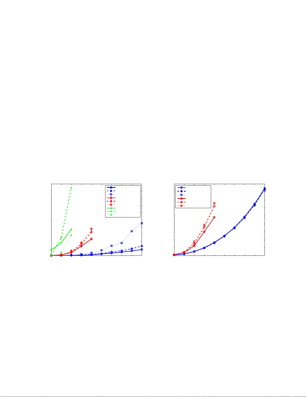
Supp ort V ector Mac hine Classi fi cation with Indefinite Ke rnels Ronn y Luss ∗ Alexandre d’Aspremon t † Ma y 22, 2018 Abstract W e prop ose a metho d for supp ort vector machine classificatio n using indefinite k ernels. In- stead of dir ectly minimizing or stabilizing a no ncon v ex loss function, our algo rithm simultane- ously computes supp ort v ectors and a proxy kernel matr ix used in fo rming the loss. This can be int erpreted as a p enalized kernel learning pro blem where indefinite k ernel matr ices ar e treated as noisy obser v ations of a true Mercer k ernel. Our form ulation keeps the problem con v ex and relatively lar ge problems can b e solved efficiently using the pr o jected gradient or analytic cen ter cutting plane metho ds . W e co mpare the perfo r mance of o ur technique with other methods on several s tandard data s ets. 1 In tro d uction Supp ort v ector mac hines (SVM) ha ve become a cen tral to ol for solving binary classification prob- lems. A critical step in sup p ort v ector mac h in e classificatio n is c ho osing a suitable kernel matrix, whic h mea sures simila rit y b et ween data p oin ts and m ust b e p ositiv e semidefinite b ecause it is formed as the Gram matrix of data p oin ts in a repro ducing k ernel Hilb ert space. This p ositiv e semidefinite condition on kernel matrices is also kn own as Mercer’s cond itio n in the mac hine learn- ing literature. The classification prob lem then b ecomes a linearly constrained quadratic program. Here, we pr esen t an algorithm for SVM classification using indefinite ke rnels 1 , i.e. kernel matrices formed using similarit y m easures wh ic h are n ot p o sitiv e semidefinite. Our in terest in indefinite k ernels is motiv ated b y seve ral observ ations. First, certain similar- it y measures tak e adv ant age of application-sp ecific structur e in the d ata and often d ispla y excel- len t empirical classification p erformance. Unlik e p opular k ernels used in supp ort vect or mac hine classification, these similarit y matrices are often indefi n ite, so do not necessarily corr esp on d to a repro ducing kernel Hilb ert space. (S ee Ong et al. (20 04) for a discussion.) In p articular, an application of classification with ind efinite k ernels to image classification us- ing Earth Mo ver’s Distance w as discussed in Zamolotskikh and Cun ningham (200 4). Similarit y measures for protein sequences such as the Smith-W aterman and BLAST scores are indefin ite y et ha v e provided hin ts for constructing useful p ositiv e semidefin ite kernels suc h as th ose decrib ed in Saigo et al. (2004) or hav e been transf orm ed into p ositiv e semidefin ite k ernels w ith go od empirical p erformance (see L anc kriet et al. (2003), for example). T angen t distance similarity measures, as ∗ ORFE Dep artmen t, Princeton Universit y , Princeton, N J 08544 . rluss@a lumni.pri nceton.edu † ORFE Dep artmen t, Princeton Universit y , Princeton, N J 08544 . aspremo n@princet on.edu 1 A preliminary versio n of t his pap er app eared in the pro ceedings of t he Neural In forma tion Processing Systems (NIPS) 2007 conference and is av ailable at http://book s.nips.cc/ nips20.html 1 describ ed in Simard et al. (1 998) or Haasdonk and Keysers (2002), are inv arian t to v arious simp le image transformations and ha v e also shown excellen t p erform an ce in optical c haracter recognition. Finally , it is sometimes imp ossible to prov e that s ome k ernels satisfy Mercer’s condition or the n umerical complexit y of ev aluating th e exact p ositive k ernel is too high and a pro xy (and not necessarily p ositive semidefin ite) kernel has to b e u sed instead (see Cutu ri (2007 ), for example). In b oth cases, our method allo ws us to b ypass these limitations. Our ob jec tiv e here is to derive efficien t algorithms to d irectly use these indefi n ite similarit y measur es for cla ssification. Our work closely follo ws, in spirit, recen t results on k ernel lea rning (see Lanckriet et al. (2004 ) or Ong et al. (2005)), wh ere th e k ernel matrix is learned as a linear combination of giv en k ernels, and the result is explicitly constrained to b e p ositiv e s emid efinite. W hile this problem is numerically c h allenging, Bac h e t al. (2004) a dapted the SMO algorithm to solve the case where the kernel is w ritten as a p ositive ly w eigh ted com bination o f other k er n els. I n our setting h ere, we never numeric al ly optimize the k ernel matrix b ecause this part of the problem can b e solv ed explicitly , whic h means that the complexit y of our method is sub stan tially lo wer than that of classical k ernel learning algorithms and closer in practice to the algorithm used in S onnen b erg et al. (2006) , who form ulate the m ultiple k ernel learning problem of Bac h et al. (2004 ) as a s emi-infinite linear p rogram and solv e it with a column generation tec hnique similar to the analytic cente r cutting p lane m ethod w e u se here. 1.1 Curren t r esults Sev eral methods ha ve b een prop osed for dealing w ith indefin ite kernels in SVMs. A first direction em b eds data in a p seudo-Euclidean (pE) space: Haasdonk (2005), for exa mple, formulat es th e classification problem w ith an indefinite kernel as that of minimizing the d istance b et w een conv ex h ulls form ed fr om the t wo categories of data em b edded in the pE sp ace. T he n onseparable case is handled in th e same mann er us in g r ed uced con v ex hulls. (See Bennet and Bredensteiner (2000) for a discussion on geo metric in terp retati ons in SVM.) Another direction applies direct sp ectral transf ormations to indefinite kernels: flipping the n eg- ativ e eigen v alues or shifting the eigen v alues and reconstru cting the kernel with the original eigen- v ecto rs in order to p rod uce a p o sitiv e semidefinite ke rnel (see W u et al. (2005) and Zamolotskikh and Cunn ingham (2004), for example). Y et another option is to reformulate either the maxim u m margin problem or its du al in order to use the indefinite k ern el in a co n v ex optimization problem. One r eform u lation suggested in Lin and Lin (200 3) replaces the indefi n ite k ernel by the identit y matrix and mainta ins separation u s ing linear constraints. This metho d achiev es go od p erformance, but th e con v exificatio n pr ocedu r e is h ard to interpret. Directly solving the nonconv ex pr oblem sometimes giv es go o d results as we ll (see W o ´ znica et al. (2006) and Haasdonk (2005)) b u t offers no guaran tees on p erformance. 1.2 Con tributions In this w ork, instead of directly transforming the indefinite k ern el, w e simulta neously learn the supp ort v ector w eigh ts and a pro xy Mercer k ernel matrix b y p enalizing the distance b e t ween this pro xy k ernel and the original, indefinite one. Our main result is that the k ernel learning part of that problem can b e solved explicitly , mea ning that the classificatio n problem with indefinite k ernels can simply b e formulated as a p er tu rbation of the p o sitiv e semidefinite case. 2 Our formulation can b e in terpreted as a p enalized k ernel learnin g problem w ith uncertain t y on the input kernel matrix. In that sense, indefinite similarit y matrices are seen as noisy observ a- tions of a tru e p ositive semidefinite ke rnel and we learn a k ernel th at increases the generalizatio n p erformance. F rom a complexit y standp oin t, while the original SVM classificat ion problem with indefinite kernel is nonconv ex, the p enalizatio n w e detail h ere results in a con vex p roblem, an d hence can b e solve d efficien tly with guaran teed complexit y b ounds. The paper is organized as f ollo ws. In Section 2 w e formulate our main classification result and detail its inte rpretation as a p enalized kernel learning problem. In Section 3 we describ e three algorithms for s olving this p roblem. Section 4 discusses seve ral extensions of our main results. Finally , in S ectio n 5, we test the numerical p erformance of these method s on v arious data sets. Notation W e write S n ( S n + ) to denote the set of symmetric (p ositive -semidefinite) matrice s of s ize n . The v ecto r e is th e n -v ecto r of ones. Give n a matrix X , λ i ( X ) d enotes the i th eigen v alue of X . X + is th e p ositiv e p art of the m atrix X , i.e. X + = P i max(0 , λ i ) v i v T i where λ i and v i are the i th eigen v alue and eigen vec tor of the matrix X . Given a v ecto r x , k x k 1 = P | x i | . 2 SVM with indefinite k ernels In th is section, w e mo dify the SVM k ernel le arning problem and formulat e a p enalized k ernel learning p roblem on indefin ite k er n els. W e also detail h o w our framewo rk applies to kernels that satisfy Merce r’s condition. 2.1 Kernel learning Let K ∈ S n b e a given kernel matrix and let y ∈ R n b e the vec tor of lab els, with Y = diag ( y ), the matrix with diagonal y . W e form ulate the k ern el learning p roblem as in Lanckriet et al. (200 4), where the authors minimize an upp er b oun d on th e misclassification probabilit y when using S VM with a giv en kernel K . This upp er b oun d is th e generalized p erformance measure ω C ( K ) = max { 0 ≤ α ≤ C,α T y = 0 } α T e − T r ( K ( Y α )( Y α ) T ) / 2 (1) where α ∈ R n and C is the SVM misclassification p enalt y . This is also the classic 1-norm soft margin S VM prob lem. They sho w that ω C ( K ) is conv ex in K and solv e problems of the form min K ∈K ω C ( K ) (2) in order to learn an optimal k ernel K ∗ that ac hiev es goo d generalizat ion p erforman ce. When K is restricted to con v ex subsets of S n + with constan t trace, they sho w that problem (2) can b e reform ulated as a con ve x program. F urther restrictions to K r educe (2) to more tractable optimization p r oblems suc h as semidefinite and quadratically constrained qu adratic programs. Our goal is to solv e a problem similar to (2) b y restricting the distance b et w een a pro xy k ernel used in classification and the original indefin ite similarit y measur e. 3 2.2 Learning from indefinite k ernels The p erformance m easur e in (1) is the d ual of the SVM classifica tion problem with h inge loss and quadratic p en alty . When K is p ositiv e semidefinite, this pr ob lem is a con vex qu adratic program. Supp ose n o w that we are giv en an indefinite k ern el matrix K 0 ∈ S n . W e formulate a new instance of problem (2) b y restricting K to b e a p ositiv e semidefinite k ern el matrix in some giv en n eig h b orho o d of the original (indefinite) ke rnel matrix K 0 and solv e min { K  0 , k K − K 0 k 2 F ≤ β } max { α T y = 0 , 0 ≤ α ≤ C } α T e − 1 2 T r ( K ( Y α )( Y α ) T ) in the v ariables K ∈ S n and α ∈ R n , where the parameter β > 0 con trols the distance b et wee n the o riginal matrix K 0 and th e pro xy k ernel K . This is the kernel learning problem (2) with K = { K  0 , k K − K 0 k 2 F ≤ β } . T he ab o ve p roblem is infeasible f or small v alues of β , so we replace here the h ard constraint on K by a p enalt y ρ on the distance b et w een the pr o xy kernel and the original indefinite similarit y matrix and solv e instead min { K  0 } max { α T y = 0 , 0 ≤ α ≤ C } α T e − 1 2 T r ( K ( Y α )( Y α ) T ) + ρ k K − K 0 k 2 F (3) Because (3) is con v ex-conca v e and the inn er maximization has a compact feasible set, w e can switc h the max and min to form the dual max { α T y = 0 , 0 ≤ α ≤ C } min { K  0 } α T e − 1 2 T r ( K ( Y α )( Y α ) T ) + ρ k K − K 0 k 2 F (4) in th e v ariables K ∈ S n and α ∈ R n . W e first note that problem (4) is a conv ex optimization problem. Th e inner minimization problem is a con v ex conic program on K . Also, as th e p oin t wise minim um of a family of conca ve quadratic functions of α , the solution to the inn er pr oblem is a conca ve fun ctio n of α , hence the outer optimization problem is also con v ex (see Bo yd and V and en b erghe (2004) for fur ther details). Th us, (4) is a conca ve maximization problem sub ject to lin ear constraints and is therefore a con v ex problem in α . Our key result here is that the inner k ernel learning op timization prob lem in (4) can b e solve d in closed form. Theorem 1 Given a similarity matrix K 0 ∈ S n , a ve ctor α ∈ R n of supp ort ve ctor c o efficients and the lab el matr ix Y = diag ( y ) , the optimal k e rnel in pr oblem (4) c an b e c ompute d explicitly as: K ∗ = ( K 0 + ( Y α )( Y α ) T / (4 ρ )) + (5) wher e ρ ≥ 0 c ontr ols the p enalty. Pro of. F or a fixed α , the inner minimization problem can b e wr itten out as min { K  0 } α T e + ρ ( T r ( K T K ) − 2 T r ( K T ( K 0 + 1 4 ρ ( Y α )( Y α ) T )) + T r ( K T 0 K 0 )) where we ha v e replaced k K − K 0 k 2 F = T r (( K − K 0 ) T ( K − K 0 )) and collect ed sim ilar terms. Adding and subtracting the constan t ρ T r (( K 0 + 1 4 ρ ( Y α )( Y α ) T ) T ( K 0 + 1 4 ρ ( Y α )( Y α ) T )) sho ws that the inner minimization problem is equiv alen t to the pr ob lem minimize k K − ( K 0 + 1 4 ρ ( Y α )( Y α ) T ) k 2 F sub ject to K  0 4 in the v ariable K ∈ S n , where w e ha ve dropp ed the remaining constan ts from the ob jectiv e. This is the pro jection of the matrix K 0 + ( Y α )( Y α ) T / (4 ρ ) on the cone of p ositiv e semidefin ite m atrice s, whic h yields the d esired result. Plugging th e explicit solution for the pr o xy k ern el derived in (5) int o the classificatio n pr ob- lem (4), w e get max { α T y = 0 , 0 ≤ α ≤ C } α T e − 1 2 T r ( K ∗ ( Y α )( Y α ) T ) + ρ k K ∗ − K 0 k 2 F (6) in the v ariable α ∈ R n , where ( Y α )( Y α ) T is the rank one matrix w ith co efficien ts y i α i α j y j . Problem (6) can b e cast as an eigen v alue optimization pr oblem in the v ariable α . Letting th e eigen v alue decomp osition of K 0 + ( Y α )( Y α ) T / (4 ρ ) b e V D V T , we get K ∗ = V D + V T , and with v i the i th column of V , w e can wr ite T r ( K ∗ ( Y α )( Y α ) T ) = ( Y α ) T V D + V T ( Y α ) = X i max  0 , λ i  K 0 + 1 4 ρ ( Y α )( Y α ) T  ( α T Y v i ) 2 . Using the same tec hnique, w e can also rewr ite th e term k K ∗ − K 0 k 2 F using this eigen v alue decom- p osition. Our original optimizati on problem (4) fin ally b ecomes maximize α T e − 1 2 P i max(0 , λ i ( K 0 + ( Y α )( Y α ) T / 4 ρ ))( α T Y v i ) 2 + ρ P i (max(0 , λ i ( K 0 + ( Y α )( Y α ) T / 4 ρ ))) 2 − 2 ρ P i T r (( v i v T i ) K 0 )max(0 , λ i ( K 0 + ( Y α )( Y α ) T / 4 ρ )) + ρ T r ( K 0 K 0 ) sub ject to α T y = 0 , 0 ≤ α ≤ C (7) in the v ariable α ∈ R n . By construction, the ob jectiv e function is conca ve, hence (7) is a conv ex optimization problem in α . A reform ulation of problem (4) app ears in C hen and Y e (200 8) wh ere the authors mov e the inner minimization problem to the co nstrain ts a nd ge t the follo wing semi-infinite quad r atic ally constrained linear program (SIQCLP): maximize t sub ject to α T y = 0 , 0 ≤ α ≤ C t ≤ α T e − 1 2 T r ( K ( Y α )( Y α ) T ) + ρ k K − K 0 k 2 F ∀ K  0 . (8) In Section 3, we describ e algorithms to solv e our eigen v alue optimizati on p roblem in (7 ), as w ell as an algo rithm fr om Ch en and Y e (2008) that solv es the differen t f ormulation in (8 ), for completeness. 2.3 In terpretation Our explicit solution of the optimal k ern el giv en in (5) is th e pro j ecti on of a p enalize d r ank-one up date to the indefinite k ernel on the cone of p ositiv e s emidefinite matrices. As ρ tends to infinity , the rank -one up date has less effect and in the limit, the optimal k ernel is give n b y zeroing out the 5 negativ e eigen v alues of the indefinite k ern el. This means that if th e in definite kernel con tains a v ery small amount of n oise, the b est p ositiv e semidefinite k ernel to use with SVM in our f ramew ork is the p ositiv e part of the indefinite k ern el. This limit as ρ tends to infinit y also motiv ates a heuristic f or trans forming the ke rnel on the testing s et. Since negativ e eig en v alues in the training k ernel are thr esh olded to zero in the limit, the same tran s formation shou ld o ccur for the test ke rnel. Hence, to measure generalization p erfor- mance, w e up d ate the en tries of the full kernel corresp onding to training instances by the rank-one up date resulting from the optimal solution to (7) and threshold th e negativ e eigen v alues of the fu ll k ernel m atrix to zero to pro duce a Merce r k ern el on the test set. 2.4 Dual problem As discus sed ab o v e, p roblems (3) and (4) are du al. Th e inner maximization in p roblem (3) is a quadratic program in α , whose dual is the qu adratic minimization problem minimize 1 2 ( e − δ + µ + y ν ) T ( Y K Y ) − 1 ( e − δ + µ + y ν ) + C µ T e sub ject to δ , µ ≥ 0 . (9) Substituting (9 ) for the in ner maximization in p roblem (3) allo ws us to wr ite a join t minimization problem minimize T r ( K − 1 ( Y − 1 ( e − δ + µ + y ν ))( Y − 1 ( e − δ + µ + y ν )) T ) / 2 + C µ T e + ρ k K − K 0 k 2 F sub ject to K  0 , δ, µ ≥ 0 (10) in the v ariables K ∈ S n , δ, µ ∈ R n and ν ∈ R . T his is a qu adratic program in the v ariables δ , µ (whic h corresp ond to the constrain ts 0 ≤ α ≤ C ) and ν (whic h is the dual v ariable for the constraint α T y = 0) . As w e hav e seen earlier, any feasible solution α ∈ R n pro duces a corr esp on d ing pro xy k ernel in (5). Plugging this kernel into problem (10) allo ws us to compute an upp er bou n d on the optim um v alue of problem (4) by solving a s imple q u adratic p r ogram in the v ariables δ, µ, ν . Th is result can then b e used to b ound the dualit y gap in (7) and trac k con vergence. 3 Algorithms W e now detail t w o algorithms that can b e used to solv e problem (7), which maximizes a n ondiffer- en tiable conca ve fun ction s ub ject to conv ex constrain ts. An optimal p oin t alw a ys exists since th e feasible set is b ounded and non emp t y . F or numerical stabilit y , in b oth algorithms, w e quadratically smo oth our ob jectiv e to compu te a gradient . W e fi rst describ e a simple pro jected gradien t m ethod whic h has numerically c h eap iterations but less pr ed icta ble p erf orm ance in pr acti ce. W e then sho w ho w to ap p ly the analytic cente r cutting p lane metho d, whose iterations are numerically m ore com- plex bu t w h ic h con verges linearly . F or completeness, w e also describ e an exchange metho d from Chen and Y e (2008) used to solv e p roblem (8), where the n umerical b ottlenec k is a quadr atic ally constrained linear program solv ed at eac h iteratio n. Smo othing Our ob jectiv e cont ains terms of the form max { 0 , f ( x ) } for some function f ( x ), whic h are not d ifferentiable (d escrib ed in the section b elow). These f u nctions are ea sily smo othed out by 6 a Moreau-Y osid a regularization technique (see Hiriart-Urrut y and Lemar ´ ec hal (1993), for example). W e replace th e max b y a contin uously differenti able ǫ 2 -appro ximation as follo ws: ϕ ǫ ( f ( x )) = max 0 ≤ u ≤ 1 ( uf ( x ) − ǫ 2 u 2 ) . The gradien t is th en giv en by ∇ ϕ ǫ ( f ( x )) = u ∗ ( x ) ∇ f ( x ) where u ∗ ( x ) = argmax ϕ ǫ ( f ( x )). Gradien t Calculating the gradien t of the ob jectiv e function in (7) requires computing the eigen- v alue decomp ositio n of a m atrix of the form X ( α ) = K + ραα T . Giv en a matrix X ( α ), the d eriv ativ e of the i th eigen v alue with resp ect to α is then gi v en b y ∂ λ i ( X ( α )) ∂ α = v T i ∂ X ( α ) ∂ α v i (11) where v i is the i th eigen vect or of X ( α ). W e can then combine this expression with the smo oth appro ximation ab ov e to obtain the gradient. 3.1 Computing pro xy kernels Because the proxy kernel in (5) only requir es a rank one u p date of a (fixed) eigen v alue d ecomp osition K ∗ = ( K 0 + ( Y α )( Y α ) T / (4 ρ )) + , w e no w br iefly recall ho w v i and λ i ( X ( α )) can b e computed efficien tly in this case (see Demmel (1997 ) for further details). W e refer the reader to Kulis et al. (2006) for another kernel learning example using this metho d. Giv en the eigen v alue d ecomposition X = V D V T , by changing basis this prob lem can b e reduced to th e d eco mp osition of th e diagonal plus r ank-one matrix, D + ρuu T , where u = V T α . First, the up d ate d eigen v alues are d etermined by solving the secular equations det( D + ρuu T − λI ) = 0 , whic h can b e done in O ( n 2 ). While there is an explicit solution for the eigen v ecto rs corresp ond ing to these eigen v alues, they are not stable b ecause th e eigen v alues are app ro ximated. This in s tabilit y is circum v ented by computing a v ector ˆ u such that appr o ximate eigen v alues λ are the exact eigen v alues of the matrix D + ρ ˆ u ˆ u T , then computing its stable eigen ve ctors explicitly , where b oth s teps can b e done in O ( n 2 ) time. The ke y is that D + ρ ˆ u ˆ u T is close enough to our original matrix so that the eigen v alues and eigen vect ors are stable app r o ximations of the true v alues. Final ly , t he eigen vect ors o f our original matrix are computed as V W , w ith W as the stable eigen ve ctors of D + ρ ˆ u ˆ u T . Up dating the eigenv alue decomp osition is reduced to an O ( n 2 ) pro cedure plus one matrix m ultiplication, whic h is then the complexit y of one gradien t compu tat ion. W e n ote that eige n v alues of symm etric matrices are not d ifferentiable when some of them ha v e m ultiplicities greater th an one (see Overto n (1992) for a discussion), but a subgrad ient can b e u sed instead of the gradien t in all the algorithms detailed here. Lewis (19 99) s ho ws ho w to compu te an appro ximate su b differen tial of the k-th largest eigen v alue of a symmetric matrix. This can th en b e used to form a regular subgradient of the ob jectiv e f unction in (7) whic h is conca v e by construction. 7 Algorithm 1 Pro jected gradien t metho d 1: Comp ute α i +1 = α i + t ∇ f ( α i ). 2: S et α i +1 = p A ( α i +1 ). 3: If gap ≤ ǫ stop, otherwise go bac k to s tep 1. 3.2 Pro jected gradien t metho d The pro jected gradient method tak es a steep est descen t step, then pro jects the new p oin t bac k on to the feasible region (see Bertsek as (1999), for example). W e c ho ose an initial p oin t α 0 ∈ R n and the algorithm pro ceeds as in Algorithm 1 . Here, w e ha v e assumed that the ob jectiv e f u nction is differenti able (after smoothing). The metho d is only efficien t if the p r o jection step is numericall y c heap. Th e complexit y of eac h iteration then b reaks do wn as follo ws: Step 1. Th is requires an eigen v alue decomp osition that is computed in O ( n 2 ) plus one matrix m ultiplicatio n as describ ed ab o v e. Exp er im ents b elo w use a stepsize of 5 /k for In definiteSVM and 10 /k for P erturbSVM (describ ed in Section 4.3) wh ere k is the iteration num b er. A go od stepsize is crucial to p erformance, and m ust b e chosen separately for eac h data set as there is no rule of th um b. W e note that a line searc h would b e costly here b ecause it would r equire multiple eige n v alue decomp ositions to recalculate the ob j ect iv e m ultiple times. Step 2. This is a p r o jection on to the region A = { α T y = 0 , 0 ≤ α ≤ C } and can b e solv ed explicitly b y sorting the v ector of entries, w ith cost O ( n lo g n ). Stopping Criterion. W e can compute a dualit y gap using the results of § 2.4 wh ere K i = ( K 0 + ( Y α i )( Y α i ) T / (4 ρ )) + is the candidate k ernel at iteration i and w e solv e problem (1), w hic h simply means solving a SVM problem with the p ositiv e semidefinite k ern el K i , and pro duces an u pp er b ound on (7), hence a b ound on the sub optimalit y of the current solution. Complexity. The n um b er of iterations required by this metho d to r eac h a target precision of ǫ gro w s as O (1 /ǫ 2 ). See Nest ero v (2003) for a complete discussion. 3.3 Analytic cen ter cutting plane metho d The analytic cen ter cutting plane m ethod (ACCPM) reduces th e feasible r egi on at eac h iteration using a n ew cut computed by ev aluating a subgrad ient of the ob jectiv e fun ction at the analytic cen ter of the curr en t feasible set, until the v olume of the reduced region conv erges to th e target precision. This method do es not require differentia bilit y . W e set L 0 = { x ∈ R n | x T y = 0 , 0 ≤ x ≤ C } , which we can write as { x ∈ R n | A 0 x ≤ b 0 } , to b e our first lo calizat ion set for the optimal solution. The metho d is described in Algorithm 2 (see Bertsek as (1999 ) for a more complete treatmen t of cutting plane metho ds). The co mplexit y of eac h iteration breaks d o wn as foll o w s: Step 1. This step computes th e analytic cen ter of a p olyhedr on and can b e solv ed in O ( n 3 ) op erations u sing int erior p oin t methods , for examp le. Step 2. This s im p ly u p dates the p olyhedral description. It includ es the gradien t computation whic h again is O ( n 2 ) plus one matrix multiplica tion. 8 Algorithm 2 Analytic cent er cutting plane metho d 1: Comp ute α i as the analytic ce n ter of L i b y solving x i +1 = argmin x ∈ R n − m X i =1 log( b i − a T i x ) where a T i represent s the i th ro w of co efficien ts from the left-hand side of { x ∈ R n | A i x ≤ b 0 } . 2: Comp ute ∇ f ( x ) at the cen ter x i +1 and up date the (p olyhedr al) lo caliza tion set L i +1 = L i ∩ {∇ f ( x i +1 )( x − x i +1 ) ≥ 0 } where f is ob jectiv e in pr oblem (7). 3: If m ≥ 3 n , reduce the num b er of constrain ts to 3 n . 4: If gap ≤ ǫ stop, otherwise go bac k to s tep 1. Step 3. This step requires ordering the constrain ts according to their relev ance in the localization set. One r elev ance measure for the j th constrain t at iteration i is a T j ∇ 2 f ( x i ) − 1 a j ( a T j x i − b j ) 2 (12) where f is the ob jectiv e function of the analytic cen ter problem. C omputing the hessian is easy: it requires matrix m u ltiplicat ion of the form A T D A where A is m × n (matrix m ultiplicatio n is k ept inexp ensiv e in this step by p runing redundant constraints) and D is diagonal. R estricting the n u m b er of constrain ts to 3 n is a rule of th u mb; r aising this limit increases the p er iteration complexit y wh ile d ecreasing it increases the required n u m b er of iterations. Stopping Criterion. An upp er b ound is computed b y maximizing a fi rst ord er T a ylor appr o ximation of f ( α ) at α i o ver all p oin ts in an ell ipsoid that co v ers A i , whic h can be co mputed explicitly . Complexity. A CCPM is pro v ably con v ergen t in O ( n (log 1 /ǫ ) 2 ) iterations when u sing cut elimina- tion, whic h ke eps th e complexit y of the lo calizati on set b ounded . O ther sc hemes are a v ailable w ith sligh tly different complexitie s: a b ound of O ( n 2 /ǫ 2 ) is ac hiev ed in Goffin and Vial (2002) usin g (c h eaper) approxi mate cen ters, for example. 3.4 Exc hange met ho d for SIQCLP The algorithm considered in Ch en and Y e (2008) in order to solve p roblem (8) falls un der a class of algorithms calle d exc hange metho ds (as defined in Hettic h and Kortanek (1993 )). Th ese methods iterativ ely solv e p roblems constrained b y a finite subset of the infin itely man y constraints, w here the s olution at eac h ite rate giv es an improv ed lo wer b ound to the maximization pr oblem. The subpr oblem solve d at eac h iteratio n here is maximize t sub ject to α T y = 0 , 0 ≤ α ≤ C t ≤ α T e − 1 2 T r ( K i ( Y α )( Y α ) T ) + ρ k K i − K 0 k 2 F i = 1 , . . . , p (13) 9 where p is the num b er of constrain ts used to appro ximate th e infi nitely many constrain ts of pr oblem (8). L et ( t 1 , α 1 ) b e an initial solution found by solving prob lem (13) with p = 1 and K 1 = ( K 0 ) + , where K 0 is the input in definite ke rnel. Th e algorithm pro ceeds as in Algorithm 3 b elo w. Algorithm 3 Exc hange metho d 1: Comp ute K i +1 b y solving the inner minimization problem of (4) as a fu nction of α i . 2: S top if α T i e − 1 2 T r ( K i +1 ( Y α i )( Y α i ) T ) + ρ k K i +1 − K 0 k 2 F ≥ t i . 3: S olv e p roblem (13) with an additional constraint us in g K i +1 to get ( t i +1 , α i +1 ) and go b ack to step 1. The co mplexit y of eac h iteration breaks d o wn as foll o w s: Step 1. T his step can b e solv ed analytically using Theorem 1. An efficient calculation of K i +1 can b e made as in the other algorithms ab o ve using an O ( n 2 ) p rocedu re plus one matrix m ultiplication. Step 2 (Stopping Criterion). The p r evious p oin t ( t i , α i ) is optimal if it is feasible with r esp ect to the new constrain t, in wh ic h case it is feasible for the infinitely many constraints of the original problem (8) and hence also optimal. Step3. Th is step requires s olving a QCLP with a n umber of qu adratic constraints equiv alen t to th e n um b er of ite rations. As shown in Chen and Y e (2008), the QCLP can b e written as a regularized v ersion of the multiple kernel learning (MKL) problem fr om Lanc kriet et al. (2004 ), where the n um b er of constrain ts here is equiv alen t to the num b er of kernels in MKL. Efficien t method s to solv e MKL with man y kernels is an activ e area of researc h, m ost recent ly in Rak otoma monjy et al. (2008 ). There, the authors use a gradien t m etho d to solv e a reform ulation of problem (13 ) as a smo oth maximization problem. Eac h ob jectiv e v alue and gradient computation requires compu ting a su p p ort v ecto r mac hine, hence eac h iteratio n r equ ires sev eral SVM compu tati ons whic h can b e sp eeded up using warm-starting. F u r thermore, Chen an d Y e (2008) prune inactiv e constrain ts at eac h iteration in order to decrease the num b er of constrain ts in the QCLP . Complexity. No r ate of con vergence is kn own for this algorithm, but the dualit y gap giv en in Chen and Y e (2008) is sho wn to monotonically decrease. 3.5 Matlab Implemen tation The first t w o al gorithms discu s sed here we re implemented in Matlab for the cases of indefin ite (IndefiniteSVM) and p ositiv e semid efinite (PerturbSVM) k ernels and ca n b e d ownloaded f r om the authors’ we bpages in a pac k age called In definiteSVM. Th e ρ p enalt y parameter is one-dimen s ional in the implemen tation. This pac k age mak es use of the LIBSVM code of Chang and Lin (2001 ) to pro duce sub optimalit y b ound s and trac k conv ergence. A Matlab implementa tion of th e exc hange metho d (due to the authors of Chen and Y e (200 8)) that uses MOSEK (MOSEK ApS 2008) to solv e pr oblem (13) is compared ag ainst the pro jected gradien t metho d in Section 5. 4 Extensions In this section, we extend our results to other k ernel metho ds, namely su pp ort v ector regressions and one-c lass supp ort ve ctor mac hines. In addition, w e app ly our metho d to using Mercer ke rnels 10 and sho w ho w to use more general p enalties in our form u lati on. 4.1 SVR with indefi nite kerne ls The practicalit y of indefinite k ernels in S VM classificatio n similarly motiv ates u sing indefinite k ernels in supp ort vec tor regression (SVR). W e here exte nd the formulati ons in Section 2 to S VR with lin ear ǫ -insensitive loss ω C ( K ) = max {− C ≤ α ≤ C, α T e =0 } α T y − ǫ | α | − T r ( K αα T ) / 2 (14) where α ∈ R n and C is the SVR p enalt y parameter. The in definite SVR formulation follo ws directly as in Section 2.2 and the optimal kernel is learned by solving max { α T e =0 , − C ≤ α ≤ C } min { K  0 } α T y − ǫ | α | − 1 2 T r ( K αα T ) + ρ k K − K 0 k 2 F (15) in the v ariables K ∈ S n and α ∈ R n , where the parameter ρ > 0 cont rols the magnitude of th e p enalt y on the distance b et w een K and K 0 . The f ollo wing corollary to T heorem 1 pro vides the solution to the inner minimization problem in (15) Corollary 2 Given a similarity matrix K 0 ∈ S n and a ve ctor α ∈ R n of supp ort ve ctor c o efficients, the optimal kernel in pr oblem (15) c an b e c ompute d explicitly as K ∗ = ( K 0 + αα T / (4 ρ )) + (16) wher e ρ ≥ 0 c ontr ols the p enalty. The proof follo ws dir ect ly as in Theorem 1; the sligh t difference is that the v ector of labels y do es not app ear in the optimal k ernel. Plugging in (16) into (15), the resulting form ulation can b e rewritten as the con vex eigenv al ue optimization problem maximize α T y − ǫ | α | − 1 2 P i max(0 , λ i ( K 0 + αα T / (4 ρ )))( α T v i ) 2 + ρ P i (max(0 , λ i ( K 0 + αα T / 4 ρ ))) 2 − 2 ρ P i T r (( v i v T i ) K 0 )max(0 , λ i ( K 0 + αα T / (4 ρ ))) + ρ T r ( K 0 K 0 ) sub ject to α T e = 0 , − C ≤ α ≤ C (17) in the v ariable α ∈ R n . Again, a pr o xy k ern el giv en by (16) can b e pr od uced from any feasible solution α ∈ R n . Plugging the p ro xy ke rnel in to pr oblem (15) allo ws us to compute an upp er b ound on the optimum v alue of p roblem (15) b y solving a sup p ort v ector regression pr oblem. 4.2 One-class SVM with indefi nite ke rnels The same r eform u lation can also b e applied to one-class su pp ort v ector mac hines wh ic h ha v e the form ulation (see Sc h¨ o lk opf and Smola (20 02)) ω ν ( K ) = max { 0 ≤ α ≤ 1 ν l ,α T e =1 } − T r ( K αα T ) / 2 (18) 11 where α ∈ R n , ν is the one-class SVM parameter, and l is the n u m b er of training p oin ts. The indefinite one-c lass SVM form ulation f ollo ws agai n as done for binary SVM and SVR; the optimal k ernel is learned b y solving max { α T e =1 , 0 ≤ α ≤ 1 ν l } min { K  0 } − 1 2 T r ( K αα T ) + ρ k K − K 0 k 2 F (19) in the v ariables K ∈ S n and α ∈ R n . The inn er minimization p roblem is identi cal to that of indefinite SVR and the optimal kernel h as the same form as give n in Corollary 2. Plu gging (16) in to (19 ) giv es another con v ex eigen v alue optimizatio n problem maximize − 1 2 P i max(0 , λ i ( K 0 + αα T / 4 ρ ))( α T v i ) 2 + ρ P i (max(0 , λ i ( K 0 + αα T / (4 ρ )))) 2 − 2 ρ P i T r (( v i v T i ) K 0 )max(0 , λ i ( K 0 + αα T / (4 ρ ))) + ρ T r ( K 0 K 0 ) sub ject to α T e = 1 , 0 ≤ α ≤ 1 ν l (20) in the v ariable α ∈ R n , whic h is identic al to (17) without the first t w o terms in th e ob jectiv e and slig h tly differen t constraints. The alg orithm follo ws almost directly the same as ab ov e for the indefinite SVR formulat ion. 4.3 Learning from Mercer k ernels While our cen tral motiv ation is t o use indefinite k er n els for SVM classificatio n, one wo uld also lik e to anal yze what happ ens wh en a Mercer k ern el is used as input in (4). I n this case, w e learn another k ernel that decreases the upp er b ound on generaliza tion p erformance and pro duces p erturb ed sup p ort v ecto rs. W e can again in terpret the input as a noisy kernel, and as such, one that will ac h iev e sub optimal p erformance. If the input k ernel is the b est k ernel to use (i.e. is not noisy), we will observe that our fr amew ork ac hiev es optimal p erformance as ρ tends to infinit y (through cross v alidation), otherwise w e simply learn a b etter ke rnel using a finite ρ . When the similarit y measure K 0 is p ositiv e semidefinite, th e pro xy kernel K ∗ in Theorem 1 simplifies to a rank-one up date of K 0 K ∗ = K 0 + ( Y α ∗ )( Y α ∗ ) T / (4 ρ ) (21) whereas, for ind efi nite K 0 , the solution was to pro ject this matrix on the cone of p ositive semidefi n ite matrices. Plugging (21) into problem (4) giv es: max { α T y = 0 , 0 ≤ α ≤ C } α T e − 1 2 T r ( K 0 ( Y α )( Y α ) T ) − 1 16 ρ X i,j ( α i α j ) 2 , (22) whic h is the classic SVM problem give n in (1) with a fourth order p enalt y on the sup p ort v ectors. F or testing in this framew ork , we do not need to transf orm the kernel, only the supp ort v ectors are p erturb ed. In this case, computing the gradien t n o longer requires eigenv alue decomp ositions at eac h iteration. Exp eriment al r esults are sho wn in Section 5. 12 4.4 Comp onen twise penalties Indefinite SVM can b e generaliz ed fur ther w ith comp onent wise p enalties on the distance b et w een the pro xy k ernel and the ind efinite k ernel K 0 . W e generalize problem (4) to max { α T y = 0 , 0 ≤ α ≤ C } min { K  0 } α T e − 1 2 T r ( K ( Y α )( Y α ) T ) + X i,j H ij ( K ij − K 0 ij ) 2 (23) where H is now a matrix of v arying p enalties on the comp onen twise distances. F or a sp ecific class of p enaltie s, the optimal k ern el K ∗ can b e deriv ed explicitly as follo w s. Theorem 3 Given a similarity matrix K 0 ∈ S n , a ve ctor α ∈ R n of supp ort ve ctor c o efficients and the lab el matrix Y = dia g ( y ) , when H is r ank-one with H ij = h i h j , the optimal kernel in pr oblem (23) has the explicit form K ∗ = W − 1 / 2 (( W 1 / 2 ( K 0 + 1 4 ( W − 1 Y α ∗ )( W − 1 Y α ∗ ) T ) W 1 / 2 ) + ) W − 1 / 2 (24) wher e W i s the diagonal matrix with W ii = h i . Pro of. T h e inner minimization pr oblem to p roblem (23) can b e written out as min { K  0 } X i,j H ij ( K 2 ij − 2 K ij K 0 ij + K 2 0 ij ) − 1 2 X i,j y i y j α i α j K i,j . Adding and su btracting P i,j H ij ( K 0 ij + 1 4 H ij y i y j α i α j ) 2 , c om bining similar terms , and remo ving remaining constants gives minimize k H 1 / 2 ◦ ( K − ( K 0 + 1 4 H ◦ ( Y α )( Y α ) T )) k 2 F sub ject to K  0 where ◦ denotes the Hardamard pro duct, ( A ◦ B ) ij = a ij b ij , ( H 1 / 2 ) ij = H 1 / 2 ij , and ( 1 4 H ) ij = 1 4 H ij . This is a weig h ted pro jection problem where H ij is the p enalt y on ( K ij − K 0 ij ) 2 . Since H is rank-one, the result follo ws from Theorem 3.2 of Higham (200 2). Notice that T heorem 3 is a generalization of Theorem 1 where we had H = ee T . In constructing a rank-one p enalt y matrix H , w e simply assign p enalties to eac h training p oint. The comp onen twise p enalt y form ulation can also b e exte nded to true k ernels. If K 0  0, then K ∗ in Theorem 3 simplifies to a rank-one u p date of K 0 : K ∗ = K 0 + 1 4 ( W − 1 / 2 Y α )( W − 1 / 2 Y α ) T (25) where no pro jection is required. 5 Exp erimen ts In this section w e compare the generalizati on p erformance of our tec hn iqu e to other metho ds apply- ing SVM classificat ion to indefinite similarit y measures. W e also examine cla ssification p erf ormance using Mercer k ernels. W e conclude with exp erimen ts sho wing conv ergence of our algorithms. All exp erimen ts on Mercer kernels use the LIBS VM library . 13 5.1 Generalization with indefinite k ernels W e compare our metho d for SVM classification with ind efinite ke rnels to sev eral k ernel pr epro cess- ing techniques discu s sed earlier. Th e first three tec hn iques p erf orm sp ectral transf orm atio ns on the indefinite k ernel. The firs t, called denoise here, thresholds the n ega tiv e eigen v alues to zero. The second transformation, called flip , tak es th e absolute v alue of all eigen v alues. The last tr ansforma- tion, shift , adds a constan t to eac h eigen v alue, making them all p ositiv e. See W u et al. (2005 ) for further detai ls. W e also implemen ted an SVM m odifi cati on (denoted Mo d SVM ) suggested in Lin and Lin (2003) where a nonconv ex quadratic ob j ect iv e function is made conv ex b y replacing the indefinite k ernel with the iden tit y matrix. Th e k ernel only app ears in linear inequalit y constrain ts that separate the data. Finally , w e compare our results w ith a direct u se of SVM classification on the original indefinite k ernel (S VM conv erges bu t the solution is only a stationary p oin t and n ot guaran teed to b e optimal). W e first exp eriment on data from the USPS h andwritten digits database Hu ll (19 94) usin g the indefinite Simpson score and the one-sided tangen t distance k ernel to compare t w o d igit s. The ta ngen t d istance is a transformation inv aria n t measure—it assigns high similarit y b et ween an image and sligh tly r ota ted or shif ted instances—and is known to p erform v ery w ell on this d ata set. Our exp eriments symmetrize the one-sided tangen t distance using the square of the mean tangen t distance d efi ned in Haasdonk and Keysers (2002) an d make it a similarit y measure by negativ e exp onentiat ion. W e also consider th e Simpson score for th is task, which is m uc h chea p er to compute (a ratio comparing binary pixels). W e finally analyze three data sets (diab etes, german and ala) fr om th e UCI rep ository (Asun cion and Newman 2007) us ing the indefinite sigmoid kernel. The data is randomly divided in to trainin g and testing data. W e apply 5-fold cross v alidation and use an a v erage of the accuracy and recall measures (d escrib ed b elo w) to determine the optimal parameters C , ρ , and any k ernel inputs. W e then train a m odel with the fu ll training set and optimal p aramete rs and test on the indep endent test set. T able 1 pro vides summary statistics for these data sets, including the m inim u m and maxim um eigen v alues of the training similarity matrices. W e observe th at the S impson are highly in d efinite, while the one-sided tangent distance k ern el is nearly p ositiv e semidefin ite. Th e sp ectrum of sigmoid k ernels v aries greatly across examples b ecause it is very sensitiv e to the sigmoid k ernel parameters. T able 2 compares accuracy , recall, and their av erage for denoise, flip, shift, mo dified S VM, direct SVM and the indefinite SVM algo rithm describ ed in this work. Based on the interpretatio n from Section 2.3, In definite SVM should b e exp ected to p erform at least as w ell as denoise; if denoise w ere a go o d transf ormatio n, then cross-v alidation o ver ρ should c h oose a high p enalt y that mak es In definite SVM and denoise nearly equiv alent. T he rank-one up date provides more flexib ility for the transf ormatio n and similarities concerning d ata p oin ts x i that are easily classified ( α i = 0) are not mo dified b y the rank-one up d ate. F urther inte rpretation for the sp ecific rank-one up d ate is n ot current ly kno wn. Ho wev er, Chen et al. (20 09) rec en tly prop osed sp ectrum mod ifi cati ons in a s imilar mann er to Indefi nite SVM. Rather than p erturb th e en tire ind efinite similarit y m atrix, they p erturb the sp ectrum directly al lo w in g impro vemen ts o v er the den oise as w ell as flip transformations. They also note that Ind efinite S VM might p er f orm b etter on sp arse k ernels b eca use th e rank-one up date ma y then allo w in ference of hidden relationships. W e observ e that Indefinite SVM p erforms comparably on all USPS examples (sligh tly b etter for the highly indefinite S impson ke rnels), whic h are r ela tiv ely easy classification problems. As exp ected, classificatio n u sing the ta ngen t distance outp erforms classification with the Simpson score but, as men tioned ab o ve , the Simpson score is c heap er to co mpute. W e also note that other 14 Data Set # T rain # T est λ min λ max USPS-3-5- SS 767 773 -70.00 90 3.94 USPS-3-5- T D1 76 7 773 -0.31 7 64.72 USPS-4-6- SS 829 857 -74.38 81 9.36 USPS-4-6- T D1 82 9 857 -0.72 7 71.07 diab etes-sig 384 384 -.65 211.62 german-sig 500 500 -928.10 8.5 0 a1a-s ig 803 802 -.01 84.44 T able 1: Summar y sta tis tics fo r the v ar ious data sets used in our exp eriments. The USPS data comes from the USPS handwritten digits da tabase, the other data sets ar e taken from the UCI rep ository . SS refers to the Simpson kernel, TD1 to the one-sided tange n t distance kernel, and sig to the sig moid kernel. T raining and testing sets were divided randomly . Notice that the Simpson kernels a re mostly hig hly indefinite while the one-s ided tangent distance kernel is near ly positive semidefinite. The s igmoid kernel is highly indefinite depe nding o n the pa rametrization. Statistics for sigmo id kernels refer to the optimal kernel parameterize d under cro s s v alidatio n with Indefinite SVM. Sp ectrums are based on the full kernel, i.e . combining training and testing data. do cumen ted classification resu lts on this USPS data set p erf orm m ulti-classificatio n, wh ile here w e on ly p erform binary classification. Classificati on of the UCI data sets with sigmoid ke rnels is more difficult (as demonstrated b y lo wer p erformance m easures). Indefinite SVM here is the only tec hn ique that outp erforms in at least one of the measures across all three data s ets. 5.2 Generalization with Mercer k er nels Using this time linear and gaussian (b oth p ositiv e s emid efinite, i.e. Mercer) k ernels on th e USPS data set, w e no w compare classification p erformance usin g regular SVM and the p enalized ker- nel le arning problem (22) of S ect ion 4 .3, wh ic h w e call P ertu r bSVM here. W e also test th ese t w o tec hniqu es on p ositiv e s emidefinite kernels formed u sing noisy USPS d ata set s (created by adding un iformly distributed noise in [-1,1] to eac h pixel b efore norm aliz ing to [0,1]), in whic h case P erturbSVM can b e seen as optimally denoised supp ort v ector m ac hine classification. W e again cross-v alidate on a training set and test on the same in d ep enden t group of examples u sed in th e exp erimen ts ab o ve. Op timal parameters fr om classification of u n p erturb ed data were used to train classifiers for p erturb ed d ata . Results are summarized in T able 3. These results sh ow th at PerturbSVM p erforms at least as well in almost all cases. As exp ected, noise decreased generalization p erformance in all exp erimen ts. Except in the U SPS-4-6-gaussian example, the v alue of ρ sele cted wa s not the highest p ossib le for eac h test where P ertu rbSVM outp erforms SVM in at least one m easure; this implies that the su pp ort v ectors w ere p ertur b ed to impro v e classification. Overall , when zero or mo derate noise is present, P erturbSVM do es impro v e p erformance o ver r egular SVM as s ho wn . Wh en to o m uc h noise is present ho wev er (for example, pixel data with ran ge in [-1,1] was mo dified with uniform noise in [-2,2] b efore b eing normalized to [0,1]), the p erformance of b oth tec hniques is comparable. 15 Data Set Measure Denoise Flip Shift Mo d SVM SVM Indefinite SVM USPS-3-5- SS Accuracy 95.47 95.21 93.27 96.12 69.47 95.73 Recall 94.50 94.50 94.98 96.17 67.94 97.13 Average 94.98 94.86 94.12 96.15 6 8.71 96.43 USPS-3-5- T D1 Accuracy 98.58 98.45 98.58 98.19 98.5 8 98.45 Recall 98.56 98.33 98.56 97.85 98. 56 98.33 Average 98.57 98.39 98.57 98.02 98. 57 98.39 USPS-4-6- SS Accuracy 98.60 98.25 96.73 9 8.60 84 .36 98.25 Recall 99.32 99.32 96.61 99.3 2 8 1.72 99. 77 Average 98.96 98.79 96.67 98.96 8 3.04 99. 01 USPS-4-6- T D1 Accuracy 99.30 99.30 99.18 99.18 99. 30 99.30 Recall 99.77 99.77 99.55 99.5 5 99.77 99.77 Average 99.54 99.54 99.37 99.3 7 99.54 99.54 diab etes-sig Accuracy 74.48 74.74 76.56 76.04 7 3.70 77. 08 Recall 78.40 76.80 89. 60 78.40 76 .40 89.20 Average 76.44 75.77 83.08 77.22 7 5.05 83. 14 german-sig Accuracy 70.40 70.40 75. 60 72.60 69.4 0 62.80 Recall 78.00 78.00 46.67 66.0 0 8 0.00 85. 33 Average 74.20 74.20 61.13 69.30 74. 70 74.07 a1a-s ig Accuracy 74.06 76.18 75.69 78.55 7 5.69 82. 92 Recall 87.31 87.82 87.31 89.34 87.8 2 81.73 Average 80.69 82.00 81.50 83.95 81.75 82.32 T able 2: Indefinite SVM p e rforms fa v orably for the highly indefinite Simpson k ernels. Per- formance is compar able for the nearly positive semidefinite one-sided tang en t distance k ernel. Comparable p erformance with s igmoid kernels is more cons isten t with indefinite SVM across data sets. The p erforma nc e mea sures are: Accur acy = T P + T N T P + T N + F P + F N , Recall = T P T P + F N , and Average = (Accuracy + Rec all) / 2. 5.3 Con v ergence W e ran our t w o algorithms on data sets crea ted b y randomly p erturbing the f our US PS data sets used ab ov e. Av erage results and standard d eviati on are displa y ed in Figure 1 in semilog scale (note that the co des we re n ot stopp ed here and that the target dualit y gap improv emen t is usually m uc h smaller than 10 − 8 ). As exp ected, A CC PM con v erges m uc h faster (in fact linearly) to a higher precision, while eac h iterat ion requires solving a linear program of size n . Th e gradien t p ro jection metho d conv erges faster in the b eginnin g bu t stalls at higher precision, ho w ev er eac h iteration only requires a rank one up date on an eigenv al ue decomp osition. W e finally examine the computing time of Indefin iteSVM usin g the pro jected grad ient metho d 16 Unper turbed Noisy Data Set Measure SVM Perturb SVM SVM Perturb SVM USPS-3-5- line a r Accuracy 96.25 96.1 2 90.27 9 3.16 Recall 95.69 9 5.93 90.00 92.87 Average 9 5.97 96.03 90.14 9 3.01 USPS-4-6- line a r Accuracy 99.07 99.07 9 7 .39 97.97 Recall 99.10 9 9.32 97.34 98.13 Average 9 9.08 99.19 97.36 9 8.05 USPS-3-5- g aussian Accuracy 97.67 97.5 4 92.11 9 3.57 Recall 98.09 97 .37 91.2 7 92.89 Average 97.8 8 97.46 9 1.69 93.23 USPS-4-6- g aussian Accuracy 99.18 99.30 98.0 0 97.99 Recall 99.55 99.55 98.15 9 8.19 Average 9 9.37 99.42 98.08 9 8.09 T able 3: Performance measures for USPS da ta using linear and g aussian kernels. Un p er- turb e d refers to cla ssification of the or iginal data and Noisy refer s to classification of data that is p erturb ed by uniform noise. Perturb SVM p erturbs the supp ort vectors to impr o v e generaliza tion. Ho wev er , p erformance is lo w er for b oth tec hnique s in the presence of high noise. 0 100 200 300 400 500 10 −4 10 −3 10 −2 10 −1 10 0 10 1 10 2 10 3 10 4 P S f r a g r e p l a c e m e n t s Dualit y Gap Iteration A CCPM 0 200 400 600 800 1000 10 −4 10 −3 10 −2 10 −1 10 0 10 1 10 2 10 3 10 4 P S f r a g r e p l a c e m e n t s Dualit y Ga p Iteration Pro jected Gradient Metho d Figure 1: Con v ergence plots for ACCPM (left) a nd pro jected gr adien t metho d (right) on random s ubsets of the USPS-SS-3-5 data s et (average gap versus iteration num b er, dashed lines at plus and minus one standard deviation). A CCPM co n v erges linearly to a hig her precision while the g radient pro jection metho d conv erges faster in the beginning but stalls at a higher precisio n. 17 and ACCPM and compare them with the S IQCLP metho d of Ch en and Y e (2008). Figure 2 s h o ws total runtime (left) and a v erage iteration r un time (r ight) for v arying pr oblem d imensions on an example from the USPS data with Simpson k ernel. Exp erimen ts are av eraged o ver 10 random data subsets and w e fix C = 10 with a tolerance of . 1 for the d ualit y gap. F or the p ro jected gradien t metho d, increasing ρ in creases the n um b er of iteratio ns to con v erge; notice that the av erage time p er iteration do es not v ary o v er ρ . SIQC L P also requires more iterations to con v erge for higher ρ , how ev er the a verag e iteration time seems to b e less for higher ρ , so no clear pattern is seen when v arying ρ . Note that the num b er of ite rations required v aries widely (b et w een 100 and 2000 iterations in this exp er im ent) as a fun ctio n of ρ , C , the chosen kernel and the stepsize. Results for ACCPM and SIQCLP are sho w n only up to dimensions 500 and 300, resp ectiv ely , b ecause this sufficien tly demonstrates th at the p ro jected gradien t metho d is more efficien t. A C- CPM clearly su ffers from the complexit y of th e analytic cen ter problem eac h iteration. Ho w ev er, impro v emen ts can b e made in the SIQCLP implemen tati on such as using a r egularized v ersion of an efficien t MKL solv er (e.g. Rak otomamonjy et al. (200 8)) to solve p r oblem (13) rather than MOSEK. SIQCLP is also u seful b ecause it mak es a connection b et we en the indefinite SVM form u lation and m ultiple kernel learning. W e observed from exp eriments th at the dualit y gap found from SI QCLP is tigh ter than the u pp er b oun d on the d ualit y gap used for the pro jected gradient metho d. This could p oten tially b e used to cr eate a b etter stopping cond ition, ho w ev er the complexit y to derive the tighter dualit y gap (solving r egularize d MKL) is muc h h igher than that to compute our current gap (sol ving a single SVM). 100 200 300 400 500 600 700 800 900 1000 0 200 400 600 800 1000 1200 1400 1600 1800 2000 ProjGrad Rho=1 ProjGrad Rho=10 ProjGrad Rho=100 ACCPM Rho=1 ACCPM Rho=10 ACCPM Rho=100 SIQCLP Rho=1 SIQCLP Rho=10 SIQCLP Rho=100 P S f r a g r e p l a c e m e n t s T otal Time (sec) Dimension 100 200 300 400 500 600 700 800 900 1000 0 0.1 0.2 0.3 0.4 0.5 0.6 0.7 0.8 0.9 ProjGrad Rho=1 ProjGrad Rho=10 ProjGrad Rho=100 ACCPM Rho=1 ACCPM Rho=10 ACCPM Rho=100 P S f r a g r e p l a c e m e n t s Average Time/ Iteration (sec) Dimension Figure 2: T ota l time versus dimension (left) and average time p er iteration versus di- mension (rig h t) using pr o jected g radient and A CCPM IndefiniteSVM and SIQCLP (o nly for total time). The num b er of iter ations for conv ergence v a ries fro m 100 for the sma llest dimension to 2000 for the lar gest dimension in this example which us es a Simpson kernel on the USPS 3-5 data. 6 Conclusion W e h av e prop osed a tec hn ique for supp ort ve ctor machine classification with indefi nite k ernels, using a pro xy k ernel whic h can b e computed explicitly . W e also show ho w this framew ork can b e 18 used to impr o ve generalizat ion p erformance with p otent ially noisy Mercer k ernels, as w ell as extend it to other kernel metho ds such as supp ort v ector regression and one-class supp ort v ector machines. W e giv e tw o pr o v ably con v ergent algo rithms for solving th is problem on relat iv ely large d ata sets. Our initial exp eriments sh o w that our metho d fares q u ite fa v orably compared to other tec hn iques handling indefin ite k ernels in the SVM framework and, in the limit, pr o vides a clear interpretatio n for some of these heuristics. Ac kno wledgemen ts W e are very grateful to M´ at y´ as Sus tik for his rank-one up date eig en v alue decomp osition code and to Jianhui Ch en and Jieping Y e for their SIQ C LP Matlab co de. W e w ould also like to ac kno w ledge supp ort from NSF grant DMS-0625 352, NS F CDI gran t SES -08 35550 , a NSF CAREER a w ard , a P eek ju n ior facult y f ello wship and a Ho w ard B. W entz Jr . jun ior faculty aw ard. References Asuncion, A. and Newman, D. (2007), UCI Ma chine L e arning Rep ository , University of Ca lifornia, Irvine, School o f Information and Computer Sciences. ht tp://www.ics.uci.edu/ ∼ mlearn/MLRep ository .h tml. Bach, F. R., Lanckriet, G. R. G. a nd Jorda n, M. I. (2004 ), ‘Multiple k ernel learning, conic duality , and the SMO algorithm’, Pr o c e e dings of t he 21st International Confer enc e on Machi ne L e arning . 8 page s. Bennet, K . P . and Bre densteiner, E. J. (20 00), ‘Duality and geometry in svm classifiers’, Pr o c e e dings of the 17th In t ernational c onfer enc e on Machine L e arning pp. 57–64 . Bertsek a s, D. (19 99), Nonline ar Pr o gr amming, 2nd Edition , Athena Scientific. Boyd, S. and V anden berghe , L. (2004), Convex Optimization , Cambridge Universit y Press . Chang, C.-C. and Lin, C.-J. (200 1), ‘LIBSVM: a libra ry for suppo rt vector ma c hines’. Soft ware av ailable at http:/ /www.csi e.ntu.edu.tw/ ~ cjlin/ libsvm . Chen, J. and Y e, J. (2008), ‘T raining SVM with indefinite kernels’, Pr o c e e dings of the 25th International Confer enc e on Machine L e arning . 8 page s . Chen, Y., Gupta , M. R. and Rech t, B. (200 9), ‘Lear ning kernels from indefinite s imila rities’, Pr o c e e dings of the 26th International Confer enc e on Ma chine L e arning . 8 pages . Cuturi, M. (2007), ‘Permanents, transp ort p olytop es a nd p ositiv e definite kernels on histog rams’, Pr o c e e dings of t he Twentieth International J oint Confer enc e on Artificial Intel ligenc e pp. 73 2–737. Demmel, J. W. (1997 ), Applie d Numeric al Line ar Algebr a , SIAM. Goffin, J.-L. a nd Vial, J.-P . (20 02), ‘Convex nondifferentiable o ptimiza tion: A survey fo cused on the analy tic center cutting plane metho d’, O ptimizatio n Metho ds and Softwar e 17 (5 ), 805– 867. Haasdonk, B. (200 5), ‘F eature spac e interpretation of SVMs with indefinite kernels’, IEEE T r ansactions on Pattern Analysis and Ma chine Intel ligenc e 2 7 (4), 482 –492. Haasdonk, B. and Keysers, D. (2002), ‘T angent distanc e kernels for suppo rt vector ma chines’, Pr o c. of the 16th In t . Conf. on Pattern R e c o gnition 2 , 864 –868. Hettic h, R. and Kortanek, K. O. (199 3 ), ‘Semi-infinite pro gramming: Theo ry , metho ds, and applications’, SIAM Revi ew 35 (3), 380– 429. Higham, N. (200 2), ‘Co mputing the nea rest correlation matrix—a problem from finance’, IMA J ournal of Numeric al A nalysis 22 , 329– 343. 19 Hiriart-Urr ut y , J.-B. and Lemar´ echal, C. (19 93), Convex A nalysis and Minimiza tion Al gorithms , Springe r . Hull, J. J. (199 4), ‘A data base for handwritten text r ecognition resear c h’, IEEE T r ansactions on Pattern Analy sis and Machi ne Intel ligenc e 16 (5), 550– 554. Kulis, B ., Sustik, M. and Dhillon, I. (2006), ‘Learning low-rank kernel matrices’, Pr o c e e dings of the 23r d International Confer enc e on Machine L e arning pp. 50 5–512. Lanckriet, G. R. G., Cristia nini, N., Bartlett, P ., Ghaoui, L. E. and Jo rdan, M. I. (2004), ‘Lea rning the kernel ma trix with s e midefinite progr amming’, Jour n al of Mach ine L e arning R ese ar ch 5 , 27–7 2. Lanckriet, G. R. G., Cr istianini, N., Jor dan, M. I. and Noble, W. S. (2003 ), ‘Kernel- based in tegration o f genomic data using semidefinite progra mming ’. In K ernel Metho ds in Computationa l Biolog y , MIT Press. Lewis, A. (1999 ), ‘No ns mooth analysis of eigenv alues’, Mathematic al Pr o gr amming 8 4 , 1–2 4. Lin, H.-T. and Lin, C.-J. (20 03), ‘A s tudy on s igmoid kernel fo r SVM and the training o f non- P SD kernels by SMO - t ype metho ds’. National T aiw an Univ er sit y , T aip ei, T aiwan, Departmen t of Computer Science and I nfo r mation E ngineering. MOSEK ApS (2008), ‘The MOSEK o ptimization to ols manu al. v ersion 5 .0, revision 1 05.’. Softw a re av ailable at h ttp://ww w.mosek.com . Nesterov, Y. (2003 ), In tr o duct ory Le ctur es on Convex Optimization , Springer . Ong, C. S., Mar y , X., Canu, S. a nd Smola, A. J. (2004), ‘Lea rning with non-p ositive k ernels’, Pr o c e e dings of the 21st International Confer enc e on Mach ine L e arning . 8 pages. Ong, C. S., Smola, A. J. and Williamson, R. C. (2005 ), ‘L e arning the kernel with hyper k ernels’, Journal of Machine L e arning R ese ar ch 6 , 1 043–107 1. Overton, M. (1992), ‘Lar ge-scale optimizatio n o f eig en v alues’, SIAM Journ al on Optimization 2 (1), 8 8 –120. Rakotomamonjy , A., Bach, F., Can u, S. a nd Grandv ale t, Y. (2008), ‘SimpleMKL ’, Journ al of Machi ne L e arning R ese ar ch (9), 2491– 2521. Saigo, H., V e rt, J . P ., Ueda, N. and Akutsu, T. (20 04), ‘Protein homolog y detection using string alig nmen t kernels’, Bioinforma tics 20 (1 1), 1682– 1689. Sch¨ olkopf, B. and Smola, A. (20 02), L e arning with Kern els , The MIT P ress. Simard, P . Y., Cun, Y. A. L., Denk er, J. S. a nd Victorri, B. (19 98), ‘T ransformatio n inv ariance in pattern recognition- tangen t distance and tangent propo gation’, L e ctur e Notes in Computer Scienc e 1524 , 2 39– 274. Sonnenberg, S., R¨ atsc h, G., Sch¨ afer, C. and Sch¨ olkopf, B. (20 06), ‘Large scale m ultiple k ernel learning’, Journal of Mac hine L e arning R ese ar ch 7 , 1531– 1565. W o´ znica, A., Kalousis, A. and Hilario, M. (2 0 06), ‘Distances and (indefinite) k ernels for set of ob jects’, Pr o c e e dings of t he 6th Intern ational Confer en c e on Data Mining pp. 1 151–11 5 6. W u, G., Chang, E. Y. a nd Zhang, Z. (2 005), ‘An analysis of transfo rmation on non-p ositive semidefinite similarity matrix for kernel machines’, Pr o c e e dings of the 22nd International Confer enc e on Machine L e arning . 8 page s . Zamolotskik h, A. and Cunning ham, P . (2004), ‘An asses smen t of a lter nativ e strategies for constructing EMD- based kernel functions for use in an SVM for image classific a tion’, T e chnic al R ep ort UCD-CSI- 200 7-3 . Univ ersity College Dublin, School of Computer Science and Informatics. 20