Gaussian Belief Propagation: Theory and Aplication

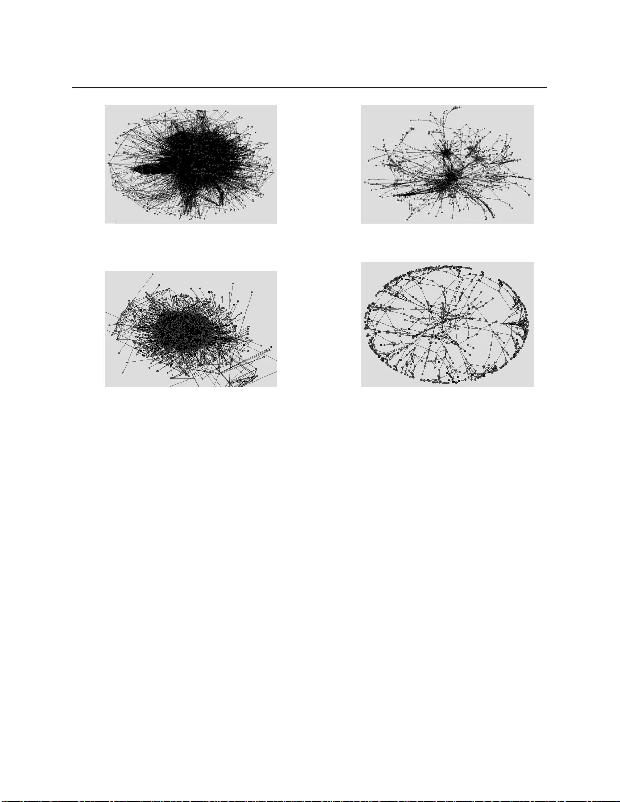
Gaussian Belief Propagation: Theo ry and Application Thesis fo r the degree of DOCTOR of PHILOSOPHY b y Danny Bickson submitted to the sena te of The Hebrew University of Jer usalem 1 st V ersion: Octob er 2 008. 2 nd Revision: May 2009. This w o rk w as ca rried o ut under the sup ervision of Prof. Danny Dolev and Prof. Dahlia Malkhi ii Ackno wledgements I w ould first lik e to thank my advisors , Prof. Danny Dolev a nd Prof. Dahlia Ma lkhi. Danny Dolev enc ouraged me to follo w this interesting resear ch direction, had infinite time to meet and our b rainsto rming sessions where alw a ys valuable and enjo y able. Dahlia M alkhi encouraged me to do a Ph.D., w ork ed with me closely at the first part of my Ph.D., a nd w as alw a ys energetic and inspiring. My tim e as in Intern i n Microsoft Resea rch, Silicon Valley , will never b e forgotten, in the p erio d where my resea rch skills where immensely imp ro v ed. I w ould lik e to thank Prof. Y air W eiss, fo r teaching highly interesting courses and intro ducing me to the graphical mo dels wo rld. Also fo r continuous supp ort in answ ering millions of questions. Prof. Scott Kirkpatrick intro duced me to the wo rld of statistical physics, mainly using the Evergro w p roj ect. It w a s a pleasure w orking with him, sp ecifically w atching his sup erb manage- ment skills which could defeat every o bstacle. In this p roj ect, I’v e also met Prof. Erik Aurell from SICS/KTH and we had numerous interesting discussions ab o ut Gaussians, the b read-and-butter of statistical physics. I am lucky that I had the opp ortunit y to wo rk with Dr. Ori Shental from USCD. Ori intro duced me into the w o rld of information theory and tog ether w e had a fruitful joint resea rch. F urther thanks to Prof. Y uval Shav i tt from T el Aviv univ ersit y , for serving in my Ph.D. com- mittee, and for fruitful discussions. Supp o rt vecto r regress ion w ork w as done when I w as intern in IB M Resea rch Haifa Lab. Thanks to Dr. Elad Y om-T ov and Dr. Oded Margalit for their encouragement and for our enjoy able joint w o rk. The linea r pr ogramming and Kalma n filter w o rk w a s done with the great encouragement of Dr. Gidon Gershinsky from IBM Haif a Reseach Lab. I thank Prof . Andrea Montanari f or sha ring his multiuser detection co de. I w ould like to thank Dr. Misha Chetk ov and Dr. J ason K. Johnson for inviting me to visit Los Alamos National Lab, which resulted in the convergence fix results, reported in this wo rk. F urther encouragement I got from Prof. Stephen Boyd, Stanfo rd Universit y . Finally I would lik e to thank my wife Rav it, fo r her continuous support. iii Abstract The canonical p roblem of solving a system of linea r equations arises in numerous contexts in info rmation theo ry , communication theory , a nd related fields. In this contribution, w e develop a solution based up on Gaussian b elief p ropagation (GaBP) that do es not inv olve direct matrix inversion. The iterative nature of our approach allows fo r a distributed message-passing imple- mentation o f the solution algorithm. In the first pa rt of this thesis, w e a ddress the p rop erties of the Ga B P solver. W e charact erize the rate of conv ergence, enhance its message-passing efficienc y b y intro ducing a b roadcast version, discuss its relation to classical solution metho ds including nu- merical examples. We p resent a new metho d fo r fo rcing the GaBP algorithm to converge to the co rrect solution for a rbitra ry column dep endent matrices. In the second part w e give five applications to illustrate the applicability of the GaBP algo rithm to very l arge computer net w orks: P eer-to-Peer rating, linear detection, distributed computation of supp o rt vecto r regression, efficient computation of Kalman filter and distributed linear p ro- gramming. Using extensive simulations on up to 1,024 CPUs in pa rallel using IBM Bluegene sup ercomputer w e demonstrate the attractiveness and applicabilit y of the GaBP al g o rithm, using real net w o rk top ol o gies with up to millions of no des and hundreds of millions of communication links. W e further relate to several other algorithms and explore their connection to the GaBP algo rithm. iv Contents 1 Intro duction 1 1.1 Material Covered in this Thesis . . . . . . . . . . . . . . . . . . . . . . . . . . 3 1.2 Prelimina ries: Notations and Definitions . . . . . . . . . . . . . . . . . . . . . . 3 1.3 Problem F o rmulation . . . . . . . . . . . . . . . . . . . . . . . . . . . . . . . . 5 P a rt 1: Theo ry 7 2 The GaBP Algorithm 8 2.1 Linea r Algeb ra to I nference . . . . . . . . . . . . . . . . . . . . . . . . . . . . 8 2.2 Belief Propagation . . . . . . . . . . . . . . . . . . . . . . . . . . . . . . . . . 10 2.3 GaBP Algor ithm . . . . . . . . . . . . . . . . . . . . . . . . . . . . . . . . . . 11 2.4 Max-Pro duct Rule . . . . . . . . . . . . . . . . . . . . . . . . . . . . . . . . . 15 2.5 Prop erties . . . . . . . . . . . . . . . . . . . . . . . . . . . . . . . . . . . . . 16 3 GaBP Algorithm Prop erties 17 3.1 Upp er Bound on R ate . . . . . . . . . . . . . . . . . . . . . . . . . . . . . . . 17 3.2 Convergence Acceleration . . . . . . . . . . . . . . . . . . . . . . . . . . . . . 19 3.3 GaBP Broadcast . . . . . . . . . . . . . . . . . . . . . . . . . . . . . . . . . . 19 3.4 The GaBP-Based Solv er a nd Classical Solution Metho ds . . . . . . . . . . . . . . . . . . . . . . . . . . . . . . . . . . . . . . 21 3.4.1 Gaussian Elimination . . . . . . . . . . . . . . . . . . . . . . . . . . . . 21 3.4.2 Iterative Metho ds . . . . . . . . . . . . . . . . . . . . . . . . . . . . . 23 3.4.3 Jacobi Metho d . . . . . . . . . . . . . . . . . . . . . . . . . . . . . . . 24 4 Numerical E x amples 25 4.1 T o y Linea r System . . . . . . . . . . . . . . . . . . . . . . . . . . . . . . . . . 25 4.2 Non PSD Example . . . . . . . . . . . . . . . . . . . . . . . . . . . . . . . . . 2 7 4.3 2D P oisson’s . . . . . . . . . . . . . . . . . . . . . . . . . . . . . . . . . . . . 27 5 Convergence Fix 34 5.1 Problem Setting . . . . . . . . . . . . . . . . . . . . . . . . . . . . . . . . . . 34 5.2 Diagonal Loading . . . . . . . . . . . . . . . . . . . . . . . . . . . . . . . . . 35 5.3 Iterative Co rrection Metho d . . . . . . . . . . . . . . . . . . . . . . . . . . . . 35 v CONTENTS CONTENTS 5.4 Extension to General Linea r Systems . . . . . . . . . . . . . . . . . . . . . . . 37 P a rt 2: Applicati ons 38 6 P eer-to-P eer Rating 39 6.1 F ramew or k . . . . . . . . . . . . . . . . . . . . . . . . . . . . . . . . . . . . . 40 6.2 Quadratic Cost Functions . . . . . . . . . . . . . . . . . . . . . . . . . . . . . 41 6.2.1 P eer-to-P eer Rating . . . . . . . . . . . . . . . . . . . . . . . . . . . . 44 6.2.2 Spatial Ranking . . . . . . . . . . . . . . . . . . . . . . . . . . . . . . 44 6.2.3 P ersonalized P ageRank . . . . . . . . . . . . . . . . . . . . . . . . . . 46 6.2.4 Info rmation Centralit y . . . . . . . . . . . . . . . . . . . . . . . . . . . 46 6.3 Exp erimental Results . . . . . . . . . . . . . . . . . . . . . . . . . . . . . . . . 46 6.3.1 Rating Benchma rk . . . . . . . . . . . . . . . . . . . . . . . . . . . . . 48 7 Linea r Detection 51 7.1 GaBP Extension . . . . . . . . . . . . . . . . . . . . . . . . . . . . . . . . . . 56 7.1.1 Distributed Iterative Computation of the MMSE Detecto r . . . . . . . . 56 7.1.2 Relation to F actor Graph . . . . . . . . . . . . . . . . . . . . . . . . . 57 7.1.3 Convergence Analysis . . . . . . . . . . . . . . . . . . . . . . . . . . . 58 7.2 Applying GaBP Convergence Fix . . . . . . . . . . . . . . . . . . . . . . . . . 59 8 SVR 62 8.1 SVM Classification . . . . . . . . . . . . . . . . . . . . . . . . . . . . . . . . . 62 8.2 KRR Problem . . . . . . . . . . . . . . . . . . . . . . . . . . . . . . . . . . . 64 8.3 Previous App roaches . . . . . . . . . . . . . . . . . . . . . . . . . . . . . . . . 64 8.4 Our novel construction . . . . . . . . . . . . . . . . . . . . . . . . . . . . . . . 66 8.5 Exp erimental Results . . . . . . . . . . . . . . . . . . . . . . . . . . . . . . . . 66 8.6 Discussion . . . . . . . . . . . . . . . . . . . . . . . . . . . . . . . . . . . . . 69 9 Kalman F ilter 71 9.1 Kalman Filter . . . . . . . . . . . . . . . . . . . . . . . . . . . . . . . . . . . 72 9.2 Our Construction . . . . . . . . . . . . . . . . . . . . . . . . . . . . . . . . . . 72 9.3 Gaussian Infor mation Bottleneck . . . . . . . . . . . . . . . . . . . . . . . . . 7 4 9.4 Relation to the Affine-Scaling Algo rithm . . . . . . . . . . . . . . . . . . . . . 77 10 Linear Programming 80 10.1 Standar d Linear Programming . . . . . . . . . . . . . . . . . . . . . . . . . . . 81 10.2 F rom LP to Inference . . . . . . . . . . . . . . . . . . . . . . . . . . . . . . . 82 10.3 Extended Construction . . . . . . . . . . . . . . . . . . . . . . . . . . . . . . . 83 10.3.1 Applications to Interior-P oint Metho ds . . . . . . . . . . . . . . . . . . 8 5 10.4 NUM . . . . . . . . . . . . . . . . . . . . . . . . . . . . . . . . . . . . . . . . 8 6 10.4.1 NUM Problem Fo rmulation . . . . . . . . . . . . . . . . . . . . . . . . 86 10.4.2 Previous Wo rk . . . . . . . . . . . . . . . . . . . . . . . . . . . . . . . 87 vi CONTENTS CONTENTS 10.4.3 Exp erimental Results . . . . . . . . . . . . . . . . . . . . . . . . . . . . 89 11 Relation to Other Algo rithm s 92 11.1 Montanari’s MUD . . . . . . . . . . . . . . . . . . . . . . . . . . . . . . . . . 92 11.2 F rey’s I PP Algo rithm . . . . . . . . . . . . . . . . . . . . . . . . . . . . . . . . 94 11.3 Consensus Propag a tion . . . . . . . . . . . . . . . . . . . . . . . . . . . . . . 96 11.4 Quadratic Min- Sum . . . . . . . . . . . . . . . . . . . . . . . . . . . . . . . . 98 12 App endices 100 12.1 Weis s vs. Johnson . . . . . . . . . . . . . . . . . . . . . . . . . . . . . . . . . 100 12.2 GaBP co de in Matlab . . . . . . . . . . . . . . . . . . . . . . . . . . . . . . . 101 12.2.1 The file gabp.m . . . . . . . . . . . . . . . . . . . . . . . . . . . . . . 101 12.2.2 The file run gabp.m . . . . . . . . . . . . . . . . . . . . . . . . . . . . 103 vii Chapter 1 Intro duction Solving a linea r system of equations Ax = b i s one o f the most fundamental problems in algeb ra, with countles s applications in the mathematical scie nces and enginee ring. In this the sis, w e p rop ose an efficient di stributed iterative algorithm fo r solving systems of linea r equations. The problem of solving a linea r system of equations is describ ed as follo ws. Given an ob- servation vec to r b ∈ R m and the data matrix A ∈ R m × n ( m ≥ n ∈ Z ), a unique solution, x = x ∗ ∈ R n , exists if and only if the data matrix A has full column rank. Assuming a nonsin- gula r matrix A , the system of equations can b e solv ed either directly or in a n iterative manner. Direct matrix inversion metho ds, such as Gaussian elimination (L U factorization, [ 1 ]-Ch. 3) or band Cholesky f a cto rization ( [ 1 ]-Ch. 4), find the solution with a finite numb er of op erations, t ypically , fo r a dense n × n ma trix, of the order of n 3 . The for mer is partic ula rly effective for systems with unstructured dense data ma trices, while the la tter is t ypically used fo r structured dense systems. Iterative metho ds [ 2 ] a re inherently simpler, requiring only additions and multiplications, and have the further advantage that they can exploit the spa rsit y of the matrix A to reduce the computational complexit y as w ell as the algorithmic sto ra g e requireme nts [ 3 ]. By compa rison, for la rge, spa rse and a mo rphous data matrices, the direct methods a re imp ractical due to the need fo r excessive matrix reo rdering op erations. The main drawback of the iterative app roaches is that, under certain conditions, they converge only a symptotically to the exact solution x ∗ [ 2 ]. Thus, there is the risk that they ma y converge slo wly , o r not at all. In p ra ctice, ho wever, it has b een found that they often converge to the exa ct solution or a go o d appro ximation a fter a relatively small numb er of iterations. A p o w erful and efficient iterative a lgo rithm, b elief p ropagation (BP , [ 4 ]), also kno wn as the sum-p ro duct algo rithm, has b een very success fully used to solve, either exactly o r appro xima tely , inference pr oblems in p roba bilistic graphical mo dels [ 5 ]. In this thesis, w e reform ulate the general p roblem o f solving a linea r syst em of algeb raic equations as a p robabilistic inference p roblem on a suitably-defined graph 1 . F urtherm o re, fo r 1 Recently , we have found ou t the wo rk o f Moa l lemi and V an R oy [ 6 ] which dis cusses the connection b etw een the Min-Sum message passing algorithm and solving quadratic programs. Both w orks [ 7 , 6 ] were publi s hed in par allel, and th e algorithms where derived indep endently , using different techniques. In Section 11.4 we discuss 1 CHAPTER 1. INTRODUCTION the first time, a full step-b y-step derivation of the GaBP alg o rithm from the b elief p ropagation algo rithm is provided. As an imp o rtant consequence, w e demonstrate that Gaussian BP (GaBP) p ro v ides an effi- cient, distributed app roach to solving a linea r system that circumvents the p otentially complex op eration of direct matrix inversion. Using the seminal w ork of W eiss and F reeman [ 8 ] and some recent related developments [ 9 , 10 , 6 ], w e address the conv ergence a nd exactness p rop erties of the p rop osed GaBP solver. This thesis is structure d as follo ws Chapter 2 intro duces the GaBP by p roviding a clean step- b y-step derivation of the GaBP algo rithm by substituting g a ussian p roba bilit y into P earl’s b elief p ropagation up date rules. Sta rting from Chapter 3 , we p resent our novel contributions in this do main. Chapter 3 p resents our novel b roadcast version o f GaBP that reduces the numb er o f unique messages on a dense graph from O ( n 2 ) to O ( n ) . This version allo ws for efficient implementation on communication net wo rks that supp ort s b roadcast such as wireless and Ethernet. (Ex ample of an efficient implementation of the broadcast version on top of 1,024 CPUs is rep ort ed in Chapter 8 ). W e investigate the use of acceleration metho ds from linear algebra to b e applied fo r GaB P . We compa re metho dically GaBP algorithm to other linea r iterative metho ds. Chapter 3 further p rov ides theo retical analysis of GaBP convergence rate assuming diagonally dominant inverse cov ariance matrix. This is the first time convergence rate of GaBP is cha racterized. In Chapter 4 w e give numerical examples for ill ustrating the convergence p rop erties of the GaBP algorithm. The GaBP algorithm, lik e the linear i terative metho ds, has sufficient conditions for conver- gence. When those sufficient conditions do not hold, the algo rithm ma y diverge. T o address this problem, Chapter 5 p resents our novel construction fo r fo rcing convergence of the GaBP algo rithm to the corr ect solution, for p ositive definite matrices , as w ell a s for column dep endent non-squa re matrices. W e b elieve that this result is o ne o f the main novelties of this w ork, since it applies not only to the GaBP algorithm but to other li near iterative metho ds as w ell. The second part o f this w o rk is ma inl y concentrated with applications for the GaBP a lg o rithm. The first application we investigate (Chapter 6 ) is the rating of no des in a Pe er-to-P eer net w o rk. W e p rop o se a unify ing family of quadratic cost functions to b e used in P eer-to-P eer ratings. We sho w that our approach is general, since it captures many o f the existing algorithms in the fields o f visual lay o ut, collab orative filtering and Peer-to-P eer rating, among them Kore n’s sp ectral la y out algo rithm, Katz’s metho d, Spatial ranking, Pers onalized PageRank and Information Centralit y . Beside of the theo retical interest in finding common basis of algo rithms that we re not link ed b efo re, we allo w a single efficient implementation fo r computing those va rious rating metho ds, using the GaBP solv er. W e p rov ide simulation results on top of real life top olo gies including the MSN Messenger social net wo rk. In Chapter 7 we consider the pr oblem of linea r detection using a decorre lato r in a co de- division multiple-access (CDMA) system. Through the use of the iterative mess age-passing fo rmulation, w e implement the deco rrelato r detecto r in a distributed manner. This example allo ws us to quantitatively compa re the new GaBP solver with the classical iterative solution the conn e c ti on b et ween th e tw o algorithms, and show they ar e equivalent. 2 CHAPTER 1. INTRODUCTION 1.1. M A TERIAL CO VERED IN T HIS THESIS metho ds that have b een previously investigated in the context of a linea r implementation of CDMA demo dulation [ 11 , 12 , 13 ]. We sho w that the GaBP-based deco rrelato r y ields faster convergence than these conventional methods. W e further extend the appli cability of the GaBP solver to non-squa re column dep endent ma trices. Third a pplication from the field of machine learning is supp ort vecto r regression, describ ed in Chapter 8 . W e sho w how to compute k ernel ridge regression using our GaBP solver. F or demonstrating the applicabili ty of our approach w e used a cluster of IBM BlueGene computers with up to 1,024 CPUs in pa rallel on very large data sets consisting of millions of data p oints. Up to date, this is the la rgest implementation of b elief p ropagation ever p erformed. F ourth application is the efficient distributed calculation of Ka lma n filter, p resent ed in Chapter 9 . W e further p rovide some theore tical results that link the Kalman filter algorithm to the Gaussian info rmation b ottleneck algorithm and the Affine-scaling interio r p oint metho d. Fifth application is the efficient distributed solution of li nea r programming p roblems using GaBP , p rese nted in Chapter 10 . As a case study , w e di scuss the net w o rk utilit y ma ximization p roblem and sho w that our construction ha s a b etter accuracy than previous metho ds, despite the fact it is distributed. W e p rovide a lar ge scale simulation using netw o rks o f hundreds of thousands of no des. Chapter 11 identifies a family of previously proposed al g o rithms, sho wing they are instances of GaBP . This provides the abilit y to apply the vast knowled ge ab out GaBP to those sp ecial cases, fo r example applying sufficient conditions f or convergence as we ll as applying the convergence fix p resent ed in Chapter 5 . 1.1 Material Covered in this Thesis This thesis is div ided into t w o parts. The first part discusses the theor y of Gaussian b elief p ropagation algorit hm and covers the following pap ers: [ 7 , 14 , 15 , 16 , 17 , 18 ]. The second part discusses several a pplications that w ere covered i n the foll owing pap ers: [ 19 , 20 , 21 , 22 , 23 , 24 , 2 5 ]. Belo w w e brie fly outline some other related pap ers that did not fit into the main theme of this thesis. W e have lo ok ed at b elief p ropagation at the using discret e distribution as a basis for va rious distributed algorithms : clustering [ 26 ], data placement [ 27 , 28 ] Peer -to-Pe er streaming media [ 29 ] and wireles s settings [ 30 ]. The other major topic we wo rk ed on is Peer-to-P eer net wo rks, especially content distribution net w orks (CDNs). The Julia content distribution net wo rk is described on [ 31 , 32 ]. A mo dified version of J ulia using net wo rk co ding [ 33 ]. T ulip is a Pe er- to-P eer overla y that enables fa st routing and sea rching [ 34 ]. The eMule p roto col sp ecification is found on [ 35 ]. An implementation of a distributed testb ed on eight Europ ean clusters is found on [ 36 ]. 1.2 Prelimina ries: Notations and Definitions W e shall use the fo ll owing linear-algeb raic notations and definitions. The op erator {· } T stands fo r a vecto r o r matrix transpo se, the matrix I n is an n × n identit y matrix, while the symb ols {·} i 3 1.2. PRELIMI NARIES: NOT A TIONS AND DEFINITIONS CHAPTER 1. INTR ODUCTION and {· } ij denote entries of a vecto r and matrix, respectively . Let M ∈ R n × n b e a real symmetric squa re ma trix a nd A ∈ R m × n b e a real (p ossibly rectangula r) matrix. Let 1 denotes the all ones vecto r. Definition 1 (Pseudoinverse) . The Mo o re-P enrose pseudoinverse ma trix of the matrix A , de- noted by A † , is defined as A † , ( A T A ) − 1 A T . (1.1) Definition 2 (Sp ectral radius) . The sp ectral radius of the matrix M , denoted by ρ ( M ) , is defined to b e the maximum of the absolute values of the eigenvalues of M , i.e. , ρ ( M ) , max 1 ≤ i ≤ s ( | λ i | ) , (1.2) where λ 1 , . . . λ s a re the eigenvalues of the matrix M . Definition 3 (Diagona l dominance) . The matrix M is 1. we akly dia gonally dominant if | M ii | ≥ X j 6 = i | M ij | , ∀ i , (1.3) 2. strictly diagonally dominant if | M ii | > X j 6 = i | M ij | , ∀ i, (1.4) 3. irreducibly diagonally dominant if M is irreducible 2 , and | M ii | ≥ X j 6 = i | M ij | , ∀ i , (1.5) with strict i nequality fo r at least one i . Definition 4 (PSD) . T he matrix M is p ositive semi-definite (PSD) if and only if for all non-zero real vector s z ∈ R n , z T Mz ≥ 0 . (1.6) Definition 5 (Residual) . F o r a real vector x ∈ R n , the residual, r = r ( x ) ∈ R m , of a linear system is r = Ax − b . The standa rd norm of the residual, || r || p ( p = 1 , 2 , . . . , ∞ ) , is a go o d measure of the a ccuracy of a vecto r x as a solution to the linea r system. I n our exp erimental study , the F rob enius no rm ( i.e. , p = 2 ) p er equation is used, 1 m || r || F = 1 m p P m i =1 r 2 i . 2 A ma trix is said to b e reducible if there is a p ermutation matrix P s u c h that PMP T is blo ck upp er triangular. Otherwise, it is irreducible. 4 CHAPTER 1. INTRODUCTION 1.3. PROBLEM F ORMULA TION Definition 6 (Op erator No rm) . Given a ma trix M the op erato r no rm || M | | p is defined as || M | | p , sup x 6 =0 || Mx || p || x || p . Definition 7. The condition numb er, κ , of the matrix M is defined as κ p , || M | | p || M − 1 || p . (1.7) F o r M b eing a no rmal matrix (i.e. , M T M = MM T ), the condition numb er is giv en b y κ = κ 2 =    λ max λ min    , (1.8) where λ max and λ min a re the maxima l and minimal eigenvalues of M , resp ectively . Even though a system is no nsingular it could b e ill-conditioned. I ll-conditioning means that a small p erturbation in the data matrix A , o r the observation vecto r b , causes la rge p erturbations in the solution, x ∗ . This determines the difficult y of solving the p roblem. T he condition numb er is a go o d measure of the ill-conditioning of the matrix. The b etter the conditioning of a matrix the smaller the condition numb er. The condition numb er of a non-invertible (singular) matrix is set a rbitra rily to infinit y . Definition 8 (Graph Laplacian 3 [ 37 ]) . Given a matrix a w eighted matrix A describing a graph with n no des, the graph La placian L is a symmetric matrix defined as follows : L i,j = ( i = j deg ( i ) else − w i,j where deg ( i ) = P j ∈ N ( i ) w j i is the degree of no de i. It can b e further sho wn [ 37 ] that given the Laplacian L , it holds that x T L x = P i j . The set of graph no des N( i ) denotes the set of all the no des neighb o ring the i th no de (excluding no de i ). The set N( i ) \ j excludes the no de j from N( i ) . Using this graph, we can translate the problem of solv ing the linear system fro m the a lgeb ra i c domain to the domain of probabilistic inference, as stated in the f o llo wing theo rem. 8 CHAPTER 2. THE GABP ALGORITHM 2.1. LINEAR ALGEBRA T O INFERENCE Ax = b m Ax − b = 0 m min x ( 1 2 x T Ax − b T x ) m max x ( − 1 2 x T Ax + b T x ) m max x exp( − 1 2 x T Ax + b T x ) Figure 2.1: Schematic outline of the of the p ro of to Propo sition 10 . Prop osition 10. The computation of the solution vecto r x ∗ = A − 1 b is identical to the inf erence of the vecto r of mar ginal means µ , { µ 1 , . . . , µ n } over the graph G with the asso ciated j o int Gaussian probabilit y densit y function p ( x ) ∼ N ( µ , A − 1 ) . Pro of. Another w a y of solving the set of linea r equations Ax − b = 0 is to repr esent it b y using a qua dra tic form q ( x ) , x T Ax / 2 − b T x . As the matrix A is symmetric, the derivative of the quadratic f o rm w.r.t. the vector x is given b y the v ecto r ∂ q /∂ x = Ax − b . Thus equating ∂ q /∂ x = 0 gives the global minimum x ∗ of this conv ex function, which is nothing but the desired solution to Ax = b . Next, one can define the fo ll owing joint Gaussian probabilit y densit y function p ( x ) , Z − 1 exp  − q ( x )  = Z − 1 exp ( − x T Ax / 2 + b T x ) , (2.2) where Z is a distribution no rmalization facto r. Denoting the v ecto r µ , A − 1 b , the Gaussian densit y function can b e rewritten a s p ( x ) = Z − 1 exp ( µ T A µ/ 2) × exp ( − x T Ax / 2 + µ T Ax − µ T A µ/ 2) = ζ − 1 exp  − ( x − µ ) T A ( x − µ ) / 2  = N ( µ , A − 1 ) , (2.3) where the new normalization f acto r ζ , Z exp ( − µ T A µ/ 2) . It f ollo ws that the ta rget solu- tion x ∗ = A − 1 b is equal to µ , A − 1 b , the mean vector of the distribution p ( x ) , as defined ab ove ( 2.2 ). Hence, in orde r to solve the system of linea r equations we need to infer the marginal densities, which must also b e Gaussian, p ( x i ) ∼ N ( µ i = { A − 1 b } i , P − 1 i = { A − 1 } ii ) , where µ i and P i a re the mar ginal mean and inverse variance (sometime s called the p recision), resp ectively . 9 2.2. BELIEF PROP AGA TION CHAPTER 2. THE GABP ALGORITHM Acco rding to Prop o sition 10 , solving a deterministic vector-matrix l i near equation translates to solving a n i nf erence problem in the co rresp onding graph. The move to the p robabilistic doma in calls for the utilization of BP as an efficient inference engine. Rema rk 11. Defining a jointly Gaussian p robabilit y densit y function, i mmediately y ields an im- plicit assumption on the p ositive semi-definitenes s of the precis ion matrix A , in addition to the symmetry assumption. How ever, w e w ould like to stress out that this assumption emerges only fo r exp osition purp oses, so we can use the notion o f ‘Gaussian probabilit y’, but the derivation of the GaBP solver itself do es not use this assumption. See the numerical example of the exact GaBP-based solution of a system with a symmetric, but no t p ositive semi-definite, data matrix A in Section 4.2 . 2.2 Belief P ropagation Belief p ro pa gation (BP) is equivalent to applying P ea rl’s lo cal message-passing algo rithm [ 4 ], o riginally derived for exa ct inference in trees, to a general graph even if it contains cycles (lo ops). BP has b een found to have outstanding empirical success in many applications, e.g. , in deco di ng T urb o co des and low-dens it y pa rit y- check (LDPC) co des. The excellent p erfo rmance of BP in these applications may b e attributed to the spa rsit y of the graphs, which ensures that cycles in the graph are long, and inference ma y b e p erformed as if it w ere a tree. The BP algorithm functions b y passing real- valued messages across edges in the graph and consists of tw o computational rules, namely the ‘sum-product rule’ a nd the ‘product rule’. In contrast to t ypical applications of BP in co ding theo ry [ 38 ], our graphical rep resent ation resembles to a pairwise M ark ov rando m field [ 5 ] with a single t yp e of propagating messages, rather than a f a cto r graph [ 39 ] with t w o different t yp es of messages, o rigina ted from either the v ariable no de o r the facto r no de. Furthe rmo re, in most graphical mo del repre sentations used in the info rmation theor y literature the graph no des a re assigned with discrete values, while in this contribution w e deal with no des co rresp onding to continuous variables. Thus, for a graph G comp osed of p otentials ψ ij and φ i as p reviously defined, the conventional sum-product rule b ecomes an integral-p ro duct rule [ 8 ] and the message m ij ( x j ) , sent from no de i to no de j over their sha red edge on the graph, is given by m ij ( x j ) ∝ Z x i ψ ij ( x i , x j ) φ i ( x i ) Y k ∈ N( i ) \ j m k i ( x i ) dx i . (2.4) The ma rginals are computed (as usual) acco rding to the product rule p ( x i ) = αφ i ( x i ) Y k ∈ N( i ) m k i ( x i ) , (2.5) where the scala r α is a normalization constant. Note that the propagating messages (and the graph p otentials) do not have to describ e val id ( i.e. , no rmalized) densit y probabilit y functions, as long as the inferred marginals do. 10 CHAPTER 2. THE GABP ALGORITHM 2.3. GABP ALGORITHM 2.3 The Gau ssian BP Algor ithm Gaussian BP is a sp ecial case of continuous BP , where the underlying distribution is Gaussian. The GaBP algo rithm w as o riginally intro duced by W eiss et al. [ 8 ]. We iss w o rk do not detail the derivation of the GaBP algorithm. W e b elieve that this derivation is imp o rtant fo r the complete understanding of the GaBP algorithm. T o this end, w e derive the Gaussian B P up da te rules b y substituting Gaussian distributions into the continuous BP up date equations. Given the data ma trix A and the observation vecto r b , one can write explicitly the Gaussian densit y function, p ( x ) ∼ exp( − 1 2 x T Ax + b T x ) , and its co rresponding graph G . Using the graph definition and a certain (arbitra ry) pairwise facto rization of the Gaussian function ( 2.3 ), the edge p otentials (’compatibilit y functions’) and self p otentials (‘evidence’) φ i a re determined to b e ψ ij ( x i , x j ) , exp( − 1 2 x i A ij x j ) , (2.6) φ i ( x i ) , exp  − 1 2 A ii x 2 i + b i x i  , (2.7) respectively . Note that b y completing the square, one can observe that φ i ( x i ) ∝ N ( µ ii = b i / A ii , P − 1 ii = A − 1 ii ) . (2.8) The graph top o logy is specified b y the structure of the matrix A , i.e. the edges set { i, j } includes all non-zero entries of A f or which i > j . Befo re describing the inference a lgo rithm p erfo rmed over the graphical mo del, w e make the elementa ry but very useful observation that the pr o duct of Gaussian densities over a common va riable is, up to a constant facto r, also a Gaussian densit y . Lemma 12. Let f 1 ( x ) and f 2 ( x ) b e the p robabil ity densit y functions of a Gaussian random var i- able with t w o p ossible densities N ( µ 1 , P − 1 1 ) and N ( µ 2 , P − 1 2 ) , resp ectively . T hen their p ro duct, f ( x ) = f 1 ( x ) f 2 ( x ) is, up to a constant facto r, the probabilit y densit y function of a Gaussian random variable with distribution N ( µ , P − 1 ) , where µ = P − 1 ( P 1 µ 1 + P 2 µ 2 ) , (2.9) P − 1 = ( P 1 + P 2 ) − 1 . (2.10) Pro of. T aking the p ro duct of the t w o Gaussian pr obabilit y densit y functions f 1 ( x ) f 2 ( x ) = √ P 1 P 2 2 π exp  −  P 1 ( x − µ 1 ) 2 + P 2 ( x − µ 2 ) 2  / 2  (2.11) and completing the squa re, one gets f 1 ( x ) f 2 ( x ) = C √ P 2 π exp  − P ( x − µ ) 2 / 2  , (2.12) with P , P 1 + P 2 , (2.13) µ , P − 1 ( µ 1 P 1 + µ 2 P 2 ) (2.14) 11 2.3. GABP ALGORITHM CHAPTER 2. T HE GABP ALGORITHM and the scalar constant determined b y C , r P P 1 P 2 exp  1 2  P 1 µ 2 1 ( P − 1 P 1 − 1) + P 2 µ 2 2 ( P − 1 P 2 − 1) + 2 P − 1 P 1 P 2 µ 1 µ 2  . (2.15) Hence, the product of the t wo Gaussian densities is C · N ( µ, P − 1 ) . Figure 2.2 : Belief propagation message flow Fig. 2.2 plots a p ortion of a certain graph, describing the neighb o rho o d of no de i . Each no de (empt y circle) is asso ciated with a va riable and self p o tential φ , which is a function of this va riable, while edges go with the pairwise (symmetric) p o tentials Ψ . Messages a re p ropagating along the edges on b o th directions (only the messages relevant for the computation of m ij a re dra wn in Fig. 2.2 ). Lo oking at the right hand side of the integral-product rule ( 2.4 ), no de i needs to first calculate the product of all incoming messages, except fo r the message coming from no de j . Recall that since p ( x ) is jo intly Gaussian, the factoriz ed self p otentials φ i ( x i ) ∝ N ( µ ii , P − 1 ii ) ( 2.8 ) and similarly all messages m k i ( x i ) ∝ N ( µ k i , P − 1 k i ) a re of Ga ussian fo rm as w ell. As the terms in the product of the incoming messages and the self p otential in the integral- p ro duct rule ( 2.4 ) are all a function of the same variable, x i (asso ciated with the no de i ), then, acco rding to the multiva riate extension of Lemma 12 , N ( µ i \ j , P − 1 i \ j ) ∝ φ i ( x i ) Y k ∈ N( i ) \ j m k i ( x i ) . (2.16) Applying the multivariate version of the product prec ision expr ession in ( 2.10 ), the up date rule fo r the inv erse va riance is giv en b y (over-b races denote the o rigin of each of the terms) P i \ j = φ i ( x i ) z}|{ P ii + X k ∈ N( i ) \ j m ki ( x i ) z}|{ P k i , (2.17) 12 CHAPTER 2. THE GABP ALGORITHM 2.3. GABP ALGORITHM where P ii , A ii is the inverse variance a-prio ri asso ciated with no de i , via the pre cision of φ i ( x i ) , and P k i a re the inverse va riances of the messages m k i ( x i ) . Similarly using ( 2.9 ) for the multiva riate case, we can calculate the mean µ i \ j = P − 1 i \ j  φ i ( x i ) z }| { P ii µ ii + X k ∈ N( i ) \ j m ki ( x i ) z }| { P k i µ k i  , (2.18) where µ ii , b i / A ii is the mean of the self p o tential and µ k i a re the means of the incoming messages. Next, we calculate the remaining terms of the message m ij ( x j ) , including the integration over x i . m ij ( x j ) ∝ Z x i ψ ij ( x i , x j ) φ i ( x i ) Y k ∈ N( i ) \ j m k i ( x i ) dx i (2.19) ∝ Z x i ψ ij ( x i ,x j ) z }| { exp ( − x i A ij x j ) φ i ( x i ) Q k ∈ N( i ) \ j m ki ( x i ) z }| { exp ( − P i \ j ( x 2 i / 2 − µ i \ j x i )) dx i (2.20) = Z x i exp (( − P i \ j x 2 i / 2) + ( P i \ j µ i \ j − A ij x j ) x i ) dx i (2.21) ∝ exp (( P i \ j µ i \ j − A ij x j ) 2 / (2 P i \ j )) (2.22) ∝ N ( µ ij = − P − 1 ij A ij µ i \ j , P − 1 ij = − A − 2 ij P − 1 i \ j ) , (2.23) where the exp onent ( 2.22 ) is obtained b y using the Gaussian integral ( 2.24 ): Z ∞ −∞ exp ( − ax 2 + bx ) dx = p π /a ex p ( b 2 / 4 a ) , (2.24) w e find that the messages m ij ( x j ) ar e p ro p o rtional to no rmal distribution with p recision and mean P ij = − A 2 ij P − 1 i \ j , (2.25) µ ij = − P − 1 ij A ij µ i \ j . (2.26) These t w o scalars rep resent the messages propagated in the Ga ussian BP-based algorithm. Finally , computing the p ro duct rule ( 2.5 ) is similar to the calculation of the pr evious p ro d- uct ( 2.16 ) a nd the resulting mean ( 2.18 ) and p recision ( 2.17 ), but including all incoming mes- sages. The marginals a re inferred by no rmalizing the result of this pro duct. Thus, the ma rginals a re found to b e Gaussian probabilit y densit y functions N ( µ i , P − 1 i ) with pre cision and mean P i = φ i ( x i ) z}|{ P ii + X k ∈ N( i ) m ki ( x i ) z}|{ P k i , (2.27) µ i = P − 1 i \ j  φ i ( x i ) z }| { P ii µ ii + X k ∈ N( i ) m ki ( x i ) z }| { P k i µ k i  , (2.28) 13 2.3. GABP ALGORITHM CHAPTER 2. T HE GABP ALGORITHM respectively . The derivation of the GaBP-based solver algorith m is concluded by simply substi- tuting the explicit derived expres sions of P i \ j ( 2.17 ) into P ij ( 2.25 ), µ i \ j ( 2.18 ) and P ij ( 2.25 ) into µ ij ( 2.26 ) and P i \ j ( 2.17 ) into µ i ( 2.28 ). The message passing in the GaB P solver can b e p erformed subject to any scheduling. W e refer to tw o conventional messages up dating rules: parallel (flo o ding or synchronous) and serial (sequential, asynchronous) scheduling. I n the pa rallel scheme, messages a re stored in tw o data structures : messages from the p revious iteration round, and messages f ro m the current round. Thus, incoming messages do not affect the result of the computation in the current round, since it is done on messages that w ere received in the previous iteration round. Unlike this, in the serial scheme, there is only one data structure, so incoming messages in this round, change the result of the computation. In a sense it is exactly lik e the difference b et w een the Jacobi and Gauss-Seidel algo rithms, to b e discussed in the following. Some in-depth discussions ab out parallel vs. serial scheduling in the BP context (the discrete case) can b e found in the w o rk of Elidan et al. [ 40 ]. Algo rithm 1. 1. Init ialize: X Set the neighborhood N ( i ) to includ e ∀ k 6 = i ∃ A k i 6 = 0 . X Set the scalar fixes P ii = A ii and µ ii = b i / A ii , ∀ i . X Set the initial N( i ) ∋ k → i scalar messages P k i = 0 and µ k i = 0 . X Set a convergence threshold ǫ . 2. Iter ate: X Propagate the N( i ) ∋ k → i messages P k i and µ k i , ∀ i (unde r certain scheduling) . X Compute the N( j ) ∋ i → j scalar mess ages P ij = − A 2 ij /  P ii + P k ∈ N( i ) \ j P k i  , µ ij =  P ii µ ii + P k ∈ N( i ) \ j P k i µ k i  / A ij . 3. Chec k: X If the messages P ij and µ ij did not converge (w.r.t. ǫ ), return to Step 2. X Else, continue to Step 4. 4. Infe r: X Compute the marginal means µ i =  P ii µ ii + P k ∈ N( i ) P k i µ k i  /  P ii + P k ∈ N( i ) P k i  , ∀ i . ( X Optionally compute the marginal precisions P i = P ii + P k ∈ N( i ) P k i ) 5. Solv e: X Find the solution x ∗ i = µ i , ∀ i . 14 CHAPTER 2. THE GABP ALGORITHM 2.4. M AX-PRODUCT RULE 2.4 Max-Pro duct Rule A w ell- kno wn alternative version to the sum-p ro duct BP is the max-product (a.k.a. min-sum) algo rithm [ 41 ]. In this va riant of BP , maximization op eration is p erfo rmed rather than ma rginal- ization, i.e. , variables a re eliminated b y taking maxima instead of sums. Fo r T rellis trees ( e.g. , graphically rep resenting convolutional co des or ISI channels), the conventional sum-pr o duct BP algo rithm b o il s dow n to p erforming the BCJR a lgo rithm [ 42 ], resulting in the most p robable sym- b ol, while its max- p roduct counterpa rt is equivalent to the Viterbi algor ithm [ 43 ], thus inferring the most probable sequence of symb ols [ 39 ]. In order to derive the max-pro duct v ersion of the p rop osed GaBP solver, the integral (sum)- p ro duct rule ( 2.4 ) is replaced b y a new rule m ij ( x j ) ∝ arg max x i ψ ij ( x i , x j ) φ i ( x i ) Y k ∈ N( i ) \ j m k i ( x i ) dx i . (2.29) Computing m ij ( x j ) acco rding to this max-product rule, o ne gets m ij ( x j ) ∝ arg max x i ψ ij ( x i , x j ) φ i ( x i ) Y k ∈ N( i ) \ j m k i ( x i ) (2.30) ∝ a rg max x i ψ ij ( x i ,x j ) z }| { exp ( − x i A ij x j ) φ i ( x i ) Q k ∈ N( i ) \ j m ki ( x i ) z }| { exp ( − P i \ j ( x 2 i / 2 − µ i \ j x i )) (2.31) = arg max x i exp (( − P i \ j x 2 i / 2) + ( P i \ j µ i \ j − A ij x j ) x i ) . (2.32) Hence, x max i , the value o f x i maximizing the p ro duct ψ ij ( x i , x j ) φ i ( x i ) Q k ∈ N( i ) \ j m k i ( x i ) is given b y equating its derivative w.r.t. x i to zero, yielding x max i = P i \ j µ i \ j − A ij x j P i \ j . (2.33) Substituting x max i back into the p ro duct, w e get m ij ( x j ) ∝ exp (( P i \ j µ i \ j − A ij x j ) 2 / (2 P i \ j )) (2.34) ∝ N ( µ ij = − P − 1 ij A ij µ i \ j , P − 1 ij = − A − 2 ij P i \ j ) , (2.35) which is identical to the result obtained when eliminating x i via integration ( 2.23 ). m ij ( x j ) ∝ N ( µ ij = − P − 1 ij A ij µ i \ j , P − 1 ij = − A − 2 ij P i \ j ) , (2.36) which is identical to the messages derived for the sum-p ro duct case ( 2.25 )-( 2.26 ). Thus interest- ingly , as opp osed to ordina ry (discrete) BP , the following p rop erty of the GaB P solver emerges. Co rolla ry 13. The max-p ro duct ( 2.29 ) and sum-product ( 2.4 ) v ersions o f the GaBP solver a re identical. 15 2.5. PROPERTIES CHAPTER 2. THE GABP ALGORITHM 2.5 Convergence and Exactness In o rdinary BP , convergence does not entail exactness of the inferred p roba bilities, unless the graph has no cycles. Luckily , this is not the case fo r the GaBP solver. Its underlying Gaussian nature yields a direct connection b et w een convergence a nd ex a ct inference. M oreover, in contrast to BP the convergence of Ga B P is not limited for tree or sparse graphs and can o ccur even for dense (fully- connected) graphs, adhering to certain rules discussed in the following. W e can use results from the literature on p robabilistic inference in graphical mo dels [ 8 , 9 , 10 ] to determine the convergence and exactness p rop erties of the GaBP-based solver. T he fo l lowing t w o theo rems establish sufficient conditions under which GaBP is guaranteed to converge to the exact marginal means. Theo rem 14 . [ 8 , Claim 4] I f the matrix A is strictly diagonally dominant, then GaBP conv erges and the marginal means converge to the true means. This sufficient condition w as recently relaxed to include a wider group of matrices. Theo rem 15 . [ 9 , Prop osition 2] If the sp ectral ra dius of the matrix A satisfies ρ ( | I n − A | ) < 1 , (2.37) then GaBP converges and the ma rginal means converge to the true means. (The assumption here is that the matrix A is first no rmalized b y multiplying with D − 1 / 2 AD − 1 / 2 , where D = diag ( A ) .) A third and w eak er sufficient convergence condition (relative to Theo rem 15 ) which cha ra c- terizes the convergence of the variances is given in [ 6 , Theo rem 2]: F or each ro w in the matrix A , if A 2 ii > Σ j 6 = i A 2 ij then the va riances conv erge. Rega rding the means, additional condition related to Theorem 15 is g i v en. There a re many examples of linea r systems that v io late these conditions, for which Ga BP converges to the exact means. In pa rticula r, if the graph co rresponding to the system is acyclic ( i.e. , a tree), GaBP yields the exact ma rgi na l means (and variances [ 8 ]), rega rdless of the value of the sp ectral ra di us of the matrix [ 8 ]. In contrast to conventional iterative metho ds derived from linea r algebra, understanding the conditions fo r exact convergence remain intriguing op en p roblems. 16 Chapter 3 GaBP Algo rithm Prop erties Sta rting this chapter, w e pr esent our novel contributions in this GaBP domain. W e provide a theo retic al a nalysis of GaBP convergence rate assuming diag onally dominant inverse covariance matrix. This i s the first time conv ergence rate of GaBP is characte rized. Chapter 3 further p resent s our nov el b roadcast version of GaBP , which reduc es the numb er of unique mes sages on a dense graph from O ( n 2 ) to O ( n ) . This v ersion allow s fo r efficient implementation on communication netw o rks that supp o rts broadcast such as wireless and Ethernet. (Example of an efficient implementation of the broadcast version on top of 1,024 CPUs is rep o rted in Chapter 8 ). W e investigate the use of a cceleration metho ds from linea r algebra to b e applied fo r GaBP and compa re metho dically GaBP algorit hm to other linea r iterative metho ds. 3.1 Upp er Bound on Convergence Rate In this section w e give a n upp er b ound on convergence ra te of the GaB P algorithm . As fa r as we kno w this is the first theore tical result b ounding the convergence sp eed of the GaBP algorithm. Our upp er b ound is based on the w o rk of Weis s et al. [ 44 , Claim 4], which p roves the co rrectn ess of the mean computation. W eiss uses the pai rwise p otentials form 1 , where p ( x ) ∝ Π i,j ψ ij ( x i , x j )Π i ψ i ( x i ) , ψ i,j ( x i , x j ) , exp( − 1 2 [ x i x j ] T V ij [ x i x j ]) . ψ i,i ( x i ) , exp( − 1 2 x T i V ii x i ) . W e further assume scalar va riables. Denote the entries of the inverse pairwise cova riance matrix V ij and the inverse cova riance matrix V ii as: V ij ≡  ˜ a ij ˜ b ij ˜ b j i ˜ c ij  , V ii = ( ˜ a ii ) . 1 W eiss assumes variables with zero means. T he mean value do es n o t affect convergence spee d . 17 3.1. UPPER BOUND ON RA TE CHAPTER 3. GABP ALGORIT HM PROPERTIES Assuming the optimal solution is x ∗ , fo r a desired accuracy ǫ || b || ∞ where || b | | ∞ ≡ max i | b i | , and b is the shift vecto r, [ 44 , Claim 4] proves that the GaBP algorithm converges to an accuracy of | x ∗ − x t | < ǫ || b || ∞ after at most t = ⌈ log( ǫ ) / log ( β ) ⌉ rounds, where β = max ij | ˜ b ij / ˜ c ij | . The problem with applying Weiss ’ result directly to our mo del is that we a re w orking with different parameteriz ations. We use the info rmation form p ( x ) ∝ exp( − 1 2 x T Ax + b T x ) . The decomp osition of the matrix A into pairwise p otentials is not unique. I n o rder to use We iss’ result, w e p ropo se such a decomp osition. Any decompo sition from the i nf ormation form to the pairwise p otentials form should b e subject to the follo wing constraints [ 44 ] P airwise form z}|{ ˜ b ij = Info rmation for m z}|{ a ij , which means that the inv erse cova riance in the pairwise mo del should b e equivalent to inv erse cova riance in the inf o rmation fo rm. P airwise fo rm z }| { ˜ a ii + X j ∈ N ( i ) ˜ c ij = Info rmation for m z}|{ a ii . The second constraints sa ys that the sum of no de i ’s inverse va riance (in b oth the self p otentials and edge p otentials) should b e identical to the inverse va riance in the info rmation fo rm. W e propo se to initialize the pairwise p otentials as f ollo wing. Assuming the matrix A is diagonally dominant, w e define ε i to b e the non negative gap ε i , | a ii | − X j ∈ N ( i ) | a ij | > 0 , and the following decomp osition ˜ b ij = a ij , ˜ a ij = c ij + ε i / | N ( i ) | , where | N ( i ) | is the numb er of graph neighbors of no de i . Follo wing W eiss, w e define γ to b e γ = max i,j | ˜ b ij | | ˜ c ij | = max i,j | a ij | | a ij | + ε i / | N ( i ) | = max i,j 1 1 + ( ε i ) / ( | a ij || N ( i ) | ) < 1 . In total, w e get that for a desired accuracy of ǫ || b || ∞ w e need to i terate fo r t = ⌈ log( ǫ ) / log ( γ ) ⌉ rounds. Note that this is an upp er b ound and in p ra ctice w e indeed have observed a much faster convergence rate. The computation of the paramete r γ can b e easily do ne in a distributed manner: Each no de lo cally compute s ε i , and γ i = max j 1 / (1 + | a ij | ε i / N ( i )) . Finally , one maximum operation is p erfo rmed globally , γ = max i γ i . 18 CHAPTER 3. GABP ALGORITHM PROPERTIES 3.2. CONVERGENC E A CCELERA TION 3.2 Convergence Acceler ation F urther sp eed-up of GaBP can b e achieved by adapting kno wn acceleration techniques from linear algeb ra, such Aitk en’s metho d and Steffensen’s iterations [ 45 ]. Consider a sequence { x n } where n is the iteration number, and x is the marginal p robabilit y computed b y GaBP . F urther assume that { x n } linea rly converge to the limit ˆ x , and x n 6 = ˆ x fo r n ≥ 0 . Acco rding to Aitk en’s method, if there exists a real numb er a such that | a | < 1 and lim n →∞ ( x n − ˆ x ) / ( x n − 1 − ˆ x ) = a , then the sequence { y n } defined b y y n = x n − ( x n +1 − x n ) 2 x n +2 − 2 x n +1 + x n converges to ˆ x faster than { x n } in the sense that lim n →∞ | ( ˆ x − y n ) / ( ˆ x − x n ) | = 0 . Aitk en’s metho d can b e view ed as a generalization of over-relaxation, since one uses values from three, rather than t w o, consecutive i teration rounds. This metho d can b e easily implemente d in GaBP as every no de computes v alues based only on its o wn histo ry . Steffensen’s iterations inco rp o rate Aitk en’s metho d. Starting with x n , t wo iterations ar e run to get x n +1 and x n +2 . Next, Aitk en’s method is used to compute y n , this value replaces the o riginal x n , and GaBP is executed again to get a new value of x n +1 . This pr o cess is rep eated iteratively until convergence. We rema rk that, al thoug h the convergence rate is imp roved with these enhanced algo rithms, the region of convergence of the acce lerated GaB P solver remains unchanged. Chapter 4 gives numerical examples to illustrate the p rop osed acceleration metho d p erfo rmance. 3.3 GaBP Broadc ast V a riant F o r a dense ma trix A each no de out o f the n no des sends a unique message to every other no de on the fully- connected graph. This recip e results in a total of n 2 messages p er i teration round. The computational complexit y of the GaBP solver as describ ed in Algo rithm 1 f or a dense linea r system, in terms of op erations (multiplications and additions) p er iteration round. is show n in T able 3.1 . In this case, the total numb er of required op erations p er iteration i s O ( n 3 ) . This numb er is obtained by evaluating the numb er of op erations required to generate a message multiplied b y the numb er of messages. B ased on the summation exp ressions fo r the p ro pa gating messages P ij and µ ij , it is easily seen that it tak es O ( n ) op erations to compute such a message. In the dense case, the graph is fully- connecte d resulting in O ( n 2 ) propagating messages. In order to estimate the total numb er of op erations required f o r the GaBP a lgo rithm to solve the linea r system, w e have to evaluate the numb er of iterations required for convergence. It is kno wn [ 46 ] that the numb er of iterations required fo r a n iterative solution metho d is O ( f ( κ )) , where f ( κ ) is a function of the condition numb er of the data matrix A . Hence the tota l complexit y of the GaBP solv er can b e exp resse d by O ( n 3 ) × O ( f ( κ )) . The analytical evaluation of the convergence rate function f ( κ ) is a challenging op en p roblem. How ever, it can b e upp er b ounded b y f ( κ ) < κ . F urthermo re, ba sed on our experimental study , describ ed in Section 4 , w e can conclude that f ( κ ) ≤ √ κ . T his is b ecause t y pically the GaBP algorith m converges f aster than 19 3.3. GABP BROA DCAST CHAPTER 3. GABP ALGORIT HM PROPERTIES Algo rithm Op erations p er msg msgs T otal op erations p er iteration Naive GaBP (Algo rithm 1 ) O ( n ) O ( n 2 ) O ( n 3 ) Broadcast GaBP (Algo rithm 2 ) O ( n ) O ( n ) O ( n 2 ) T able 3.1: Computational complexity of the GaBP solver for dense n × n matrix A . the SOR algorithm. An upp er b ound on the numb er of iterations of the SOR algorithm is √ κ. Thus, the total complexit y of the GaBP solver in this case is O ( n 3 ) × O ( √ κ ) . F o r well- conditioned (as opp osed to ill-conditioned) data matrices the condition numb er is O (1) . Thus, fo r w ell-conditioned linea r systems the total complexit y is O ( n 3 ) , i.e. , the complexit y is cubic, the same order of magnitude as fo r direct solution metho ds, lik e Gaussian elimination. A t first sight, this result may be considered disapp ointing, with no complexity gain w.r.t. direct matrix inversion. Luckily , the GaBP implementation as describ ed in Algorit hm 1 is a naive one, thus termed naive GaBP . In this implementation w e did not tak e into account the co rrelation b et w een the different messages transmitted from a certain no de i . T hese messages, computed b y summation, are distinct from one another in o nly t w o summation terms. Instead of sending a message comp osed of the pair of µ ij and P ij , a no de can b roadcast the aggregated sums ˜ P i = P ii + X k ∈ N( i ) P k i , (3.1) ˜ µ i = ˜ P − 1 i ( P ii µ ii + X k ∈ N( i ) P k i µ k i ) . (3.2) Consequently , each no de can retrieve lo cally the P i \ j ( 2.17 ) and µ i \ j ( 2.18 ) from the sums b y means of a subtraction P i \ j = ˜ P i − P j i , (3.3) µ i \ j = ˜ µ i − P − 1 i \ j P j i µ j i . (3.4) The rest of the algo rithm remains the same. On dense graphs, the b roadcast version sends O ( n ) messages p er round, instead of O ( n 2 ) messages in the GaBP algorit hm. This construction is t ypically useful when implementing the GaBP algorithm in communication netw o rks that supp ort b roadcast (for example Ethernet and wireless netw o rks), where the messages are sent in b roadcast anyw a y . See fo r example [ 47 , 48 ]. Chapter 8 b rings an example of la rge scale implementation of our b roadcast v a riant using 1,024 CPUs. 20 CHAPTER 3. GABP ALGORITHM PROPERTIES 3.4. THE GABP-B ASED SOL VER AND CLASSICAL SOLUTI ON METHODS Algo rithm 2. 1. Init ialize: X Set the neighborhood N( i ) to include ∀ k 6 = i ∃ A k i 6 = 0 . X Set the scalar fixes P ii = A ii and µ ii = b i / A ii , ∀ i . X Set the initial i → N( i ) broadc ast messages ˜ P i = 0 and ˜ µ i = 0 . X Set the initial N( i ) ∋ k → i internal scalars P k i = 0 and µ k i = 0 . X Set a convergence thres hold ǫ . 2. Iter ate: X Broadcast the aggre gated sum messages ˜ P i = P ii + P k ∈ N( i ) P k i , ˜ µ i = ˜ P i − 1 ( P ii µ ii + P k ∈ N( i ) P k i µ k i ) , ∀ i (under certain schedulin g) . X Compute the N( j ) ∋ i → j interna l scalars P ij = − A 2 ij / ( ˜ P i − P j i ) , µ ij = ( ˜ P i ˜ µ i − P j i µ j i ) / A ij . 3. Chec k: X If the internal scalars P ij and µ ij did not converge (w.r.t. ǫ ), return to Step 2. X Else, continue to Step 4. 4. Infe r: X Compute the marginal means µ i =  P ii µ ii + P k ∈ N( i ) P k i µ k i  /  P ii + P k ∈ N( i ) P k i  = ˜ µ i , ∀ i . ( X Optionally compute the marginal precisions P i = P ii + P k ∈ N( i ) P k i = ˜ P i ) 5. Solv e: X Find the solution x ∗ i = µ i , ∀ i . 3.4 The GaBP-Bas ed Solver and Classical S olution Metho ds 3.4.1 Gaussian Elimina ti o n Prop osition 16. The GaBP-based solver (Algo rithm 1 ) for a system of linea r equations rep re- sented by a tree graph is identical to the reno wned Gaussian elimination algo rithm (a.k.a. LU facto rization, [ 46 ]). Pro of. Consider a set of n linea r equations with n unkno wn variables , a unique solution and a tree graph rep resentation. We aim at computing the unkno wn v a riable asso ciated with the ro ot no de. Wi thout loss of g enerality as the tree can b e drawn with any of the o ther no des b eing its 21 3.4. THE GABP-BASED SOL VER AND CLASSICAL SOLUTI O N METHODS CHAPTER 3. GABP ALGORIT HM PROPERTIES ro ot. Let us enumerate the no des in a n ascending o rder from the ro ot to the l eav es (see, e.g., Fig. 3.1 ). 1 2 3 4 5 A 12 A 13 A 24 A 25 Figure 3.1: Example top o logy of a tree with 5 no des As in a tree, each child no de ( i.e. , all no des but the ro ot) ha s only one pa rent no de a nd based on the top- do wn o rdering, it can b e easily observed that the tree graph’s corre sp onding data matrix A must hav e one a nd only one non-zero entry in the upp er triangula r p ortion of its columns. Moreover, fo r a leaf no de this upp er triangular entry is the only non-zero off-diago nal entry in the whole column. See, fo r example, the data matrix asso ciated with the tree graph depicted in Fig 3.1       A 11 A 12 A 13 0 0 A 12 A 22 0 A 24 A 25 A 13 0 A 33 0 0 0 A 24 0 A 44 0 0 A 25 0 0 A 55       , (3.5) where the non- zero upp er triangula r entries are in b o ld and among these the entries co rresponding to leaves are underlined. No w, acco rding to GE w e w o uld lik e to lo wer triangulate the matrix A . T his is done b y eliminating these entries from the leav es to the ro ot. Let l b e a leaf no de, i b e its pa rent and j b e its pa rent ( l ’th no de grandparent ). Then, the l ’th ro w is multiplied by − A li / A ll and added to the i ’th ro w. in this w a y the A li entry is b eing eliminated. How ever, this elimination, transforms the i ’th diag o nal entry to b e A ii → A ii − A 2 li / A ll , o r fo r multiple leaves connected to the same pa rent A ii → A ii − P l ∈ N( i ) A 2 li / A ll . In our exa mple,       A 11 A 12 0 0 0 A 12 A 22 − A 2 13 / A 33 − A 2 24 / A 44 − A 2 25 / A 55 0 0 0 A 13 0 A 33 0 0 0 A 24 0 A 44 0 0 A 25 0 0 A 55       . (3.6) Thus, in a simila r manner, eliminating the pa rent i yields the multiplication of the j ’th diagonal term b y − A 2 ij / ( A ii − P l ∈ N( i ) A 2 li / A ll ) . Recalling that P ii = A ii , we see that the last exp ress ion 22 CHAPTER 3. GABP ALGORITHM PROPERTIES 3.4. THE GABP-B ASED SOL VER AND CLASSICAL SOLUTI ON METHODS is identical to the up date rule of P ij in GaBP . Again, in our example       B 0 0 0 0 0 C 0 0 0 A 13 0 A 33 0 0 0 A 24 0 A 44 0 0 A 25 0 0 A 55       , (3.7) where B = A 11 − A 2 12 / ( A 22 − A 2 13 / A 33 − A 2 24 / A 44 − A 2 25 / A 55 ) , C = A 22 − A 2 13 / A 33 − A 2 24 / A 44 − A 2 25 / A 55 . No w the matrix is fully lo w er triangulated. T o put differently in terms of GaBP , the P ij messages a re subtracted from the diagonal P ii terms to triangulate the data matrix of the tree. P erfo rming the same ro w op erations on the right hand side column vecto r b , it can b e easily seen that w e equivalently get that the o utcome of the ro w op erations is identical to the GaB P solver’s µ ij up date rule. These up dadtes/ro w op erations can b e repeated, in the general case, until the matrix is low er triangulated. No w, in order to compute the value of the unknow n variable asso ciated with the ro ot no de, all w e have to do is divide the first diagonal term b y the transfo rmed value of b 1 , which is identical to the infer stage in the GaBP solver (note that by definition all the no des connected to the ro ot a re its children, as it do es not have pa rent no de). In the example x ∗ 1 = A 11 − A 2 12 / ( A 22 − A 2 13 / A 33 − A 2 24 / A 44 − A 2 25 / A 55 ) b 11 − A 12 / ( b 22 − A 13 / A 33 − A 24 / A 44 − A 25 / A 55 ) . (3.8) Note that the ro ws co rrespo nding to leaves remain unchanged. T o conclude, in the tree graph case, the ‘iterative’ stage (stage 2 on algorithm 1 ) of the GaBP solv er a ctually p erform s lo w er triangula tion o f the matrix, while the ‘infer’ stage (stage 4) reducers to what is known as fo rw a rd substitution. Evidently , using an opp osite o rdering, one can get the complementa ry upp er triangulation and back substitution, resp ectively . It is imp o rtant to note, that based on this proposition, the GaBP solver can b e view ed as GE run over an unwrapp ed version ( i.e. , a computation tree as defined in [ 8 ]) of a general lo opy graph. 3.4.2 Iterative Metho ds Iterative metho ds that can b e express ed in the simple form x ( t ) = Bx ( t − 1) + c , (3.9) where neither the iteration matrix B n o r the vecto r c dep end up o n the iteration numb er t , a re called stationa ry iterative metho ds. In the following, we discuss three main stationa ry iterative metho ds: the Ja cobi metho d, the Gauss-Seidel (GS) metho d and the successive ov errelaxation (SOR) metho d. The GaBP-based solver, in the g eneral case, ca n not b e written in this form, thus can not b e catego rized as a stationa ry iterative metho d. Prop osition 17. [ 46 ] Assuming I − B is invertible, then the iteration 3.9 converges (for any initial guess, x (0) ). 23 3.4. THE GABP-BASED SOL VER AND CLASSICAL SOLUTI O N METHODS CHAPTER 3. GABP ALGORIT HM PROPERTIES 3.4.3 Jacobi Metho d The Jacobi metho d (Gauss, 1823, and Jacobi 184 5, [ 2 ]), a.k.a. the simultaneous iteration metho d, is the oldest iterative metho d fo r solving a squa re li near system of equations A x = b . The metho d assumes that ∀ i A ii 6 = 0 . I t’s complexity is O ( n 2 ) p er iteration. There a re tw o kno w sufficient convergence conditions fo r the Ja cobi metho d. The first condition holds when the matrix A is strictly o r irreducibly diagonally dominant. The second condition holds when ρ ( D − 1 ( L + U )) < 1 . Where D = diag ( A ) , L , U are upp er and low er triangula r matrices of A . Prop osition 18. The Ga BP-based solver (Algorithm 1 ) 1. with inverse va riance messages set to zero, i.e. , P ij = 0 , i ∈ N ( j ) , ∀ j ; 2. incorporating the message received from no de j when computing the message to b e sent from no de i to no de j , i.e. replacing k ∈ N ( i ) \ j with k ∈ N ( i ) , is identical to the Jacobi i terative metho d. Pro of. Setting the p recisions to zero, w e get in co rresp ondence to the ab ove derivation, P i \ j = P ii = A ii , (3.10) P ij µ ij = − A ij µ i \ j , (3.11) µ i = A − 1 ii ( b i − X k ∈ N( i ) A k i µ k \ i ) . (3.12) Note that the inverse relation b etw een P ij and P i \ j ( 2.25 ) is no longer valid in this case. No w, w e rewrite the mean µ i \ j ( 2.18 ) without excluding the information fro m no de j , µ i \ j = A − 1 ii ( b i − X k ∈ N( i ) A k i µ k \ i ) . (3.13) Note that µ i \ j = µ i , hence the inferred ma rginal mean µ i ( 3.12 ) can b e rewritte n as µ i = A − 1 ii ( b i − X k 6 = i A k i µ k ) , (3.14) where the exp ression f o r all neighb ors of no de i is replaced b y the redundant, y et identical, exp ression k 6 = i . This fixed-p oint iteration is identical to the renow ned Jacobi metho d, concluding the p ro of. The fact that J acobi iterations can be obtained as a special case of the GaBP solver further indicates the richness of the proposed algo rithm. 24 Chapter 4 Numerical Examples In this chapter w e report exp erimental study of three numerical examples: toy l inear system, 2D P oisson equation a nd symmetric non-PSD matrix. I n all examples, but the P oisson’s equation 4.8 , b is assumed to b e an m - length all-ones observation vecto r. Fo r fairness in compa rison, the initial guess in all exp eriments, for the various solution metho ds u nder investigation, is tak en to b e the same and is a rbitra rily set to b e equal to the value of the v ecto r b . The stopping criterion in all exp eriments determines that for all p ropagating messages (in the context the GaBP solver) o r all n tentative solutions (in the context of the compa red iterative metho ds) the absolute va lue of the difference should b e less than ǫ ≤ 10 − 6 . As fo r terminology , in the following p erfo rming GaBP with parallel (flo o ding o r synchronous) message scheduling is termed ‘par allel GaBP’, while GaBP with serial (sequential or asynchronous) message scheduling is termed ‘serial Ga BP’. 4.1 Numerical Ex ample: T o y Linea r System: 3 × 3 Equa- tions Consider the follo wing 3 × 3 linea r system   A xx = 1 A xy = − 2 A xz = 3 A y x = − 2 A y y = 1 A y z = 0 A z x = 3 A z y = 0 A z z = 1   | {z } A   x y z   | {z } x =   − 6 0 2   | {z } b . (4.1) W e would like to find the solution to this system, x ∗ = { x ∗ , y ∗ , z ∗ } T . Inv erting the data ma trix A , w e directly solve   x ∗ y ∗ z ∗   | {z } x ∗ =   − 1 / 12 − 1 / 6 1 / 4 − 1 / 6 2 / 3 1 / 2 1 / 4 1 / 2 1 / 4   | {z } A − 1   − 6 0 2   | {z } b =   1 2 − 1   . (4.2) 25 4.1. TOY LINEAR SYSTEM CHAPTER 4. NUMERICAL EXAMPLES Alternatively , w e can no w run the GaBP solver. Fig. 4.1 displa y s the graph, co rresponding to the data matrix A , and the message-passing flo w. As A y z = A z y = 0 , this gra ph is a cycle-free tree, thus Ga BP is gua ranteed to converge in a finite numb er of rounds. As demonstrated in the follo wing, in this example GaBP converges only in t w o rounds, which equals the tree’s dia meter. Each propagating message, m ij , is described b y tw o scala rs µ ij and P ij , standing for the mean and prec ision of this distribution. The evolution of the propagating means a nd p recisions , until convergence, is describ ed in T able 4.1 , where the notation t = 0 , 1 , 2 , 3 denotes the iteration rounds. Converged values are written in b old. Message Computation t=0 t=1 t=2 t=3 P xy − A 2 xy / ( P xx + P z x ) 0 − 4 1 / 2 1 / 2 P y x − A 2 y x / ( P y y ) 0 − 4 − 4 − 4 P xz − A 2 xz / ( P z z ) 0 − 9 3 3 P z x − A 2 z x / ( P xx + P y x ) 0 − 9 − 9 − 9 µ xy ( P xx µ xx + P z x µ z x ) / A xy 0 3 6 6 µ y x P y y µ y y / A y x 0 0 0 0 µ xz ( P xx µ xx + P y x µ y x ) / A xz 0 − 2 − 2 − 2 µ z x P z z µ z z / A z x 0 2 / 3 2 / 3 2 / 3 T able 4.1: Evolution of means and pre cisions on a tree with three no des Next, fo l lowing the GaBP solver algor ithm, w e infer the ma rginal means. F o r exp osition purp oses w e also p resent in T able 4.2 the tentative solutions at each iteration round. Solution Com putation t=0 t=1 t=2 t=3 µ x  P xx µ xx + P z x µ z x + P y x µ y x  /  P xx + P z x + P y x  − 6 1 1 1 µ y  P y y µ y y + P xy µ xy  /  P y y + P xy  0 4 2 2 µ z  P z z µ z z + P xz µ xz  /  P z z + P xz  2 − 5 / 2 − 1 − 1 . T able 4.2: T entative means computed on each iteration until convergence Thus, as exp ected, the GaB P solution x ∗ = { x ∗ = 1 , y ∗ = 2 , z ∗ = − 1 } T is identical to what is found using the direct app roach. Note that as the linea r system is describ ed by a tree graph, then for this pa rticula r case, the inferred p recision is also exact P x = P xx + P y x + P z x = − 12 , (4.3) P y = P y y + P xy = 3 / 2 , (4.4) P z = P z z + P xz = 4 . (4.5) (4.6) and gives { P − 1 x = { A − 1 } xx = − 1 / 12 , P − 1 y = { A − 1 } y y = 2 / 3 , P − 1 z = { A − 1 } z z = 1 / 4 } T , i.e. the true diagonal values of the data matrix’s inverse, A − 1 . 26 CHAPTER 4. NUMERICAL EXAMPLES 4.2. NON PSD EXAMPLE Figure 4.1: A tree top ology with three no des 4.2 Numerical Example: Sy mmetric Non-PSD Data Ma- trix Consider the case of a linear system with a symmetric, but non -PSD data matrix   1 2 3 2 2 1 3 1 1   . (4.7) T able 4.3 displa ys the numb er of iterations required fo r convergence f or the iterative metho ds under consideration. The classical metho ds diverge, even when aided with acceleration techniques. This b ehavior (at least without the acceleration) is not surpr ising in light of Theorem 15 . Again w e observe that serial scheduling of the GaBP solver is sup erio r parallel scheduling and that applying Steffensen iterations reduces the numb er of iterations in 45% in b oth cases. Note that SOR cannot b e defined when the matrix is not PSD. By definition CG w o rks only fo r symmetric PSD matrices. Because the solution is a saddle p oint and not a minimum o r maximum. 4.3 Application Examp le: 2-D P oi sson’s Equa tion One of the mo st common part ial differential equations (PDEs) encountered in va rious a reas of exact sciences and engineering ( e.g. , heat flo w, electrost atics, gravity , fluid flo w, quantum mechanics, elasticit y) is P oisson’s equation. In tw o dimensions, the equation i s ∆ u ( x, y ) = f ( x , y ) , (4.8) fo r { x, y } ∈ Ω , where ∆( · ) = ∂ 2 ( · ) ∂ x 2 + ∂ 2 ( · ) ∂ y 2 . (4.9) 27 4.3. 2D POISSON’S CHAPTER 4. NUMERICAL EXAMPLES Algo rithm Iterations t Jacobi,GS,SR,Jacobi+Aitk ens,Jacobi+Steffensen − P a rallel GaBP 38 Serial GaBP 25 P a rallel GaBP+Steffensen 21 Serial GaBP+Steffensen 14 T able 4.3: Symmetric no n- PSD 3 × 3 data matrix. T otal numb er of iterations required fo r convergence (threshold ǫ = 10 − 6 ) for GaBP-based solvers vs. standa rd metho ds. 0 2 4 6 8 10 10 −5 10 0 10 5 10 10 Iteration t Norm of Residual ||(Ax (t) −b)|| F /n ω =real{ ω opt }=0.152 GS Jacobi "Optimal" SR Parallel GaBP Serial GaBP Figure 4.2: Convergence ra te fo r a 3 × 3 symmetric non-PSD data matrix . The F robenius no rm of the residual p er equation, | | Ax t − b || F /n , as a function of the iteration t f o r GS ( triang les a nd solid line), Jacobi (squa res a nd solid line), SR (sta rs and solid line), pa rallel GaBP (circles and solid line) and serial GaBP ( circles and dashed line) solvers. is the Laplacian op erato r and Ω is a b ounded domain in R 2 . The solution is w ell defined only under b ounda ry conditions, i.e. , the v a lue of u ( x, y ) on the b ounda ry of Ω is sp ecified. We consider the simple (Dirichlet) case of u ( x, y ) = 0 fo r { x,y } on the b oundary of Ω . This equation describes, fo r instance, the steady-state temp erature of a unifo rm square pla te with the b oundaries held at temp erature u = 0 , and f ( x, y ) equaling the external heat supplied a t p oint { x, y } . The p oisson’s PDE can b e discretized by using finite differences. An p + 1 × p + 1 squa re grid on Ω with size (a rbitra rily ) set to unity is used, where h , 1 / ( p + 1) is the grid spacing. We let 28 CHAPTER 4. NUMERICAL EXAMPLES 4.3. 2D POISSON’S 0 2 4 6 8 10 10 −6 10 −4 10 −2 10 0 10 2 10 4 Iteration t Norm of Residual ||(Ax (t) −b)|| F /n Jacobi+Aitkens Jacobi+Steffensen Parallel GaBP+Steffensen Serial GaBP+Steffensen 0 0.1 0.2 0.3 0.4 0 0.2 0.4 0 0.1 0.2 0.3 0.4 0.5 x 1 x 2 x 3 Parallel GaBP Figure 4.3: The left graph depicts accelerated convergence rate for a 3 × 3 symmetric non- PSD data matrix. The Frobenius no rm of the residual p er equation, || Ax t − b || F /n , as a function of the iteration t fo r Aitke ns (squa res and solid line) and Steffense n-accelerated (triangles and solid line) Jacobi metho d, parallel GaBP (circles and solid line) and serial GaBP (circles and dashed line) solv ers accelerated by Steffensen iterations. The right graph shows a visualization of parallel GaBP on the same proble m, drawn in R 3 . Index j Index i 10 20 30 40 50 60 70 80 90 100 10 20 30 40 50 60 70 80 90 100 Figure 4.4: Image of the corres p onding spars e data matrix fo r the 2-D discrete Poisson’s PDE with p = 10 . Empty (full) squa res denote non-zero (zero) entries. U ( i, j ) , { i, j = 0 , . . . , p + 1 } , b e the app ro ximate solution to the PDE at x = ih and y = j h . 29 4.3. 2D POISSON’S CHAPTER 4. NUMERICAL EXAMPLES App roximating the L aplacian b y ∆ U ( x, y ) = ∂ 2 ( U ( x, y )) ∂ x 2 + ∂ 2 ( U ( x, y )) ∂ y 2 ≈ U ( i + 1 , j ) − 2 U ( i, j ) + U ( i − 1 , j ) h 2 + U ( i, j + 1) − 2 U ( i, j ) + U ( i, j − 1 ) h 2 , one gets the system of n = p 2 linea r equations with n unkno wns 4 U ( i, j ) − U ( i − 1 , j ) − U ( i + 1 , j ) − U ( i, j − 1) − U ( i, j + 1) = b ( i, j ) ∀ i, j = 1 , . . . , p, (4.10) where b ( i, j ) , − f ( ih, j h ) h 2 , the scaled value of the function f ( x, y ) at the co rresp onding grid p oint { i, j } . Evidently , the accuracy o f this app ro ximation to the PDE increases with n . Cho osing a certain or dering of the unkno wns U ( i, j ) , the linear system can b e written in a matrix- vecto r form. F or exa mple, the natural ro w ordering ( i.e. , enumerating the grid p oints left → right, b ottom → up) leads to a linea r system with p 2 × p 2 spa rse data matrix A . F o r example, a P oisson PDE with p = 3 generates the following 9 × 9 linea r system               4 − 1 − 1 − 1 4 − 1 − 1 − 1 4 − 1 − 1 4 − 1 − 1 − 1 − 1 4 − 1 − 1 − 1 − 1 4 − 1 − 1 4 − 1 − 1 − 1 4 − 1 − 1 − 1 4               | {z } A               U (1 , 1) U (2 , 1) U (3 , 1) U (1 , 2) U (2 , 2) U (3 , 2) U (1 , 3) U (2 , 3) U (3 , 3)               | {z } x =               b (1 , 1 ) b (2 , 1 ) b (3 , 1 ) b (1 , 2 ) b (2 , 2 ) b (3 , 2 ) b (1 , 3 ) b (2 , 3 ) b (3 , 3 )               | {z } b , (4.11) where blank data matrix A entries denote zeros. Hence, now w e can solve the discretized 2 -D P oisson’s PDE b y utilizing the GaBP algo rithm. Note that, in contrast to the other examples, in this case the GaBP solver is applied for solving a spa rse, rather than dense, system o f linea r equations. In o rder to eva luate the p erformanc e of the GaBP solver, w e cho ose to solv e the 2-D P oisson’s equation with discretization of p = 10 . The structure of the co rres p onding 100 × 100 spa rse data matrix is illustrated in Fig. 4 .4 . 30 CHAPTER 4. NUMERICAL EXAMPLES 4.3. 2D POISSON’S Algo rithm Iterations t Jacobi 354 GS 136 Optimal SOR 37 P a rallel GaBP 134 Serial GaBP 73 P a rallel GaBP+Aitk ens 25 P a rallel GaBP+Steffensen 56 Serial GaBP+Steffensen 32 T able 4.4: 2-D discrete P oisson’s PDE with p = 3 and f ( x, y ) = − 1 . T otal numb er of iterations required for conv ergence (threshold ǫ = 10 − 6 ) for GaBP-based solvers vs. standa rd metho ds. 0 5 10 15 20 25 10 −8 10 −6 10 −4 10 −2 10 0 Iteration t Norm of Residual ||(Ax (t) −b)|| F /n Parallel GaBP+Aitkens Serial GaBP+Steffensen Figure 4.5: Acce lerated conv ergence rate for the 2- D discrete Poisson’s PDE with p = 10 and f ( x, y ) = − 1 . The Frobenius no rm of the residual. p er equation, || Ax t − b || F /n , as a function of the iteration t for pa rallel GaBP solver accelrated by Aitk ens method ( × -marks and solid line) and serial GaB P solver accelerated by Steffensen iterations (left triangles and dashed line). 31 4.3. 2D POISSON’S CHAPTER 4. NUMERICAL EXAMPLES Algo rithm Iterations t Jacobi,GS,SR,Jacobi+Aitk ens,Jacobi+Steffensen − P a rallel GaBP 84 Serial GaBP 30 P a rallel GaBP+Steffensen 43 Serial GaBP+Steffensen 17 T able 4.5: Asymmetric 3 × 3 data matrix. total numb er o f iterations required for convergence (threshold ǫ = 10 − 6 ) for GaBP-based solvers vs. standard metho ds. 0 2 4 6 8 10 10 −4 10 −2 10 0 10 2 10 4 10 6 10 8 Iteration t Norm of Residual ||(Ax (t) −b)|| F /n ω =real{ ω opt }=0.175 GS Jacobi "Optimal" SR Parallel GaBP Serial GaBP 0 2 4 6 8 10 10 −4 10 −2 10 0 10 2 10 4 Iteration t Norm of Residual ||(Ax (t) −b)|| F /n Jacobi+Aitkens Jacobi+Steffensen Parallel GaBP+Steffensen Serial GaBP+Steffensen Figure 4.6: Convergence of an asymmetric 3 × 3 matrix . 32 CHAPTER 4. NUMERICAL EXAMPLES 4.3. 2D POISSON’S 0 0.5 1 −0.5 0 0.5 1 0 0.2 0.4 0.6 0.8 1 x 1 t=20 => [0.482,−0.482,0.482] x ∗ =[0.5,−0.5,0.5] x 2 x 3 Parallel GaBP Figure 4.7 : Convergence o f a 3 × 3 asymmetric matrix, using 3D plot. 33 Chapter 5 Fixing convergence of GaBP In this chapter, we prese nt a novel construction that fix es the convergence of the GaBP algorithm, fo r any Gaussian mo del with p ositive-definite info rmation matrix (inverse cova riance matrix), even when the currently known sufficient convergence conditions do not hold. W e prove that our construction converges to the co rrect solution. F urthermo re, w e consider ho w this metho d ma y b e used to solve for the least-squares solution of general linea r systems. We defer exp erimental results evaluating the effic iency of the convergence fix to Chapter 7.2 in the context of linea r detection. By using our convergence fix construction w e a re able to sho w convergence in p ractical CDMA settings, where the original Ga BP algo rithm did not converge, supporting a significantly higher numb er o f users on each cell. 5.1 Problem Setting W e wish to compute the maximum a p osterio ri (MAP) estimate of a random vecto r x with Gaussian distribution (a fter conditioning on measureme nts): p ( x ) ∝ exp {− 1 2 x T J x + h T x } , (5.1) where J ≻ 0 is a symmetric p ositive definite matrix (the infor mation matrix) and h is the p otential vecto r. This problem is equivalent to solving J x = h for x giv en ( h, J ) or to solve the convex quadratic optimization problem: minimize f ( x ) , 1 2 x T J x − h T x. (5.2) W e may assume without loss of generalit y (b y rescaling v a riables) that J is normalize d to hav e unit-diagonal, that is, J , I − R with R having zeros along its dia gonal. The off-diagonal entries of R then corres p ond to pa rtial cor relation co efficients [ 49 ]. Thus, the fill pattern o f R (and J ) reflects the Mark ov structure of the Gaussian distribution. That is, p ( x ) is Ma rk ov with respect to the graph with edges G = { ( i, j ) | r i,j 6 = 0 } . If the mo del J = I − R is w alk-summable [ 9 , 10 ], such that the sp ectral radius of | R | = ( | r ij | ) is less than one ( ρ ( | R | ) < 1 ), then the metho d o f GaBP may b e used to solv e this p roblem. 34 CHAPTER 5. CONVERGENCE FIX 5.2. DIA GONAL LOADING W e note that the w alk-summable condition implies I − R is p ositive definite. An equiva lent cha racterization of the w alk- summable condition is that I − | R | is p ositive definite. This chapter p resent s a metho d to solve non- walksummable mo dels, where J = I − R is p ositive definite but ρ ( | R | ) ≥ 1 , using GaBP . There a re tw o k ey ideas: (1) using diagonal loading to create a p erturb ed mo del J ′ = J + Γ which is w alk-summable (such that the GaBP ma y b e used to solve J ′ x = h fo r any h ) and (2) using this p erturb ed mo del J ′ and convergent GaBP algo rithm as a prec onditioner in a simple iterative metho d to solve the original non-w alksummable mo del. 5.2 Diagonal Load ing W e may alw a ys obtain a w alk-summable mo del b y diagonal loading . This is useful as w e can then solve a related system of equations efficiently using Gaussian b elief p ropagation. F o r exa mple, given a non-w alk-summable mo del J = I − R we obtain a related w a l k- summable mo del J γ = J + γ I that is w alk-summable for la rg e enough values o f γ : Lemma 1. Let J = I − R and J ′ , J + γ I = (1 + γ ) I − R . Let γ > γ ∗ where γ ∗ = ρ ( | R | ) − 1 . (5.3) Then, J ′ is w alk-summable and Ga BP based on J ′ converges. Pro of. We no rmalize J ′ = (1 + γ ) I − R to obtain J ′ norm = I − R ′ with R ′ = (1 + γ ) − 1 R , which is w alk-summable if and only if ρ ( | R ′ | ) < 1 . Using ρ ( | R ′ | ) = (1 + γ ) − 1 ρ ( | R | ) w e o bta in the condition (1 + γ ) − 1 ρ ( | R | ) < 1 , which is equivalent to γ > ρ ( | R | ) − 1 . It is also p ossible to achieve the same effect b y adding a general diagonal matrix Γ to obtain a w a lk-summable mo del. F o r example, fo r a ll Γ > Γ ∗ , where γ ∗ ii = J ii − P j 6 = i | J ij | , it holds that J + Γ is dia g onally-dominant and hence w a lk-summable (see [ 10 ]). More generally , w e could allo w Γ to b e any symmetric p ositive-definite matrix satisfying the condition I + Γ ≻ | R | . Ho w ever, only the case of diagonal matrices is explore d in this chapter. 5.3 Iterative Co rrection Metho d No w w e may use the diagonally- loaded mo del J ′ = J + Γ to solve J x = h for any v a lue of Γ ≥ 0 . The basic idea here is to use the dia gonally-loaded matrix J ′ = J + Γ as a p reconditioner for solving the J x = h using the iterative metho d: ˆ x ( t +1) = ( J + Γ) − 1 ( h + Γ ˆ x ( t ) ) . (5.4) Note that the effect of adding p ositive Γ is to reduce the size o f the scaling facto r ( J + Γ) − 1 but w e comp ensate for this damping effect by adding a feedback term Γ ˆ x to the input h . Each 35 5.3. ITERA TIVE CORRECTION MET HOD CHAPTER 5. CONVERGENCE FIX step of this iterative metho d ma y also b e interp reted a s solving the f ollo wing convex quadratic optimization problem based on the obj ective f ( x ) from ( 5.2 ): ˆ x ( t +1) = arg min x  f ( x ) + 1 2 ( x − x ( t ) ) T Γ( x − x ( t ) )  . (5.5) This is basically a regulariz ed version of Newton’s metho d to minimize f ( x ) , where w e regula rize the step-size at each iteration. T ypically , this regularization is used to ensure p ositive-definiteness of the Hess ian matrix when New ton’s metho d is used to o ptimize a non-convex function. In contrast, we use it to ensure that J + Γ is w alk-summable, so that the up date step can b e computed via Gaussian b elief p ropagation. Intuitively , this will alwa ys move us closer to the co rrect solution, but slo wly if Γ is la rge. It is simple to demonstrate the follo wing: Lemma 2. Let J ≻ 0 and Γ  0 . Then, ˆ x ( t ) defined by ( 5.4 ) converges to x ∗ = J − 1 h for all initializations ˆ x (0) . Comment. The proof is given fo r a general (non-dia g onal) Γ  0 . Fo r diagonal matrices, this is equivalent to requiring Γ ii ≥ 0 fo r i = 1 , . . . , n . Pro of. First, w e note that there is only o ne p ossible fixed-p oint o f the algorit hm and this is x ∗ = J − 1 h . Supp ose ¯ x is a fixed p oint: ¯ x = ( J + Γ) − 1 ( h + Γ ¯ x ) . Hence , ( J + Γ) ¯ x = h + Γ ¯ x and J ¯ x = h . F o r non-singular J , w e must then have ¯ x = J − 1 h . Next, w e sho w that the metho d converges. Let e ( t ) = ˆ x ( t ) − x ∗ denote the erro r of the k -th estimate. The erro r dynamics are then e ( t +1) = ( J + Γ) − 1 Γ e ( t ) . Thus, e ( t ) = (( J + Γ) − 1 Γ) k e (0) and the erro r converges to zero if and only if ρ (( J + Γ) − 1 Γ) < 1 , or equivalently ρ ( H ) < 1 , where H = ( J + Γ) − 1 / 2 Γ( J + Γ) − 1 / 2  0 is a symmetric p ositive semi-definite matrix. Thus, the eigenvalues of H a re non-negative and we must sho w that they a re less than one. It is simple to check tha t if λ is an eigenvalue o f H then λ 1 − λ is an eigenvalue of Γ 1 / 2 J − 1 Γ 1 / 2  0 . This is seen as foll ows: H x = λx , ( J + Γ) − 1 Γ y = λy ( y = ( J + Γ ) − 1 / 2 x ), Γ y = λ ( J +Γ) y , (1 − λ )Γ y = λJ y , J − 1 Γ y = λ 1 − λ y and Γ 1 / 2 J − 1 Γ 1 / 2 z = λ 1 − λ z ( z = Γ 1 / 2 y ) [note that λ 6 = 1 , otherwise J y = 0 contradicting J ≻ 0 ]. Therefo re λ 1 − λ ≥ 0 and 0 ≤ λ < 1 . T hen ρ ( H ) < 1 , e ( t ) → 0 and ˆ x ( t ) → x ∗ completing the p roo f . No w, p rovided w e also require that J ′ = J + Γ is w alk-summable, w e ma y compute x ( t +1) = ( J + Γ) − 1 h ( t +1) , where h ( t +1) = h + Γ ˆ x ( t ) , b y p erfo rming Ga ussian b elief propagation to solv e J ′ x ( t +1) = h ( t +1) . Thus, w e o btain a double-lo op metho d to solve J x = h . The inner-lo op p erfo rms GaBP and the outer-lo op compute s the next h ( t ) . The overall p ro cedure converges p rovided the numb er of iterations of GaBP in the inner-lo op is made la rge enough to ensure a go o d solution to J ′ x ( t +1) = h ( t +1) . Alternatively , w e may compres s this double-lo op p rocedure into a single-lo op procedure b y pre fo rming just one iteration of GaBP message-passing p er iteration of the outer lo op. Then it may b ecome necessa ry to use the following damp ed upda te of h ( t ) with step size parameter s ∈ (0 , 1) : h ( t +1) = (1 − s ) h ( t ) + s ( h + Γ ˆ x ( t ) ) = h + Γ((1 − s ) ˆ x ( t − 1) + s ˆ x ( t ) ) , (5.6) 36 CHAPTER 5. CONVERGENCE FIX 5.4. EXTENSION TO GENERAL LINEAR SYSTEMS This single-lo op metho d converges fo r sufficiently small val ues of s . In p ra ctice, w e have found go o d convergence with s = 1 2 . This single-lo op metho d can b e mo re efficient than the double-lo op metho d. 5.4 Extension to General Linea r Systems In this section, w e efficiently extend the applicabilit y of the propo sed double-lo op construction for a general linear system of equations (p ossibly over-constrained.) Given a full column rank matrix ˜ J ∈ R n × k , n ≥ k , and a shift vecto r ˜ h , w e are interest ed in solving the least square s problem min x || ˜ J x − ˜ h || 2 2 . The naiv e approach fo r using GaBP would b e to tak e the information matrix ¯ J , ( ˜ J T ˜ J ) , and the shift vecto r ¯ h , ˜ J T ˜ h . Note that ¯ J is p ositive definite and w e can use GaBP to solve it. The MAP solution is x = ¯ J − 1 ¯ h = ( ˜ J T ˜ J ) − 1 ˜ J T h , (5.7) which is the pseudo-inverse solution. Note, that the ab ove construction ha s tw o drawb acks: first, w e need to explicitly compute ¯ J and ¯ h , and second, ¯ J may not b e spars e in case the original matrix ˜ J is spa rse. T o ov ercome this p roblem, f ollo wing [ 19 ], w e construct a new symmetric data matrix ¯ ¯ J based on the arbitra ry rectangula r matrix ˜ J ∈ R n × k ¯ ¯ J ,  I k × k ˜ J T ˜ J 0 n × n  ∈ R ( k + n ) × ( k + n ) . Additionally , we define a new hidden variable vecto r ˜ x , { x T , z T } T ∈ R ( k + n ) , where x ∈ R k is the solution vecto r and z ∈ R n is an auxilia ry hidden vector , and a new shift vecto r ¯ ¯ h , { 0 T k × 1 , h T } T ∈ R ( k + n ) . Lemma 3. Solving ¯ ¯ x = ¯ ¯ J − 1 ¯ ¯ h and taking the first k entries is identical to solving Eq. 10.17 . Pro of. Is given in [ 19 ]. F o r applying our double-lo op construction on the new system ( ¯ ¯ h, ¯ ¯ J ) to obtain the solution to Eq. ( 10.17 ), w e need to confirm that the matrix ¯ ¯ J is p o sitive definite. (See lemma 2). T o this end, w e a dd a diagonal w eighting − γ I to the lo w er right blo ck: ˆ J ,  I k × k ˜ J T ˜ J − γ I  ∈ R ( k + n ) × ( k + n ) . Then w e rescale ˆ J to mak e it unit diagonal (to deal with the negative sign of the l ow er right blo ck w e use a complex Gaussian notation as done in [ 50 ]). It is clea r that for a large enough γ w e a re left with a w a lk-summable mo del, where the rescaled ˆ J is a hermitian p ositive definite matrix and ρ ( | ˆ J − I | ) < 1 . Now it is p ossible to use the double-lo op technique to compute Eq. 10.17 . Note that adding − γ I to the low er right blo ck of ˆ J is equivalent to adding γ I into Eq. 7: x = ( ˜ J T ˜ J + γ I ) − 1 ˜ J T h (5 .8) where γ can b e interp reted as a regula rization par ameter. 37 P a rt 2: Applications 38 Chapter 6 Rating Users and Data Items in So cial Net w o rk s W e propo se to utilize the distributed GaBP solver pres ented in Chapter 2 to efficie ntly and distributively compute a solution to a family of quadratic cost functions described b elo w. By implementing our a lgo rithm once, and cho osing the computed cost function dynamically on the run w e allow a high flexibility in the selection of the rating metho d deplo y ed in the P eer-to-P eer net wo rk. W e propose a unifying fa mily of quadratic cost functions to b e used in P eer-to-P eer ratings. W e sho w that our a pp ro a ch is general since it captures many of the existing algo rithms in the fields of visual la y out, collab orative filtering and Pe er-to-P eer rating, among them Koren sp ectral lay out algo rithm, Katz metho d, Spatial ranking, P ersonalized P ageRank and Inf ormation Centrality . Beside of the theo retical interest in finding common basis of algo rithms that we re not link ed b efo re, w e allow a single efficient implementation fo r computing those va rious rating metho ds. Using simulations over real so cial net w ork top ologies obtained from v arious sources, including the MSN Messenger so cial net w o rk, w e demonstrate the applicability of our app roach. We rep o rt simulation results using net wo rks of millions of no des. Whether you are bro wsing for a hotel, sea rching the w eb, o r lo o king for a recommendation on a lo cal do cto r, what your friends like will b ear great significance for you. This vision of virtual so cial communities underlies the stella r success o f a gro wing b o dy of recent we b ser- vices, e.g., http://www. flickr.co m , http://de l.icio.us , http://www .myspace. com , and others. How ever, while all of these services a re centralized, the full flexibilit y of so cial info rmation- sha ring can often b e b etter realized through direct shar ing b et wee n p eers. This chapter pres ents a mechanism fo r sharing user ratings (e.g., on movies, do cto rs, and vendo rs) in a so cial net w o rk. It intro duces distributed mechanisms for computing b y the net w ork itself indiv idual ratings that incorporate rating-information from the net wo rk. Our approach utilizes message-passing a lgo rithms from the domain of Gaussian graphical mo dels. In our system, info rmation remains in the net w ork , and i s never “shipp ed” to a centralized server for any global computation. Our algorithms p rovide each user in the net w ork with an individualized rating p er object (e.g., p er vendor). T he end-result is a lo cal rating p er user which minimizes her cost 39 6.1. FRAMEW ORK CHAPTER 6. PEER-TO-PEER RA TING function from her o wn rating (if exists) a nd, at the same time, b enefits from incorporating ratings from her net w ork vicinity . Our rating converges quickly to an app ro ximate optimal value even in sizable net w orks. Sha ring views over a so cial net w ork has many advantages. B y taking a p eer-to-p eer appr oach the user info rmation is sha red and sto red only within its communit y . Thus, there is no need fo r trusted centralized authorit y , which could b e biased by economic and/or p olitical forces . L ik ewise, a user can constrain inform ation pulling from its trusted so cial circle. This p revents spammers from p enetrating the system with false recommendations. 6.1 Our Gene ral F ramew o rk The social net wo rk is rep resented by a di rected, w eighted communication gra ph G = ( V , E ) . No des V = { 1 , 2 , ..., n } a re users. Edges exp ress so cial ties, where a non-negative edge weight w ij indicates a measure o f the mutual trust b et ween the endp oint no des i and j . Our g o al is to compute an output rating x ∈ R n to each data item (or no de) where x i is the output rating computed lo cally in no de i . The vecto r x is a solution that minimizes some cost function. Next, w e pr op ose such a cost function, and sho w that many of the existing rating algorithms confo rm to our propo sed cost function. W e consider a single instance of the rating problem that concerns an individua l item (e.g., a movie or a user). I n p ractice, the system maintains ratings o f many objects concurrently , but p resent ly , w e do not discuss any co rrelations across items. A straight forw ar d generalization to our metho d for collab or ative filtering, to rank m (p ossibly corre lated) items, as do ne in [ 51 ]. In this chapter, w e methodically derive the follo wing quadra tic cost function, that quantifies the P eer-to-P eer rating problem: min E ( x ) , X i w ii ( x i − y i ) 2 + β X i,j ∈ E w ij ( x i − x j ) 2 , (6.1) where x i is a desired ra ting computed lo cally by no de i , y is an optional p rio r rating, where y i is a lo cal input to no de i (in case there is no pr io r inf ormation, y i s a vecto r o f zeros). W e demonstrate the generalit y of the ab ove cost function by p roving that many of the existing algo rithms for v isual lay outs, collab orative filtering and ranking of no des in P eer-to-P eer net w o rks a re sp ecial cases of our general framew ork: 1. Eigen-Proj ection metho d. Setting y i = 1 , w ii = 1 , w ij = 1 w e get the Eigen-Projection metho d [ 52 ] in a single dimension, an algorithm fo r ranking net wo rk no des for creating a intuitive visual lay out. 2. Koren’s sp ectral la y o u t metho d. Recen tly , Dell’Amico p ropo sed to use Koren’s visual la y out algorithm fo r ranking no des in a so cial netw o rk [ 53 ]. W e will sho w that this ranking metho d is a sp ecial case of our cost function, setting: w ii = deg ( i ) . 40 CHAPTER 6. PEER-TO- PEER RA TI NG 6.2. QUADRA TIC COST FUNCTIONS 3. Average computation. By setting the prio r inputs y i to b e the input of no de i a nd taking β → ∞ w e g et x i = 1 /n P i y i , the average va lue o f y . This construction, Consensus Propagation, w as proposed b y Moallemi and V an- R o y in [ 54 ]. 4. Peer-to-P ee r Rati ng. By generalizing the Consensus Propagation algorithm ab ove and supp o rting w eighted graph edges, and finite β v alues w e derive a new algorithm f or Pee r- to-P eer rating [ 20 ]. 5. Spatial Ranking. W e p rop ose a generalization of the Katz metho d [ 55 ], for computing a p ersonalized ranking of p eers in a so cial net w ork. By setting y i = 1 , w ii = 1 and rega rding the w eights w ij as the probabilit y of follo wing a link of an abso rbing Ma rk ov- chain, w e fo rmulate the spatial ranking metho d [ 20 ] based on the w o rk of [ 56 ]. 6. Personali zed PageRank. We show how the PageRank and p ersonalized P ageRank a lgo- rithms fits within our framew o rk [ 57 , 58 ]. 7. Informa tion Centralit y . In the info rmation centralit y no de ranking metho d [ 59 ], the non- negative w eighted graph G = ( V , E ) is considered as an electrical net w o rk, where edge w eights is tak en to b e the electrical conductance. We sho w that this measure can b e mo delled using our cost function as w ell. F urtherm o re, w e propose to utilize the Gaussian Belief Propagation algorith m (GaBP) - an algo rithm from the probabilistic graphical mo dels domain - f or efficient and distributed compu- tation o f a solution minimizing a single cost function dra wn from our family o f quadratic cost functions. We explicitly sho w the relation b et ween the algorithm to our proposed cost function b y deriving it from the cost f unction. Empirically , our algorithm demonstrates faster convergence than the compared algorith ms, including conjugate gra dient a l g o rithms that w ere p rop osed in [ 53 , 51 ] to b e used in P eer-to-Peer environments. F o r compa rative study o f those metho ds see [ 7 ]. 6.2 Unifying F amily of Quadratic Cost F unctions W e derive a family of unify ing cost functions fo llo wing the intuitive explana tion o f Ko ren [ 37 ]. His w o rk addresses gra phic visualization of net w o rks using sp ectral graph pr op erties. Recently , Dell’Amico proposed in [ 53 ] to use Ko ren’s visual lay out algorithm fo r computing a distance metric that enables ranking no des i n a so cial net w ork. We further extend this app roach b y finding a common base to many of the ranking algo rithms that are used in graph visualization, collab o rative filtering and in P eer-to-P eer rating. Beside of the theo retical interest in finding a unifying framew ork to algorithm s that were not related b efore , we enable also a single efficient distributed implementation that tak es the sp ecific cost function as i nput and solves it. Given a directed graph G = ( V , E ) we would lik e to find an output rating x ∈ R n to each item where x i is the output rating computed lo cally in no de i . x can b e exp resse d as the solution 41 6.2. QUADRA TI C COST FUNCTIONS CHAPTER 6. PEER-TO-PEER RA TING fo r the fo llo wing constraint minimization problem : min x E ( x ) , X i,j ∈ E w ij ( x i − x j ) 2 , (6.2) Given V ar ( x ) = 1 , M ean ( x ) = 0 . where V ar ( x ) , 1 n P i ( x i − Mean ( x )) 2 , Mean ( x ) , 1 n P i x i . The cost function E ( x ) is combined of w eighted sums of interactions b etw een neighb ors. F rom the one hand, ”heavy“ edges w ij fo rce no des to have a similar output rating. From the other hand, the variance condition p revents a trivia l solution of a ll x i converging to a single value. In other wo rds, w e would like the rating of an item to b e scaled. T he value of the variance determines the scale of computed ratings, and is a rbitra rily set to one. Since the p roblem is inva riant under translation, w e add also the mean constraint to force a unique solution. The mean is a rbitra rily set to zero. In this chapter, w e address visual lay out computed fo r a single dimension. T he w ork of Ko ren and Dell’Amico is more general than ours since it discusses rating in k dimensions. A p ossible future extension to this w o rk is to extend our wo rk to k dimensions. F rom the visual lay out p ersp ective, “stronger” edges w ij let neighb oring no des app ea r closer in the la y out. The v a riance condition force s a scaling on the dra wing. F rom the statistical mechanics p erspective, the cost function E ( x ) is considered as the system energy that w e w ould like to minimize, the w eighted sums a re called “attractive forc es” and the va riance constraint is a “repulsive force ”. One of the most imp ortant o bservations w e mak e is that using Ko ren’s framew o rk, the chosen values o f the variance and mean a re a rbitra ry and could b e changed. This i s b ecause the v ariance influences the scaling of the lay o ut and the mean the translation of the result. Wi thout the loss of generalit y , in some of the p ro ofs w e change the values of the mean a nd variance to reflect easier mathematical deriva tion. How ever, normalization of rated v alues can b e alw ays done at the end, if needed. F ollowing, w e generalize Koren’s method to supp ort a la rger variet y of cost functions. The main observation w e hav e, is that the variance condition is used only fo r scaling the rating, without relating to the sp ecific p roblem a t hand. We p rop ose to add a second constraint which is lo cal to each no de: X i w ii ( x i − y i ) 2 + β X i,j ∈ E w ij ( x i − x j ) 2 . (6.3) Thus w e allo w higher flexibilit y , since w e allow y i can b e rega rded as p rio r info rmation in the case of Pe er-to-P eer rating, where each no de has some initial input it adds to the computation. In other cases, y i can b e some function computed on x lik e y i = 1 N P N i =1 x i o r a function computed on the graph: y i = P N ( i ) w ij deg ( i ) . 42 CHAPTER 6. PEER-TO- PEER RA TI NG 6.2. QUADRA TIC COST FUNCTIONS Theo rem 19. T he Eigen-Projection metho d is an instance of the cost function 6.1 when w ij = 1 , w ii = 1 , β = 1 / 2 , y i = 1 . Pro of. It is shown in [ 52 ] that the optimal solution to the cost function is x = L − 1 1 where L is the graph Lapl a cian (as defined in 8 ). Substitute β = 1 / 2 , w ii = 1 , w ij = 1 , y i = 1 in the cost function ( 6.1 ) : min x E ( x ) , X i 1( x i − 1) 2 + 1 / 2 X i,j ∈ E ( x i − x j ) 2 . The same cost function in linear algeb ra form ( 1 is a v ecto r of all ones): min E ( x ) , x T L x − 2 x 1 + n . No w w e calculate the derivative and compa re to zero a nd get ∇ X E ( x ) = 2 x T L − 2 1 , x = L − 1 1 . Theo rem 20. Koren’ s sp ectral lay out algorit hm/Del’Amicco metho d in a single dimension, is an instance of the cost function 6.1 when w ii = 1 , β = 1 , y i = deg ( i ) , where deg ( i ) , P j ∈ N ( i ) w ij , up to a translation. Pro of. Using the notations of [ 53 ] the cost function of Ko ren’s sp ectral lay out algorithm is: min x X i,j ∈ E w ij ( x i − x j ) 2 , s.t. X i deg ( i ) x 2 i = n 1 n X i deg ( i ) x i = 0 . W e compute the w eighted cost function L ( x , β , γ ) = X ij w ij ( x i − x j ) 2 − β ( X i deg ( i ) x 2 i − n ) − γ X i deg ( i ) x i . Substitute the we ights β = 1 , γ = 1 / 2 w e get: = X ij w ij ( x i − x j ) 2 − X i deg ( i )( x i − 1) 2 , Reverting to our cost function f ormulation w e get: = X i deg ( i )( x i − 1) 2 + X ij w ij ( x i − x j ) 2 . In other wo rds, w e substitute w ii = deg ( i ) , y i = 1 , β = 1 and w e get Koren’s fo rmulation. It is interesting to note, that the optimal solution a cco rding to Kore n’s wo rk is x i = P j ∈ N ( i ) w ij x j deg ( i ) which is equiva l ent to the thin plate mo del imag e p ro cessing and PDEs [ 60 ]. 43 6.2. QUADRA TI C COST FUNCTIONS CHAPTER 6. PEER-TO-PEER RA TING 6.2.1 P eer-to- Pe er Rating In [ 20 ] w e ha v e proposed to generalize the Consensus Propagation (CP) algorithm [ 54 ] to solve the general cost function ( 6.1 ). The CP alg o rithm is a distributed algorit hm for calculating the net w ork average, a ssuming each no de has an initial value. We have extended the CP algo rithm in several w a y s. Firs t, i n the or iginal pap er the authors p ropo se to use a very large β for calculating the net wo rk average. As mentioned, large β fo rces all the no des to converge to the same value. We remove this restriction b y allo wing a flexible selection of β based o n the application needs. As β b ecomes small the calculation is done in a closer and closer vicinit y of the no de. Second, w e have extended the CP alg orithm to supp o rt null v a lue, adapting it to omit the term ( y i − x i ) 2 when y i = ⊥ , i.e., when no de i has no initial rating. This construction is rep orted in [ 20 ] and not rep eated here. Third, w e use non-uniform edge w eights w ij , which in our settings rep rese nt mutual trust among no des. This ma kes the rating lo cal to certain v icinities, since w e b elieve there is no meaning fo r getting a gl o bal rating in a very lar ge net w ork. This extension allow s also asymmetric links where the trust assigned b etw een neighb ors is not symmetric. In that case w e g et an app ro ximation to the o rigi na l p roblem. F ourth, w e intro duce no de w eights, where no de with higher weight has an increasing linear contribution to the output of the computation. The Pee r-to-P eer rating algo rithm w as rep o rted in detail in [ 20 ]. Theo rem 21. The Consensus propagation algorit hm is an i nstance of our cost function 6.1 with w ii = 1 , β → ∞ . The proof is given in Chapter 11.3 Theo rem 22 . The P eer-to-P eer rating a lg o rithm is an instance of our cost f unction 6.1 . The proof is given in [ 20 ]. 6.2.2 Spatial Ranking In [ 20 ] w e p resente d a new ranking metho d called Spatial Ranking, based on the w o rk of Ja son K. J o hnson et al. [ 56 ]. Recently , w e found out that a related method w as proposed in 19 53 in the so cial sciences field b y Leo Katz [ 55 ]. The Spatial Ranking metho d describ ed b elow is a generalization of the Katz metho d, since it allo ws weighted trust values b et ween so cial net wo rk no des (unlike the Katz metho d which deals with bina ry relations). Furt hermo re, w e propo se a new efficient implementation fo r a distributed computation of the Spatia l Ranking metho d. In our metho d, each no de ranks itself the list of all other no des based on its netw o rk top ology and creates a p ersonalized ranking of its own . W e p rop ose to mo del the net wo rk as a Ma rk ov chain with a transition matrix R , and calculate the fundamental matrix P , where the entry P ij is the exp ected numb er of times of a random w alk sta rting from no de i visits no de j [ 61 ]. 44 CHAPTER 6. PEER-TO- PEER RA TI NG 6.2. QUADRA TIC COST FUNCTIONS W e ta ke the lo cal v alue P ii of the fundamental matrix P , computed in no de i , as no de i ’s global imp ort ance. I ntuitively , the v alue signifies the weight o f infinite number of random w alks that sta rt and end in no de i . Unlik e the PageRank ranking method, we explicitly bias the computation tow a rds no de i , since w e fo rce the random w alks to start from it. This captures the lo cal imp o rtance no de i ha s when w e compute a p ersonalized rating of the net w ork lo cally by no de i . Figure 6.1 captures this bias using a simple net w ork of 10 no des. The fundamental matrix can b e calculated b y summing the exp ectations of random w alks of length one, t w o, three etc., R + R 2 + R 3 + . . . . Assuming that the sp ectral radius  ( R ) < 1 , we get P ∞ l =1 R l = ( I − R ) − 1 . Since R is sto chastic, the inverse ( I − R ) − 1 do es no t exist. W e therefo re slightly change the problem: we selec t a pa rameter α < 1 , to initialize the matrix J = I − αR where I is the identity matrix. We know that  ( αR ) < 1 and thus α R + α 2 R 2 + α 3 R 3 + . . . converges to ( I − αR ) − 1 . Figure 6.1: Ex ample output of the Spatial ranking (on top) vs. P ageRank (b o ttom) over a net wo rk of 10 nodes. In the Spatial ranking method no de rank is biased to w ards the center, where in the P ageRank metho d, non-leaf no des hav e equal rank. This can b e explained b y the fact that the sum of self-returning random w alks increases to wa rds the center. Theo rem 2 3. The Spatial Ranking metho d is an instance of the cost function 6.1 , when y i = 0 , w ii = 1 , and w ij a re entries in an abso rbing Mark ov chain R . Pro of. We hav e shown that the fundamental matrix is equal to ( I − R ) − 1 . Assume tha t the edge w eights are p robabilities of Mark ov-chain transitions (which means the matrix is sto chastic), substitute β = α, w ii = 1 , y i = 1 in the cost function ( 6.1 ): min E ( x ) , X i 1 ∗ ( x i − 1) 2 − α X i,j ∈ E w ij ( x i − x j ) 2 . The same cost function in linear algeb ra form: min E ( x ) , x T I x − α x T R x − 2 x . No w w e calculate the derivative and compa re to zero a nd get x = ( I − αR ) − 1 . W e have shown that the Spatial Ranking algorithm fits well within our unifying family of cost functions. Setting y to a fixed constant, means there is no indiv idual prio r input a t the no des, thus w e measure mainly the top olog ical influence in ranking the no des. In case that we use w ii 6 = 1 we will get a biased ranking, where no des with hig her w eight have higher influence at result of the computation. 45 6.3. EXPERIMENT AL RESUL TS C HAPTER 6. PEER-TO- PEER R A TI NG 6.2.3 P ersonal ized P ageRank The PageRank algorit hm is a fundamental a lgo rithm in computing no de ranks in the net w o rk [ 57 ]. The p ersonalized PageRank algorithm is a va riant describ ed in [ 58 ]. In a nutshell, the Mark ov- chain transition probabilit y matrix M is constructed o ut of the web links graph. A p rio r p robabilit y x is tak en to w eight the result. The p ersonalized PageRank calculation can b e computed [ 58 ]: P R ( x ) = (1 − α )( I − α M ) − 1 x , where α is a we ighting constant which determines the sp eed of convergence in trade-off with the accuracy of the solution and I is the identit y matrix. Theo rem 24. The P ersonalized PageRank algorit hm can b e expres sed using our cost function 6.1 , up to a translation. p ro of sk etch. The p ro of is similar to the Spatial Ranking p ro of. There ar e tw o differences: the first is that the p rio r distribution x is set in y to we ight the output to w ards the p rio r. Second, in the the Per sonalized P ageRank algo rithm the result is multiplied b y the constant (1 − α ) , which w e omit in our cost function. This computation can b e done lo cally at each no de a fter the algo rithm terminates, since α is a kno wn fixed system pa ramete r. 6.2.4 Info r mation Centralit y In the info rmation centralit y (I C) no de ranking metho d [ 59 ], the non-negative w eighted graph G = ( V , E ) is considered as an electrical net w ork, where edge w eights is taken to b e the electrical conductance. A vecto r of supply b is g iven as input, and the question is to compute the electrical p otentials vecto r p . T his is done b y computing the graph Laplacian a nd solving the set of linea r equations Lp = b . The IC metho d (a .k.a current flow b etw eenness centralit y ) is defined b y: I C ( i ) = n − 1 Σ i 6 = j p ij ( i ) − p ij ( j ) . The motivation b ehind this definition is that a centralit y o f no de is measured by inverse p rop o rtion to the effective resistance b et w een a no de to all other no des. In case the effective resistance is lo w er, there is a higher electrical current flow in the netw o rk, thus making the no de mo re ”so cially influential”. One can easily sho w that the IC metho d can b e derived from our cost function, b y calculating ( L + J ) − 1 where L is the graph L aplacian and J is a matrix of al l ones. Note that the inverted matrix is no t spa rse, unlik e a ll the p revious constructions. Hence, a sp ecial construction which transfo rms this matrix into a sparse matrix is needed. This topic is out of scop e of this w o rk. 6.3 Exp erimental Results W e hav e sho wn that va rious ranking methods can b e computed b y solving a linear system of equations. We p ropo se to use the GaBP algorithm, fo r efficiently computing the ranking metho ds 46 CHAPTER 6. PEER-TO- PEER RA TI NG 6.3. EXPERIMENT AL RESUL TS Figure 6.2: Blog netw o rk top ology Figure 6.3: DIMES Internet top ology Figure 6.4: US gov do cuments top ology Figure 6.5: MSN M essenge r top ology Figures 2-5 illustrate subgraphs tak en from the different top ol o gies plotted using the P aj ek soft w are [ 62 ]. Despite the different graph characte ristics, the GaBP p erfo rmed very w ell o n a ll tested top ologies distributively b y the netw o rk no des. Next, w e b ring simulation results which sho w that for very la rge net w orks the GaBP algor ithm p erfo rms remark ably w ell. F o r evaluating the feasibilit y and efficiency of our rating system, we used several t yp es of large scale so cial net w o rks top o logies: 1. MSN Live Messenger. W e used anonymized data obtained from Windows Live Messenger that repres ents Messenger users’ buddy relationships. The Messenger net w ork is rather large fo r simulation (over tw o hundred million users), and so w e cut sub-graphs b y sta rting at a random no de, and taking a BFS cut of a b out one million no des. The diameter of the sampled graph is five on av erage. 2. Blog cra wl data. W e used blog crawl data of a net wo rk of ab out 1.5M bloggers, and 8M directed links to other blogs. This data w as p rovided thanks to Elad Y om-T ov from IBM Resea rch Labs, Haifa, Israel. 3. DIMES Internet measurements. W e used a snapshot of an Internet top olo gy from Janua ry 20 0 7 captured by the DIMES pr oject [ 63 ]. The 300K no des are routers and the 2.2M edges are communication lines. 47 6.3. EXPERIMENT AL RESUL TS C HAPTER 6. PEER-TO- PEER R A TI NG T op ology No des Edges Data Source MSN Messenger graph 1M 9.4M Microsoft Blogs We b Crawl 1.5M 8M IBM DIMES 300K 2.2M DI MES Internet measurements US Government do cuments 12 M 64M W eb resea rch collection T able 6.1: T op ologies used f o r exp erimentation 4. US gov do cument rep ository . W e used a crawl of 12M p df do cuments of US government, where the links are links within the p df do cuments p ointing to other do cuments within the rep osito ry [ 64 ]. One of the interesting questions, is the p ractical convergence sp eed of our rating metho ds. The results a re g i v en using the MSN Messenger so cial net w o rk’s top ology , since all of the other top ologies tested obtai ned similar convergence results. W e hav e tested the Pe er-to-P eer rating algo rithm. We ha ve draw n the input ratings y i and edge w eights w ij in uniformly at random in the range [0 , 1] . W e have rep eated this exp eriment with different initializations for the input rating and the edge w eights and go t similar convergence results. We have tested other cost functions, including PageRank a nd Spatial Ra nking and got the same convergence results. Figure 6.6 sho ws the convergence sp eed of the P eer-to-P eer rating algo rithm. The x-axis rep resents round numbers. The rounds a re given o nl y for reference, in p ractice there is no need fo r the no des to b e synchronized in rounds as sho wn in [ 65 ]. The y-ax is rep resents the sum-total of change in ratings relative to the p revious round. W e can see that the no de ratings converge very fast tow ards the optimal rating derived from the cost function. After only five iterations, the total change in no des ratings is ab o ut 1 (which means an average change of 1 × 10 − 6 p er no de). 6.3.1 Rating Benchma r k F o r demonstrating the applicability o f our p rop o sed cost functions, w e have chosen to implement a “b enchma rk” that evaluates the effectiveness of the various cost functions. Demonstrating this requires a quantitative measure b ey ond mere sp eed and scalability . The b enchma rk app roa ch w e tak e is as follows. First, w e produce a ladder o f “so cial influence” that is inferred from the net wo rk top ology , and ra nk no des b y this la dder, using the Spatial ranking cost function. Next, w e test our P eer-to-P eer rating metho d in the f o llo wing settings. Some no des ar e initialized with rate values, while other no des a re initialized with empt y ratings. Influential no des are given different initial ratings than non- influential nodes. The exp ected result is that the ratings of influential no des should affect the ratings o f the rest of the n et wo rk so long as they a re not vastly outnumb ered b y opp o site ratings. As a remar k, w e note that we can use the so cial ranks additionally as trust indicators, giving higher trust va l ues to edges which a re incident to hig h ranking no des, and v ice versa. This has the nice effect of initially pla cing lo w trust on intruders , which b y a ssumption, cannot app ea r influential. 48 CHAPTER 6. PEER-TO- PEER RA TI NG 6.3. EXPERIMENT AL RESUL TS Figure 6.6: Convergence of rating over a so cial netw o rk of 1M no des and 9.4M edges. Note, that using asynchronous rounds, the algorithm converges faster, as discusse d in [ 65 ] F o r p erfo rming our b enchma rk tests, w e once again used simulation over the 1 milli o n no des sub-graph of the Messenger netw o rk. Using the ranks p ro duced b y our spatial ranking, we selected the seven highest ranking no des and assigned them an initial rating va lue 5 . W e also selecte d seven of the lo w est ranking no des and initialized them with rating value 1 . All other no des sta rted with null input. The results of the rating system in this settings a re given in Figure 3. After ab out ten rounds, a major it y o f the no des converged to a rating very close to the one pr op osed b y the influential no des. W e ran a va riet y of simila r tests and obtained simila r results in all cases where the influential no des were not totally outnumb ered b y opp osite initial ratings; fo r brevit y , w e rep o rt only one such test here. The conclusion w e draw from this test is that a combination of a pplying our GaBP solver fo r computing first the rating o f no des, and then using this rating for cho osing influential no des and sp reading their b eliefs in the net wo rk has the desired effect of fast and influential dissemination of the so cially influential no des. This effect can ha ve a lot of applications in p ractice, including ta rgeted commercials to certain zones in the so cial net w o rk. Quite imp ort antly , o ur exp eriment sho ws that our framewo rk provide go o d p rotection against malicious infiltrato rs: Assuming that intruders have lo w connectivit y to the rest of the net wo rk, w e demonstrate that it is hard for them to influence the rating v a lues in the system. F urthermo re, w e no te that this p rop ert y will b e reinfo rced if the trust values on edges are reduced due to their lo w ranks, and using users satisfaction feedback. 49 6.3. EXPERIMENT AL RESUL TS C HAPTER 6. PEER-TO- PEER R A TI NG Figure 6.7: Final rating values in a net w ork of 1 M no des. Initially , 7 highest ra nking no des rate 5 and 7 lo w est ranking no des rate 1 . 50 Chapter 7 Linea r De tection Consider a discrete-time channel with a real input vector x = { x 1 , . . . , x K } T and a corre sp onding real output vecto r y = { y 1 , . . . , y K } T = f { x T } ∈ R K . 1 Here, the f unction f {·} denotes the channel transformation. Sp ecifically , CDMA multiuser detection problem is cha racterize d b y the follo wing linea r channel y = Sx + n , where S N × K is the CDMA chip sequence matrix, x ∈ {− 1 , 1 } K is the transmitted signal, y ∈ R N is the observation vecto r and n is a vecto r of A WGN noise. The multiuser detection p roblem is stated a s follows . Given S , y and kno wledge ab out the noise, w e w o uld like to infer the most p robable x . This problem is NP-hard . The matched filter output is S T y = Rx + S T n , where S T n is a K × 1 additive no ise vecto r and R k × k = S T S is a p ositive-definite symmetric matrix, often known as the correlation matrix. T ypically , the bina ry constraint on x is relaxed to x ∈ [ − 1 , 1 ] . This relax ation is called linea r detection. In linear detect ion the decision rule is ˆ x = ∆ { x ∗ } = ∆ { R − 1 S T y } . (7.1) The vector x ∗ is the solution (over R ) to Rx = S T y . Estimation is completed b y adj usting the (inverse) matrix-vecto r p ro duct to the input alphab et, accomplished b y using a p rop er clipping function ∆ {·} ( e.g. , for bina ry signaling ∆ {·} is the sign function). Assuming linear channels with A WGN with variance σ 2 as the ambient noise, the linea r min- imum mean-squa re erro r (M M SE) detecto r can b e describ ed b y using R + σ 2 I K , known to b e optimal when the input distribut ion P x is Gaussian. In general, linea r detect ion is suboptimal b ecause of its determ inistic underlying mechanism ( i.e. , solving a given set of linea r equations), in contrast to other estimation schemes, such as MAP o r maximum lik eliho o d, that emerge from an optimization criteria. 1 An extensi on to the complex do ma i n i s straig htfo rwa rd. 51 CHAPTER 7. LINEAR DETECTI ON The essence of detection theo ry is to estimate a hidden input to a channel from empirically- observed outputs. An imp ortant class of p ractical sub-optimal detecto rs is based on linea r detec- tion. This class includes, for instance, the conventional single-user matched filter, the deco rrelato r (also, called the zero-fo rcing equalizer), the linear mini mum mean-squa re erro r (LMMSE) detec- to r, a nd many other detecto rs with widesp read applicability [ 66 , 67 ]. In general terms, g iven a p robabilistic estimation p roblem, linea r detection solves a deterministic system o f linea r equations derived from the original problem, thereb y p ro v iding a sub-optimal, but often useful, estimate of the unkno wn input. Applying the GaBP solver to linea r detection, w e establish a new and explicit link b etw een BP and linea r detection. This link strengthens the connection b et w een message-passing inference and estimation theor y , previously seen in the context of optimal maximum a-p osteriori (MAP) detection [ 68 , 69 ] a nd several sub-optimal nonlinea r detection techniques [ 70 ] applied in the context of b o th dense and sparse [ 71 , 72 ] graphical mo dels. In the following exp erimental study , w e examine the implementation of a decorre lato r detecto r in a noiseless synchronous CDMA system with binar y signaling and sp reading codes based up on Gold sequence s o f length m = 7 . 2 Tw o system setups are simulated, co rresp onding to n = 3 a nd n = 4 users, resulting in the cross-co rrelation matrices R 3 = 1 7   7 − 1 3 − 1 7 − 5 3 − 5 7   , (7 .2) and R 4 = 1 7     7 − 1 3 3 − 1 7 3 − 1 3 3 7 − 1 3 − 1 − 1 7     , (7.3) respectively . 3 The deco rrelato r detecto r, a memb er of the family o f linear detect o rs, solves a system of linea r equations, Rx = S T y , thus the vecto r o f deco rrelator decisions is determined b y taking the signum of the v ecto r R − 1 S T y . Note that R 3 and R 4 a re not strictly diagonally dominant, but their sp ectral radius are less than unity , since ρ ( | I 3 − R 3 | ) = 0 . 9008 < 1 and ρ ( | I 4 − R 4 | ) = 0 . 8747 < 1 , resp ectively . In all of the exp eriments, w e a ssumed the output vecto r w as the all-ones vecto r. T able 7.1 compa res the proposed GaBP algorit hm with standa rd iterative solution meth- o ds [ 2 ] (using random initial guesses), p reviously employ ed fo r CDMA multiuser detecto rs (MUD). Sp ecifically , MUD algo rithms based on the algor ithms of Ja cobi, Gauss-Seidel (GS) and ( o pti- mally w eighted) success ive over-relaxation (SOR) 4 w ere investigated [ 11 , 12 ]. The table lists the 2 In this case, as lo ng as the system is not overlo aded, i.e. the numb er of active users n is not g reater than the spr eading co de’s length m , the decorrelato r detector yields optimal detection deci sions. 3 These p a rticular correlation settings were taken from the si mulation setup of Y ener e t al. [ 13 ]. 4 This moving average improvement of Jaco bi and GS algorithms is equivalent to what is known in the BP literature as ‘damping’ [ 73 ]. 52 CHAPTER 7. LINEAR DETECTI ON Algo rithm Iterations t ( R 3 ) Iterations t ( R 4 ) Jacobi 111 24 GS 26 26 P a rallel GaBP 23 24 Optimal SOR 17 14 Serial GaBP 16 13 T able 7.1: Decorre lato r fo r K = 3 , 4 -user, N = 7 Gold co de CDMA. T otal numb er of iterations required for conv ergence (threshold ǫ = 10 − 6 ) for GaBP-based solvers vs. standa rd metho ds. 0 2 4 6 8 10 10 −5 10 −4 10 −3 10 −2 10 −1 10 0 Iteration t Norm of Residual ||(Ax (t) −b)|| F /n Jacobi GS Optimal SOR Parallel GaBP Serial GaBP 0 2 4 6 8 10 10 −6 10 −5 10 −4 10 −3 10 −2 10 −1 10 0 Iteration t Norm of Residual ||(Ax (t) −b)|| F /n Jacobi GS Optimal SOR Parallel GaBP Serial GaBP Figure 7.1: Convergence o f the t w o go ld CDMA matrices. T o the left R 3 , to the right, R 4 . convergence rates fo r the t w o Gold co de-based CDMA settings. Convergence is identified and decla red when the diff erences in all the iterated values are less than 10 − 6 . We see that, in compar - ison with the pr eviously proposed detecto rs based up on the Jacobi and GS algo rithms, the GaBP detecto rs converge more rapidly for b oth n = 3 a nd n = 4 . The serial (asynchronous) GaBP algo rithm achieves the b est overall convergence rate, surpassing even the SOR-based detecto r. F urther sp eed-up of GaBP can b e achieved by adapting kno wn acceleration techniques from linea r algebr a, such Aitk en’s metho d a nd Steffensen’s iterations, as explained in Section 3.2 . T able 7.2 demonstrates the sp eed-up of GaBP obtained b y using these acceleration metho ds, 53 CHAPTER 7. LINEAR DETECTI ON Algo rithm R 3 R 4 Jacobi+Steffensen 5 59 − P a rallel GaBP+Steffensen 13 13 Serial GaBP+Steffensen 9 7 T able 7.2: Dec o rrelato r fo r K = 3 , 4 - user, N = 7 Gold co de CDMA. T otal numb er of itera- tions required for conv ergence (threshold ǫ = 10 − 6 ) fo r Jacobi, parallel a nd serial GaBP solvers accelerated b y Steffensen iterations. in compa rison with that achieved by the similarly mo dified Jacobi a lgo rithm. 6 W e rema rk that, although the convergence rate is imp roved with these enhanced algor ithms, the region of conver- gence of the accelerated GaBP solv er remains unchanged. F o r the al g o rithms w e exa mined, Figure 7 .1 displays the Euclidean distance b etw een the tentative (intermediate) results and the fixed-p oint solution as a function of the number o f iterations. As exp ected, all linear alg o rithms exhibit a logarithmic convergence b ehavior . Note that GaBP converges faster on av erage, although there a re some fluctuations in the GaBP curves, in contrast to the monotonicity of the other curves. An interesting question concerns the origin of this convergence sp eed-up a ssociated with GaBP . B etter understanding may b e g ained by visualizing the iterations of the different metho ds fo r the matrix R 3 case. The conv ergence contours are plotted in the space o f { x 1 , x 2 , x 3 } in Fig. 7.3 . As exp ected, the Jacobi algorithm converges in zigzags tow a rds the fixed p oint (this b ehavior is w ell- ex pla ined in Bertsek as and Tsitsiklis [ 46 ]). The fastest algorithm is serial GaBP . It is interesting to note that GaBP convergence is in a spiral shap e, hinting that despite the ov erall convergence improveme nt, performance imp rovement is not guarantee d in successive iteration rounds. In this case the system w as simulated with a sp ecific R matrix fo r which Ja cobi algo rithm and other standa rd metho ds did no t even converge. Using Aitk en’s metho d, a further sp eed-up in GaBP convergence w as obtained. Despite the fact that the examples considered co rresp ond to small multi-user systems, w e b elieve that the results reflect the typical b ehavio r of the algorithms, and that simila r qualitative results would b e observed in la rger systems. In supp o rt of this b elief, w e note, in passing, that GaBP w as exp erimentally shown to converge in a loga rithmic numb er of iterations in the cases of very lar ge matrices b oth dense (with up to hundreds of thousands of dimensions [ 75 ]) and spa rse (with up to millions of dimensions [ 20 ]). As a final rema rk on the linea r detec tion example, w e mention that, in the case of a channel with Gaussian input signals, fo r which linear detection is o ptimal, the proposed Ga B P scheme reduces to the BP- based MUD scheme, recently intro duced b y M ontana ri et al. [ 50 ], as sho wn in 6 Application of Aitken and Steffensen’s metho ds for sp eeding- up the convergence of standard (no n-BP) iter- ative solution alg orithms in t h e context of MUD was intro duced by Leibig et al. [ 74 ]. 54 CHAPTER 7. LINEAR DETECTI ON 0 2 4 6 8 10 10 −8 10 −6 10 −4 10 −2 10 0 10 2 Iteration t Norm of Residual ||(Ax (t) −b)|| F /n Jacobi+Aitkens Jacobi+Steffensen Parallel GaBP+Steffensen Serial GaBP+Steffensen 0 2 4 6 8 10 10 −8 10 −6 10 −4 10 −2 10 0 Iteration t Norm of Residual ||(Ax (t) −b)|| F /n Serial GaBP Serial GaBP+Steffesnsen Figure 7.2 : Convergence acceleration of the GaBP algo rithm using Aitke n and Steffensen meth- o ds. T he left graph depicts a 3 × 3 gold CDMA matrix, the right graph 4 × 4 gold CDMA matrix. −0.5 0 0.5 1 0 2 4 6 1 2 3 4 5 x 1 x 2 x 3 Jacobi Parallel GaBP Figure 7.3 : Convergence of the GaBP algo rithm vs. Jacobi on a 3 × 3 gold CDMA matrix. Each dimension sho ws one coordinate o f the solution. Jacobi converges in zigzags while GaBP has spiral convergence. Chapter 11.1 . Montana ri’s BP scheme, assuming a Gaussian p rio r, has b een p roven to converge to the MMSE (and optimal) solution for any arbitra rily loa ded, randomly-sp read CDMA system ( i.e. , a system where ρ ( | I n − R | ) ⋚ 1 ). 7 Thus Gaussian-input additive white Gaussian noise CDMA 7 F or non-Gaussian signaling, e.g. with binary input alph a b et, th i s BP-based detector is conjectured to converge 55 7.1. GABP EXTENSION CHAPTER 7. LINEAR DETECTI ON is another example for which the p rop o sed GaBP solver converges to the MAP decisions for any m × n random spre ading ma trix S , regardless of the sp ectral radius. 7.1 Extending GaBP to suppo rt non-squa re matrices In the p revious section, linear detection has b een explicitly li nked to BP [ 7 ], using a Gaussian b elief p ropagation (Ga BP) algorithm . This allo ws fo r an efficient iterative computation of the linea r detecto r [ 14 ], circumventing the need of, p o tentially cumb ersome, direct matrix inv ersion (via, e.g. , Gaussian elimination). The derived iterative framew ork was compare d quantitatively with ‘classical’ iterative metho ds for solving syste ms of linea r equations, such a s those investigated in the context o f linea r implementation of CDMA demo dulation [ 11 , 1 2 , 13 ]. GaBP is sho wn to yield faster convergence than these standa rd metho ds. Another imp ortant w ork is the BP- based MUD, recently derived and analyzed by Montana ri et a l. [ 50 ] for Gaussian input symb ols. There a re several dra wbacks to the linear detection technique pr esented ea rlier [ 7 ]. First, the input matrix R n × n = S T n × k S k × n (the chip correlation matrix) needs to be computed p rio r to running the algo rithm. This computation requires n 2 k op erations. In case where the matrix S is spa rse [ 72 ], the matrix R might not no lo nger b e spa rse. Second, GaBP uses 2 n 2 memo ry to sto re the messages. Fo r a la rge n this could b e prohibitive. In this section, w e p rop ose a new construction that a ddresses those tw o drawbacks. I n our imp roved construction, given a non-rectangula r CDMA matrix S n × k , w e compute the MMSE detecto r x = ( S T S + Ψ) − 1 S T y , where Ψ = σ − 2 I is the A W GN diagonal inverse covariance matrix. We utilize the GaBP algo rithm which is an efficient iterative distributed algo rithm. The new construction uses o nly 2 nk memory for storing the messages. When k ≪ n this rep resents significant sav i ng relative to the 2 n 2 in our p reviously pr op osed algo rithm. F urthermo re, w e do not explicitly compute S T S , saving a n extra n 2 k ov erhead. In Chapter 11.1 w e sho w that Montanari’s al g o rithm [ 50 ] is an instance of GaB P . By sho wing this, w e are able to p rove new convergence results fo r Mo ntana ri’s algorithm. Montanari p roves that his metho d converges on no rmalized ra ndo m-sp reading CDMA sequences , a ssuming Ga ussian signaling. U sing binary signaling, he conjectures convergence to the la rge system limit. Here, w e extend M ontana ri’s result, to sho w that his algorit hm converges al so fo r non-random CDMA sequences when bina ry signaling is used, under weak er conditions. Another a dvantage of our w o rk is that w e allo w different noise l evels p er bit transmitte d. 7.1.1 Distributed Iterative Computation of the MMSE Detecto r In this section, w e efficiently extend the applicability of the proposed GaBP- based solver for systems with symmetric matrices [ 7 ] to systems with any squa re ( i.e. , also nonsymmetric) o r rectangula r matrix. W e first construct a new symmetric data matrix ˜ R based on an a rbitrary only in the lar ge-system limit, as n, m → ∞ [ 5 0 ]. 56 CHAPTER 7. LINEAR DETECTI ON 7.1. GABP EXTENSION (non-rectangula r) matrix S ∈ R k × n ˜ R ,  I k S T S − Ψ  ∈ R ( k + n ) × ( k + n ) . (7.4) Additionally , we define a new vecto r of variables ˜ x , { ˆ x T , z T } T ∈ R ( k + n ) × 1 , where ˆ x ∈ R k × 1 is the (to b e sho wn) solution vecto r and z ∈ R n × 1 is an auxiliary hidden vecto r, and a new observation vector ˜ y , { 0 T , y T } T ∈ R ( k + n ) × 1 . No w, w e w ould like to show that solving the symmetric linear system ˜ R ˜ x = ˜ y and taking the first k entries of the co rresponding solution vecto r ˜ x is equivalent to solving the o riginal (not necessa rily symmetric) system Rx = y . Note that i n the new construction the matrix ˜ R is spa rse again, and has only 2 nk off-diag onal nonzero elements. When running the Ga B P algo rithm w e have only 2 nk messages, instead of n 2 in the p revious construction. W riting explicitly the symmetric linea r system’s equation s, w e get ˆ x + S T z = 0 , S ˆ x − Ψ z = y . Thus, ˆ x = Ψ − 1 S T ( y − S ˆ x ) , and extracting ˆ x we ha ve ˆ x = ( S T S + Ψ) − 1 S T y . Note, that when the noise level is zero, Ψ = 0 m × m , w e get the Mo ore -P enrose pseudoinverse solution ˆ x = ( S T S ) − 1 S T y = S † y . 7.1.2 Relation to F acto r G r aph In this section w e give an alternate p ro o f of the co rrectne ss of our construct ion. Given the inverse cova riance matrix ˜ R defined in ( 7.4 ), and the shift vecto r ˜ x w e can derive the matching self and edge p otentials ψ ij ( x i , x j ) , exp( − x i R ij x j ) , φ i ( x i ) , exp( − 1 / 2 x i R 2 ii x i − x i y i ) , which is a facto rization of the Ga ussian system distribution p ( x ) ∝ Y i φ i ( x i ) Y i,j ψ ij ( x i , x j ) = Y i ≤ k φ i ( x i ) Y i>k φ i ( x i ) Y i,j ψ ij ( x i , x j ) = = Y i ≤ k p rio r on x z }| { exp( − 1 2 x 2 i ) Y i>k exp( − 1 2 Ψ i x 2 i − x i y i ) Y i,j exp( − x i R ij z}|{ S ij x j ) . 57 7.1. GABP EXTENSION CHAPTER 7. LINEAR DETECTI ON K bits sent n bits received CDMA channel linear transformation K bits sent n bits received CDMA channel linear transformation Figure 7.4 : Facto r g raph describing the linea r channel Next, w e sho w the relation of our construction to a facto r graph. W e will use a facto r graph with k no des to the left (the bits transmitted) and n no des to the right (the signal received), sho wn in Fig 7.4 . Using the definition ˜ x , { ˆ x T , z T } T ∈ R ( k + n ) × 1 the vecto r ˆ x rep resents the k input bits and the vector z rep resents the signal received. Now w e can write the system p robabilit y as: p ( ˜ x ) ∝ Z ˆ x N ( ˆ x ; 0 , I ) N ( z ; S ˆ x , Ψ) d ˆ x . It is known that the marginal distribution ov er z is: = N ( z ; 0 , S T S + Ψ) . The ma rginal distribution is Gaussian, with the follow ing paramet ers: E ( z | ˆ x ) = ( S T S + Ψ) − 1 S T y , C ov ( z | ˆ x ) = ( S T S + Ψ) − 1 . It is interesting to note that a simila r construction w as used by Fre y [ 76 ] in hi s seminal 1999 w o rk when discussing the facto r a nalysis lea rning problem. Compa rison to Fre y’s w o rk is found in Chapter 11.2 . 7.1.3 Convergence Analysis In this section w e charact erize the convergence properties of our linear detection metho d base on GaBP . We know that if the matrix ˜ R is strictly diagonal ly dominant, then GaBP converges and the ma rginal means converge to the true means [ 8 , Claim 4]. Noting that the matrix ˜ R is symmetric, w e can determine the applicabilit y o f this condi tion b y examining its columns. As sho wn in Figure 7.5 w e see that in the first k columns, we have the k CDMA sequence s. W e assume random-spre ading bina ry CDMA sequences where the total system p ow er is normalize d to 58 CHAPTER 7. LINEAR DETECTI ON 7.2. APPL YING GABP CONVERGENCE FIX                  1 0 · · · 0 1 /n − 1 /n − 1 /n 1 /n . . . 1 /n 0 1 0 · · · . . . 0 0 · · · 1 1 /n − 1 /n 1 /n − 1 /n . . . − 1 /n 1 /n · · · 1 /n Ψ 1 0 0 · · · 0 − 1 /n − 1 /n 0 Ψ 2 . . . − 1 /n 1 /n 1 /n − 1 /n . . . . . . . . . 0 1 /n − 1 /n · · · 0 Ψ n                  Figure 7.5: An example randomly sp reading CDMA sequenc es matrices using our new construc- tion. Using this illustration, it is easy to give a sufficient convergence proo f to the GaBP a lg o rithm. Namely , when the ab ove matrix is diagonally dominant. one. I n other wo rds, the absolute sum o f each column is 1 . By adding ǫ to the main diagona l, we insure that the first k columns a re diagonally dominant. In the next n columns of the matrix ˜ R , w e have the diagonal cova riance matrix Ψ with different noise levels p er bit in the main dia gonal, and zero elsewhe re. The absolute sum of each column of S is k / n , thus when the noise level of each bit satisfies Ψ i > k / n , w e have a convergence gua rantee. Note, that the convergence condition is a sufficient condition . B ased on Montana ri’s w o rk, we also kno w that in the large system limit, the algor ithm converges for bina ry signaling, even in the absence of noise. In Chapter 11.1 we p rove that Mo ntanari’s algorith m is an instance of our algorithm , thus our convergence results apply to Montana ri’s algo rithm as w ell. 7.2 Applying GaBP Convergence Fix Next, w e apply our novel double lo op technique describ ed in Chapter 5 , for fo rcing the convergence of our linea r detec tion algo rithm using GaBP . We use the foll owing setting: given a random- sp reading CDMA co de 8 with chip sequence length n = 256 , and k = 6 4 users. W e assume a diagonal A W GN with σ 2 = 1 . Matlab co de of our implementation is av ailable on [ 77 ]. Using the ab ove settings, w e have dra wn at random random-sp reading CDMA matrix. T ypi- cally , the sufficient convergence conditions for the GaB P algo rithm do not ho ld. F o r example, we have dra wn at random a randomly-spread CDMA matrix with ρ ( | I K − C N | ) = 4 . 24 , where C N is a diagonally -no rmalized version of ( C + σ 2 I K ) . Since ρ ( | I K − C N | ) > 1 , the GaBP algorithm fo r multiuser detection is not guaranteed to converge. Figure 7.6 sho ws that under the ab ove settings, the GaBP algo rithm indeed diverged. The x - axis repre sent iteration numb er, while the values of different x i a re plotted using different colo rs. This figure depicts w ell the fluctuating divergence b ehavior. 8 Randomly-spread CDMA co de is a co de where the matrix S is initialized uniformly with the en tries ± 1 n . 59 7.2. APPL YING GABP CONVERGENCE FIX CHAPTER 7. LI NEAR DETECTION 2 4 6 8 10 12 14 −30 −20 −10 0 10 20 30 Iteration number Value of x i n=256 k=64 ρ = 4.24 Figure 7.6: Divergence of the GaBP algorithm for the multiuser detection p roblem, when n = 256 , k = 64 . Next, w e deploy ed our proposed construction and used a diagonal loading to fo rce convergence. Figure 7.7 sho ws t w o different p o ssible diagonal loadings. The x -axis sho ws the New ton step numb er, while the y - axis sho ws the residual. We exp erimented with t w o options of diagonal loading. I n the first , w e forced the matrix to b e diagonally-dominant (DD). In this case, the sp ectral radius ρ = 0 . 188 . I n the second case, the matrix was not DD, but the sp ectral radius w as ρ = 0 . 388 . Clearly , the Newton metho d conv erges faster when the sp ectral radius is la rger. In b oth cases the inner iterations converged in five steps to an accuracy of 10 − 6 . 0 5 10 15 20 25 10 −12 10 −10 10 −8 10 −6 10 −4 10 −2 10 0 10 2 Convergence of fixed GaBP iteration with n=256,k=64 Newton step ||y−Cx k || 2 ρ = 0.188 ρ = 0.388 Figure 7.7 : Convergence of the fixed GaBP iteration under the same settings ( n = 25 6 , k = 64 ). The tradeoff betw een the amount of dia gonal w eighting to the total convergence sp eed is sho wn in Figures 3,4. A CDMA multiuser detec tion p roblem is sho wn ( k = 128 , n = 256 ). Convergence threshold for the inner and outer lo ops where 10 − 6 and 10 − 3 . T he x -axis p rese nt the amount of diagonal w eighting normalized such that 1 is a di a gonally-dominant matrix. y - axis repre sent the numb er of iterations. As exp ected, the outer lo op numb er of iterations until convergence grows with γ . In contrast, the average numb er o f inner lo op iterations p er Newton step (Figure 4) tends to decrease as γ increases. The total numb er of iterations (inner × outer) rep resents the tradeoff b et wee n the inner and outer iterations and has a clear global minima. 60 CHAPTER 7. LINEAR DETECTI ON 7.2. APPL YING GABP CONVERGENCE FIX 0 0.1 0.2 0.3 0.4 0.5 0.6 0.7 0 1000 2000 3000 4000 5000 6000 Diagonal weigting vs. num of iterations Iterations Diagonal weighting γ Outer Total Figure 7.8: Effect of diago nal we ighting on outer lo op convergence sp eed. 0 0.1 0.2 0.3 0.4 0.5 0.6 0.7 10 0 10 1 10 2 10 3 Diagonal weigting vs. inner loop iterations Avg. number of inner loop iterations Diagonal weighting γ Figure 7.9: Effect of diagonal w eighting on inner lo op convergence sp eed. 61 Chapter 8 Supp o rt V ecto r Reg ression In this chapter, we intro duce a distributed supp o rt vecto r regression solver based on the Gaussian Belief Propagation (GaBP) algo rithm. We improve on the original GaB P algorithm b y reducing the communication lo a d, as rep resented by the numb er of messages sent in each optimization iteration, f ro m n 2 to n aggregated mess ages, where n is the numb er of data p oints. Previously , it w as kno wn that the GaBP algorit hm is very efficient for spars e matrices. Using our novel construction, we demonstrate that the alg o rithm exhibits very go o d p erfo rmance for dense ma- trices a s w ell. W e also sho w that the Ga B P algo rithm can b e used with kerne ls, thus making the algo rithm more p o w erful than p reviously p ossible. Using extensive simulation w e demonstrate the applicabili t y of our p roto col vs. the state-of- the-a rt existing pa ra llel SVM solv ers. Using a Linux cluster of up to a hundred machines and the IBM Blue Gene sup ercomputer w e managed to solve very large data sets up to hundreds of thousands data p oint, using up to 1,024 CPUs w o rking in pa rallel. Our compa rison shows that the p rop osed algorithm is just as accurate as these solvers, while b eing significantly faster. W e sta rt by giving on ov erview of the related SVM p roblem. 8.1 Classification Using Supp o rt V ecto r Machines W e b egin by fo rmulating the SVM p roblem. Consider a training set: D = { ( x i , y i ) , i = 1 , . . . , N , x i ∈ R m , y i ∈ {− 1 , 1 }} . (8.1) The goal of the SVM is to learn a mapping from x i to y i such that the erro r in mapping, as measured on a new dataset, w ould b e minimal. SVMs lea rn to find the linear we ight vector that sepa ra tes the tw o classes so that y i ( x i · w + b ) ≥ 1 f or i = 1 , . . . , N . (8.2) There ma y exi st many hyp erplanes that achieve such sepa ratio n, but SVMs find a w eight vecto r w and a bias term b that maximize the margin 2 / k w k . Therefore , the optimization 62 CHAPTER 8. SVR 8.1. SVM CLASSIFICA TION p roblem that needs to b e solved is min J D ( w ) = 1 2 k w k , (8.3) subject to y i ( x i · w + b ) ≥ 1 f or i = 1 , . . . , N . (8.4) P oints lying on the hyp erplane y i ( x i · w + b ) = 1 are called supp o rt vecto rs. If the data cannot b e sepa rated using a linear sepa rato r, a slack va riable ξ ≥ 0 is intro duced and the constraint is relaxed to: y i ( x i · w + b ) ≥ 1 − ξ i f or i = 1 , . . . , N . (8.5) The optimization problem then b ecomes: min J D ( w ) = 1 2 k w k 2 2 + C N X i =1 ξ i , (8.6) subject to y i ( x i · w + b ) ≥ 1 f or i = 1 , . . . , N , (8.7) ξ i ≥ 0 f or i = 1 , . . . , N . (8.8) The we ights of the linea r function can b e found directly or b y converting the problem into its dual optimization problem, which is usually easier to solve. Using the notation of Vijay akumar and W u [ 78 ], the dual p roblem is thus: max L D ( h ) = X i h i − 1 2 h T D h , (8.9) subject to 0 ≤ h i ≤ C , i = 1 , ..., N , (8.10) Σ i h i y i = 0 , (8.11) where D is a matrix such that D ij = y i y j K ( x i , x j ) and K ( · , · ) is either an inner p ro duct of the samples or a function of these samples. In the latter case, this function is kno wn as the kerne l function, which can b e any function that complies with the Mercer conditions [ 79 ]. F or example, these may b e p olynomia l functions, ra dial-basis (Gaussian) functions, o r hyp erb olic ta ng ents. If the data is not sepa ra ble, C is a tradeoff b et w een maximizing the margin and reduc ing the numb er of misclassifications. The classification o f a new data p oint is then computed using the following equation: f ( x ) = sig n X i ∈ S V h i y i K ( x i , x ) + b ! (8.12) 63 8.2. KRR PROBLEM CHAPTER 8. SVR 8.2 Kernel Ridge Regression p roblem Kernel R idge Regression (KRR) implements a regula rized form of the least squa res metho d useful fo r b oth regression and classification. The non-linear version of KRR is simila r to Supp o rt-V ecto r Machine (SVM) p roblem. Ho w ever, in the latter, special emphasis is giv en to p oints close to the decision b oundary , which is not provided b y the cost function used by KRR. Given training da ta D = { x i , y i } l i =1 , x i ∈ R d , y i ∈ R , the KRR algo rithm determines the parameter vecto r w ∈ R d of a non-linea r mo del (using the “k ernel trick”), via minimization of the follo wing objective function: [ 75 ]: min λ | | w || 2 + l X i =1 ( y i − w T Φ( x i )) 2 , where λ is a tradeoff parameter b et w een the t w o terms of the optimization function, a nd Φ( ˙ ) is a (p ossible non- linea r) mapping of the training patterns. One can sho w that the dua l fo rm of this o ptimization p roblem is given b y: max W ( α ) = y T α + 1 4 λα T K α − 1 4 α T α , (8.13) where K is a matrix whose ( i, j ) -th entry is the k ernel function K i,j = Φ( x i ) T Φ( x j ) . The optimal solution to this optimization p roblem is: α = 2 λ ( K + λ I ) − 1 y The corre sp onding predic tion function is given b y : f ( x ) = w T Φ( x ) = y T ( K + λ I ) − 1 K ( x i , x ) . 8.3 Previous App roaches fo r Solvi ng P a rallel SVMs There a re several main metho ds for finding a solution to an SVM proble m on a single-no de computer. (See [ 79 , Chapter 10]) for a taxono my of such metho ds.) How ever, since solving an SVM is quadratic in time and cubic in memo ry , these methods encounter difficult y when scaling to datasets that ha ve ma ny examples and supp ort vecto rs. T he latter tw o are not synonymous. A la rge dataset with many rep eated examples might b e solved using sub-sampling approache s, while a highly non-separable dataset with many supp o rt v ectors will require an altogether different solution strategy . The literature covers several attempts at solving SVMs in parallel, which allo w fo r g reater computational p o w er a nd larger memo ry size. In Collob ert et al. [ 80 ] the SVM solv er is pa rallelized b y training multiple SVMs, each on a subset of the training data, a nd aggregating the resulting classifiers into a single classifier. The training data is then redistributed to the classifiers acco rding to their p erfo rmance a nd the p ro cess is iterated until convergence is reache d. The 64 CHAPTER 8. SVR 8.3. PREVIOUS APPROA CHES need to re-div ide the data among the SVM classifiers i mplies that the data must b e exchanged b et w een no des several times; this rules out the use of an app roach where ba ndwidth is a concern. A mo re low-level approach is tak en by Zanghirati et al. [ 81 ], where the qua dratic optimization p roblem is divided into smaller quadratic p rogra ms, each of which is solved o n a different no de. The results are a ggregated and the p ro cess is rep eated until convergence. The p erfo rmance of this metho d ha s a strong dep endence on the caching archit ecture of the cluster. Graf et al. [ 82 ] pa rtition the data and solve an SVM for each partition. T he supp o rt vecto rs from each pair of classifiers a re then aggregated into a new training set for which an SVM is solved. T he p ro cess continues until a single classifier remains. The aggregatio n p ro cess can b e iterated, using the supp o rt vectors of the final classifier in the previous iteration to seed the new classifiers. One p roblem with this app roach is tha t the da ta must b e rep eatedly sha red b et wee n no des, meaning that once agai n the goal of da ta distribution cannot b e attained. The second problem, which might b e mo re severe, is that the numb er of p ossible supp ort vectors is restricte d b y the capacit y of a single SVM solver. Y om T ov [ 83 ] propo sed mo difying the sequential algo rithm develop ed in [ 78 ] to batch mo de. In this w a y , the complete k ernel matrix is held in distributed memo ry and the Lagra ng e multipliers are computed iteratively . This metho d has the advantage that it can efficiently solve difficult SVM p roblems that have many supp o rt v ecto rs to their solution. Based on that w o rk, we sho w ho w an SVM solution can b e o btained b y adapting a Gaussian B elief Propagation algorithm to the solution of the algorithm proposed in [ 78 ]. Recently , Hazan et al. p rop osed an iterative alg o rithm for parallel decomp osition based on F enche l Duality [ 84 ]. Zanni et al. p rop ose a decomp o sition method for computing SVM in pa ral- lel [ 85 ]. We compa re our running time results to b o th systems in Section 8.5 . F o r o ur p rop osed solution, w e take the exp onent of dual SVM fo rmulation giv en in equation ( 8.9 ) and solve max ex p( L D ( h )) . Since exp ( L D ( h )) is convex, the solution of max exp( L D ( h )) is a gl o bal maximum that also satisfies max L D ( h ) since the matrix D is symmetric and p ositive definite. No w w e can relate to the new p ro blem formulation as a p ro ba bilit y densit y function, which is in itself Gaussian: p ( h ) ∝ exp( − 1 2 h T D h + h T 1 ) , where 1 is a vecto r of (1 , 1 , · · · , 1) , and find the assignment of ˆ h = arg max p ( h ) . T o solve the inference p roblem, namely computing the ma rginals ˆ h , we pr op ose using the GaBP algorith m, which is a distributed message passing alg orithm. We tak e the computed ˆ h a s the Lag range multiplier w eights of the supp ort vectors of the original SVM data p oints and apply a threshold fo r cho osing data p oints with non- zero weight as supp or t vecto rs. Note that using this f o rmulation we ignore the remaining constraints ( 8.10 ), ( 8.1 1 ). In other w o rds we do not solve the SVM problem, but the unconstrained k ernel ridge regression p ro blem ( 8.13 ). Nevertheless, empirical results pres ented in Chapter 8.5 show that w e achieve a very go o d classification vs. state-of-the-art SVM solvers. Finally , fo llo wing [ 78 ], w e remove the explicit bias term b and instead add another dimension to the pattern vecto r x i such that ˆ x i = ( x 1 , x 2 , . . . , x N , λ ) , where λ is a scalar constant. T he mo d- ified weight vecto r, which incorporates the bias term, is written as ˆ w = ( w 1 , w 2 , . . . , w N , b /λ ) . Ho w ever, this mo dification causes a change to the optimized margin. Vijay a kuma r and W u [ 78 ] discuss the effect of this mo dification a nd reach the conclusion that “ setting the augmenting term 65 8.4. OUR NO VEL CONSTRUCTION CHAPTER 8. SVR to zero (equivalent to neglecting the bias term) in high dimensional k ernels gives satisfacto ry re- sults on real wo rld data”. We did not completely neglect the bias term a nd in our exp eriments, which used the Radial Basis Kernel, w e set it to 1 / N , as p rop osed in [ 83 ]. 8.4 Our novel construction W e p rop o se to use the GaBP a l g o rithm for solv i ng the SVR p roblem ( 8.13 ). I n o rder to fo rce the algo rithm to converge, w e artific ially w eight the main diagonal of the k ernel matrix D to mak e it diagona lly dominant. Section 8.5 outlines our empirical results sho wing that this mo dification did not significantly affect the error in classifications on all tested data sets. A partial justification for w eighting the main diagonal is found in [ 75 ]. In the 2-Norm soft ma rgin formulation of the SVM problem, the sum of squa red slack variables is minimized: min ξ ,w ,b k w k 2 2 + C Σ i ξ 2 i such that y i ( w · x i + b ) ≥ 1 − ξ i The dual p roblem is derived: W ( h ) = Σ i h i − 1 2 Σ i,j y i y j h i h j ( x i · x j + 1 C δ ij ) , where δ ij is the Kroneck er δ defined to b e 1 when i = j , and zero elsewhere. It is sho wn that the only change relative to the 1-No rm soft margin SVM is the addition of 1 /C to the diagonal of the inner p ro duct matrix a sso ciated with the training set. This has the effect of adding 1 /C to the eigenvalues, rendering the k ernel matrix (and thus the GaB P p roblem) b etter conditioned [ 75 ]. One of the desired p ro p erties of a la rge scale algorithm is that it should converge in asyn- chronous settings as we ll as in synchronous settings. This is b ecause in a la rge-scale communica- tion net w o rk, clo cks are not synchronized accurately and some no des ma y b e slo w er than others, while some no des exp erience longer communication dela ys. Co rolla ry 25. Assuming one of the convergence conditions (Theo rems 14 , 15 ) holds, the GaBP algo rithm convergence using serial (asynchronous) scheduling as w ell. Pro of. The quadratic Min- Sum alg o rithm [ 6 ] p rovides a convergence p roo f in the asynchronous case. I n Chapter 11.4 w e sho w equivalence of b o th algorithms . T hus, assuming one of the convergence conditions holds, the GaBP algo rithm conv erges using serial scheduling as w ell. 8.5 Exp erimental Results W e implemented our proposed alg orithm using app ro ximately 1,000 lines of co de in C. We imple- mented communication b et w een the no des using the MPICH2 message passing interface. 1 Each no de w as resp onsible f o r d data p o ints out of the total n da ta p oints in the dataset. 1 http:/ /www- unix .mcs.anl.gov/mpi/mpich/ 66 CHAPTER 8. SVR 8.5. EXPERIMENT AL RESUL TS Dataset Dimension T rain T est Err or (%) GaBP Sequent ial SVMlight Isolet 617 6238 1559 7.06 5.84 49.97 Letter 16 20000 2.06 2.06 2.3 Mushroom 117 8124 0.04 0.05 0.02 Nursery 25 12960 4.16 5.29 0.02 Pagebloc ks 10 5473 3.86 4.08 2.74 Pen digits 16 7494 3498 1 .66 1.37 1.57 Spambase 57 4601 16.3 16.5 6.57 T able 8.1: Error rates of the GaBP solver versus those of the pa rallel sequential solv er and SVMlight. Dataset R un times (sec) GaBP Sequential Isolet 228 1328 Letter 468 601 Mushroom 226 176 Nursery 22 1 297 Pagebloc ks 26 37 Pen digits 45 155 Spambase 49 79 T able 8.2: Running times (in seconds) of the GaBP solver (w o rking in a distributed environment) compa red to that of the IB M pa rallel solver. Our implementation used synchronous communication rounds b ecause of M PI limitations. In Section 8.6 we further elab o rate on this issue. Each no de was assigned several examples from the input file. Then, the k ernel matrix D w as computed b y the no des in a distributed f a shion, so that each no de computed the ro ws of the k ernel matrix related to its assigned data p oi nts. After computing the relevant parts of the matrix D , the no des weighted the diagona l of the matrix D , as discussed in Section 8.4 . T hen, several rounds of communication b etw een the no des w ere executed . In each round, using our optimization, a total of n sums were calculated using MPI Allreduce system call. Finally , each no de output the solution x , which w as the mean of the input Gaussian that matched its o wn data p oints. Each x i signified the w eight of the data p oint i fo r b eing chosen as a supp o rt vecto r. T o compare our algor ithm p erfo rmance, w e used t w o algo rithms: Sequential SVM (SVMSeq) [ 78 ] and SVMlight [ 86 ]. We used the SVMSeq implementation provided within the IBM Pa rallel Machine Learning (PML) to olb o x [ 87 ]. The PML implements the same a lg o rithm b y Vijaykuma r and W u [ 78 ] that our Ga BP solver is based on, but the implementation in through a master-slave a rchitectu re as describ ed in [ 83 ]. SVMlight is a single computing no de solv er. 67 8.5. EXPERIMENT AL RESUL TS CHAPTER 8. SVR 10 0 10 1 10 2 10 3 10 0 10 1 10 2 10 3 Number of CPUs Speedup (Relative to 2 CPUs) SVM using GaBP Speed−up Isolet Pageblocks Pen Spambase Figure 8.1: Sp eedup of the GaBP a l g o rithm v s. 2 CPUS. T able 8.1 describ es the seven datasets w e used to compar e the a l g o rithms and the classification accuracy obtained. These computations we re done using five processing no des (3.5GHz Intel P entium machines, running the Linux op erating system) for each of the parallel solvers. All datasets w ere tak en f rom the UCI rep o sito ry [ 88 ]. W e used medium-sized da tasets so that run- times using SVMlight w ould not b e p rohibitively high. All alg orithms wer e run with an RBF k ernel. The pa rameters of the algo rithm (k ernel width a nd misclassification cost) w ere optimized using a li ne-search algorithm , as detailed in [ 89 ]. Note that SVMlight is a single no de solver, which w e use mainly as a comparison for the accuracy in classification. Using the F riedman test [ 90 ], w e did not detect any statistically significant difference b et w een the p erfo rmance o f the algorith ms with regards to accuracy ( p < 0 . 10 − 3 ). Figure 8.1 shows the sp eedup results of the algorithm when running the GaBP algo rithm on a Blue Gene sup ercomputer. T he sp eedup with N no des is computed as the run time of the algo rithm on a single no de, divided by the run time using N no des. Obviously , it is desirable to obtain linea r sp eedup, i.e., doubling computational p ow er halves the processing time, but this is limited b y the communication load and by part s of the alg o rithm that cannot b e parallelized. Since Blue Gene is currently limited to 0.5 GB of memo ry at each no de, most datasets could not b e executed on a single no de. W e therefo re sho w sp eedup compared to tw o no des. As the figure sho ws, in most cases w e get a l inear sp eedup up to 256 CPUs, which means that the running time is linearly p roportional to one over the numb er of used CPUs. When using 512 - 1024 CPUs, the 68 CHAPTER 8. SVR 8.6. DISCUSSION Dataset Dim Num of ex a mples Run time GaBP (sec) Run time [ 85 ] (sec) Run time [ 84 ] Covertyp e 54 15 0 ,000/300,000 4 68 24365 16742 MNIST 784 60,000 756 359 18 T able 8.3: Running times of the Ga BP solver for large data sets using 102 4 CPUs on an IBM Blue Gene sup ercomputer. Running time results are compa red to tw o state -of-the-art solvers: [ 85 ] and [ 8 4 ]. communication overhead reduces the efficiency of the parallel computation. W e identified this p roblem as an a rea fo r future resear ch into optimizing the p erformance for larger scale grids. W e also tested the abili ty to build classifiers for larger da ta sets. T able 8.3 show s the run times of the GaB P algo rithm using 1 024 CPUs on t wo la rger datasets, b oth from the UCI rep ositor y . This demonstrates the abili ty of the algo rithm to p ro cess very large da tasets in a reasonably sho rt amount of time. We compa re our running time to state-of-the-a rt pa rallel decomp osition metho d b y Zanni et al. [ 85 ] and Hazan et al. . Us ing the MNI ST data set w e where considerably slo w er by a facto r of t w o, but in the larger Covert yp e da ta set w e hav e a sup erio r p erformance. Note that the rep orted running times should b e tak en with a grain of salt, since the machines used for exp erimentation are different. Zanni used 16 P entium IV machines with 16Gb memor y , Hazan used 10 P entium IV machines with 4Gb memory , while w e used a larger numb er o f weak er P entium I I I machines with 400Mb of memor y . Furth ermo re, in the Covertype dataset w e used only 150,00 0 data p oints while Za nni and Hazan used the full dataset which is tw ice larger. 8.6 Discussion In this chapter we demonstrated the application of the Gaussian Belief Propagation to the solution of SVM proble ms. Our exp eriments demonstrate the usefulness of this solver, b eing b oth accurate and scalable. W e implemented our algorit hm using a synchronous communication mo del mainly b ecause MPICH2 do es not supp ort asynchronous communication. While synchronous communication is the mo de o f choice fo r sup ercomputers such a s Blue Gene, in ma ny cases such as heterogeneous grid environments, a synchronous communication will b e p referred. We b elieve that the next challenging goal will b e to implement the p rop osed algo rithm in asynchronous settings, where algo rithm rounds will no longer b e synchronized. Our initial exp eriments with very large sparse k ernel matrices (millions of data p oints) sho w that asynchronous settings converge faster. Recent w ork b y Elidan et al. [ 65 ] supp o rts this claim b y sho wing that in many cases the BP algorithm converges faster in asynchronous settings. Another challenging task w ould invo l v e scaling to data sets of millions o f data p o ints. Cur- rently the full k ernel matrix is computed b y the no des. While this is effective for problems with many supp o rt vecto rs [ 83 ], it is not required in many p roblems that a re either easily separable or where the classification erro r is less imp o rtant compa red to the time required to lea rn the mo de. 69 8.6. DISCUSSION CHAPTER 8. SVR Thus, solvers scaling to much larger datasets may have to div erge from the current strategy of computing the full kerne l matrix and instead spa rsify the k ernel matrix as is commonly done in single no de solvers. Finally , it remains an op en question whether SVMs can b e solved efficiently in P eer-to-P eer environments, where each no de can (efficiently) obtain data from only several close p eers. F uture w o rk will b e required in order to verify how the GaBP a lgo rithm p erforms i n such an environment, where only pa rtial segments of the k ernel matrix can b e computed by each no de. 70 Chapter 9 Distributed Computation of Kalman Filter In Chapter 7 we show ho w to compute efficiently and distributively the MMSE p rediction for the multiuser detection p roblem, using the Gaussian Belief Propa gation (GaB P) algo rithm. The basic idea is to shift the problem from the linea r algeb ra domain into a pr obabilistic graphical mo del, solving an equivalent inference p roblem using the efficient b elief p ropagation inference engine. In this chapter, w e pr op ose to extend the p revious construction, and show , that by p erfo rming the MM SE computation twice on the matching inputs we a re able to compute several algo rithms: Kalman filter, Gaussian information b ottleneck and the Affine-scaling interio r p o int metho d. We reduce the discrete Kalman filter computation [ 91 ] to a matrix inversion p ro blem and sho w how to solve it using the GaBP alg o rithm. W e sho w that Kalman filter iteration that is comp osed from p rediction and measureme nt steps can b e computed b y t w o consecutive MMSE predic tions. W e explo re the relation to Gaussian information b ottleneck (GIB) [ 92 ] and sho w that Kalman filter is a sp ecial instance of the GI B algorithm, when the w eight pa rameter β = 1 . T o the b est of o ur kno wledge, this is the first algorithm ic link b et wee n the information b ottleneck framew o rk and linea r dynamical systems. We di scuss the connection to the Affine-scaling interior-point metho d and sho w it is an instance of the Kalman filter. Besides of the theo retical interest of linking comp ression, estimation and optimization to- gether, our wo rk is highly p ractical, since it p rop oses a general framew o rk for computing all of the a b ove tasks distributively in a computer net w o rk. T his result can have many a pplications in the fields of estimation, collab orative signal p ro cessing, distributed resource allo cation, etc. A closely related w o rk is [ 39 ]. In this w o rk, F rey et al. f o cus on the b elief p ropagation algorith m (a.k.a sum-p ro duct algo rithm) using facto r graph top ologies. T hey show that the Kalman filter algo rithm can b e computed using b elief p ropag a tion over a facto r graph. In this contribution w e extend their wo rk in several directions. First, w e extend the computation to vecto r va riables (relative to scalar va riables in F rey’s wo rk). Second, w e use a different graphical mo del: an undirected graphical mo del, which results in simpler up da t e rules, where F rey uses facto r-graph with t w o types of messages: factor to var iables and variables to facto rs. T hird and most imp o rtant, w e allow a n efficient distributed calculation of the Kalman filter steps, where F rey’s a lgo rithm is 71 9.1. KALMAN FIL TER CHAPTER 9. KALMAN FIL TER centralized. Another related w o rk is [ 93 ]. In this wo rk the link b et w een Kalman filter and linea r program- ming is established. I n this thesis w e propose a new and different construction that ties the t w o algo rithms. 9.1 Kalman Filter The Kalman filter is an efficient iterative alg o rithm to estimate the state of a discrete-time controlled p ro cess x ∈ R n that is gov erned b y the linear sto chastic difference equation 1 : x k = Ax k − 1 + B u k − 1 + w k − 1 , (9.1) with a measur ement z ∈ R m that is z k = H x k + v k . The random variables w k and v k that rep resent the p rocess and measur ement A W GN noise (resp ectively). p ( w ) ∼ N (0 , Q ) , p ( v ) ∼ N (0 , R ) . W e further assume that the matrices A, H, B , Q, R a re given. 2 The discrete Kalman filter up date equations a re given by [ 91 ]: The predic tion step: ˆ x − k = A ˆ x k − 1 + B u k − 1 , (9.2a) P − k = AP k − 1 A T + Q. (9.2b) The measurement step: K k = P − k H T ( H P − k H T + R ) − 1 , (9.3a) ˆ x k = ˆ x − k + K k ( z k − H ˆ x − k ) , (9.3b) P k = ( I − K k H ) P − k . (9.3c) where I is the identit y matrix. The alg orithm op erates in rounds. In round k the estimates K k , ˆ x k , P k a re computed, inco r- p o rating the (noisy) measurement z k obtained in this round. The output of the algo rithm a re the mean vecto r ˆ x k and the covariance matrix P k . 9.2 Our Constr uction Our novel contribution is a new efficient distributed algo rithm fo r computing the Kalma n filter. W e b egin b y sho wing that the Kalman filter can b e computed b y inverting the following cova riance matrix: E =   − P k − 1 A 0 A T Q H 0 H T R   , (9.4) 1 W e assume there is no external input, namely x k = Ax k − 1 + w k − 1 . How ever, o ur approach can b e easily extended to supp ort external inputs. 2 Another p ossible extension is that the matrices A, H , B , Q, R change in time, i n this thesis we assume they ar e fixed. However , our appr oach ca n b e g eneralized to this case as well. 72 CHAPTER 9. KALMAN FIL TER 9.2. OUR CONSTRUCTION and taking the lo w er right 1 × 1 blo ck to b e P k . The computation of E − 1 can b e done efficiently using recent advances in the field of Gaussian b elief p ropag ation [ 14 , 19 ]. The intuition fo r o ur app roach, is that the Kalman filter is comp osed of t w o steps. In the p rediction step, given x k , w e compute the MMSE predic tion of x − k [ 39 ]. In the measurement step, w e compute the MMSE pre diction o f x k +1 given x − k , the output of the prediction step. Each MMSE computation can b e done using the GaBP algorithm [ 19 ]. The ba sic idea is that giv en the joint Gaussian distribution p ( x , y ) with the cova riance matrix C =  Σ xx Σ xy Σ y x Σ y y  , w e can compute the MMSE predict ion ˆ y = arg max y p ( y | x ) ∝ N ( µ y | x , Σ − 1 y | x ) , where µ y | x = (Σ y y − Σ y x Σ − 1 xx Σ xy ) − 1 Σ y x Σ − 1 xx x , Σ y | x = (Σ y y − Σ y x Σ − 1 xx Σ xy ) − 1 . This in turn is equivalent to computing the Schur complement of the lo w er right blo ck o f the matrix C . In total, computing the MM SE pre diction in Gaussian graphical mo del b oils down to a computation of a matrix inverse. In [ 14 ] w e have show n that Ga B P is an efficient iterative alg o - rithm f o r solving a system of linea r equations (or equivalently computing a matrix inverse). In [ 19 ] w e have shown that fo r the sp ecific case of linear detection we can compute the MMSE estimato r using the GaBP algo rithm. Next, w e sho w that p erfo rming t wo consecutive computations of the MMSE are equiva lent to one iteration of the Kal ma n filter. Theo rem 26. The lo w er right 1 × 1 blo ck of the matrix inverse E − 1 (eq. 9.4 ), computed b y tw o MMSE iterations, is equivalent to the computation of P k done b y one iteration of the Kalman filter algorithm. Pro of. We p rove that inverting the matrix E (eq. 9.4 ) is equivalent to one iteration o f the Kalman filter fo r computing P k . W e sta rt from the matrix E a nd sho w that P − k can b e computed in recursion using the Schur complement formula: D − C A − 1 B (9.5) applied to the 2 × 2 upp er left submatrix of E, where D , Q, C , A T , B , A, A , P k − 1 , w e get: P − k = D z}|{ Q − z}|{ + C z}|{ A T − A − 1 z }| { P k − 1 B z}|{ A . No w w e compute recursively the Schur complement of low er right 2 × 2 submatrix of the matrix E using the matrix inversion lemma: A − 1 + A − 1 B ( D − C A − 1 B ) − 1 C A − 1 73 9.3. GA USSIAN INF ORMA TION BOTTL ENECK CHA PTER 9. KALMAN FIL TER where A − 1 , P − k , B , H T , C , H, D , Q. I n total w e get: A − 1 z}|{ P − k + A − 1 z}|{ P − k B z}|{ H T ( D z}|{ R + C z}|{ H A − 1 z}|{ P − k B z}|{ H T ) − 1 C z}|{ H A − 1 z}|{ P − k = (9.6) ( I − ( 9.3a ) z }| { P − k H T ( H P − k H T + R ) − 1 H ) P − k = ( 9.3c ) z }| { ( I − K k H ) P − k = P k In Section 9.2 w e explain how to utilize the ab ov e observation to an efficient distributed iterative algorithm fo r computing the Kalman filter. 9.3 Gaussian Info rmation Bottlene ck Given the joint distribution of a source va riable X a nd another relevance va riable Y, Info rmation b ottleneck (I B) op erates to comp ress X, while p reserving info rmation ab out Y [ 94 , 95 ], using the follo wing variational p roblem: min p ( t | x ) L : L ≡ I ( X ; T ) − β I ( T ; Y ) T rep resents the comp ressed rep rese ntation o f X via the conditional di stributions p ( t | x ) , while the inf ormation that T maintains on Y is captured by the distribution p ( y | t ) . β > 0 is a lagrange multiplier that w eights the tradeoff betw een minimizing the comp ression info rmation and maximizing the rele vant info rmation. As β → 0 w e are intereste d solely in comp ression, but a l l relevant info rmatio n ab out Y is lost I ( Y ; T ) = 0 . W hen β → ∞ w e a re fo cused on p reser vation o f relevant information, in this case T is simply the distribution X and w e o btain I ( T ; Y ) = I ( X ; Y ) . T he interesting cases are in b et w een, when for finite values of β w e a re able to extract rather comp ressed rep resent ation of X while still maintaining a significant fraction o f the or iginal information ab out Y. An iterative a l g o rithm fo r solving the IB p roblem is given in [ 95 ]: P k +1 ( t | x ) = P k ( t ) Z k +1 ( x,β ) exp( − β D K L [ p ( y | x ) || p k ( y | t )]) , P k ( t ) = R x p ( x ) P k ( t | x ) dx , (9.7a) P k ( y | t ) = 1 P k ( t ) R x P k ( t | x ) p ( x, y ) dx , (9.7b) where Z k +1 is a normalization facto r computed in round k + 1 . The Gaussian information b ottleneck (GIB) [ 92 ] deals with the sp ecial case where the under- lying distributions are Gaussian. In this case, the computed distribution p ( t ) is Gaussian as w ell, rep resented b y a linea r transfo rmation T k = A k X + ξ k where A k is a joint cov a riance matrix of X and T , ξ k ∼ N (0 , Σ ξ k ) is a multiva riate Gaussian indep endent of X. The outputs of the algo rithm are the cova riance matrices rep resenting the linea r transfo rmation T: A k , Σ ξ k . 74 CHAPTER 9. KALMAN FIL TER 9.3. GA USSIAN INF ORMA T ION BOTTLENECK Y X T (a) X k -1 X k X k - (b) Z k -1 Z k X k -1 X k X k - (c) (d) Figure 9.1: Compa rison of the different graphical mo dels used. (a) Gaussian Info rmation Bottle- neck [ 92 ] (b) Kalman Filter (c) F rey’s sum-p ro duct factor graph [ 39 ] (d) O ur new construction. An iterative algo rithm is derived b y substituting Gaussian distributions into ( 9.7 ), resulting in the following up da te rules: Σ ξ +1 = ( β Σ t k | y − ( β − 1)Σ − 1 t k ) , (9.8a) A k +1 = β Σ ξ k +1 Σ − 1 t k | y A k ( I − Σ y | x Σ − 1 x ) . (9.8b) T able 9.1: Summa ry of notations in the GI B [ 92 ] pap er v s. Kalman filter [ 91 ] GIB [ 92 ] Kalman [ 91 ] Kalman meaning Σ x P 0 a-p rio ri estimate error cova riance Σ y Q p ro cess A W GN noise Σ t k R measurement A WGN no i se Σ xy A p ro cess state transfo rmation matrix Σ y x A T -”- Σ xy A H T measurement transformation matrix A T Σ y x H -”- Σ ξ k P k p osterio r erro r covariance in round k Σ x | y k P − k a-p rio ri erro r covariance in round k Since the underlying gra phical mo del of b oth alg o rithms (GI B and Kalman filter) is Mark ovian with Gaussian p robabilities, it is interesting to ask what i s the relation b et w een them. In this w o rk w e sho w, that the Kalman filter p osterio r error cov ariance computation i s a sp ecial case of the 75 9.3. GA USSIAN INF ORMA TION BOTTL ENECK CHA PTER 9. KALMAN FIL TER GIB algorithm when β = 1 . F urthermo re, we sho w ho w to compute GIB using the Kalman filter when β > 1 (the case where 0 < β < 1 is not interesting since it giv es a degenerate solution where A k ≡ 0 [ 92 ].) T able 9.1 outlines the different notations used b y b oth a lgo rithms. Theo rem 27 . The GIB algorithm when β = 1 is equivalent to the Kalman filter alg o rithm. Pro of. Lo oking at [ 92 , § 39 ], when β = 1 w e get Σ ξ +1 = (Σ − 1 t k | y ) − 1 = Σ t k | y = MMSE z }| { Σ t k − Σ t k y Σ − 1 y Σ y t k = [ 92 , § 38b] z }| { Σ t k + B T Σ y | t k B = Σ t k + [ 92 , § 34] z }| { Σ − 1 t k Σ t k y Σ y | t k [ 92 , § 34] z }| { Σ y t k Σ − 1 t k = [ 92 , § 33] z }| { A T Σ x A + Σ ξ + [ 92 , § 33] z }| { ( A T Σ x A + Σ ξ ) A T Σ xy · · Σ y | t k Σ y x A [ 92 , § 33] z }| { ( A T Σ x A + Σ ξ ) T = A T Σ x A + Σ ξ + ( A T Σ x A + Σ ξ ) A T Σ xy · · MMSE z }| { (Σ y + Σ y t k Σ − 1 t k Σ t k y ) Σ y x A ( A T Σ x A + Σ ξ ) T = A T Σ x A + Σ ξ + ( A T Σ x A + Σ ξ ) A T Σ xy · (Σ y + [ 92 , § 5] z }| { A T Σ y x ( [ 92 , § 5] z }| { ( A Σ x A T + Σ ξ ) [ 92 , § 5] z }| { Σ xy A )Σ y x A ( A T Σ x A + Σ ξ ) T . No w we show this formulation is equivalent to the Kalman filter with the foll owing notations: P − k , ( A T Σ x A + Σ ξ ) , H , A T Σ y x , R , Σ y , P k − 1 , Σ x , Q , Σ ξ . Substituting we get: P − k z }| { ( A T Σ x A + Σ ξ ) + P − k z }| { ( A T Σ x A + Σ ξ ) H T z }| { A T Σ xy · ( R z}|{ Σ y + H z }| { A T Σ y x P − k z }| { ( A T Σ x A + Σ ξ ) H T z }| { Σ xy A ) H z }| { Σ y x A P − k z }| { ( A T Σ x A + Σ ξ ) . Which is equivalent to ( 9.6 ). No w w e can apply Theo rem 1 and get the desired result. Theo rem 28. T he GI B algorithm when β > 1 can b e computed b y a mo dified Kalman filter iteration. Pro of. In the case where β > 1 , the MAP covariance matrix as computed by the GIB algo rithm is: Σ ξ k +1 = β Σ t k | y + (1 − β )Σ t k (9.9) This is a weighte d average of t w o covariance matrices. Σ t k is computed at the first phase of the algor ithm (equivalent to the pr ediction phase in Kalman literature), and Σ t k | y is computed in the second phase of the algorithm ( measurement phase). At the end of the Kalman iteration, w e simply compute the w eighted average of the tw o matrices to get ( 9.9 ). Finally , w e compute A k +1 using (eq. 9.8b ) b y substituting the mo dified Σ ξ k +1 . 76 CHAPTER 9. KALMAN FIL TER 9.4. R ELA T I ON TO THE AFFINE-SCALING ALGORITHM P(t) (a) P(y|t) P(t|x) (b) X k-1 X k X k Affine- mapping Measure- ment (c) X k-1 X k Gradient descent Translation Inverse affine mapping Prediction V k - Figure 9.2: Compar ison of the schematic op eration of the different algo rithms. (a) iterative info rmation b ottleneck op eration (b) Kalman filter op eration (c) Affine-scaling op eration. There are some differences b et wee n the GIB algorithm and Kalman filter computation. First, the Kalman filter has input observations z k in each round. Note that the observations do not affect the p osterior erro r covariance computation P k (eq. 9.3c ), but affect the p osterio r mean ˆ x k (eq. 9.3b ). Second, Kalman filter computes b oth p osterio r mean ˆ x k and erro r cov a riance P k . The covariance Σ ξ k computed by the GIB algo rithm w as shown to b e identical to P k when β = 1 . The GIB algorithm do es not compute the p osterio r mean, but computes an additional cova riance A k (eq. 9.8b ), which is assumed kno wn in the Kalman filter. F rom the infor mation theo retic p ersp ective, our wo rk extends the ideas p resented in [ 96 ]. Predictive information is defined to b e the mutual information b et ween the past and the future of a time serias. I n that sense, b y using T heo rem 2, Kalman filter can b e thought of as a p redict ion of the future, which from the one hand comp resse s the information ab out past, and from the other hand maintains info rmation ab out the p rese nt. The origins of simila rit y b et wee n the GIB algor ithm and Kalma n filter a re ro oted in the IB iterative algor ithm: Fo r computing ( 9.7a ), w e need to compute ( 9.7a , 9.7b ) in recursion, and vice versa. 9.4 Relation to the Affine-Scaling Algo rithm One of the most efficient interior p oint methods used for linear programming is the Affine- scaling algorithm [ 97 ]. It is known that the Kalman filter is linked to the Affine-scaling algorithm [ 93 ]. In this wo rk we give an alternate p ro of, based on different construction, which sho ws that Affine-scaling is a n instance of Kalman filter, which is an instance of GIB. This link b etw een estimation and o ptimization allo ws for numerous applicatio ns. F urthermo re, b y p roviding a single distribute efficient implementation of the GIB algorithm, w e a re able to solve numerous p roblems in communication net wo rks. 77 9.4. RELA TION TO THE AFFINE-SCALING ALGORITHM CHAPTER 9. KALMAN FIL T ER The linear p rogramming p roblem in its canonical fo rm is g iven b y: minimize c T x , (9.10a) subject to A x = b , x ≥ 0 , (9.10 b) where A ∈ R n × p with rank { A } = p < n . We a ssume the p roblem is solva ble with an optimal x ∗ . W e also assume that the p ro blem is strictly feasible, in other w o rds there exi sts x ∈ R n that satisfies A x = b and x > 0 . The Affine-scaling algorithm [ 97 ] is summa rized b elow. Assume x 0 is an interio r feasible p oint to ( 9.10b ). Let D = diag ( x 0 ) . The Affine-scaling i s an iterative algorithm which computes a new feasible p oi nt that minimizes the cost function ( 10 .1 a ): x 1 = x 0 − α γ D 2 r , (9.11) where 0 < α < 1 is the step size, r is the step direction. r = ( c − A T w ) , (9.12a) w = ( AD 2 A T ) − 1 AD 2 c , (9.12b) γ = max i ( e i P D c ) . (9.12c) where e i is the i th unit vecto r and P is a p rojection matrix giv en b y: P = I − D A T ( AD 2 A T ) − 1 AD . (9.13) The algorithm continues in rounds and is g uaranteed to find an optimal solution in at most n rounds. In a nutshell, in each iteration, the Affine-scaling algorithm first p erfo rms a n Affine- scaling with resp ect to the current solution p oint x i and obtains the direction of descent b y p rojecting the gradient of the transfo rmed cost function o n the null space of the constraints set. The new solution is obtained by translating the current solution along the direction found and then mapping the result back i nto the original space [ 93 ]. This has interesting analogy f o r the t w o phases of the Kalman filter. Theo rem 29. The Affine-scaling algorithm iteration is an instance of the Ka lman filter algo rithm iteration. Pro of. We sta rt b y expanding the Affine-scaling up date rule: x 1 = ( 9.11 ) z }| { x 0 − α γ D 2 r = x 0 − α max i e i P D c | {z } ( 9.12c ) D 2 r == x 0 − α max i e i ( I − D A T ( AD 2 A T ) AD ) | {z } ( 9.13 ) D c D 2 r = = x 0 − αD 2 ( 9.12a ) z }| { ( c − A T w ) max i e i ( I − D A T ( AD 2 A T ) − 1 AD ) D c = x 0 − αD 2 ( c − A T ( 9.12b ) z }| { ( AD 2 A T ) − 1 AD 2 c ) max i e i ( I − D A T ( AD 2 A T ) AD ) − 1 D c = = x 0 − αD ( I − D A T ( AD 2 A T ) − 1 AD ) D c max i e i ( I − D A T ( AD 2 A T ) − 1 AD ) D c . 78 CHAPTER 9. KALMAN FIL TER 9.4. R ELA T I ON TO THE AFFINE-SCALING ALGORITHM Lo oking at the numerator and using the Schur compleme nt f o rmula ( 9.5 ) with the fo llo w- ing notations: A , ( AD 2 A T ) − 1 , B , AD , C , D A T , D , I w e get the fo llo wing matrix:  AD 2 A T AD D A T I  . Again, the upp er left blo ck i s a Schur complement A , 0 , B , AD , C , D A T , D , I of the follo wing matrix:  0 AD D A T I  . In total w e get a 3 × 3 blo ck matrix of the form:   0 AD 0 D A T I AD 0 D A T I   . Note that the diviso r is a scala r that affects the scaling of the step size. Using Theo rem 1, w e get a computation of Kalman filter with the following pa rameters: A, H , AD , Q , I , R , I , P 0 , 0 . This has an interesting interp retation in the context of Kalman filter: b o th p rediction and measurement transformation are identical and equal AD . The noise variance of b oth transfo rmations are Gaussian variables with p rio r ∼ N (0 , I ) . W e have sho wn ho w to expr ess the Kalman filter, Gaussian information b ottleneck and Affine- scaling algo rithms as a t w o step MM SE computation. Each step involv es inverting a 2 × 2 blo ck matrix. The M M SE computation can b e done efficiently and distributively using the Gaussian b elief propagation algo rithm. 79 Chapter 10 Linea r Pro g ramming In recent yea rs, considerable attention has b een dedicated to the relation b et w een b elief p rop- agation message passing and linea r p rogramming schemes. This relation is natural since the maximum a-p o sterio ri (MAP) i nf erence p roblem can b e transla ted into integer linea r program- ming (ILP) [ 98 ]. W eiss et al. [ 98 ] app ro x i ma te the solution to the ILP p roblem b y relaxi ng it to a LP p roblem using convex variational metho ds. In [ 99 ], tree-rew eighted b elief propagation (BP) is used to find the global minimum of a convex app ro ximation to the free energy . Both of these wo rks apply discrete fo rms of BP . Glob erson et al. [ 100 , 101 ] assume convexity of the p roblem and mo dify the BP up date rules using dual-co o rdinate ascent algo rithm. Hazan et al. [ 84 ] describ e an algorithm fo r solving a general convex free energy minimization. In b oth cases the algorith m is guarante ed to converge to the global minimum as the pr oblem is tailo red to b e convex. This chapter ta kes a different path. Unlik e most of the previous w o rk, which uses gradient- descent metho ds, w e show how to use interior-point metho ds, which are sho wn to hav e strong advantages over gradient and steepest descent metho ds. (F o r a compa rative study see [ 102 , § 9 . 5 ,p. 496].) The main b enefit of using interio r p oint metho ds is their rapid convergence, which is quadratic once w e ar e close enough to the optimal solution. Their main drawback is that they require heavier computational effo rt fo r fo rming and inverting the Hess ian matrix needed for computing the Newton step. T o overcome this, w e p rop ose the use of Gaussian BP (GaBP) [ 14 , 7 ], which i s a v a riant of BP applicable when the underlying distribution is Gaussian. Using GaBP , we a re able to reduce the time asso ciated with the Hessian inversion ta sk, from O ( n 2 . 5 ) to O ( np log ( ǫ ) / log ( γ )) at the w o rst case, where p < n is the size of the constraint matrix A , ǫ is the desired a ccuracy , and 1 / 2 < γ < 1 is a pa ra meter cha racterizing the matrix A . This computational savings is accomplished b y exploiting the spa rsit y of the Hessian matrix. An additional b enefit of our GaBP-based approach is that the p olynomia l- complexit y L P solver can b e implemented in a distributed manner, enabling efficient solution of large-scale p roblems. 80 CHAPTER 10. LI NEAR PROGR AMM ING 10.1. ST AND ARD L I NEAR PROGRAMMING 10.1 Standa rd Linea r Programm ing Consider the standa rd linea r p rogram minimize x c T x , (10.1a) subject to Ax = b , x ≥ 0 , (10.1b) where A ∈ R n × p with rank { A } = p < n . W e assume the problem is solvable with an optimal x ∗ assignment. We also assume that the p roblem is strictly feasible, o r in other w o rds there exists x ∈ R n that satisfies Ax = b and x > 0 . Using the log-ba rrier metho d [ 102 , § 11 . 2 ], one gets minimize x ,µ c T x − µ Σ n k =1 log x k , (10.2a) subject to Ax = b . (10.2b) This is an app ro ximation to the o riginal problem ( 10.1a ). The quality of the app ro x imation imp roves as the pa rameter µ → 0 . T able 10.1: The Newton algo rithm [ 102 , § 9 . 5 . 2 ] . Given feasible sta rting p oint x 0 and tolerance ǫ > 0 , k = 1 Rep eat 1 Comput e the Newton step and decrem ent ∆ x = f ′′ ( x ) − 1 f ′ ( x ) , λ 2 = f ′ ( x ) T ∆ x 2 Stopping criterion. quit if λ 2 / 2 ≤ ǫ 3 Line sea rch. Choo se step size t b y backtracking line sea rch. 4 Update. x k := x k − 1 + t ∆ x , k = k + 1 No w we would lik e to use the Newton metho d for solvi ng the log-barrier constrained o bj ective function ( 10.2a ), describ ed in T able 10.1 . Supp o se that w e have an initial feasible p oint x 0 fo r the canonical linear p rogram ( 10 .1 a ). We appro ximate the objective function ( 10.2a ) a round the current p oint ˜ x using a second-o rder T a ylo r expansion f ( ˜ x + ∆ x ) ≃ f ( ˜ x ) + f ′ ( ˜ x )∆ x + 1 / 2∆ x T f ′′ ( ˜ x )∆ x . (10.3) Finding the optimal sea rch direction ∆ x yields the computation of the gradient and compa re it to zero ∂ f ∂ ∆ x = f ′ ( ˜ x ) + f ′′ ( ˜ x )∆ x = 0 , (10.4) ∆ x = − f ′′ ( ˜ x ) − 1 f ′ ( ˜ x ) . (10.5) Denoting the current p oint ˜ x , ( x , µ, y ) and the Newton step ∆ x , ( x , y , µ ) , w e compute the gradient f ′ ( x , µ, y ) ≡ ( ∂ f ( x , µ, y ) /∂ x , ∂ f ( x , µ, y ) /∂ µ, ∂ f ( x , µ, y ) /∂ y ) 81 10.2. FROM LP T O INFERENCE CHAPTER 10. LINEAR PROGR AMMING The La g rangian is L ( x , µ, y ) = c T x − µ Σ k log x k + y T ( b − Ax ) , (10.7) ∂ L ( x , µ, y ) ∂ x = c − µ X − 1 1 − y T A = 0 , (10.8) ∂ 2 L ( x , µ, y ) ∂ x = µ X − 2 , (10.9) where X , diag( x ) and 1 is the all-one column vector . Substit uting ( 10.8 )-( 10.9 ) into ( 10.4 ), w e get c − µ X − 1 1 − y T A + µ X − 2 x = 0 , (10.10) c − µ X − 1 1 + x µ X − 2 = y T A , (10.11) ∂ L ( x , µ, y ) ∂ y = Ax = 0 . (10.12) No w multiplying ( 10.11 ) by AX 2 , and using ( 10.12 ) to eliminate x w e get AX 2 A T y = AX 2 c − µ AX1 . (10.13) These nor mal equations can b e recognized as generated from the linea r least-squa res p roblem min y || XA T y − X c − µ A X1 || 2 2 . (10.14) Solving fo r y w e can compute the Newton direction x , taking a step to w ards the b oundary and comp ose o ne iteration of the Newton algorithm. Next, w e will explain ho w to shift the deterministic LP problem to the p roba bili stic domain and so lv e it distributively using GaBP . 10.2 F rom LP to Probabilistic In ference W e sta rt from the least-squa res p roblem ( 10.14 ), changing notatio ns to min y || Fy − g || 2 2 , (10.15) where F , X A T , g , Xc + µ AX1 . No w we define a multivariate Gaussian p ( ˆ x ) , p ( x , y ) ∝ exp( − 1 / 2( Fy − g ) T I ( Fy − g )) . (10.16) It i s clea r that ˆ y , the minimizing solution o f ( 10.15 ), is the MAP estimato r of the conditional p robabilit y ˆ y = arg max y p ( y | x ) = N (( F T F ) − 1 F T g , ( F T F ) − 1 ) . 82 CHAPTER 10. LI NEAR PROGR AMM ING 10.3. EXTENDED CONSTRUCTION As sho wn i n Chapter 7 , the pseudo-inverse solution can b e computed efficiently and distribu- tively b y using the GaBP al g o rithm. The fo rmulation ( 10.16 ) allo ws us to shift the least-squa res pr oblem from an a lgeb ra ic to a p robabilistic domain. Instead of solving a deterministic vecto r-matrix linea r equation, w e now solve an inference pr oblem in a graphical mo del describing a certain Gaussian distribution function. W e define the joint cova riance matrix C ,  − I F F T 0  , (10.17) and the shift vecto r b , { 0 T , g T } T ∈ R ( p + n ) × 1 . Given the cova riance matrix C and the shift vector b , one can write explicitly the Gaussian den- sit y function, p ( ˆ x ) , and i ts corre sp onding graph G with edge p otentials (‘compatibilit y functions’) ψ ij and self-p otentials (‘evidence’) φ i . These graph p otentials a re determined acco rding to the follo wing pairwise facto rization of the Gaussian distribution p ( x ) ∝ Q n i =1 φ i ( x i ) Q { i,j } ψ ij ( x i , x j ) , resulting in ψ ij ( x i , x j ) , exp( − x i C ij x j ) , and φ i ( x i ) , exp  b i x i − C ii x 2 i / 2  . The set of edges { i, j } co rresponds to the set of non-zero entries in C ( 10.17 ). Hence , we w ould lik e to calculate the mar ginal densities, which must also b e Gaussian, p ( x i ) ∼ N ( µ i = { C − 1 g } i , P − 1 i = { C − 1 } ii ) , ∀ i > p, where µ i and P i a re the marginal mean and inverse va riance (a.k.a. precis ion), resp ectively . Recall that in the GaBP algo rithm, the inferred mean µ i is identical to the desired solution ˆ y of ( 10.17 ). 10.3 Extending the Construction to t he Primal-Dual Metho d In the p revious section w e have sho wn ho w to compute one iteration of the Newton method using GaBP . In this section we extend the technique for computing the primal-dual metho d. This construction is attractive, since the extended technique has the same computation o verhead. The dual p roblem ( [ 103 ]) conform ing to ( 10.1a ) can b e computed using the Lag rangian L ( x , y , z ) = c T x + y T ( b − Ax ) − z T x , z ≥ 0 , g ( y , z ) = inf x L ( x , y , z ) , (10.18 a) subject to Ax = b , x ≥ 0 . (10.18b) while ∂ L ( x , y , z ) ∂ x = c − A T y − z = 0 . (10.19) 83 10.3. EXTENDED CONSTRUCTION CHAPTER 10 . LINEAR PROGRAMMING Substituting ( 10.19 ) into ( 10.18a ) w e get maximize y b T y subject to A T y + z = c , z ≥ 0 . Primal optimality is obtained using ( 10.8 ) [ 103 ] y T A = c − µ X − 1 1 . (10.21) Substituting ( 10.21 ) in ( 10.20a ) w e get the connection b et w een the p rimal and dual µ X − 1 1 = z . In total, we have a p rimal- dual system (aga in w e assume that the solution is stric tly feasible, namely x > 0 , z > 0 ) Ax = b , x > 0 , A T y + z = c , z > 0 , Xz = µ 1 . The solution [ x ( µ ) , y ( µ ) , z ( µ )] of these equations constitute s the central path of solutions to the logarithmic ba rrier metho d [ 102 , 11.2.2]. Applying the Newton metho d to this system of equations w e g et   0 A T I A 0 0 Z 0 X     ∆ x ∆ y ∆ z   =   b − Ax c − A T y − z µ 1 − Xz   . (10.23) The solution can b e computed explicitly b y ∆ y = ( AZ − 1 XA T ) − 1 ( AZ − 1 X ( c − µ X − 1 1 − A T y ) + b − Ax ) , ∆ x = XZ − 1 ( A T ∆ y + µ X − 1 1 = c + A T y ) , ∆ z = − A T ∆ y + c − A T y − z . The main computational overhead in this method is the computation of ( AZ − 1 XA T ) − 1 , which is derived f rom the Newton step in ( 10.5 ). No w we would lik e to use GaBP for computing the solution. We mak e the fo llo wing simple change to ( 10.23 ) to mak e i t symmetric : since z > 0 , we can multiply the third row b y Z − 1 and get a mo dified symmetric system   0 A T I A 0 0 I 0 Z − 1 X     ∆ x ∆ y ∆ z   =   b − Ax c − A T y − z µ Z − 1 1 − X   . Defining ˜ A ,   0 A T I A 0 0 I 0 Z − 1 X   , and ˜ b ,   b − Ax c − A T y − z µ Z − 1 1 − X   . one can use the GaBP algo rithm. 84 CHAPTER 10. LI NEAR PROGR AMM ING 10.3. EXTENDED CONSTRUCTION 0 0.1 0.2 0.3 0.4 0.5 0.6 0.7 0.8 0.9 0 0.2 0.4 0.6 0.8 1 1.2 x1 x2 Figure 10 .1: A simple example of using GaBP f o r solving linea r p rogramming with t w o variables and eleven constraints. Each red circle sho ws one iteration of the Newton metho d. In g eneral, by lo oking at ( 10.4 ) we see that the solution o f each Newton step inv o lves inverting the Hessian matrix f ′′ ( x ) . T he state-of-the-a rt app roa ch in p ractical implementations of the Newton step is first computing the Hessian inverse f ′′ ( x ) − 1 b y using a (spa rse) decomp osition metho d l ike (sparse ) Cholesky decomp osition, and then multiplying the result b y f ′ ( x ) . In our app roach, the GaB P algorithm computes directly the result ∆ x , without computing the full matrix inverse. F urthermor e, if the GaBP algo rithm converges, the computation of ∆ x is g uaranteed to b e accurate. 10.3.1 Applications to Interi or-P oint Metho ds W e w o uld lik e to compa re the running time of o ur proposed metho d to the Newton interior-poi nt metho d, utilizing our new convergence results of the pre vious section. As a reference w e tak e the Ka rma rka r algorit hm [ 104 ] which is kno wn to b e an instance of the Newton metho d [ 105 ]. Its running time is comp osed of n rounds, where on each round one Newton step is computed. The cost of computing one Newton step on a dense Hessian matrix is O ( n 2 . 5 ) , so the total running time is O ( n 3 . 5 ) . Using our approach, the total numb er of Newton iterations, n , remains the same as in the Ka rma rka r algo rithm. Ho w ever, we exploit the special structure of the Hessian matrix, which is b oth symmetric and spa rse. Assuming that the size of the constraint matrix A is n × p, p < n , each iteration of GaBP for computing a single Newton step tak es O ( np ) , and based on the convergence analysis in Section 3.1 , fo r a desired accuracy ǫ || b || ∞ w e need to iterate fo r r = ⌈ log ( ǫ ) / log( γ ) ⌉ rounds, where γ is defined in ( 3.1 ). The tota l computational burden fo r a single Newton step is O ( np log ( ǫ ) / log( γ )) . There are at most n rounds, hence in total w e get O ( n 2 p log( ǫ ) / log ( γ )) . 85 10.4. NUM CHAPTER 10. LINEAR PROGR AMMING 10.4 Case Study: Net w o rk Utility Maximization W e consider a netw o rk that supports a set o f flo ws, each of which has a nonnegative flow rate, and an asso ciated utilit y function. Each flo w passes over a route, which is a subset of the edges of the net w ork. Each edge has a given capa city , which is the ma ximum total traffic (the sum of the flow rates through it) it can supp or t. The net w ork utility maximization (NUM) problem is to cho ose the flo w rates to maximize the total utilit y , while resp ecting the edge capacit y constraints [ 106 , 107 ]. W e consider the case where all utility functions a re concave, in which case the NUM problem is a convex optimization p roblem. A standard technique f o r solving NUM problems is based on dua l decomp osition [ 108 , 109 ]. This app roach yields fully decentralized algorithms, that can scale to very large net wo rks. Dual decomp osition w as first applied to the NUM p roblem in [ 110 ], and has led to an extensive b o dy of resea rch on distributed algor ithms fo r net w ork optimization [ 111 , 112 , 113 ] and new w ays to interp ret existing netw o rk p rotocols [ 114 ]. Recent wo rk by Zymnis et al. [ 115 ], p resents a specialized p rimal- dual interio r-p oint metho d fo r the NUM problem. Each Newton step is computed using the p reconditioned conjugate gradient metho d (PCG). This proposed metho d had a significant p erfo rmance imp rovement over the dual decomp osition approach, esp ecially when the net w o rk is congested. F urthermo re, the method can handle utilit y functions that a re not strictly concave. The main drawback of the p rimal-dual metho d is that it is centralized, while the dual decomp osition metho ds are easily distributed. Next, w e compare the p erfo rmance of the GaB P solver proposed in this chapter, to the truncated Newton metho d and dua l decomp osition a pproaches. W e pr ovide the first compa rison of p erform ance of the GaBP alg orithm vs. the PCG metho d. The PCG metho d is a state- of-the-ar t metho d used extensively in la rge-scale optimization applications. Examples include ℓ 1 -regula rized logistic regression [ 116 ], gate sizing [ 117 ], and slack allo cation [ 118 ]. Empirically , the GaBP algo rithm is immune to numerical problems with t y pically o ccur in the PCG metho d, while demonstrating a faster convergence. T he only pre vious wo rk comparing the p erform ance of GaBP v s. PCG w e are a w are of is [ 119 ], which used a small exa mple of 25 no des, and the w o rk of [ 8 ] which used a grid o f 25 × 25 no des. W e b elieve that our app roach is general and not li mited to the NUM p roblem. It could p otentially b e used fo r the solution of other large scale distributed optimization p roblems. 10.4.1 NUM Problem F o rmul a tion There are n flows in a net w ork, each of which is asso ciated with a fixed route, i.e. , some subset of m links. Each flo w has a nonnegative rate , which w e denote f 1 , . . . , f n . With the flo w j w e asso ciate a utility function U j : R → R , which is concav e and t wice differentiable, with dom U j ⊆ R + . The utility derived by a flo w rate f j is given by U j ( f j ) . The total utilit y asso ciated with all the flo ws is then U ( f ) = U 1 ( f 1 ) + · · · + U n ( f n ) . The total traffic on a link in the netw o rk is the sum of the rates of all flo ws that utilize that link. W e can exp ress the link traffic compactly using the routing o r link-route matrix R ∈ R m × n , 86 CHAPTER 10. LI NEAR PROGR AMM ING 10.4. NUM defined as R ij =  1 flo w j ’s route passes over link i 0 otherwis e . Each link in the net wo rk has a (p ositive) capacit y c 1 , . . . , c m . The traffic on a link cannot exceed its capacit y , i.e. , w e have R f ≤ c , where ≤ is used for comp onent wise inequalit y . The NUM p roblem is to cho ose the rates to maximize total utilit y , subject to the link capacit y and the nonnegativity constraints: maximize U ( f ) subject to Rf ≤ c, f ≥ 0 , (10.24) with variable f ∈ R n . This is a convex optimization p roblem and can b e solved b y a v a riet y of metho ds. W e sa y that f is p rimal feasible if it satisfies R f ≤ c , f ≥ 0 . The dual of p roblem ( 10.24 ) is minimize λ T c + P n j =1 ( − U j ) ∗ ( − r T j λ ) subject to λ ≥ 0 , (10.25) where λ ∈ R m + is the dual va riable asso ciated with the capacit y constraint of problem ( 10.24 ), r j is the j th column of R and ( − U j ) ∗ is the conjugate of the negative j th utilit y f unction [ 120 , § 3.3], ( − U j ) ∗ ( a ) = sup x ≥ 0 ( ax + U j ( x )) . W e sa y that λ is dual feasible if it satisfies λ ≥ 0 and λ ∈ ∩ n j =1 dom ( − U j ) ∗ . 10.4.2 Previous W o rk In this section w e give a b rief overview of the dual- decomp osition metho d and the p rimal-dual interio r p oint metho d propo sed in [ 115 ]. Dual decomp osition [ 108 , 10 9 , 110 , 111 ] is a p rojected (sub)gradient alg orithm for solving p roblem ( 10.25 ), in the case when all utilit y functions a re strictly concave. We sta rt with any p ositive λ , a nd repeatedly ca rry out the up date f j := arg max x ≥ 0  U j ( x ) − x ( r T j λ )  , j = 1 , . . . , n, λ := ( λ − α ( c − Rf )) + , where α > 0 is the step size, and x + denotes the entrywise nonnegative pa rt of the vecto r x . It can b e sho wn that fo r small enough α , f and λ will converge to f ⋆ and λ ⋆ , resp ectively , p rovided all U j a re differentiable and strictly concave. The term s = c − Rf a pp ea ring in the up date is the slack in the link capacit y constraints (and can have negative entries during the algo rithm execution). It can b e sho wn that the slack is exactly the gra di ent of the dual objective function. Dual decomp osition is a distributed algo rithm. Each flow is up dated based on information obtained from the links it passes over, and each link dual va riable is up dated based only on the flo ws that pass over it. 87 10.4. NUM CHAPTER 10. LINEAR PROGR AMMING The p rima l- dual interior -p oint metho d is based on using a Newton step, applied to a suitably mo dified fo rm of the optimalit y conditions. The mo dification is paramete rized by a pa rameter t , which is adjusted during the algo rithm based o n p rogress, as measured b y the actual dual ity ga p (if it i s available) o r a surrogate dualit y gap (when the actual duality gap is no t available). W e first describe the search direction. W e mo dify the complementa ry slackness conditions to obtain the mo dified optimalit y conditions −∇ U ( f ) + R T λ − µ = 0 diag ( λ ) s = (1 /t ) 1 diag ( µ ) f = (1 /t ) 1 , where t > 0 is a parame ter that sets the accuracy of the a ppro xima tion. (As t → ∞ , w e recover the optimalit y conditions fo r the NUM p roblem.) Here w e implicitly assume that f , s, λ, µ > 0 . The mo dified optimality conditions can b e compactly written a s r t ( f , λ, µ ) = 0 , where r t ( f , λ, µ ) =   −∇ U ( f ) + R T λ − µ diag ( λ ) s − (1 /t ) 1 diag ( µ ) f − (1 /t ) 1   . The p rimal-dual sea rch direction is the Newton step for solv ing the nonlinea r equations r t ( f , λ, µ ) = 0 . If y = ( f , λ, µ ) denotes the current p oint, the Newton step ∆ y = (∆ f , ∆ λ, ∆ µ ) is char acterized by the linea r equations r t ( y + ∆ y ) ≈ r t ( y ) + r ′ t ( y )∆ y = 0 , which, written out in mo re detail, a re   −∇ 2 U ( f ) R T − I − diag ( λ ) R diag ( s ) 0 diag ( µ ) 0 diag ( f )     ∆ f ∆ λ ∆ µ   = − r t ( f , λ, µ ) . (10.26 ) During the algor ithm, the pa rameter t is increased, as the p rimal and dual variables app roach optimalit y . W hen w e have easy access to a dua l feasible p oint during the algorithm , w e can mak e use of the exact dualit y gap η to set the value of t ; in other cases, w e can use the surrogate dualit y gap ˆ η . The primal-dual interio r p oint algorithm is given in [ 120 , § 11.7], [ 121 ]. The most exp ensive pa rt of computing the pr imal-dual sea rch direction is solving equation ( 10.26 ). Fo r p roblems of mo dest size, i.e. , with m and n no more than 10 4 , it can b e solved using direct metho ds such as a spa rse Cholesky decomp osition. F o r larger p roblem instances [ 115 ] proposes to solv e ( 10.26 ) appro xima tely , using a prec on- ditioned conjugate gradient (PCG) algorithm [ 122 , § 6.6 ], [ 123 , chap. 2], [ 124 , chap. 5]. W hen an iterative metho d is used to app ro x imately solv e a Newton system, the algorithm is referred to as an inexa ct , iterative , o r a pp roximate Newton metho d (see [ 123 , chap. 6] and its references ). When an iterative metho d is used inside a primal-dual interio r-p oint metho d, the ov erall algorithm is called a truncated-Newton p rimal-dual interior -p oint metho d . Fo r details of the PCG algorithm, w e refer the reader to the references cited ab ove. Each iteration requires multiplication of the matrix b y a vecto r, and a few vecto r inner products. 88 CHAPTER 10. LI NEAR PROGR AMM ING 10.4. NUM 10.4.3 Exp er imental Results In our first exa mple we lo ok at the p erformance of our metho d on a small net wo rk. The utilit y functions a re all logar ithmic, i.e. , U j ( f j ) = log f j . There a re n = 10 3 flo ws, and m = 2 · 10 3 links. The elements of R a re chosen randomly and independently , so that the average route length is 10 li nks. The link capacities c i a re chosen indep endently from a uniform distribution on [0 . 1 , 1] . Fo r this pa rticula r example, there a re ab out 10 4 nonzero elements in R ( 0 . 5% densit y). W e compare three different algorithms f o r solving the NUM p roblem: The dual- decomposition metho d, a truncated Newton metho d via PCG and a customized Newton method via the GaBP solver. Out of the examined a lgo rithms, the Newton metho d is centralized, while the dual- decomp osition a nd GaBP solv er a re distributed algorithms. The source co de of our Matlab simulation is available on [ 77 ]. 0 50 100 150 200 250 300 10 −6 10 −5 10 −4 10 −3 10 −2 10 −1 10 0 10 1 Iteration number Duality Gap Customized Newton via GaBP Trancated Newton via PCG Dual decomposition Figure 10.2: Convergence rate using the small settings. Figure 10.2 depicts the solution qua lit y , where the X-axis repres ents the numb er of algo rithm iterations, and the Y-a xis is the surrogate dualit y gap (using a logarithmic scale). As clea rly shown, the GaBP algorithm has a comparable p erformance to the spa rse Cholesky decomp osition, while it is a distributed algorithm. The dual decomp osition metho d has much slow er convergence . Our second example is to o large to b e solv ed using the p rimal-dual interio r- p oint metho d with direct sear ch direction computation, but is readily handled b y the truncated-Newton primal-dual algo rithm using PCG, the dual decomp osition metho d and the customized Newton metho d via GaBP . The utilit y functions a re all loga rithmic: U j ( f j ) = log f j . There ar e n = 10 4 flo ws, and m = 2 · 10 4 links. The eleme nts of R and c a re chose n as fo r the small example. Fo r dual decomp osition, w e ini tia li zed all λ i as 1 . Fo r the interior -p oint metho d, w e initialized all λ i and µ i as 1 . We initialize all f j as γ , where w e cho ose γ so that R f ≤ 0 . 9 c . Our exp erimental results shows , that as the system size gro ws large r, the GaBP solver has favorable p erfo rmance. Figure 10.3 plots the dualit y g a p o f b oth algorithms, vs. the numb er of iterations p erfo rmed. 89 10.4. NUM CHAPTER 10. LINEAR PROGR AMMING 0 100 200 300 400 500 600 10 −5 10 −4 10 −3 10 −2 10 −1 10 0 Number of iterations Duality dgap System size m=20,000 n=10,000 GaBP PCG Figure 10.3: Convergence rate in the larger settings. Figure 10.4 shows that in terms of Newton steps, b oth metho ds had compa rable p erfo rmance. The Newton metho d via the GaBP algor ithm converged in 1 1 steps, to a n accuracy of 10 − 4 where the truncated Newton metho d implemented via PCG converged in 1 3 steps to the same accuracy . Ho w ever, when examining the iteration count in each Newton step (the Y-a xis) w e see that the GaBP remained constant, while the PCG iterations significantly increase as w e a re getting closer to the optimal p oint. 1 2 3 4 5 6 7 8 9 10 11 12 13 0 20 40 60 80 100 120 Newton step number Iteration count GaBP PCG Figure 10.4: Iteration count p er Newton step. W e have exp erimented with la rger settings, up to n = 10 5 flo ws, and m = 2 · 10 5 links. The GaBP alg orithm converged in 11 Newton steps with 7 -9 inner iteration in each Newton step. The PCG metho d converged in 16 Newton steps with an average of 45 inner iterations. Overall, we have observed three t yp es of numerical problem s with the PCG metho d. First, 90 CHAPTER 10. LI NEAR PROGR AMM ING 10.4. NUM the PCG Matlab i mplementation runs into numerical problems and failed to compute the sea rch direction. Second, the line sea rch failed, which means that no p rogress is p ossible in the computed direction without violating the p roblem constraints. T hird, when getting close to the o ptimal solution, the numb er of PCG iterations significantly increases. The numerical problem s of the PCG a lg o rithm a re we ll kno wn, see of ex a mple [ 125 , 126 ]. In contra ry , the GaBP al g o rithm did not suffer from the ab ove numerical p roblems. F urtherm o re, the PCG is harder to distribute, since in each PCG iteration a vecto r dot product and a matrix product a re p erfo rmed. Those op erations a re global, unlik e the GaBP which exploits the spa rseness of the input matrix. W e b elieve that the NUM pr oblem serves a s a case study for demonstrating the sup erio r p erfo rmance of the GaBP algorithm in solving spa rse systems of linea r equations. Since the p roblem of solving a system of linea r equations is a fundamental p roblem in computer science and engineering, w e envision many other applications for our p rop osed metho d. 91 Chapter 11 Relation to Other Algo rithms In this chapter w e discuss the relation b et w een the GaBP algorithm and several other algo rithms, and show that all of them ar e instances of the GaBP algorithm. Thus, a single efficient imple- mentation of GaBP can efficiently compute diff erent cost f unctions without the need of deriving new up date rules. F urthermo re, it is easier to find sufficient conditions for convergence in our settings. 11.1 Montana ri’s Linea r Detection Algor ithm In this section we sho w that the Mo ntana ri’s algo rithm [ 50 ], which is an iterative algo rithm for linea r detection, is an instance of Gaussian BP . A reader that is not familiar with M ontana ri’s algo rithm o r linea r detection i s referred to Chapter 7 . Our imp roved algorithm for linea r detection described in Section 7.1 is mo re general. First, we allo w different noise level for each received bit, unlik e his w ork tha t uses a single fixed noise fo r the whole system. In p ractice, the bits a re transmitt ed using different frequencies, thus suffering from different noise levels. Second, the up date rules in his pap er ar e fitted only to the randomly-spreading CDMA co des, where the matrix A contains only va lues which a re dra wn uniformly from {− 1 , 1 } . Assuming bina ry signalling, he conjectures convergence to the la rge system limit. Our new convergence p ro o f holds fo r a ny CDMA matrices provided that the absolute sum of the chip sequences is one, under w eak er conditions on the noise level. Third, we p rop ose in [ 7 ] an efficient broadcast version fo r saving messages in a br oadcast supp orting net wo rk. The probabilit y di stribution of the facto r graph used by Montanari is: dµ N ,K y = 1 Z N ,K y N Y a =1 exp( − 1 2 σ 2 ω 2 a + j y a ω a ) K Y i =1 exp( − 1 2 x 2 i ) · Y i,a exp( − j √ N s ai ω a x i ) dω Extracting the self and edge p otentials from the a b ove p robabilit y distribution: ψ ii ( x i ) , exp( − 1 2 x 2 i ) ∝ N ( x ; 0 , 1) 92 CHAPTER 11. RELA TI ON TO OTHER ALGORIT HMS 11.1. MONT ANARI’S MUD ψ aa ( ω a ) , exp( − 1 2 σ 2 ω 2 a + j y a ω a ) ∝ N ( ω a ; j y a , σ 2 ) ψ ia ( x i , ω a ) , exp( − j √ N s ai ω a x i ) ∝ N ( x ; j √ N s ai , 0) F o r convenience, T able 11.1 provides a translation b et w een the notations used in [ 7 ] and that used b y Mo ntana ri et al. in [ 50 ]: T able 11.1: Summa ry of notations GaBP [ 7 ] Montanari el al. [ 50 ] Descr iption P ij λ ( t +1) i → a p recision msg from left to right ˆ λ ( t +1) a → i p recision msg from right to left µ ij γ ( t +1) i → a mean msg from left to right ˆ γ ( t +1) a → i mean msg from right to left µ ii y i p rio r mean of left no de 0 p rio r mean of right no de P ii 1 p rio r pre cision of left no de Ψ i σ 2 p rio r p recision of right no de µ i G i L i p osterio r mean of no de P i L i p osterio r p recision of no de A ij − j s ia √ N cova riance A j i − j s ai √ N cova riance j j = √ − 1 Theo rem 30 . Montana ri’s up date rules a re sp ecial case of the GaBP algorithm. Pro of. No w w e derive Montanari’s up date rules. We sta rt with the precis ion message from left to right: P ij z }| { λ ( t +1) i → a = 1 + 1 N Σ b 6 = a s 2 ib ˆ λ ( t ) b → i = P ii z}|{ 1 +Σ b 6 = a P ki z }| { 1 N s 2 ib ˆ λ ( t ) b → i = P ii z}|{ 1 − Σ b 6 = a − A ij z }| { − j s ib √ N ( P j \ i ) − 1 z }| { 1 ˆ λ ( t ) b → i A j i z }| { − j s ib √ N . By l o oking at T a ble 11.1 , it i s easy to verify that this p recision up date rule is equivalent to 2.17 . Using the same logic w e get the p recision message from right to left: P j i z }| { ˆ λ ( t +1) i → a = P ii z}|{ σ 2 + − A 2 ij P − 1 j \ i z }| { 1 N Σ k 6 = i s 2 k a λ ( t ) k → a . 93 11.2. FREY’S IPP ALGORI THM CH APTER 11 . RELA TION TO OT HER ALGORITHMS The mean message from left to right is giv en b y γ ( t +1) i → a = 1 N Σ b 6 = a s ib λ ( t ) b → i ˆ γ ( t ) b → i = µ ii z}|{ 0 − Σ b 6 = a − A ij z }| { − j s ib √ N P − 1 j \ i z }| { 1 ˆ λ ( t ) b → i µ j \ i z }|{ ˆ γ ( t ) b → i . The same calculation is done f o r the mean from right to left: ˆ γ ( t +1) i → a = y a − 1 N Σ k 6 = i s k a λ ( t ) k → a γ ( t ) k → a . Finally , the left no des calculated the p recision and mean b y G ( t +1) i = 1 √ N Σ b s ib λ ( t ) b → i ˆ γ ( t ) b → i , J i = G − 1 i . L ( t +1) i = 1 + 1 N Σ b s 2 ib λ ( t ) b → i , µ i = L i G − 1 i . The k ey difference b et w een the t w o constructions is that M ontana ri uses a direct ed f a cto r graph while w e use an undirecte d graphical mo del. As a consequence, our construction provides additional convergence results and simpler up date rules. 11.2 F rey’s Lo cal Probabilit y Propagation Algo rithm F rey’s lo cal p robability p ropagation [ 127 ] was published in 1998, before the w o rk of W eiss on Gaussian Belief p ropa gation. That is why it is interesting to find the relations b et we en those t w o w o rks. F rey’s w o rk deals with the facto r analy sis lea rning p roblem. T he facto r analyzer netw o rk is a t w o la yer densely connected net w o rk that mo dels b ottom lay er senso ry inputs as a linea r combination of top la y er facto rs plus indep endent gaussian senso r noise. In the facto r analy sis mo del, the underlying distribution is Gaussian. There a re n senso rs that sense information generated from k facto rs. The p rio r distribution of the senso rs is p ( z ) = N ( z ; 0 , I ) , p ( x | z ) = N ( z ; S x, Ψ) . The matrix S defines the linea r relation b et ween the facto rs and the senso rs. Given S , the observation y and the noise level Ψ , the goal is to infer the most p robable facto r states x . It is sho wn that maximum lik eliho o d estimation of S and Ψ p erfo rms facto r analysis. The marginal distribution over x is: p ( x ) ∝ Z x N ( x ; 0 , I ) N ( z ; Sx , Ψ) d x = N ( z ; 0 , S T S + Ψ) . 94 CHAPTER 11. RELA TI ON TO OTHER ALGORIT HMS 11.2. FREY’S IPP ALGORI THM T able 11.2: Notations o f GaBP (Weis s) and F rey’s algorithm [ 7 ] F rey comments P − 1 ij − φ ( i ) nk p recision message from left i to right a ν ( i ) k n p recision message from right a to right i µ ij µ ( i ) nk mean message from left i to right a η ( i ) k n mean message from right a to left i µ ii x n p rio r mean of left no de i 0 p rio r mean of right no de a P ii 1 p rio r p recision of left no de i ψ n p rio r p recision of right no de i µ i υ ( i ) k p osterio r mean of no de i P i ˆ z ( i ) k p osterio r p recision of no de i A ij λ nk cova riance of left no de i and right no de a A j i 1 cova riance of right no de a and left no de i This distribution is Gaussian as well, with the follo wing pa rameters: E ( z | x ) = ( S T S + Ψ) − 1 S T y , C ov ( z | x ) = ( S T S + Ψ) − 1 . Theo rem 31 . F rey’s iterative pr opagability propagation is an instance of GaBP . Pro of. We star t b y show ing that F rey’s up date rules are equivalent to the GaB P up da te rules. F rom right to left: − P − 1 ij z}|{ φ ( i ) nk = Ψ n + Σ k λ 2 nk υ ( i − 1) k n λ 2 nk − υ ( i − 1) k n = P i \ j z }| { Ψ n + Σ k 6 = j υ j n λ 2 nk |{z} A 2 ij , µ ij z}|{ µ ( i ) nk = x n − Σ k λ nk η ( i − 1) k n λ nk + η ( i − 1) k n = µ ii P ii z}|{ x n − Σ j 6 = k − P ki µ ki z }| { Σ j 6 = k η ( i − 1) k n λ nk |{z} A ij . And from left to right: P − 1 j i z}|{ η ( i ) k n = 1 / (1 / (1 / (1 + Σ n 1 /ψ ( i ) nk − 1 / ψ ( i ) nk ))) = A 2 j i z}|{ 1 / ( P ii z}|{ 1 + Σ j 6 = k − P ij z }| { Σ j 6 = k 1 /ψ ( i ) nk ) , 95 11.3. CONSENSU S PROP A GA TI O N CHAPTER 11. RELA TI ON TO OTHER ALGORIT HMS ν ( i ) k n = η ( i ) k n (Σ n µ ( i ) nk /ψ ( i ) nk − µ ( i ) nk /ψ ( i ) nk ) = η ( i ) k n (Σ j 6 = k µ ( i ) nk /ψ ( i ) nk ) = A ij z}|{ 1 P − 1 ij z}|{ η ( i ) k n ( µ ii P ii z}|{ 0 +Σ j 6 = k µ j i P j i z }| { µ ( i ) nk /ψ ( i ) nk ) . It is interesting to note, that in F rey’s mo del the graph is directed. That is why the edges A j i = 1 in the up da te rules from right to left. 11.3 Moallami and V an-Ro y’s Consensus Propagation The consensus p ropag ation (CP) [ 54 ] is a distributed algorithm for calculating the average v alue in the net wo rk. Given an adj acency graph matrix Q and a vecto r input values y , the goal is to compute the average value ¯ y . It is clea r that the CP algorithm is related to the BP algo rithm. Ho w ever the relation to GaBP w as not giv en. In this section we derive the up date rules used in CP f rom the GaB P algo rithm (W eiss). The self p otentials of the no des a re ψ ii ( x i ) ∝ exp( − ( x i − y i ) 2 ) The edge p otentials a re: ψ ij ( x i , x j ) ∝ exp( − β Q ij ( x i − x j ) 2 ) In total, the p robabilit y distribution p ( x ) p ( x ) ∝ Π i exp( − ( x i − y i )) 2 Π e ∈ E exp( − β Q ij ( x i − x j ) 2 ) = exp(Σ i ( − ( x i − y i )) 2 − β Σ e ∈ E Q ij ( x i − x j ) 2 ) W e w ant to find an assignment x ∗ = max x p ( x ) . I t is shown in [ 54 ] that this assignment confo rms to the mean value in the net wo rk: y = 1 n Σ i y i when β is very la rge. F o r simplicit y of no ta tions, w e list the different notations in T able 11.3 . Theo rem 32. The consens us pr opagation algorithm is an instance of the Ga ussian b elief prop- agation algorithm. Pro of. We p rov e this theo rem by substituting the self a nd edge p otentials used in the CP pap er in the b elief p ropa gation up date rules, deriving the up date rules of the CP algorit hm. m ij ( x j ) ∝ Z x i ψ ii ( x i ) z }| { exp( − ( x i − µ ii ) 2 ) ψ ij ( x i ,x j ) z }| { exp( − β Q ik ( x i − x j ) 2 ) Q m ki ( x i ) z }| { exp( − Σ k P k i ( x i − µ k i ) 2 ) dx i = Z x i exp( − x 2 i + 2 x i µ ii − µ 2 ii − β Q ik x 2 i + 2 β Q ij x i x j − β Q ij x 2 j − Σ k P k i x 2 i + Σ k P k i µ k i − Σ k P 2 k i µ 2 k i ) dx i = 96 CHAPTER 11. RELA TI ON TO OTHER ALGORIT HMS 11.3. CONSENSUS PROP AGA TION T able 11.3: Notations o f GaBP (Weis s) and Consensus Propagation W eiss CP comments P 0 ˜ K p recision of ψ ii ( x i ) Q x k ∈ N ( x i ) \ x j m k i ( x i ) µ 0 µ ( K ) mean o f ψ ii ( x i ) Q x k ∈ N ( x i ) \ x j m k i ( x i ) P ij F ij ( K ) p recision message from i to j µ ij G ij ( K ) m ean message from i to j µ ii y i p rio r mean of no de i P ii 1 p rio r p recision of no de i µ i y p o sterio r mean of no de i (identical f o r all no des) P i P ii p osterio r p recision of no de i b Q j i cova riance of no des i and j b ′ Q ij cova riance of no des i and j a 0 va riance of no de i in the pairwise cova riance matrix V ij c 0 variance of no de j in the pairwise cova riance matrix V ij exp( − µ 2 ii − β Q ij x 2 j + Σ k P 2 ij m 2 ij ) Z x i ax 2 z }| { exp((1 + β Q ij + Σ k P k i ) x 2 i + bx z }| { 2( β Q ij x j + P k i µ k i + µ ii ) x i dx i (11.1) No w w e use the follo wing integration rule: Z x exp( − ( ax 2 + bx )) dx = p π /a ex p( b 2 4 a ) W e compute the integral: Z x i ax 2 z }| { exp(1 + β Q ij + Σ k P k i ) x 2 i + bx z }| { 2( β Q ij x j + P k i µ k i + µ ii ) x i dx i = = p π /a exp( b 2 z }| { ✁ 4( β Q ij x j + P k i µ k i + µ ii ) 2 ✁ 4(1 + β Q k i + X k P k l ) | {z } 4 a ) ∝ exp( β 2 Q 2 ij x 2 j + 2 β Q ij ( P k i µ k i + µ ii ) x j + ( µ k i + µ ii ) 2 1 + β Q k i + Σ k P k i ) Substituting the result back into ( 11.1 ) w e get: m ij ( x j ) ∝ exp( − µ 2 ii − β Q ij x 2 j + Σ k P 2 ij µ 2 ij ) ex p( β 2 Q 2 ij x 2 j + 2 β Q ij ( P k i µ k i + µ ii ) x j + ( µ k i + µ ii ) 2 1 + β Q k i + Σ k P k i ) (11.2) 97 11.4. QUADRA TIC MIN-SUM CHAPTER 11. REL A T I ON TO OTHER ALGORIT HMS F o r computing the precis ion, w e tak e all the terms of x 2 j from ( 11.2 ) and w e get: P ij ( x j ) ∝ exp( − β Q ij + β 2 Q 2 ij 1 + β Q ij + Σ P k i ) = − β Q ij (1 + β Q ij + Σ P k i ) + β 2 Q 2 ij 1 + β Q ij + Σ P k i = − β Q ij − ✟ ✟ ✟ ✟ β 2 Q 2 ij − β Q ij Σ P k i + ✟ ✟ ✟ ✟ β 2 Q 2 ij 1 + β Q ij + Σ P k i = = − 1 + Σ P k i β Q ij + 1 + Σ P k i The same is done for computing the mean, taking all the terms of x j from equation ( 11.2 ): µ ij ( x j ) ∝ β Q ij ( µ ii + Σ P k i µ k i ) 1 + β Q ij + Σ P k i = µ ii + Σ P k i µ k i 1 + 1+Σ P ki β Q ij 11.4 Quadratic Min-Sum Message P assing Algo rithm The quadratic Min-Sum message pa ssing a l g o rithm was initially pre sented in [ 6 ]. It is a variant of the ma x -p ro duct algorithm, with underlying Gaussian distributions. T he quadratic Min-Sum algo rithm is an iterative algorithm for solv ing a quadratic cost function. Not surp risingly , as w e have sho wn in Section 2.4 that the Max-Pro duct and the Sum-Pro duct alg o rithms are identical when the underlying distributions are Gaussians. In this chapter, we sho w that the quadratic Min-Sum algorithm is identical to the GaBP algorithm, although it was derived differently . In [ 6 ] the autho rs discuss the application fo r solving linear system of equations using the Min-Sum a lgo rithm. Our w o rk [ 7 ] w as done in parallel to their w o rk, and b oth pap ers app eare d in the 45th Allerton 2007 conference. Theo rem 33 . The Quadratic Min-Sum a lgo rithm is an instance of the GaBP algor ithm. Pro of. We sta rt in the qua dra tic pa rameter up dates: γ ij = 1 1 − Σ u ∈ N ( i ) \ j Γ 2 ui γ ui = P − 1 i \ j z }| { ( A ii z}|{ 1 − Σ u ∈ N ( i ) \ j A ui z}|{ Γ ui P − 1 ui z}|{ γ ui A iu z}|{ Γ iu ) − 1 Which is equivalent to 2.17 . Rega rding the mean pa ra meters, z ij = Γ ij 1 − Σ u ∈ N ( i ) \ j Γ 2 ui γ ui ( h i − Σ u ∈ N ( i ) \ j z ui ) = µ i \ j z }| { A ij z}|{ Γ ij ( P i \ j ) − 1 z}|{ γ ij ( b i z}|{ h i − Σ u ∈ N ( i ) \ j z ui ) Which is equivalent to 2.18 . 98 CHAPTER 11. RELA TI ON TO OTHER ALGORIT HMS 11.4. QUADRA TIC MIN-SUM F o r simplicit y of notations, w e list the different notations in T able 11.4 . As show n in T a - T able 11.4: Notations o f Min-Sum [ 6 ] vs. GaBP Min-Sum [ 6 ] GaBP [ 7 ] comments γ ( t +1) ij P − 1 i \ j quadratic paramete rs / p ro duct rule prec ision from i to j z ( t +1) ij µ i \ j linea r pa rameters / product rule mean rom i to j h i b i p rio r mean of no de i A ii 1 p rio r p recision of no de i x i x i p osterio r mean of no de i − P i p osterio r p recision of no de i Γ ij A ij cova riance of no des i and j ble 11.4 , the Min-Sum algor ithm assumes the covariance matrix Γ is first normalized s.t. the main diagonal entries ( the v ariances) are all o ne. The messages sent in the Min- Sum alg o rithm a re called linear pa rameters (which are equiva lent to the mean messages in GaBP) and qua dra tic pa rameters (which are equivalent to va riances). The difference b et w een the algorithm is that in the GaBP algo rithm, a no de computes the p ro duct rule and the integral, and sends the result to its neighb or. I n the Min-Sum algo rithm, a no de computes the pro duct rule, sends the i ntermedi- ate result, and the receiving no de computes the i ntegral. In other w o rds, the same computation is p erform ed but on different lo cations. In the Min- Sum algo rithm terminology , the messages a re linea r and quadratic pa rameters vs. Gaussians in our terminology . 99 Chapter 12 App endices 12.1 Equivalence of W eiss and Johnson F o rmulations One of the confusing asp ects of learn ing GaBP is that each pap er is using its own mo del as w ell as its own notations. Fo r completen ess, w e sho w equivalence of notations in W eiss’ vs. Johnsons pap ers. In [ 128 ] it is sho wn that one of the p ossible w a ys of converting the information fo rm to pairwise p otentials form is when the inverse covariance matrices used are of the type: V ij =  0 J ij J j i 0  , where the terms J ij = J j i a re the entries of the inverse cova riance matrix J in the info rmation fo rm. First w e list the equivalent notations in the t w o pap ers: W eiss Johnson comm ents P 0 ˆ J i \ j p recision of ψ ii ( x i ) Q x k ∈ N ( x i ) \ x j m k i ( x i ) µ 0 ˆ h i \ j mean of ψ ii ( x i ) Q x k ∈ N ( x i ) \ x j m k i ( x i ) P ij ∆ J i → j p recision message from i to j µ ij ∆ h i → j mean message from i to j µ ii h i p rio r mean of no de i P ii J ii p rio r p recision of no de i P i ( P ii ) − 1 p osterio r p recision of no de i µ i µ i p osterio r mean of no de i b J j i cova riance of no des i and j b ′ J ij cova riance of no des i and j a 0 variance of no de i in the pairwise cova riance matrix V ij c 0 variance o f no de j in the pairwise covariance matrix V ij Using this fa ct we can derive again the B P equations for the scala r case (a b ove are the same equation using Weiss’ notation). 100 CHAPTER 12. APPENDICES 12.2. GABP CODE IN M A TL AB µ 0 z}|{ h i \ j = µ ii z}|{ h i + X k ∈ N ( i ) \ j µ ki z }| { ∆ h k → i , P 0 z}|{ J i \ j = P ii z}|{ J ii + X k ∈ N ( i ) \ j P ki z }| { ∆ J k → i , (12.1) µ ij z }| { ∆ h i → j = − b z}|{ J j i ( a + P 0 ) − 1 z }| { ( J i \ j ) − 1 µ 0 z}|{ h i \ j , P ij z }| { ∆ J i → j = c z}|{ 0 − b z}|{ J j i ( a + P 0 ) − 1 z }| { (0 + J i \ j ) − 1 b ′ z}|{ J ij . (12.2 ) Finally: ˆ h i = h ii + X k ∈ N ( i ) ∆ h k → i , ˆ J i = J ii + X k ∈ N ( i ) ∆ J k → i , µ i = ˆ J − 1 i h i , P ii = ˆ J − 1 i . 12.2 GaBP co de in Matlab Latest co de a pp ea rs on the we b on: [ 77 ]. 12.2.1 The file gabp.m % Implementa tion of the Gaussian BP algorithm, as given in: % Linear Detect ion v ia Belief Propagation % By Danny Bickson, Danny Dolev, Ori Shental, Paul H. Siegel and Jack K. Wolf. % In the 45th Annual Allerton Confere nce o n Communicatio n, Contro l and Computing, % Allerton House, Illinois , Sep t. 07’ % % % Written by Danny Bickson . % updated: 24-Aug-2 008 % % input: A - square matrix nxn % b - vector nx1 % max_iter - maximal number of iterat ions % epsilon - converg ence thre shold % output: x - vector of size nx1, which is the solution to linear systems of equations A x = b % Pf - vector of size nx1, which is an approxim ation to the main % diagonal of inv(A) function [x,Pf] = gabp(A, b, max_iter , eps ilon) % Stage 1 - initial ize P = diag(dia g(A)); 101 12.2. GABP CODE I N MA TLAB CHAPTER 12. APPENDICES U = diag(b./ diag(A)); n = length(A ); % Stage 2 - iterate for l=1:max_ iter % record last round messag es for co nvergence detection old_U = U; for i=1:n for j=1:n % Compute P i\j - line 2 if (i~=j && A(i,j) ~= 0) p_i_minu s_j = sum(P(:,i) ) - P(j,i ); % assert(p _i_minus_j ~ = 0); %iterate - line 3 P(i,j) = -A(i,j ) * A(j,i) / p_i_minu s_j; % Comput e U i \j - line 2 h_i_minu s_j = (sum(P(:,i ).*U(:,i)) - P(j,i)* U(j,i)) / p_i_mi nus_j; %iterate - line 3 U(i,j) = - A(i,j) * h_i_mi nus_j / P (i,j); end end end % Stage 3 - convergence detection if (sum(sum( (U - old _U).^2)) < epsilon) disp([’G ABP conve rged in round ’, num2str(l)]); break; end end % iterate % Stage 4 - infer Pf = zeros(1 ,n); x = zeros(1, n); for i = 1:n Pf(i) = sum(P(: ,i)); x(i) = sum(U(:, i).*P(:,i)) ./Pf(i); end end 102 CHAPTER 12. APPENDICES 12.2. GABP CODE IN MA TL AB 12.2.2 The file run gabp.m % example for running the gabp algori thm, for computing the solution to Ax = b % Written by Danny Bickson % Initialize %format long; n = 3; A = [1 0.3 0.1;0.3 1 0.1;0.1 0.1 1]; b = [1 1 1]’; x = inv(A)*b ; max_iter = 20; epsilon = 0.000001; [x1, p] = gabp(A, b, max_iter, epsilo n); disp(’x compute d by gabp is: ’); x1 disp(’x compute d by matrix inversion is : ’); x’ disp(’di ag(inv(A)) c omputed by gabp is: (this is an approxim ation!) ’ ); p disp(’di ag(inv(A)) c omputed by matrix inverse is: ’); diag(inv (A))’ 103 Bibliography [1] G. H. Golub and C. F. V. Loan, Ed s ., Matrix Co mputation , 3rd ed. T he Johns Hopkins Uni versity Press, 1996. [2] O. Axelsson, Iterative Solutio n Metho ds . Cambridge, UK: Cambridge Universit y Press, 19 94. [3] Y. Saad, Ed., Iterative metho ds for Sparse Linear Systems . PWS Publishing c ompany , 1 996. [4] J. Pea rl, Probabilistic Reasoni ng in Intellig ent Systems: Netwo rk s o f Plausible Inference . San Francisco: Morgan Ka u fmann, 19 88. [5] M. I. Jordan, E d., Learning in Graphical Mo dels . Cambridge, MA: The MIT Press, 1999 . [6] C. C.Moallemi and B. Van Roy, “Convergence of the min-sum algorithm for convex o ptimization,” in Pro c. of the 45 th Allerton Conference on Communicatio n, Control and Co mputing , Monticello, IL, September 2007. [7] D. Bickso n, O. Shental, P . H. Siegel, J. K. W olf, an d D. Dolev, “Linear detection via b elief propagation,” in Pro c. 45th Allerton Conf. o n Communications , Control and Co mp u ting , Monticell o, IL, USA, Sep. 2 007. [8] Y. Weiss and W. T. Freeman, “ Cor rectness o f b elief propagation in Gaussian graphical mo dels o f arbitra ry top ology ,” Neural Com p u ta tion , vol. 13, no . 10, pp. 21 73–220 0, 2001. [9] J. K. Joh n son, D. M. Mal ioutov, and A. S. Willsk y , “ W alk-sum int e rpretation and analysis of Gaussian b e l ief pr opagation,” in Advances in Neural Info rmation Pro cessing Systems 18 , Y. Weiss, B. Sch¨ olkopf, and J. Platt, Eds . Cambr idge, M A: MIT Press, 20 06, pp. 5 79–586 . [10] D. M. Mali o utov, J. K. Johnson, and A. S. Willsk y , “Walk-sums and b elief propagation in Gaussian graphica l mo dels,” Jo u rnal of Machine Learning Research , vol. 7 , Oct. 2006. [11] A. Grant and C. Schl e g el, “Iterative implementations for linear multiuser detectors,” IEE E T rans. Comm u n . , vol. 49, no. 10, pp. 18 24–183 4, Oct. 20 01. [12] P . H. T an and L. K. Rasmu ssen, “ Linear interference cancellation in CDMA based on iterative techniques for linear equati on systems,” IE EE T rans. Comm u n . , vol. 4 8 , no. 12, pp. 20 99–210 8, Dec. 2 000. [13] A. Y ener, R . D. Y ates, , and S. Ulukus, “CDMA multiuser detection: A no nlinear p rogramming approach,” IEEE T rans. Commun. , vol. 50, no . 6, pp. 1 016–10 24, Jun. 2002. [14] O. Shental, D. Bick son, P . H. Sieg e l , J. K. W olf, and D. Dolev, “Gaussian b elief propagation so lver for systems of linear equations,” in IEEE Int. Symp. o n Inform. T heor y (ISIT) , T oronto, Canada, July 20 08. [15] ——, “Gaussian b elief propagation fo r solving system s of linear eq uations: Theory and application,” in IEEE T ransaction s o n Information Theory , submitte d fo r publica ti on , June 2008. [16] ——, “A message-pas sing so lver for linear systems,” in Info rmation Theory and Applications (IT A) Wor k- shop , San Dieg o , CA, USA, January 2008. 104 BIBLIOGRAPHY BIBLIOGRAPHY [17] J. K. Johnso n, D. Bickson, and D. Do lev, “ Fixing converge of Gaussian b elief p ropagation,” in International Synpo sium on Information Theory (ISIT) , Seoul, South Korea, 200 9. [18] D. Bickson, Y. T o ck, A. Zymnis, S. Boyd, and D. Do lev., “Distributed large scale netw ork uti lit y ma ximiza- tion,” in In the Internatio nal symp osium on information theory (ISIT) , July 200 9. [19] D. Bickson, O. Shental, P . H. Sieg el, J. K. Wolf, and D. Dolev, “Gaussian b elief propagation based multiuser detection,” in IEE E Int. Symp. on Infor m. Theory (ISIT) , T oronto, Canada, July 200 8. [20] D. Bickson, D. Malkhi , and L. Zhou, “Peer to p eer rating,” in the 7 th IEEE P eer-to-Peer Computing , Galwa y , Ireland, 200 7 . [21] D. Bickson and D. Malkhi, “A unifying framewo rk for rating users and data items in p eer-to-p eer and so cial netw orks,” in P eer-to-Peer Netwo rking and Applications (PPNA) Journal, Sp ringer-V erlag , April 20 08. [22] D.Bickson, D. Dolev, and E. Y om-T ov, “Solving large sc al e ker nel ridge regression using a gaussian b e lief pr opagation solver,” in NIPS Wor kshop on Efficient Ma c h i ne Learning , Canada, 2 007. [23] D. Bicks o n, D. Dolev, and E. Y om-T ov, “A Gaussian b elief propagation solver for large scale Support Vecto r Machines,” in 5th Europ ean Co nference on Co mplex Systems , Sept. 20 08. [24] D. Bickso n, Y. T o ck, O. Shental, and D. Dolev, “ P olynomial linear programming with Gaussian b elief pr opagation ,” in the 4 6 th Annual Allerton Co nference o n Communication, Control and Co m p u ti ng , Allerton House, Il linois, Sept. 2008 . [25] D. Bick s on, O. Shental, and D. Do lev, “Distributed kalman fi lter via Gaussian b elief p ropagation,” in the 46th Annual Allerton Conference on Communicatio n, Control and Computi ng , Allerton Ho use, Illinois, Sept. 2008. [26] T. Anker, D. Bick son, D. Dolev, a n d B. Ho d, “ Efficient clustering for improving netw o rk p erformance in wireless se n sor netw orks,” in Europ ean Wireless Sensor Netw orks (EWSN 0 8 ) , 2008 . [27] K. Aberer, D. Bickson, D. Dolev, M. Hauswirth, and Y. Weiss, “ Indexing data -or iented overla y netwo rks using b elief p ropagation,” in 7 th Wo rkshop of distributed algorithms and data structures (WDAS 06’) , SF, CA, Jan. 200 6. [28] ——, “Extended data indexing in overlay netw orks using the b elief propagation algorithm. (invited pap er),” in In th e Peer-to-peer Data Management in the Complex Systems Perspective W orkshop (ECCS 0 5’) , Pa ris, Nov. 2005. [29] D. Bickson, D. Dolev, an d Y. Weiss, “ Resilient peer-to -p e er streaming ,” i n sub mi tted for publicatio n , 2 007. [30] ——, “Mo dified b elief propagation for energy saving in wireless and sensor netw orks,” in Leibniz Center TR-20 05-85, Scho ol o f Co mputer Sci ence and E ngineering, The He b rew University , 20 05. [Onl ine]. Available: http://leibniz.cs .hu ji.ac.il/tr/842.p df [31] D. Bickson and D . Malk hi, “The Juli a co n t e n t distribution netw ork,” in 2 nd Usenix Wo rkshop on Real, Lar ge Dis tribut e d Systems (W ORLDS ’0 5) , SF, CA, Dec. 200 5. [32] D. Bick son, D. Malkh i , and D. Rabinowitz, “Effi cient large scale content distribution,” in 6th Wo rkshop on Distribu te d Data and Structures (WDA S ’04) , Laus anne ,Switzerland, 2004. [33] D. Bickson and R. Bor er, “ Bitco de: A bittorrent clone using netw or k co ding ,” in 7th IEEE Peer-to-Peer Computing , Galwa y , Ireland, 9 200 7. [34] I. Abraham, A. Bado la, D. Bickson, D. Malkhi, S. Malo o, and S. Ron, “Practical lo cal i t y-a wa reness for lar ge scale information sharing,” in 4th Annual International Wo rkshop on Peer-T o-Peer Systems (IPTPS ’05) , 2 0 05. [35] Y. Kulbak and D. Bickso n, “ The emule proto col sp eficiation,” in Leibniz Center TR-200 5-03, Scho ol of Computer Science and Engineering , T he Hebrew University , 2 0 05. 105 BIBLIOGRAPHY BIBLIOGRAPHY [36] E. Jaffe, D. Bickson, a nd S. Kirkpatrick , “ Everlab - a p roduc ti on platform for research in netw o rk exp er- imentation and computatio n,” in 21st Large Installation System Administration Conference (LISA ’07) , Dallas, T exas, 1 1 20 07. [37] Y. Kor en, “On s p ectral graph drawing,” in Pro ceeding s of the 9th International Computing and Co mbina- torics Conference (COCOON’03 ), Lecture Notes in Computer Science, V ol. 2697, Springer Verlag , 20 03, pp. 496–50 8. [38] S. M. Aji and R. J. McE liece, “T he generalized distributive la w,” IE EE T rans. Inform. Theory , vol. 46, no. 2 , pp. 325–3 43, M a r. 200 0 . [39] F. Kschis chang, B. F rey , and H. A. Lo eliger, “Factor graphs and the sum- p rod uct algorithm,” IE EE T rans. Infor m. Theory , vol. 47, pp . 498– 519, F eb. 20 01. [40] G. Elidan, Mcgraw, and D. Kol l er, “Residual belie f propagation: Info rmed schedu l ing for asynchronous message passing,” July 200 6 . [41] Y. Weiss and W. T . Freeman, “On the optimality o f solutions of the max-p roduct b elief-propagation algorithm in arbitra ry graphs,” Information T heor y , IEEE T ransaction s o n , vol . 47, no. 2, pp. 736 – 744, 2001. [42] L. R. Bahl, J. Co cke, F. Jeli n e k, and J. Raviv, “Opt i mal decoding of linear codes for minimizing symbo l erro r rate,” IEE E T rans. Infor m. T heory , vol. 20, no . 3, p p . 28 4–287, Mar. 1 9 74. [43] A. Viterbi, “ Erro r bound s for convo l utional c o des and an asymptoticall y optimum deco ding algorithm,” Infor mation Theory , IEEE T ransactions on , vol. 13, no . 2, p p. 26 0–269 , 1967. [44] Y. Weiss and W. T. Fr eeman, “Correctness o f b elief propagation in Gaussian graphical mo dels o f arbitra ry top ology ,” in Neural Computat i on , vol. 13 , no. 10, 20 01, pp. 2 173–22 00. [45] P . Henrici, Elements o f Numerical Analysis . Jo hn Wiley and Sons, 19 64. [46] D. P . Bertsekas a n d J. N. T sitsiklis, P a rallel and Distributed Calcul a tion. Numerical Metho ds. Prentice Hall, 1 9 89. [47] E. Sudderth, A. Ihler, W. F reeman, and A. Willsky , “Nonparametric b elief propagation,” in CVPR , June 2003. [48] J. Schiff, D. Antonelli , A. Dima kis, D. Chu, and M. W ainwright, “Robust message passing fo r s tatistical inference in sensor netw orks,” in International Conference on Information Pro cessing in Sensor N e two rks (IPSN) . , Cambridge, Massachusetts , April 2 007. [49] S. Lauritzen, “ Graphical mo dels,” in Oxford Statistical Science Series , Oxfo rd University Press, 1996. [50] A. Montanari, B. Prabhaka r, and D. T se, “Belief propagation based multi- user detectio n ,” in Pro c. 43th Allerton Conf. on Communications, Co ntrol and Computing , Monti cello, IL, USA, Sep. 200 5 . [51] R. Bell and Y. K or en, “Scalable coll aborative filtering with jo i ntly derived nei g hborho o d interp olatio n weights,” in IEEE International Co nference on Data M ining (ICDM’07 ), IEEE , 20 07. [52] K. M. Hall , “An r-dimensional quadratic placement algorithm,” in Manag ement Science , vol. 17, 197 0, pp. 219–2 29. [53] M. DellAmico, “Mapping small wo rlds,” in the 7th IEEE Peer-to-Peer Computing , Galwa y , Ireland, Sept. 2007. [54] C. C. Moal lemi and B. Van Roy, “Consensus p ropagation,” in IEEE T ransactions on Information Theory , vol. 52, no. 11, 2 0 06, pp. 4753 –4766. [55] L. Katz, “A new status index derived from so ciometric ana l ysis,” in Psychometrika , vol. 18, 1 953, pp. 39–43 . 106 BIBLIOGRAPHY BIBLIOGRAPHY [56] J. Johnso n, D. Malioutov, and A. Willsky , “Walk-sum interp retation and analysis of Gaussian b elief propa- gation,” in NIPS 05’ . [57] S. Brin and L. Page, “ The anatomy o f a large-scale hypertextual web search engine,” in Pro ceedings o f the seventh international conference on Wo rld Wide Web 7 , 1 998, pp. 107–11 7. [58] A. Benczur, K. Csalogany , and T. Sa rlos, “On the feasibility of l ow-rank approximation for p ersonalized PageRank,” in P oster Procee dings of the 14th International W or ld Wide Web Con ference (WWW) , 200 5, pp. 972–97 3. [59] U. Brandes and D. Fleisch, “ Centralit y measures based o n current flow,” in ST ACS 2005, LN CS 340 4 , 2005, pp . 53 3–544. [60] J. K. Johnso n, D. Maliouto v, and A. S. Willsky , “La g rangian relaxation for map estimation in graphical mo dels,” in the 4 5th Annual Allerton Co nference on Co mmunication, Control and Computing , Allerton house, IL, Sept. 2007. [61] C. M. Grinstead and J. L. Snell, “Intro duction to pr obability . the chance pr oject. chapter 11 - ma rkov chains.” [Online]. Available: http://www.dartmouth.edu/ ∼ chance/teaching aid s /bo o ks articles/probability b o ok/p df.html [62] Pajek - A program for lar ge netwo rk analysis . http:/ /vlado .fmf.unilj.si/pub/networks/pajek/ . [63] Y. Shavitt and E. Shir, “DIMES: Let the Internet Measure Itself,” in A CM SIGCOMM Comp u te r Commu - nication Review, 35 (5):71–74, Octob er 20 05. [64] Web research co llections. htt p://ir .dcs.gla.ac.uk/test collec tions . [65] G. Elidan, I. McGraw, and D. Kolle r, “Residual b elief pr opagation: Informed schedu l ing fo r asynchrono u s message passing,” in Pro ceedings of the Twent y-second Conference on Uncertainty in AI (UAI) , Boston, Massachussetts, 2 006. [66] S. V erd´ u, Multiuser Detection . Camb ridge, UK: Camb ridge University Press, 1998. [67] J. G. Proakis , Digital Communications , 4th ed. New Y ork, USA: McGraw-Hill, 2000. [68] Y. Kaba s hima, “A CDMA multiuser detection algorithm on the ba s is of bel ief p ropagation,” J. Phys. A: Math. Gen. , vol. 36, pp. 11 111– 11 121, Oct. 2003. [69] O. Shental, N. She n ta l , A. J. Weiss, and Y. W eiss, “Generalized b e lief propagation receiver for near-optimal detection of tw o-dimensional channels with memory ,” in Pro c. IEEE Information Theory Wo rkshop (ITW) , San Antonio, T exas, USA, Oct. 2004. [70] T. T anaka and M. Okada, “Appro ximate b elief propagation, density evolution, and statistical neuro dynamics for CDMA mul tiuser detection,” IEEE T rans. Info rm. Theory , vol. 51 , no. 2, p p . 700– 706, Feb. 20 05. [71] A. Montanari and D. Tse, “ Analysi s of b elief p ropagation for no n-linear problems: The example of CDMA (or : How to prove T anaka’s fo rmula),” in Pro c. IEE E Inform. T heor y W orkshop (ITW) , Punta del Este, Uruguay , Mar. 2006. [72] C. C. Wang and D. Guo, “Belief propagation is asymptotically equivalent to MAP detectio n for spa rse linear systems ,” in Pro c. 4 4th Allerton Con f. on Co m mu n ications, Control and Computing , Monticell o , IL, USA, Sep. 200 6. [73] K. M. Murphy , Y. Weiss, and M. I. Jordan, “Lo opy bel i ef propagation for appro ximate inference: An empirical study ,” in Pro c. of UAI , 19 9 9. [74] C. Leib ig, A. Deko rsy , and J. Flieg e, “ P ow er control using Steffensen iteratio ns for CDMA systems with b e a m forming or multiuser detection,” in Proc. IE EE Internatio nal Conference on Communications (ICC) , Seoul, K orea, 20 05. 107 BIBLIOGRAPHY BIBLIOGRAPHY [75] N. Cristi a n ini and J. Shaw e-T aylo r, “An intro duction to su p p ort vector machines and ot h e r kernel-based learning metho ds,” in Cambridge University Press, 200 0. ISBN 0-52 1-7801 9-5. [76] B. J. Frey , “Lo cal p robability p ropagation for factor analysis,” in Neural Information Process i ng Systems (NIPS) , Denver, Colorado, Dec 1999, pp. 442–4 48. [77] Gaussian Belief Propagatio n im p l ementation i n matlab [online] http://w ww.cs.huj i.ac.il/labs/danss/p2p/gabp/ . [78] S. Vija y akumar and S. Wu, “ Seq u e ntial supp ort vector classifiers and regression,” in Pro c. International Conference on Soft Computing (SOCO’99) , Genoa, Italy , 1999, pp. 61 0–619. [79] B. Sch¨ olkopf and A. J. Smola, “Learning with kernels: Support vector mach ines, reg ula rization, o ptimiza- tion, and b eyond.” MIT Press, Cambridge, MA, USA, 2002. [80] R. Collob ert, S. Bengio, an d Y. Bengio, “ A parallel mixture of svms for very l arge scale problems,” in Advances in Neural Information Pro cessing Systems. MIT Press , 2002 . [81] G. Zanghirati and L. Z a n n i , “ A parallel solver for large quadratic programs in training s u p p ort vector machines,” in Pa rallel computing , vo l. 29, 2003, pp . 535– 551. [82] H. P . Graf, E. Co satto, L. Bottou, I. Durdano vic, and V. V apnik, “Pa rallel supp or t vector machin e s : The cascade SVM,” in Advances in Neural Infor mation Pro cessing Systems , 2 004. [83] E. Y om-T ov, “A di stributed sequential solver for large scale SVMs,” in O. Chap elle, D. DeCoste, J. Weston, L. Bo ttou: Large scale kernel mac h ines. MIT Press , 20 0 7, pp. 141–1 56. [84] T. Hazan, A. Man, and A. Shashua, “A parallel decomp osition solver for SVM: Distributed dua l ascen t using fenchel duality ,” in Conference o n Computer Vision and Pattern Recognition (CVPR) , Anchor age, June 2008. [85] L. Zanni , T. Serafini, an d G. Zanghirati, “Pa rallel softw a re for training large s c ale supp ort vector machines on multi p roce s sor systems,” Journal of Machine Learning Rese arch , vol. 7, p p . 1467 –1492, July 200 6 . [86] T. Joachims, “Makin g large-scale SVM learning practical,” in Advances in Kernel Metho ds - Supp ort Vecto r Lear ning, B. Scho” l k opf and C. Burges and A. Smola (ed.), M IT Press, 19 99. [87] IBM par allel to ol k it. http:// www.alp haworks.ibm.com/tech/pml . [88] C. L. Blak e, E. J. Keo gh, and C. J. Merz, “UCI rep ository of machine learning database s , 1 998. http:/ /www.i cs.uci.edu/ ∼ mlearn/mlrepository.html .” [89] R. Rifkin and A. Kla u tau, “ In defense o f One-vs-All classificati o n,” in Journal of Machine Learning Res ea rch , vol. 5, 20 04, pp. 1 0 1–141 . [90] J. Dem ˘ sar , “Statistical c o mpar isons of classifie rs over multiple data sets,” in Journal of Machine Learning Research , vol. 7, 200 6, pp. 1– 3 0. [91] G. W elch and G. Bisho p, “An intro duction to the Kalman fi lter,” T ech. Rep., 2006. [Online]. Available: http://www.cs .unc.edu/ ∼ welch/k alman/kalmanIntro.html [92] G. Chechik , A. Glob erson, N. Tis hb y , a n d Y. W eiss, “ Info rmation bo ttl eneck fo r gaussian va riables,” in Journal of Machine Learning R e s ea rch , vol. 6 . Ca m bridge, MA, USA: MIT Press, 2005, p p . 16 5–188. [93] S. Puthenpura, L. Sinha, S.-C. Fang, and R. Sai gal, “Solving sto chas tic programming problems via Kalman filter and affine scaling ,” in Europ ean Journal of Op erational Research , vol. 83, no. 3, 1995, pp. 503–5 13. [Online]. Available: http://ideas.rep ec.org/a/eee/ejores/v83y1995i3p503- 513.html [94] N. Tishby , F. Pereira, an d W. Bialek, “The information b ottleneck metho d,” in The 37th annual Allerton Conference on Commun i cation, Control, and Computing , invited pap er , September 199 9. [95] N. Slonim, “T he information bot te l neck: Theory and application,” in Ph.D. Thesis, Scho ol of Computer Science and Enig eering, The Heb rew University of Jerusalem , 200 3. 108 BIBLIOGRAPHY BIBLIOGRAPHY [96] W. Bialek, I. Nemenman, and N. Tis hb y , “Predictabil it y , complexity , and learning,” in Neural Comput. , vol. 13, no. 11. Camb ridge, MA, USA: MIT Press, Novemb er 20 01, pp. 24 09–246 3. [97] R. J. Vanderbei, M . S. Meketon, an d B. A. F reedman, “A mo dification o f Karma rka r’s l inear pr ogramming algorithm,” in Algorithmica , vol. 1, no. 1, March 1 986, pp. 395–40 7. [98] Y. W eiss, C. Y aniver, and T . Meltzer, “Linear pr ogramming relaxations and b elief propagation – an empi rical study ,” in Journal of Machine Learning Research , vol. 7. Camb ridg e, MA, USA: MIT Press, 2006, pp. 1887– 1907. [99] Y. W eiss, C. Y anover, and T. Mel t zer, “Map estimation, linea r programming and belie f pr opagatio n with convex free energies,” in The 23 th Conference on Uncertainty in Artificial Intell i gence (UAI) , 2007. [100] A. Glo berson and T . Jaakkola, “ Fixing max-product: Convergent messag e passing algorithms for M AP LP- relaxations,” in Advances in Neural Information Pro cessing Systems (NIPS) , no . 21, Vancouver, Canada, 2007. [101] M. Col lins, A. Glob erson, T . Ko o, X. Carreras, and P . Ba rtlett, “ Expo nentiated g radient algorithms for conditional random fields and max-ma rgin markov netw or ks,” in Jo u rnal of Machine Learning Res ea rch , 2008. [102] S. Boyd and L. Vandenberghe, Convex Optimization . Camb ridge University Press, March 2 004. [103] S. P o rtnoy and R. Koen ker, “The Gaussian Ha re and the Laplacian T ortoise: Computabi l it y of Squa red- Error versus Absolute-Error Estim a tors,” in Statistical Science , vol. 1 2, no. 4. Ins titute of Mathematical Statistics, 1 997, pp. 279–29 6. [104] N. Karma rk a r, “A new p olynomial- time al gorithm for linear pr ogramming,” in STOC ’84: Proceeding s of the sixteenth annual A CM symp osium on Theory of computing . New Y ork, NY, USA: A CM, 1984 , pp. 302–3 11. [105] D. A. Bay er and J. C. Lag a rias, “Karma rk a r’s li n e ar pro gramming algorithm and newton’s metho d,” in Mathematical Programming , vol. 50, no . 1, March 1991, pp. 291– 3 30. [106] R. Srikant, The Math e matics of Internet Congesti on Control . Birkh ¨ auser, 2004. [107] D. Bertsekas, Netw ork Optimization: Co ntinuous and Discrete Mo dels . Athena Scientific, 1998 . [108] G. B. Dantzig and P . W olfe, “Decomp ositi on principle fo r linear programs,” Operations Re s ea rch , vol. 8, pp. 101–11 1, 196 0 . [109] N. Z. Shor, M i nimization Metho ds for Non- Differentiable F unctions . Sp ringer-V erlag, 1985 . [110] F. Ke l ly , A. M aullo o, and D. T an, “Rate control fo r c o mmunication netw orks: Shadow prices, pr op or tional fairness and stability ,” Jo urnal of the Op erational Research So c i et y , vol. 4 9, pp. 237– 252, 1 997. [111] S. H. Low and D. E . Lapsley , “Optimizatio n fl o w control I: Basic algorithms and convergence,” IEEE/ACM T ransactio ns on Netwo rking , vol. 7, no. 6, pp. 861–8 74, Dec. 1999 . [112] M. Chiang, S. H. Low, A. R. Calderbank, and J. C. Doyle, “Lay ering as optimizatio n decomp osition: A mathematical theory o f netwo rk architectures,” Pro ceeding s of the IEEE , vol. 95 , no. 1, pp. 255–31 2, Jan. 2007. [113] D. Palomar and M. Chiang , “A tutorial on decomp o sition metho ds and di stributed ne t wo rk resource allo - cation,” IEEE Journal of Sel ected Areas in Commun i cation , vol. 24, no. 8, pp. 143 9–145 1, Aug. 2 0 06. [114] S. H. Low, “A duality model of T CP a n d queue management algorithms,” IEEE/ACM T ransactions on Netw o rking , vo l . 11 , no. 4, pp. 525–5 3 6, Aug. 2003 . 109 BIBLIOGRAPHY BIBLIOGRAPHY [115] A. Z ymnis, N. T rich a k is, S. Bo yd, and D. One i ll, “An interior -p oint metho d for large scal e netwo rk utility maximization,” in Pro ceedings of the Allerton Conference on Communication, Control , and Computing , 2007. [116] K. Ko h, S.-J. Kim, and S. Boy d, “An interior p oint metho d for large-scale ℓ 1 -regularized logistic regression,” Journal of Machine Learning R e s ea rch , vol. 8 , pp. 1519 – 1555, Jul. 200 7. [117] S. Joshi and S. Boyd, “An efficient metho d for large-scale gate sizing,” IEEE T rans . Circuits and Systems I: Fundamental T heor y and Applications , vol. 5, no . 9, pp. 2 760–27 73, Nov. 2008. [118] ——, “An effic ient metho d for large-scale slack allo cation,” in Engi neering Optimizati on , 200 8. [119] E. B. Sudderth, “Emb edded trees: E stimation of Gaussian processes on g raphs with cycles,” M aster’s thesis, University of California at San Diego, F ebrua ry 2002. [120] S. Boyd and L. Vandenberghe, Convex Optimization . Camb ridge University Press, 2004. [121] S. J. W right, Primal-Dual In te rior-Point Metho ds . So ciety for Industrial and Applie d Mathematics, 199 7. [122] J. Demmel, Applied Numerical Linear Algebra . SIAM, 1 997. [123] C. T. K e l ley , Iterative Metho ds fo r Lin e ar and Nonlinear Equations . SIAM, 199 5 . [124] J. No cedal and S. J. Wright, Numerical Optimization . Springer, 1 999. [125] K. C. T oh, “Solving large scale se m i definite programs via an iterative solver on the aug mented systems,” SIAM J. on Optimization , vo l. 14, no. 3 , pp. 670–6 98, 200 3. [126] M. Koˇ cvar a a n d M. Stingl, “On the soluti on of lar ge-scale SDP problems by the mo difi ed barrier metho d using iterative so lvers,” Math. Program. , vol. 109, n o. 2, pp. 413 –444, 200 7 . [127] B. J. F rey , “Lo cal probability p ropagation for factor analysis,” in Neural Information Processi n g Systems (NIPS) , Denver, Colorado, Dec 1999, pp. 442–4 48. [128] D. M. M a l ioutov, J. K. Johnso n, and A. S. Willsk y , “Walk-sums and b elief propagation in Gaussian graphical mo dels,” in Journal o f Machi ne Learning R esear ch , vol. 7, Oct. 2006 . 110