Neural networks in 3D medical scan visualization

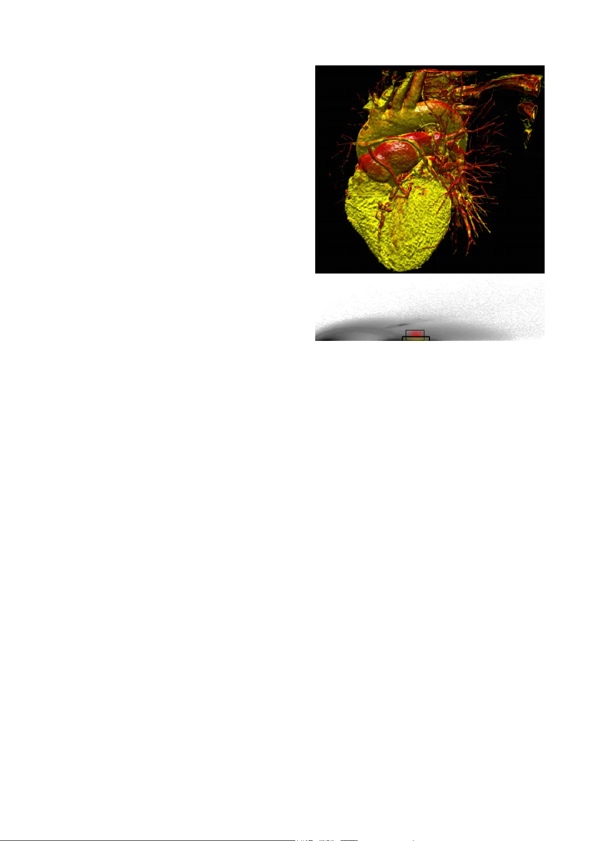
Ne ur al Ne tw or ks i n 3 D m e di c a l s c a n v i su a l i z at i o n Dženan Zukić, Dipl. Ing., dzenanz@gmail.com Hotonj II br. 52, 71322 Vogošća, Bosnia and Her zegovina University of Sarajevo / Facult y of Electrical Engineering / Computer Science Department Andreas Elsner, Dipl. Inf., trinet@uni-paderborn.de Warburger Strasse 100, D-33098 Paderborn, German y; Office: E3.118 University of Paderborn / Computer Sci. / C omputer Graphics / Visualization and Image Processin g Zikrija Avdagić, Prof. Dr., zikrija.avdagic@etf.unsa.ba ETF, Zmaja od Bosne bb - Kampus, 71000 Saraje vo, Bosnia and Herzegovina University of Sarajevo / Electrical Engineering / Computer Science / Artificial Intelligence Gitta Domik, Prof. Dr., domik@uni-paderborn.de Warburger Strasse 100, D-33098 Paderborn, German y University of Paderborn / Department of Computer S cience / Research Group Computer Graphics Abstract For medical volum e visualization , one of th e most imp ortant tasks is to reveal clinicall y relevant details from the 3D scan (CT, MRI …), e.g. the coronary arteries, without obscuring them with less significant parts. These volume datasets contain differe nt materials which are difficult to extract and visualize with 1D transfer functions based sol ely on the attenuation coe fficient. M ulti-dimensional transfer functions allow a much more precise classification of dat a which m akes it e asier to s eparate different s urfaces from e ach other. Unfortunatel y, setting up multi-dimensional transfer func tions c an become a fairly complex task, generall y accomplished by trial and error. This paper explains neural networks, and then presents an efficient wa y to spe ed up visualization process b y semi -automatic transfer fun ction generation. We describe how t o use neural networks to detect distinctive features shown in the 2D histogram of the volum e data and how t o use t his information for data classification. Keywords Neural networks, CT scans, medical visualiz ation software, 2D transfer functions Introduction For visualization and anal ysis of CT data (or any other 3D medical scan, like MRI or PET), the ke y advanta ge of dire ct volume rendering is the potential to show the three dimensional structure of a f eature of interest, rather than just a small part of the data b y cutting plane. This helps the viewer's perception to find the relative 3D positions of the object components and makes it easier t o detect and understand complex phenomena like coronary stenosis for diagnostic and operation planning [9]. One of the most basi c requirements of good volume visualization is a sophisticated way t o extract data that is actuall y o f interest, while suppressing insignificant parts. A lot of progress has been made in t he development of transfer functio ns as a feature classifier for volume data. The role of transfer function s is basically to assign specific visual attribut es like color and opacit y to the features of interest. The simpl est appro ach would be to use th e voxel data as the onl y variable to which these visual attributes are assi gned. But thi s method fails i n m ost cases to omit in terference of other anatomical structur es, be cause d atasets created from CT scans contain a combination of different materials and tiss ue types with overlapping boundaries. These stru ctures ma y contain the s ame range of data values making i t impossible for 1D transfer functions to differentiate between them. Instead of classifying the volume data on ly by the scalar value of its voxels, multi- dimensional transfer functions solve this problem b y addin g additional dim ensions to t he transfer function domain. By usin g a classification based on a combinati on of properties, different f eatures can then be visualized separately from each other. Therefore two dim ensional transfer functions can be used for the classification process which, in addition to the attenuation coefficient, also takes the cor responding gradient magnitude into account. At this time there ex ist different approaches to the design of transfer fun ctions, which become more widel y propagated [1], [2]. One of the most effective ways is the u se of manually editable, multi- dimensional transfer functions [3]. For this purpose, the software “VolumeSt udio” was developed capable of visualiz ing bot h modalities. Unfortunately, specif ying two-dimensional transfer functions can be come a fa irly compl ex and time-consumin g task. First, the user must handle additi onal parameters for the second dimension, thus making the editing process more difficult. Second, the user mu st set the transfer function i n the rather abstract transfer function domain while observing the result in the rendered im age (spatial domain). The situation is made worse by the fact that small changes t o these parameters t end sometimes t o cause lar ge and unpredictable changes to the visualization. Thus, to avoid editing based completely on trial and error, i t is ne cessary to identify features of interest in the transf er function dom ain first, requiring a good understanding of the data values and their relevance for a certain feature. Additio nally, the manual assi gnment of optical properties might be non-standardiz ed but rather influenced by the personal taste of the us er. This can caus e misint erpretation of the data if the vi sualization i s l ater on reviewed b y others. Also, this often lea ds to results which are hardly reproducible and hence not sui table for clinical practice. Finally, radiologist have a limited time allowed for diagnostics per patient, whi ch makes two-dimensional transfer functions impractical to use wit hout proper guidance throu gh the process or a semi - automatic transfer function generation. This paper presents a new appr oach for two- dimensional transfer function generation based on neural networks. Although t his technique is flexible enough f or classification of different types of CT dataset, in this paper we focus on heart scan visualiz ation to detect coronary diseases. As histograms of same scan t ype (e. g. heart s cans) have similar structures (same basic shape), neur al networks can be trained to position fil ters on feature s of int erest accordin g to the diagnostic target. Some of the related work can be found in [4] and [5]. Volume rendering For the volume rendering of scalar volume data like CT scans, different approaches ex ist. Texture based t echniques have p roved superior, combining high qualit y i mages and interactive frame rates. These appr oaches t ake advantage of th e hardware support of bilinear and trilinear interpolation provided by mode rn graphic cards, making hi gh quali ty visualization available on low cost commercial person al computers. For these approaches the dataset i s stored in the graphics hard ware texture memory first. If t he size of the d ataset exceeds the available memor y, bricking can be used to render the d ata in mu ltiple steps. The dataset is then sampled, using hardware interpolation. 2D texture-based app roaches use three copies of t he volum e data which resides i n t exture memory. E ach copy cont ains a fixed number of slices along a major axis of the dataset which will be addressed dependi ng on the current view direction. After bilinear interpolation, the values of the slices will then be classified through a lookup table, rendered as a planar polygon and blended i nto the image pl ane. This method often suffers from artifacts caused b y the fixed number o f slices and their static alignment along the major ax es. Alternativel y, hardware ext ensions can be used for intermediate slices alo ng the slice axis to achieve better visual qualit y. Modern graphics cards support 3D texture mapping whi ch allows storing the whole dataset in one 3D te xture. It is then possible t o sample view-aligned slices using tril inear interpolation. This approach avoids t he artifacts which occur when 2D te xture-based techniques switch between th e orthogonal slic e stacks an d allows an arbitrary s ample rate, which results in an overall b etter image quality. Also, no additional copies of the dataset are necessar y, lowering the requirements of tex ture memory. Transfer functions The value o f volume rendering in medicine, science and other fields of application not only depends on the visual qu ality achieved with th e rendering process its elf, the most important task is to find a good classification technique that captures the features of interest while suppressing insignificant par ts. As mentioned above, classification can be achieved b y transfer functions, which assign render able optical prope rties l ike color and op acit y to t he values of the dataset. 2D transfer fun ctions cl assify the volum e not just on the data values b ut on a combination of different prop erties and t herefore the boundaries of di fferent structures in the dataset can be better isolated as with 1D transfer functions. This is because the structures and tissue t ypes which are to be separated m ight lie within the same interval, making 1D transfer functions unable to render them in i solation. Kniss et al. presented a m ethod for manual multi-dimensional transfer function generatio n based on the data values and its derivatives [3] . The gradient is useful as an addit ional criterion for classification since it di scriminates between homogenous regions in side a structure and regions of ch ange at t he boundaries. Also, the gradient can b e used to appl y illumination t o the volume vi sualization which i mproves depth perception. The manual editing is perform ed in a visual editor, which i llustrates the distribution of tup les o f attenuation c oefficient and gradient magnitude of the dataset i n a joint histogram. The attenuation coefficient i s shown on the x- axis, the gradient magnitude on the y-axis. An example is given in Figure 1. Figure 1 2 D joint histo gram o f attenua tion co efficient versus g radient mag nitude . R egions a) – e) identify different mate rials. Homogeneous regions appear as cir cular spots at the bot tom of the histogram, as their gradient magnitude is ver y l ow. Five basic regions can be i dentified: a) air, b) soft t issue like fat and skin, c) muscles, d) blood (w ith contrast a gent) and e) bones. Arches between these s pots represent the boundaries of these regions. To create a new transf er function, the use r places filters inside the hi stogram, shown as rectangular areas. Each fi lter assigns color and opacity v alues to the vox els of the dataset which a re re presented by the tuples of attenuation coefficient and gradient in the histogram insi de the defined area. The filter size and pos ition can be c hanged, also its color and opa city d istribution. Also, the shape of the filter kernel can be altered between G auss and sine shape. If mu ltiple filters are set, their color and opacity values are blended t ogether. The above editing can be done i nteractively, and the user can decide by observing t he visualiz ation in the spatial domain if the current setup is appropriate or not . Through this feedback it is also possible to identify which regions o f the transfer function correspondents to the features of the dataset. Figure 2 shows a volume renderin g of a CT scan of the heart and the transf er fun ctions used. It consi sts of two gauss filters: The first one colored in y ellow i s located between the regions c) and d) (compare Figure 1) t o visualize t he m yocardial muscle and the coronaries (by contrast agent). Th e second one resides at t he top of the first filter, enhancing the contrast b etween m yocard and coronaries by coloring the properties t hat represent t he boundaries of the contrast agent in red. For an experienced user, the distinctive features of t he di stribution shown in the histogram provide useful in formation about the fe atures metrics, thereb y guiding the transfer function generation. But even with these hints, thi s is a time-consuming iter ative process. The user has to explore t he dataset b y de fining filters and move them t o possible interesting loc ations on the histogram. Onc e a feature of i nterest i s identified, the parameters for th e filter size, location, filter kernel shape, opacit y and color have to be optimized to match wit h the user’s needs until all features of interest are m ade visible. Figure 2 Volu me rende ring of a tho racic CT scan classified with a 2D transfer functio n Neural networks A neural network is a structure i nvolving weighted inter connections among neurons (which are most often nonl inear sca lar transformations). A neuron is structured to process multiple inputs, usually includin g the unity bias, in a nonlinear wa y, producing a single out put. Specifically, all inputs to a neuron are first augmented b y multiplicative weights. These wei ghted inputs are summed and then tr ansformed via a nonli near activati on function . The weights are som etimes referred to as synaptic strengths . The general pu rpose of the Neural Networks can be described to be function approximation. When inpu t data originates from a function with real-valued output s over a continuous range, the n eural networ k is said to perform a function approxi mation. An example of an approximation problem is when we control some process parameter by calculatin g a value of certain (complex ) function. I nstead, we could make a neural net work that approximates that function, and a neu ral network calculates output very quickly. Figure 3 Neural cell - neuron The f eed-forward, b ack-propagation network architecture was developed in the earl y seventies. Th e i nitial idea is credited t o va rious individuals, most prominently D.B Parker, P .J Werbos, G.E Hinton, R .J Williams, and D.E Rumelhart. One of t he most comm onl y used networks is the multila ye r fe ed forward network, also called multi-la yer preceptron. It has widespread interesting applications. We have isolated this specific netwo rk t ype as the neural n etwork w e have used ourselves. Feed-forward networks are advantageous as they are the f astest m odels t o ex ecute, and are universal function appr oximators. One major disadvantage of this n etwork t ype is that no fast and reliabl e trainin g algorithm has yet been designed and t herefore can be extremel y slow to train. Thus, multilayer feed-forward networks should be chosen if rapid execution rates are requi red, but slow learning rates are not a problem. Feed-forward networks usually consist of three or four la yers in which the neurons are logically arranged. The first and last layer s are the input and output layers respectivel y and there are usuall y one or more hidden la yers in between them. Res earch indicates that a minimum of three layers is required to solve complex problems [ 6]. Th e term feed-forward means that the informati on is onl y allowed to "travel" in one direction (there are no loops in networks). Furth ermore, this means th at th e output of one lay er becomes the input of the next layer, and so on. In order for t his to happen, each la ye r is full y connected to nex t layer ( each neuron is connected by a weight to a neuron in the next layer. Depending on implementation, input la y er can just dis tribute data to s econd layer, or it can subject inputs to thresho ld (if implemented in network) and activation function. The output of each neuron (except of those in input layer) is computed like:                , i –previous layer, j – current la yer, y – output, f – activation function,  – threshold (if implemented in network). For input layer:           . In order to train the neural network, sets of known i nput-output d ata points must be assembled. In other words, the neural network is trained by example ; m uch like a small child learns to speak. The mo st common and widely used algorithm for multi-layer feed-forward neural netwo rks is the back-propagation algorithm. The al gorithm starts by comparing actual output of t he network for the presented input with the desired output. The difference is called output er ror, and we try t o mi nimize it [8]. For each output in the output layer e rror delta is calculated:               , where    is first derivative of the activation function in that output neuron for the point of its output. Figure 4 Logistic ac tivation func tion The need to calculate derivatives in the p rocess of backpropagation explains t he usual choice of the activation function: logistic (    ) or hyperbolic tangent (       ). The main reason is that derivatives of the se functions can be calculated us ing the value of the function. For logistic function, which wa s used in our neural network, equality hol ds:          . Activation functions have to be diff erentiable in order to apply backpropagation. After w e have error delt as in the output l ayer, we can upd ate weights le ading into it, using th e following rule: !      "       , where " is learning rate (sm all value, usually betw een 0.05 and 0.3 ),   is er ror delta o f the neuron weight is leading into,   i s o utput of the neuron weight is comi ng from (output produced in t he fe ed-forward pro cess). Thi s rule is subsequentl y used for all wei ghts. Weights can be update d individuall y (called on-line learning) o r in groups (called b atch learning). In batch learning, we cal culate weight deltas for all samples, and then combine them in one single update. Batch update is usually better, as it lowers oscillations of the weights. For all layer s except output, error deltas are calculated us ing rule:               , i – current la yer, j – nex t layer. W e proceed backwards to the first lay er calculating error deltas and updating w eights. When the weights between 1 st and 2 nd la yer are updat ed, backpropagation is finished. The training process is repeated man y times (epochs) until satisfactory result s are obtained. Training can stop when the error obtained is less than a certain limit , or we have reached some pre-set maximum number of tr aining epochs [7]. It is important to say th at "over-training" of a network should be avoided, as it lowers predictive abilities of the network, as it i s said that network learns “details of the t raining s et”. Examples that the network is unfamiliar wit h, form what is known as the validation set, which tests the network's cap abilities before it is implemented for use. Solution of the problem Knowing the properties of 2D histograms and 2D transfer functions on one hand, and having some experience in ne ural networks on t he other, we conceived a soluti on to the problem. As stated in transf er fun ctions section, the 2D histogram showin g the distribution of tuples of attenuation coefficient and gradient m agnitude of a heart dataset contains dis tinctive features which can be used t o guide the transfer function setup. These features consist of circular spots at the bottom of the hist ogram representing homo geneous m aterials and arches which d efine material bound aries. Hence, the poison and siz e of a filter setup for a 2D transfer function depends on those patterns. Given as an input, the histogram can be used to train a neural network f or pattern recognition. Therefore the user creates filter setups for a training set manually acc ording to the diagnostic target. The network is then trained to associate outputs (filters) with input patterns in the hi stogram. This time consuming st ep has only to be p erformed once a nd can b e done outside clinical practice. Once the network is properly trained, it can be used to c reate a n appropriate filter setup automaticall y. The 2D histo gram is basicall y a gra yscale image with dimensions 256*256. An input of this size would require a significant amount of memory for storage (16 MB just for weights in case of 64 neurons in 2 nd layer). Also, training of such a network would b e slow, and its generalization abilities would be presumabl y low. Therefore, as a p reprocessing step, the input to the neural network must be reduc ed to data that is relevant for the patte rn recognition. First, w e removed those parts o f the histogram t hat contain no data at all. Since the size of the u sed part in the his togram v aries from dat aset to dataset, we estimated a maxi mum size based o n the training set and us e t his as a fixed value for all datasets of the same type. For the he art CT scans used to evaluate our approach i t is sufficient t o re move the upper half of the histogram and onl y take the lower one into account. Second, we downscaled the remaining histogram b y a f actor o f 4. This reduces the number of inputs to the neural network to just 2048. Furthermore, the downscaling of the image smoothes out parts of the histogram which lie outside the distinctive features required for pattern recognition. Since these parts consists of tuples of a t t e n u a t i o n coefficient and g radient mag nitude w h i c h h a v e only a few voxels of the dataset a s s i g n e d t o them, the y appe ar to the neural n e t w o r k a s noise. Also, these parts vary a l o t b e t w e e n different datasets. As this affects t h e l e a rate, wit h noise removed and i m a g e s i z e reduced, t he neur al n etwork wil l l e a r n m o r e easily and will have better g e n e r a l i z a t i o n abilities. Figure 5 Original and reduced h istogr a m As two gauss filters are usua l l y u s e d t o visualize heart and its arteries, we d e c i d e d t h a t output of our network would be p o s i t i o n s a n d sizes of those ga uss filters. H enc e , n u m b e r o f outputs i s 8 (xpos1, ypos1, xs i z e 1 , y s i z e 1 , xpos2, y pos2, xsize2, y size2). That leaves some v ariabilit y f o r l a y e r s between. We started with 1 hi dde n l a y e r w i t h 64 neurons i n it. We worke d w i t h t h i s architecture throughout software d e v e l o p m e n t until final training and testi ng, w h i c h i s w h e n we did some exp erimentation. W e r e d u c e d s i z e of t he hid den la yer first t o 32 an d t h e n t o 1 6 , and noticed no deg radation in resu l t s . W e k e p t 16 neurons in hidden la yer. W e d i d n o t experiment with more than 1 hid d e n l a y e r ( a s there was no need for it). Trying t o see how many sample s n e e d t o b e used for t raining in ord er for n eur a l n be useful, we did some ex periment a t i o n . F o r 1 2 samples, we manually determin e d p o s i t i o n s . Then 2 samples we marked as con t r o l s a m p l e s (validation samples), and other 1 0 w e r e u s e d for training. W e created 5 neural n e t w o r k s , f i r s t c o n s i s t s o f t u p l e s o f attenuation c o e f f i c i e n t a n d g r a d i e n t m a g n i t u d e which h ave o n l y a f e w v o x e l s o f t h e d a t a s e t assi gned to t h e m , t h e y a p p e a r t o t h e n e u r a l network as n o i s e . A l s o , t h e s e p a r t s v a r y a lot between d i f f e r e n t d a t a s e t s . A s t h i s a f f e c t s the lea rning r a t e , w i t h n o i s e r e m o v e d a n d ima ge siz e r e d u c e d , t h e n e u r a l n e t w o r k w i l l learn mor e e a s i l y a n d w i l l h a v e b e t t e r generalization O r i g i n a l a n d r e d u c e d h i s t o g r am A s t w o g a u s s f i l t e r s a r e u s u all y used to v i s u a l i z e h e a r t a n d i t s a r t e r i e s , w e decided that o u t p u t o f o u r n e t w o r k w o u l d b e positions and s i z e s o f t h o s e g a u s s f i l t e r s . H e n c e, number of o u t p u t s i s 8 ( x p o s 1 , y p o s 1 , x s ize1, y size1, T h a t l e a v e s s o m e v a r i a b i l i t y f or la yers in b e t w e e n . W e s t a r t e d w i t h 1 h i d d en layer with 6 4 n e u r o n s i n i t . W e w o r k e d with this a r c h i t e c t u r e t h r o u g h o u t s o f t w a r e development u n t i l f i n a l t r a i n i n g a n d t e s t i n g , w hich is when w e d i d s o m e e x p e r i m e n t a t i o n . W e reduced size a n d t hen to 16, a n d n o t i c e d n o d e g r a d a t i o n i n r e s ults. We kept 1 6 n e u r o n s i n h i d d e n l a y e r . We did not e x p e r i m e n t w i t h m o r e t h a n 1 h i d den layer (as T r y i n g t o s e e h o w m a n y s a m p l e s need to be u s e d f o r t r a i n i n g i n o r d e r f o r n e u r al n etwork to b e u s e f u l , w e d i d s o m e e x p e r i m e n tation. For 12 s a m p l e s , w e m a n u a l l y d e t e r m i n ed pos itions. T h e n 2 s a m p l e s w e m a r k e d a s c o ntrol samples ( v a l i d a t i o n s a m p l e s ) , a n d o t h e r 10 were used f o r t r a i n i n g . W e c r e a t e d 5 n e u r a l networks, first one trained with 2 samp l e s , s e c o n d o n e w i t h 4 samples and fifth one w i t h 1 0 s a m p l e s , a n d o n all of these networks w e u s e d 2 c o n t r o l s a m p l e s to check for error. On Fi g u r e series, one showin g e r r o r o f n e t w o r k s o n training data, and the o t h e r e r r o r s o n t e s t d a t a . For all networks exce p t f i r s t o n e ( t h e o n e trained with only 2 samp l e s ) , m e a n s q u a r e e r r o r is lower on test set, than o n t r a i n i n g s e t . T h i s i s unusual, but ca n be ex p l a i n e d w i t h f a c t t h a t positions that we ma n u a l l y p r o v i d e d f o r networks, were not all th a t s i m i l a r . It is qui te clear that e v e n s m a l l n u m b e r o f training s amples produc e s g o o d r e s u l t s . I n o u r measurements, networks t r a i n e d o n 6 , 8 , a n d 1 0 samples p ro vide nearl y t h e s a m e r e s u l t s a s network trained with ju s t 4 s a m p l e s . T h i s c a n be explained by the f ac t t h a t h i s t o g r a m s h a v e so typical shape, s o ju s t 4 t r a i n i n g s a m p l e s suffice for good re cognit i o n , a n d a l l k n o w l e d g e gained b y additional tra i n i n g i s a n n i h i “overfitting”, so trainin g t h e n e t w o r k b e y o n d basic needs achieves ver y l i t t l e e f f e c t . Also interesting is that t r a i n i n g M S E ( m e a n square erro r) jumps on n e t w o r k t r a i n e d w i t h 4 samples, and then g ra d u a l l y d e c r e a s e s w i t h increased numb er of trai n i n be ex plained wit h assum p t i o n t h a t e i t h e r o n 3 or 4 th sample training d a t a w a s “ r a d i c a l l y ” different from the othe rs , s o n e t w o r k c o u l d n o t easily minimiz e that e r r o r s t h a t i t s o d d i t y produces. As the numbe r o f s a m p l e s i n c r e a s e , relativ e influence of that s a m p l e i s r e d u c e d a n d MSE is lowered. Figure 6 Mean squ are erro r s o n n e t w o r k s t r a i n e d w i t h varying n umber o f train samp l e s 0.0000 0.0001 0.0002 0.0003 0.0004 0.0005 0.0006 0.0007 MSE on t r a i n i n g s e t MSE on v a l i d a t i o n s e t 2 s a m ples, second one with 4 s a m p l e s a n d f i f t h o n e with 10 samples, and on a l l o f t h e s e n e t w o r k s w e used 2 control s amples F igure 6, there are 2 data s e r i e s , o n e s h o w i n g error o f networks on t r a i n i n g d a t a , a n d t h e o ther errors on t est data. F o r a l l n e t w o r k s e x c e pt first one (the one t r a i n e d w i t h o n l y 2 s a m ples), mean square error i s l o w e r o n t e s t s e t , t h a n on training s et. This is n b e e xplained with fact th at p o s i t i o n s t h a t w e m anuall y provided for n o t a l l t hat similar. I t i s q u i t e c l e a r t h a t e ven small number of t r a i n i n g s a m p l e s p r o d u ces good results. In our m e a s u r e m e n t s , n e t w o r k s trained on 6 , 8, and 10 v i d e n e a r l y the same results as n e t w o r k t r a i n e d w i t h j u st 4 sampl es. This can b e e x p l a i n e d b y t h e f a ct that histograms have s o t y p i c a l s h a p e , s o j ust 4 training samples s u f f i c e f o r g o o d r e c o g n i tion, and all knowledge g a i n e d b y a d d i t i o n a l t r aining is annihi lated b y “ o v e r f i t t i n g ” , s o t r a i n i n g the ne twork beyond b a s i c n e e d s a c h i e v e s v e ry little effect. A l s o i n t e r e s t i n g i s t h a t training MSE (me an s q u a r e e r r o r ) j u m p s o n network tr ained wit h 4 s a m p l e s , a n d t h e n g r a duall y d ecreases with i n c r e a s e d n u m b e r o f t r a inin g samples. This can b e e x p l a i n e d w i t h a s s u mption that either on 3 rd s a m p l e t r a i n i n g data w as “radicall y” d i f f e r e n t f r o m t h e o t h e r s, so network could not e a s i l y m i n i m i z e t h a t errors that its oddity p r o d u c e s . A s t h e n u m b er of samples increase, e i n f l u e n c e o f t h a t sample is reduced and M e a n s q u a r e e r r ors o n networks tra ined with v a r y i n g n u m b e r o f t r a i n s a m ples M S E o n training set M S E o n validation set The neural network software built into VolumeStudio enables t o additi onally train existing neural netwo rk, and stand-alone training tool has also be created (wit h more features for training th an built-in function). This enables neural network to be retrained, or created from scratch on new datas et. Creating new neural network also enables creating specialized networks for other sp ecific bod y scans, like head or the whole bod y, for example (we did not h ave enou gh samples of those types to experiment with it ourselves). Conclusion and outlook The ti me spent on p ositioning the filt ers has been cut down from 1-3 minutes to approximately 10-30 seconds needed for fine tuning of the parameters after automatic filter generation, giving doctors more time to anal yze the data. Also, neural networks kick-start usefulness of VolumeStudio for new users. A num ber of things could have been done differently. First, histogram image downs caling could be b y factor of 2, not 4. We did not change that, because the results are satisfactor y as it i s done now. We could have experimented with different number of layers, to se e what results it would give. Also, as it i s now im plemented in software, the user has t o manually select an appropriate neural network to c reate the filters by the type of dataset (e.g. h eart, head or whole b ody scan) that has been loaded. One approach to autom ate this t oo, is to us e an additional network to classi fy input samples into type categories. This network has to have as man y output s as there are different n etworks for different data t ypes. When the user loads new scan, this data classi fication network is used to determine type of scan and after that, based on the output of t he classification network the appropriate network for filter positioning is chosen. T his approac h, however, has the small drawback t hat when ever you add a network for ne w sc an t ype, you have to change architecture of the classifier b y adding an addit ional output and subsequently re-train it. References [1] Engel, K., Hadwi ger, M., Kniss, J ., Rezk- Salama, C.: Real-Time Volum e Graphics. Eurographics Tutorial (2006) [2] Engel, K., Hadwi ger, M., Kniss, J ., Rezk- Salama, C., Weiskopf, D.: Real-Time Volume Graphics. AK Peters, Ltd, Wellesley, Massachusetts (2006) [3] J . Kniss, G. Kindlmann, C. Hansen. Multi- Dimensional Transfer Functions for Interactive Volume Rendering. IEEE Transactions on Visualization and Computer Graphics, 8(3): 270-285, J ul y , 2002 [4] J . Marks, B. Abdalman, P. Beardsle y, W. Freeman, S. Gibson, J. Hodgins, T. Kang, B. Mirtich, H. Pfister, W. Ruml, K. R yall, J. Seims, S. Shieber. Design Galleries: A General Approach to Setting Parameters for Computer Graphics and Animation. In Proceedings SIGGRAPH, 1997 [5] G. Kindlm ann, J. W. Durkin. Semi- Automatic Generation of Transfer Functions for Direct Volume Rendering. ACM Symp. On Volume Visualiz ation, 1998 [6] Zikrija Avda gić, Artificial Intelligence & Fuzzy-Neuro-Genetic , Grafoart Sarajevo, 2003. [7] Bernard Will ers and Sep Vrba, „Artificial Neural Networks: Emulating the Operation of the Human Brain“, August 2000, http://library.thinkquest.org/C007395/ . [8] D. Rum elhart, G. Hinton and R. Williams, „Learning representations b y back- propagating errors“, Nature, Vol. 323, pp. 533 – 536, October 1986. [9] Brochure „ Blick in das Herz “, Deutschen Gesellschaft für Nuklearmedizi n