State Estimation Over Wireless Channels Using Multiple Sensors: Asymptotic Behaviour and Optimal Power Allocation

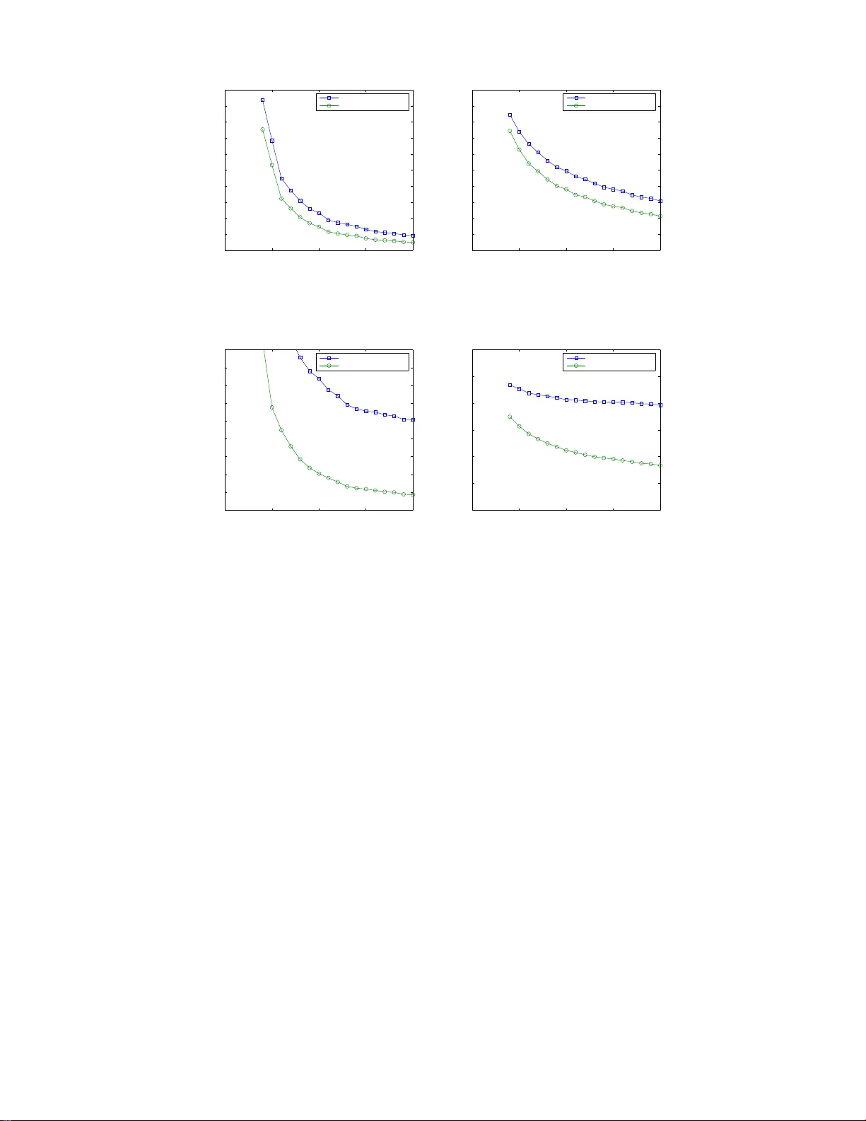
State Estimation Ov er W ireless Channels Using Multiple Sensors: Asymptotic Beha viour and Optimal Po wer All ocation Alex S. Leong, Subhrakanti Dey , and Jamie S. Evans Abstract This pa per con siders state estimation of linear systems usin g an alog amp lify and forwarding with multiple sensors, for both multiple access and o rthogo nal access schem es. Optim al state estimation can be achiev ed at the fusion center using a ti me varying Kalman ﬁlter . W e sh ow that in ma ny situations, the estimation er ror covariance decays at a rate of 1 / M wh en the number of sensors M is large. W e consider optimal allocation of transmission powers th at 1) minimizes the sum power usage subject to a n error cov ariance constraint and 2 ) minimizes th e error c ovariance subject to a sum power constra int. In the case of fading channels with channel state information the optimization problem s are solved using a gre edy approach, while for fading channels without channel state informa tion but with ch annel statistics av ailable a sub-o ptimal linear estimator is derived. Index T erms Distributed estimation, Kalma n ﬁltering , power allocation , scaling laws, sensor networks I . I N T RO D U C T I O N W ireless se nsor networks are collections of senso rs which can c ommunicate with each other or to a ce ntral node or b ase station throu gh wireless links . Potential us es include environment and infrastructure monitoring, healthca re and military applications , to name a few . Often these sens ors will ha ve limited energy and comp utational abilit y which imposes se vere constraints on system design, a nd s ignal processing algorithms which ca n e fﬁciently utilise these resources have attracted great interest. In recent years there has been a considerable li terature on estimation and detection scheme s de signed speciﬁca lly for use in wireless senso r n etworks. W ork on detection in wireless sens or networks include [1] which studies the asymptotic o ptimality o f using identical sensors in the presence of energy constraints, and [2]–[4] which deri ves fusion rules for distributed dete ction in the presenc e of fading. Parameter e stimation or estimation of constant signals is stud ied in e.g. [5]–[8] where issues o f qu antization a nd op timization of power us age are address ed. T ype based methods for detection and estimation of discrete sou rces are propose d and analyzed in [9]–[11]. Estimation of ﬁelds is considered ha s b een c onsidered in e.g. [12]–[14]. A promising sche me for distributed estimation in sensor networks is a nalog amplify and forward [15 ] (in distrib uted detection an alog forwarding h as also be en considered in e.g. [16], [17]), where meas urements from the sensors are transmitted directly (possibly scaled) to the fusion c enter without any coding, w hich is motiv ated b y optimality results on uncoded transmis sions in point-to-point links [18], [19]. (Other related information theoretic results include [20], [21].) Analog forwarding scheme s are attractive due to the ir simplicity as well as the pos sibility of real-time p rocessing since there is no coding de lay . In [15] the asymptotic (lar ge nu mber of s ensors) optimality of analog forwarding for estimating an i.i.d. scalar Gaussian process was shown, and exa ct o ptimality was later proved for a “symmetric” se nsor ne twork [22]. Analog forwarding with op timal power allocation is s tudied in [23] and [24] for multi-access and o rthogonal sch emes resp ectiv ely . Lower bounds an d asymptotic optimality res ults for estimating indep endent vector processe s, is addressed in [25]. Estimation with correlated data between sens ors is studied in [26 ], [27]. Other aspects of the analog forwading techn ique that have been studied includ e the use of The auth ors are wit h the ARC Special Research Center for Ultra-Broadband Information Networks (C UBIN, an afﬁliated program of National ICT Australia), Department of El ectrical and El ectronic Engineering, Univ ersity of Melbourne, Parkville, V ic. 3010, Australia. T el: 613-8344-3819 . Fax: 613-8344-667 8. E-mail { asleong , sdey, jse } @unimelb.edu.au This work was supported by the Australian Research Council 2 dif ferent network topolog ies [28], other multiple access schemes such as slotted ALOHA [29], and con sideration of the impac t of channel e stimation errors [30] on e stimation pe rformance. Most of the previous work on analog forwarding have dealt with estimation of proc esses which are e ither constant or i.i.d over time. In this paper we will ad dress the estimation of dyna mical sys tems using analog forwarding of measureme nts. In particular , we will consider the problem of state estimation of disc rete-time linear s ystems using multiple sensors. As is well known, op timal state estimation of a linear system can be ach iev ed using a Kalman ﬁlter . Other work on Kalman ﬁltering in senso r networks include studies of optimal sensor d ata qua ntization [31], Kalman ﬁltering using one bit quantized observations [32] where performance is sh own to lie within a cons tant factor of the s tandard Kalman ﬁlter , a nd estimation of rand om ﬁelds with redu ced orde r Kalman ﬁlters [14]. Anothe r related area with a rich history is that o f distributed Kalman ﬁltering, wh ere the main objecti ves include do ing local process ing at the individual se nsor le vel to reduce the computations required at the fusion center [33], [34 ], or to form es timates at ea ch of the individual sensors in a completely de centralized fashion without any fusion center [35]. Howev er in o ur work we assume that co mputational resources av ailable at the sensors are limited so that they will only take mea surements and then trans mit them to the fusion cen ter for further proce ssing, using uncode d analog forw arding. Summary of Contributions : In this paper we will mainly focu s on estimation of sca lar 1 linear dyna mical systems u sing mu ltiple sen sors, as the vector case introduces additional difﬁculties suc h that on ly p artial results can b e obtained. W e will be interested in deriving the as ymptotic be haviour of the error covari ance with respect to the numbe r of sensors for the se s chemes , as we ll a s optimal transmission po wer a llocation to the sensors under a cons traint on the e rror cov ariance at the fusion center , or a sum po wer cons traint at the se nsor transmitters. W e consider bo th s tatic an d f ading channels, and in the co ntext of fading ch annels, we con sider various lev els of av ailability of channel s tate information (CSI) at the transmitters and the fusion center . More spec iﬁcally , we make the follo wing key c ontributi ons: • W e show that (for static channels with full CSI) for the mu lti-access s cheme, the asymptotic e stimation error covari ance ca n be dri ven to the proce ss no ise covariance (which is the minimum attainable error) a s the numb er of sensors M g oes to inﬁnity , ev en when the transmitted signals from each sen sor is s caled by 1 √ M (which implies that total trans mission power ac ross all sensors remains boun ded while e ach senso r’ s transmission power goe s to zero). This is a p articularly attracti ve res ult since sensor networks ope rate in a ener gy limit ed en vironment. For the orthogon al acc ess sc heme, this result holds when the transmitted signals are unscaled, but does not ho ld when the transmitted sign als are scaled by 1 √ M . • T he con ver gence rate of thes e asymptotic results (when they hold) is shown to be 1 M , although it is seen via simulation results that the asymptotic app roximations are quite a ccurate even for M = 20 to 30 sens ors. • In the cas e of a small to mo derate number o f sensors, we derive a comprehens iv e set of optimal sens or transmit po wer a llocation sch emes for multi-access a nd orthog onal med ium a ccess schemes over both static and f ading channels. For static c hanne ls, we minimize total transmiss ion power at the sensors sub ject to a constraint on the steady state Kalman estimation error covariance, an d also solve a correspon ding co n verse problem: minimizing stead y state error covariance s ubject to a su m power c onstraint a t the s ensor transmitters. For fading channels (with full CS I), we solve similar optimization problems, except tha t the error cov ariance (either in the objectiv e function or the con straint) is cons idered at a p er time instant ba sis, since there is no we ll deﬁned stead y s tate error c ov ariance in this case. For the fading chan nel case with n o CSI (either amplitude or phase), the results are de ri ved for the best linear es timator which relies on chan nel s tatistics informati on and can be a pplied to non-ze ro mea n fading channels. It is shown that these optimization problems can be pose d as con vex optimization problems. Moreover , the optimization problems will turn out to be very similar to problems previously s tudied in the literature (albeit in the con text of distributed estimation of a static ran dom source), namely [23], [24], and can actually be solved in closed form. • N umerical resu lts demon strate that for static cha nnels, op timal power a llocation res ults in mo re bene ﬁt for the orthogonal medium acces s sche me compared to the multi-access sc heme, w hereas for fading c hannels , it is seen tha t having full CSI is clearly be neﬁcial for both s chemes , althou gh the performance improvement v ia the optimal power allocation scheme is more substa ntial for the orthogonal sche me than the multi-access scheme . The rest of the paper is or ganized a s follo ws. Sec tion II speciﬁes our sca lar models and preliminaries, and 1 By scalar linear system we mean that both the states and indiv idual sensor measurements are scalar . 3 giv es a number of examples between multi-access and orthogon al access schemes , which s how tha t in general one sc heme doe s not always pe rform better tha n the other . W e inv estigate the as ymptotic behaviour for a lar ge number of s ensors M in Section II I. Power allocation is considered in Sec tion IV, where we formulate and solve optimization problems for 1) an error covari ance constraint and 2) a sum power constraint. W e ﬁrst do this for static channels, b efore focu sing o n fading cha nnels. In the case where we hav e chan nel state information (CSI) we use a gree dy ap proach by performing the optimization a t each time step. When we don ’ t have CSI, we will deri ve a sub-optimal linea r e stimator similar to [36]–[38], which can be used for non-zero mean fading. Numerical s tudies are presented in Section V. Extensions of our model to vector and MIMO sy stems is considered in Section VI, where we formulate the mod els a nd optimization problems, and ou tline some of the difﬁculties in v olved. I I . M O D E L S A N D P R E L I M I NA R I E S Throughou t this pa per , i represents the se nsor ind ex and k represen ts the time index. Le t the sca lar linear s ystem be x k +1 = ax k + w k with the M sensors ea ch obs erving y i,k = c i x k + v i,k , i = 1 , . . . , M with w k and v i,k being zero-mean Ga ussians having variances σ 2 w and σ 2 i respectively , with the v i,k ’ s being independ ent betwe en sensors. Note that the sens ors can ha ve different observation matrices c i and measureme nt noise v ariances σ 2 i , and we allo w a and c i to ta ke on both pos iti ve and negative values. It is ass umed that the parameters a, c i , σ 2 w and σ 2 i are k nown. 2 Furthermore, we assume that the system is stable, i.e. | a | < 1 . A. Multi-acces s s cheme In the (non-orthogo nal) multi-acce ss sc heme the fusion center rece i ves the sum ˜ z k = M X i =1 ˜ α i,k ˜ h i,k y i,k + ˜ n k (1) where ˜ n k is zero-mean complex Gau ssian with variance 2 σ 2 n , ˜ h i,k are the complex-valued channe l gains, a nd ˜ α i,k are the complex-valued multiplicativ e a mpliﬁcation f actors in an amplify a nd forward scheme. W e assume that all transmitters have acce ss to the ir complex c hanne l s tate information (CSI), 3 and the ampliﬁcation factors hav e the form ˜ α i,k = α i,k ˜ h ∗ i,k | ˜ h i,k | where α i,k is real-v alued, i.e. we as sume distrib uted transmitter bea mforming. Deﬁning h i,k ≡ | ˜ h i,k | , z k ≡ ℜ [ ˜ z k ] , n k ≡ ℜ [ ˜ n k ] , we then ha ve z k = M X i =1 α i,k h i,k y i,k + n k (2) Note that the as sumption of CSI a t the transmitters is important in order for the signals to a dd u p co herently in (2). In principle, it can b e achieved by the distributed synchron ization sche mes des cribed in e.g. [39], [40], but may not be fea sible for large se nsor n etworks. Howev er , in studies such as [16], [39] it has been shown in s lightly different contexts that for mode rate a mounts of pha se error much o f the potential performance gains can still be achieved. Continuing furt her , we may write z k = M X i =1 α i,k h i,k c i x k + M X i =1 α i,k h i,k v i,k + n k = ¯ c k x k + ¯ v k 2 W e assume that these parameters are static or very sl o wly ti me-v arying, and hence can be accurately determined beforehand using appropriate parameter estimation/system identiﬁcation algorithms. 3 The case where the channel gains are unkno wn but channel statistics are av ailable is addressed i n Section IV -E. This can also be used to model the sit uation where perfect phase synchronization cannot be achiev ed [ 25]. 4 where ¯ c k ≡ P M i =1 α i,k h i,k c i and ¯ v k ≡ P M i =1 α i,k h i,k v i,k + n k . Hence, we have the follo wing linear sys tem x k +1 = ax k + w k , z k = ¯ c k x k + ¯ v k (3) with ¯ v k having variance ¯ r k ≡ P M i =1 α 2 i,k h 2 i,k σ 2 i + σ 2 n . Deﬁne the state e stimate an d e rror cov ariance a s ˆ x k +1 | k = E [ x k +1 |{ z 0 , . . . , z k } ] P k +1 | k = E  ( x k +1 − ˆ x k +1 | k ) 2 |{ z 0 , . . . , z k }  where again P k +1 | k is scalar . T hen it is well known that optimal e stimation of the state x k in the minimum mean squared error (MMSE) sens e ca n be achieved using a (in gene ral time-varying) Kalman ﬁlter [41]. Using the shorthand notation P k +1 = P k +1 | k , the error cov ariance satisﬁe s the recursion: P k +1 = a 2 P k − a 2 P 2 k ¯ c 2 k ¯ c 2 k P k + ¯ r k + σ 2 w = a 2 P k ¯ r k ¯ c 2 k P k + ¯ r k + σ 2 w (4) W e also remark that e ven if the noise s are non-Gaus sian, the Kalman ﬁlter is still the best linear estimator . B. Orthogon al ac cess sche me In the orthogonal access scheme e ach sensor transmits it s meas urement to the fusion cen ter via orthogon al channe ls (e.g. using FDMA or CDMA), so that the fusion center rece i ves ˜ z i,k = ˜ α i,k ˜ h i,k y i,k + ˜ n i,k , i = 1 , . . . , M with the ˜ n i,k ’ s being indepe ndent, zero me an complex Gaus sian with v ariance 2 σ 2 n , ∀ i . W e w ill again as sume CS I at the tr ansmitters and use ˜ α i,k = α i,k ˜ h ∗ i,k | ˜ h i,k | , with α i,k ∈ R . Let h i,k ≡ | ˜ h i,k | , z i,k ≡ ℜ [ ˜ z i,k ] , n i,k ≡ ℜ [ ˜ n i,k ] . The situation is then equiv alent to the linear system (using the s uperscript “ o ” to distinguish some quantities in the orthogonal scheme from the multi -acces s sch eme): x k +1 = ax k + w k , z o k = ¯ C o k x k + ¯ v o k where z o k ≡    z 1 ,k . . . z M ,k    , ¯ C o k ≡    α 1 ,k h 1 ,k c 1 . . . α M ,k h M ,k c M    , ¯ v o k ≡    α 1 ,k h 1 ,k v 1 ,k + n 1 ,k . . . α M ,k h M ,k v M ,k + n M ,k    with the covariance of ¯ v o k being ¯ R o k ≡      α 2 1 ,k h 2 1 ,k σ 2 1 + σ 2 n 0 . . . 0 0 α 2 2 ,k h 2 2 ,k σ 2 2 + σ 2 n . . . 0 . . . . . . . . . . . . 0 0 . . . α 2 M ,k h 2 M ,k σ 2 M + σ 2 n      The state estimate and error covariance a re now de ﬁned a s ˆ x o k +1 | k = E [ x k +1 |{ z o 0 , . . . , z o k } ] P o k +1 | k = E h ( x k +1 − ˆ x o k +1 | k ) 2 |{ z o 0 , . . . , z o k } i Optimal estimation of x k in the orthogo nal access sche me can also be achieved using a Ka lman ﬁlter , with the error c ov ariance now satisfying the recursion: P o k +1 = a 2 P o k − a 2 ( P o k ) 2 ¯ C o T k ( ¯ C o k P o k ¯ C o T k + ¯ R o k ) − 1 ¯ C o k + σ 2 w where ¯ C o k and ¯ R o k as deﬁned above are respectiv ely a vector and a matrix. T o simplify the expressions, note that ¯ C o T k ( ¯ C o k P o k ¯ C o T k + ¯ R o k ) − 1 ¯ C o k = ¯ C o T k ¯ R o − 1 k ¯ C o k 1 + P o k ¯ C o T k ¯ R o − 1 k ¯ C o k , 5 which can be shown u sing the matrix in version lemma. Henc e P o k +1 = a 2 P o k 1 + P o k ¯ C o T k ¯ R o − 1 k ¯ C o k + σ 2 w (5) where one can also eas ily c ompute ¯ C o T k ¯ R o − 1 k ¯ C o k = P M i =1 α 2 i,k h 2 i,k c 2 i / ( α 2 i,k h 2 i,k σ 2 i + σ 2 n ) . The advantage of the orthogonal scheme is tha t we d o no t ne ed c arrier -le vel s ynchroniza tion among all s ensors, but only requ ire synchron ization between each individual sen sor and the fusion cen ter [24]. C. T ransmit powers The power γ i,k used at time k b y the i th sensor in transmitting its meas urement to the fusion cen ter is d eﬁned as γ i,k = α 2 i,k E [ y 2 i,k ] . For stable s calar sys tems, it is well known tha t if { x k } is stationary we have E [ x 2 k ] = σ 2 w 1 − a 2 , ∀ k . In both the multi-access an d orthog onal schemes, the transmit powers are then: γ i,k = α 2 i,k  c 2 i σ 2 w 1 − a 2 + σ 2 i  D. Stea dy state err or covar iance In this and the next few s ections we will let ˜ h i,k = ˜ h i (and he nce h i,k = h i ) , ∀ k be time-in vari ant, deferring the discuss ion of time-v arying channels until Section IV -D. W e will also as sume in this case that α i,k = α i , ∀ k , i.e. the ampliﬁcation factors don’t vary with time, and we will drop the subscript k fr om q uantities such as ¯ c k and ¯ r k . From Kalman ﬁltering the ory , we know that the steady state (as k → ∞ ) e rror covariance P ∞ (provided it exists) in the multi-acces s sch eme sa tisﬁes (c.f.(4)) P ∞ = a 2 P ∞ ¯ r ¯ c 2 P ∞ + ¯ r + σ 2 w (6) where ¯ r and ¯ c are the time-in variant versions of ¯ r k and ¯ c k . 4 For stable systems , it is kn own that the steady state error c ov ariance always exists [41, p.77 ]. For ¯ c 6 = 0 , the solution to this ca n b e e asily sho wn to be P ∞ = ( a 2 − 1) ¯ r + ¯ c 2 σ 2 w + p (( a 2 − 1) ¯ r + ¯ c 2 σ 2 w ) 2 + 4¯ c 2 σ 2 w ¯ r 2¯ c 2 (7) In the “d egenerate” case w here ¯ c = 0 , we have P ∞ = σ 2 w / (1 − a 2 ) . It will also b e u sful to write (7) a s P ∞ = a 2 − 1 + σ 2 w S + p ( a 2 − 1 + σ 2 w S ) 2 + 4 σ 2 w S 2 S (8) with S ≡ ¯ c 2 / ¯ r regarded a s a signal-to-noise ratio (SNR). W e hav e the follo wing property . Lemma 1: P ∞ as deﬁned by (8) is a decreasing function of S . Pr oof: See the Append ix. Similarly , in the orthogonal acce ss sc heme, the steady s tate error covariance P o ∞ satisﬁes (c .f.(5)) P o ∞ = a 2 P o ∞ 1 + P o ∞ ¯ C o T ¯ R o − 1 ¯ C o + σ 2 w (9) where ¯ R o and ¯ C o are the time-in v ariant versions of ¯ R o k and ¯ C o k . W e can easily compute ¯ C o T ¯ R o − 1 ¯ C o = P M i =1 α 2 i h 2 i c 2 i / ( α 2 i h 2 i σ 2 i + σ 2 n ) w ith S o ≡ ¯ C o T ¯ R o − 1 ¯ C o regarded as a signa l-to-noise ratio. The solution to (9) can then be foun d a s P o ∞ = a 2 − 1 + σ 2 w S o + p ( a 2 − 1 + σ 2 w S o ) 2 + 4 σ 2 w S o 2 S o (10) Lemma 2: P o ∞ as deﬁned by (10) is a decreasing function of S o The proof is the s ame as that of Le mma 1 in the Appe ndix. 4 The assumption of time-inv ariance is important. For time-varying ¯ r k and ¯ c k , the error cov ariance usually will not con ver ge to a steady state value. 6 Comparing (8) and (10) we see that the functions for P ∞ and P o ∞ are of the sa me form, exc ept that in the multi-access s cheme we have S ≡ ¯ c 2 ¯ r =  P M i =1 α i h i c i  2 P M i =1 α 2 i h 2 i σ 2 i + σ 2 n and in the orthogonal s cheme w e h av e S o ≡ ¯ C o T ¯ R o − 1 ¯ C o = M X i =1 α 2 i h 2 i c 2 i α 2 i h 2 i σ 2 i + σ 2 n E. So me examples of multi-access vs orthogonal acces s A natural question to a sk is whether one s cheme always performs better than the other , e.g . w hether S ≥ S o giv en the same values for α i , h i , c i , σ 2 i , σ 2 n are used in both express ions. W e presen t below a numb er of examples to illustrate that in general this is not true. Assume for simplicity that the α i ’ s are chose n such α i c i are pos iti ve for a ll i = 1 , . . . , M . 1) Consider ﬁrst the case when σ 2 n = 0 . Then we hav e the inequality M X i =1 α 2 i h 2 i c 2 i α 2 i h 2 i σ 2 i ≥  P M i =1 α i h i c i  2 P M i =1 α 2 i h 2 i σ 2 i which can be shown by applying Theorem 65 of [42]. So when σ 2 n = 0 , S o ≥ S a nd conseque ntly P o ∞ will be smaller than P ∞ . The intuiti ve explanation for this is that if there is no noise introduced at the fusion center , then recei ving the individual meas urements from the sensors is better than rec eiving a linear combina tion of the measureme nts, see also [43]. 2) Next we con sider the case when the noise variance σ 2 n is lar ge. W e can express S − S o as 1 ( P M i =1 α 2 i h 2 i σ 2 i + σ 2 n ) Q M i =1 ( α 2 i h 2 i σ 2 i + σ 2 n )  ( M X i =1 α i h i c i ) 2 M Y i =1 ( α 2 i h 2 i σ 2 i + σ 2 n ) − α 2 1 h 2 1 c 2 1 ( M X i =1 α 2 i h 2 i σ 2 i + σ 2 n ) Y i : i 6 =1 ( α 2 i h 2 i σ 2 i + σ 2 n ) − · · · − α 2 M h 2 M c 2 M ( M X i =1 α 2 i h 2 i σ 2 i + σ 2 n ) Y i : i 6 = M ( α 2 i h 2 i σ 2 i + σ 2 n )  The coefﬁcient of the ( σ 2 n ) M term in the numera tor is  P M i =1 α i h i c i  2 − α 2 1 h 2 1 c 2 1 − · · · − α 2 M h 2 M c 2 M > 0 . For σ 2 n sufﬁciently large, this term will dominate, h ence S > S o and the multi -access sch eme will now h ave sma ller error covari ance than the orthogonal sche me. 3) No w we conside r the “symmetric” s ituation where α i = α, c i = c, σ 2 i = σ 2 v , h i = h, ∀ i . Then we have S = M 2 α 2 h 2 c 2 M α 2 h 2 σ 2 v + σ 2 n = M α 2 h 2 c 2 α 2 h 2 σ 2 v + σ 2 n / M and S o = M α 2 h 2 c 2 α 2 h 2 σ 2 v + σ 2 n Hence S ≥ S o , with eq uality only when σ 2 n = 0 (or M = 1 ). Thus , in the symmetric cas e, the multi-access scheme outperforms the orthogon al ac cess sc heme. 4) Suppo se σ 2 n 6 = 0 . W e wish to know whether it is always the case that S > S o for M sufﬁciently lar ge. The follo wing counterexample s hows that in general this assertion is false. Let α i = 1 , h i = 1 , σ 2 i = 1 , ∀ i . Let M / 2 of the sensors have c i = 1 , and the other M / 2 sens ors have c i = 2 . W e ﬁnd that S = ( M / 2 + M ) 2 M + σ 2 n = 9 4 M 1 + σ 2 n / M and S o = M 2 1 + 4 1 + σ 2 n = 5 2 M 1 + σ 2 n If e.g. σ 2 n = 1 / 8 , then it ma y be v eriﬁed that S o > S for M < 10 , S o = S for M = 10 , and S > S o for M > 10 , so eventually the multi-access s cheme ou tperforms the orthogonal scheme . On the other hand , if 5 2(1+ σ 2 n ) > 9 4 or σ 2 n < 1 / 9 , we will have S o > S no matter ho w large M is. 7 I I I . A S Y M P T OT I C B E H A V I O U R Since P ∞ is a decrea sing function of S (simil ar comments a pply for the o rthogonal scheme), increas ing S will provide a n improvement in performanc e. As S → ∞ , we can s ee from (8) that P ∞ → σ 2 w , the process noise variance. Note that unlike e.g. [15], [24] where the mean squared error (MSE) c an be driven to zero in s ituations such as when there is a large number of sensors , here the lower bou nd σ 2 w on performance is always strictly grea ter than z ero. When the n umber o f s ensors is ﬁxed, then it is not too difﬁcult to sh ow that S will be bounde d n o matter how lar ge (or small) one makes the α i ’ s, so getting arbitrari ly close to σ 2 w is n ot poss ible. On the other ha nd, if instead the number of sensors M is allo wed to increase, then P ∞ → σ 2 w as M → ∞ can be achieved in many situations, as will be shown in the foll owing. Mo reover we will b e interested in the rate at wh ich this con ver gence occurs. In this section we will ﬁrst in vestigate two simple strategies, 1) α i = 1 , ∀ i , and 2) α i = 1 / √ M , ∀ i . 5 For the “symmetric” ca se (i.e. the pa rameters are the s ame for each sensor) we will obtain explicit as ymptotic expressions. W e then use these re sults to b ound the performance in the ge neral asymmetric c ase in S ection III-C. Fina lly , we will also in ves tigate the asymptotic performance of a simple equa l po wer allocation scheme in Section III-D. W e note that the res ults in this s ection assume that large M is pos sible, e.g. abilit y to synchron ize a lar ge number of sensors in the multi- acce ss sc heme, or the avail ability o f a large number of orthogon al chann els in the orthogona l scheme , wh ich may no t alw ays be the case in practice. On the o ther hand, in n umerical in vestigations we h av e found that the resu lts derived in this sec tion are quite accurate even for 20 − 3 0 s ensors, se e Figs. 1 and 2 in S ection V. A. No scaling: α i = 1 , ∀ i Let α i = 1 , ∀ i , so measu rements are forwarded to the fusion center without any scaling. Assume for simplicity the symmetric cas e, where c i = c, σ 2 i = σ 2 v , h i = h, ∀ i . In the multi-access scheme , ¯ c = M h c , and ¯ v k has variance ¯ r = M h 2 σ 2 v + σ 2 n , so that S = M 2 h 2 c 2 M h 2 σ 2 v + σ 2 n . Since S → ∞ as M → ∞ , we have by the previous disc ussion that P ∞ → σ 2 w . The rate of conv ergence is g i ven by the follo wing: Lemma 3: In the symme tric mu lti-access sc heme with α i = 1 , ∀ i , P ∞ = σ 2 w + a 2 σ 2 v c 2 1 M + O  1 M 2  (11) as M → ∞ . Pr oof: See the Append ix. Thus the steady state error cov ariance for the multi-access sche me conv erges to the process noise variance σ 2 w , at a rate of 1 / M . Th is result matche s the rate o f 1 / M achiev ed for es timation of i.i.d. processe s using multi-access scheme s, e.g. [15], [44]. In the orthogonal scheme we hav e S o = M h 2 c 2 h 2 σ 2 v + σ 2 n , so S o → ∞ as M → ∞ also. By similar calculations to the proof of Lemma 3 we ﬁnd that as M → ∞ P o ∞ = σ 2 w + a 2 ( h 2 σ 2 v + σ 2 n ) h 2 c 2 1 M + O  1 M 2  = σ 2 w + a 2 ( σ 2 v + σ 2 n /h 2 ) c 2 1 M + O  1 M 2  . (12) Therefore, the steady state error cov ariance ag ain con ver ges to σ 2 w at a rate of 1 / M , but the constant a 2 ( σ 2 v + σ 2 n /h 2 ) c 2 in front is larger . This agree s with example 3) of S ection II-E that in the symme tric s ituation the multi -acces s scheme will perform better tha n the orthogon al sche me. B. Sc aling α i = 1 / √ M , ∀ i In the previous cas e with α i = 1 , ∀ i , the p ower receiv ed at the fusion center will grow unbounde d as M → ∞ . Suppose instead we let α i = 1 / √ M , ∀ i , which will keep the power recei ved at the fusion center bounded (and 5 These strat egies are similar t o the case of “equal po wer constraint” and “total power constraint” in [44] (also [16]), and various versions hav e also been considered in the work of [ 15], [23]–[25], in the context of esti mation of i.i.d. processes. 8 is c onstant in the s ymmetric c ase), while the transmit power used by e ach sen sor will tend to zero as M → ∞ . Again assume for simplicity that c i = c, σ 2 i = σ 2 v , h i = h, ∀ i . In the multi-acces s sch eme we now have S = M h 2 c 2 h 2 σ 2 v + σ 2 n , so that as M → ∞ , P ∞ = σ 2 w + a 2 ( σ 2 v + σ 2 n /h 2 ) c 2 1 M + O  1 M 2  . (13) Thus we again have the stea dy s tate error cov ariance con ver ging to the proc ess noise variance σ 2 w at a rate of 1 / M . In fact, we s ee that this is the same express ion as (12) in the orthogonal s cheme, b ut w here we were using α i = 1 , ∀ i . The dif ference here is that this performance can b e achiev ed even when the tr ansmit power use d by each ind i vidual se nsor will decr ease to zer o as the number of sensors increase s, which co uld be quite desirable in power co nstrained en v ironments such as wireless sens or n etworks. For i.i.d. processes, this somewhat surprising behaviour when the total receiv ed power is bounded has also been ob served [25], [44]. In the orthogonal s cheme we hav e S o = h 2 c 2 h 2 σ 2 v / M + σ 2 n , an d we note that no w S o is bou nded even as M → ∞ , so P o ∞ cannot con ver ge to σ 2 w as M → ∞ . For a more precise expres sion, we can show by s imilar computations to the proof of Lemma 3 that for large M , P o ∞ = ( a 2 − 1) σ 2 n + h 2 c 2 σ 2 w + p ( a 2 − 1) 2 σ 4 n + 2( a 2 + 1) σ 2 n h 2 c 2 σ 2 w + h 4 c 4 σ 4 w 2 h 2 c 2 + " ( a 2 − 1) σ 2 v 2 c 2 + ( a 2 + 1) h 4 σ 2 v c 2 σ 2 w + ( a 2 − 1) 2 σ 2 n h 2 σ 2 v 2 h 2 c 2 p ( a 2 − 1) 2 σ 4 n + 2( a 2 + 1) σ 2 n h 2 c 2 σ 2 w + h 4 c 4 σ 4 w # 1 M + O  1 M 2  (14) Noting that ( a 2 − 1) σ 2 n + h 2 c 2 σ 2 w + √ ( a 2 − 1) 2 σ 4 n +2( a 2 +1) σ 2 n h 2 c 2 σ 2 w + h 4 c 4 σ 4 w 2 h 2 c 2 > σ 2 w , the s teady state error c ov ariance will con- ver ge a s M → ∞ to a v alue stri ctly greater than σ 2 w , though the co n ver gence is still at a rate 1 / M . Analogous ly , for i.i.d. proce sses it has be en s hown that in the orthogon al sc heme the MSE do es n ot go to zero as M → ∞ when the total power use d is bounded [24]. C. Gen eral parameters The behaviour shown in the tw o previous cases can still h old under more gene ral conditions on c i , σ 2 i and h i . Suppose for instance that they can be bounded from both above and below , i.e. 0 < c min ≤ | c i | ≤ c max < ∞ , 0 < σ 2 min ≤ σ 2 i ≤ σ 2 max < ∞ , 0 < h min ≤ h i ≤ h max < ∞ , ∀ i . W e have the follo wing: Lemma 4: In the gene ral mu lti-access sche me, as M → ∞ , us ing either no scaling of meas urements, or s caling of measurements by 1 / √ M , res ults in P ∞ = σ 2 w + O  1 M  In the ge neral orthogona l sc heme, u sing n o s caling of meas urements results in P o ∞ = σ 2 w + O  1 M  as M → ∞ , but P o ∞ does no t c on ver ge to a limit (in gen eral) as M → ∞ when measurements are scaled b y 1 / √ M . Pr oof: See the Append ix. D. Asy mptotic be haviour under equ al power allocation When the parameters are asy mmetric, the above rules will in general a llocate d if ferent po wers to the individual sensors . Ano ther simple alternative is to use equal power alloca tion. Recall that the transmit power used by each sensor is γ i = α 2 i  c 2 i σ 2 w 1 − a 2 + σ 2 i  . If we allocate p ower γ to each sens or , i.e. γ i = γ , ∀ i , then α i = s γ (1 − a 2 ) c 2 i σ 2 w + σ 2 i (1 − a 2 ) (15) 9 If instead the total power γ total is to be shared eq ually a mongst sensors, then γ i = γ total / M , ∀ i , and α i = s γ total (1 − a 2 ) M  c 2 i σ 2 w + σ 2 i (1 − a 2 )  (16) Asymptotic results und er equa l power allocation are quite similar to Se ction III-C , na mely: Lemma 5: In the g eneral multi-access scheme, as M → ∞ , u sing the equal p ower allocation (15) o r (16) resu lts in P ∞ = σ 2 w + O  1 M  In the ge neral orthogona l sc heme, u sing the equal po wer a llocation (15) results in P o ∞ = σ 2 w + O  1 M  as M → ∞ , b ut P o ∞ does not conv erge to a limit as M → ∞ when using the po wer alloca tion (16). Pr oof: See the Append ix E. Re marks 1) Most o f the pre vious p olicies in this section giv e a conv ergence rate of 1 / M . W e might w onder whether o ne can achieve an even better rate (e.g. 1 / M 2 ) using other choices for α i , though the ans wer turns out to be no. T o see this, follo wing [15], co nsider the “idea l” c ase where se nsor measurements are rec eiv ed perfectly at the fusion center , a nd wh ich mathe matically corresponds to the orthogonal s cheme with σ 2 n = 0 , α i = 1 , h i = 1 , ∀ i . This idealized situation p rovides a lower b ound on the a chiev able error cov ariance. W e will have S o = P M i =1 c 2 i /σ 2 i , which can then be us ed to show that P o ∞ con ver ges to σ 2 w at the rate 1 / M . He nce 1 / M is the best rate tha t can be achieved with any cod ed/uncod ed s cheme. 2) In the previous deriv ations we ha ve n ot actually used the assumption tha t | a | < 1 , so the resu lts in Se ctions III-A - III-C will hold ev en when the system is unstable (as suming ¯ C 6 = 0 ). Ho wev er for unstable systems, E [ x 2 k ] becomes unbou nded a s k → ∞ , so if the α i,k ’ s a re time in v ariant, the n more and mo re power is used by the sen sors as time pa sses . If the application is a wireless sen sor network wh ere power is limited, then the qu estion is whe ther one can choose these α i,k ’ s such that both the power us ed by the sensors a nd the error covariances will be bounde d for all times. Now if there is no n oise at the fusion center , i.e. n k = 0 , then a simple scaling o f the meas urements at the individual sens ors will w ork. Bu t when n k 6 = 0 , as will usu ally be the cas e in a nalog forwarding, we have not been able to ﬁnd a s cheme which c an ac hieve this. Note howe ver that for unstable systems , as ymptotic results are of mathematical interest only . In practice, in mos t c ases , we will be interested in ﬁn ite horizon results for uns table systems where the system states and meas urements can take on lar g e values b ut are still b ounded . In su ch ﬁn ite horizon situations, one c an perform op timum po wer allocation a t each ti me step similar to Se ction IV -D but for a ﬁnite nu mber o f time steps, or us e a ﬁnite horizon d ynamic programming a pproach s imilar to Section IV -D.4. Howe ver the se problems will not be addresse d in the current paper . I V . O P T I M A L P O W E R A L L O C AT I O N When there are a lar ge number of sensors, one can use simple strategies such as α i = 1 / √ M , ∀ i , or the equal power allocation (16), whic h will bo th give a con ver gence of the stea dy state error cov ariance to σ 2 w at a rate of 1 / M in the multi-access s cheme, while bo unding the total power used by all the senso rs. Howe ver when the number of s ensors is small, one may perhap s do better with different choices of the α i ’ s. In this s ection we will s tudy s ome relev ant power allocation problems . These are cons idered ﬁrst for static c hannels in the multi-access a nd orthogon al scheme s, in Sections IV -A and IV -B respectively . S ome features of the s olutions to these optimization prob lems are discu ssed in Section IV -C. These results are then extended to fading channels with cha nnel state information (CSI) and fading channels without CSI in Sections IV -D and IV -E respectiv ely . 10 A. Optimization pr oblems for multi-access s cheme 1) Minimizing sum power : One possible formulation is to minimize the sum of trans mit powers used by the sensors subject to a b ound D on the steady state e rror c ov ariance. More formally , the problem is min M X i =1 γ i = M X i =1 α 2 i  c 2 i σ 2 w 1 − a 2 + σ 2 i  subject to P ∞ ≤ D with P ∞ giv en b y (7). Some straightforw ard manipulations s how tha t the con straint can be simpliﬁed to ¯ r  a 2 D + σ 2 w − D  + ¯ c 2 D ( σ 2 w − D ) ≤ 0 (17) i.e. M X i =1 α 2 i h 2 i σ 2 i + σ 2 n !  a 2 D + σ 2 w − D  + M X i =1 α i h i c i ! 2 D ( σ 2 w − D ) ≤ 0 Now deﬁne s = h 1 c 1 α 1 + · · · + h M c M α M . The n the optimization problem b ecomes min α 1 ,...,α M ,s M X i =1 α 2 i  c 2 i σ 2 w 1 − a 2 + σ 2 i  subject to M X i =1 α 2 i h 2 i σ 2 i + σ 2 n !  a 2 D + σ 2 w − D  ≤ s 2 D ( D − σ 2 w ) a nd s = M X i =1 h i c i α i (18) Before continuing further , let us ﬁrst determine s ome upper and lower b ounds on D . F rom Section III, a lower bound is D ≥ σ 2 w , the proces s no ise variance. For an u pper boun d, supp ose ¯ c = 0 s o we don’t have any information about x k . Since we are assuming the system is s table, one can still achieve an error covari ance of σ 2 w 1 − a 2 (just let ˆ x k = 0 , ∀ k ), so D ≤ σ 2 w 1 − a 2 . Hence in problem (18) both D − σ 2 w and a 2 D + σ 2 w − D are positi ve qua ntities. T o reduce the amount of repe tition in later sections, c onsider the slightly more gen eral prob lem min α 1 ,...,α M ,s M X i =1 α 2 i κ i subject to M X i =1 α 2 i τ i + σ 2 n ! x ≤ s 2 y and s = M X i =1 α i ρ i (19) where x > 0 , y > 0 , κ i > 0 , ρ i ∈ R , τ i > 0 , i = 1 , . . . , M are constants. In the context of (18), x = a 2 D + σ 2 w − D , y = D ( D − σ 2 w ) , ρ i = h i c i , τ i = h 2 i σ 2 i and κ i =  c 2 i σ 2 w 1 − a 2 + σ 2 i  for i = 1 , . . . , M . The objectiv e func tion of problem (19) is clearly con vex. No ting that τ i , σ 2 n , x and y are a ll positi ve, the set of points sa tisfying  P M i =1 τ i α 2 i + σ 2 n  x = y s 2 is the n a quadric surface that consists of tw o pieces, correspon ding to s > 0 and s < 0 . 6 Furthermore, the set of points satisfying  P M i =1 τ i α 2 i + σ 2 n  x ≤ y s 2 and s > 0 , and the set of p oints satisfying  P M i =1 τ i α 2 i + σ 2 n  x ≤ y s 2 and s < 0 , are both k nown to be conv ex sets, see e.g. Prop . 15.4.7 of [45]. Hence the parts of the feasible region correspon ding to s > 0 and s < 0 are both conv ex, and the global solution can be efﬁciently obtaine d nu merically . Furthermore, following similar s teps to [23], a solution in (mostly) closed form can actually be obtained . W e omit the de ri vations but shall s ummarise what is required. One ﬁrst solves nu merically for λ the equation M X i =1 λρ 2 i κ i + λτ i x = 1 y 6 In three dimensions this surface corresponds to a “hyperboloid of two sheets”. 11 Since the left hand side is increasing with λ solutions to this e quation will b e unique provided it exists. T aking limits as λ → ∞ , we see that a solution exists if and only if M X i =1 ρ 2 i τ i > x y (20) Equation (20) thus provides a feasibility check for the optimization problem (19 ). In the context of (18), one can easily de ri ve that (20) implies P M i =1 c 2 i σ 2 i > a 2 D + σ 2 w − D D ( D − σ 2 w ) , which indicates that the sum of the s ensor signa l to noise ratios must be greater than a thresh old (depen dent on the error covariance threshold D ) for the optimization prob lem (18) to be feasible. Next, we compute µ from µ 2 = σ 2 n x M X i =1 ρ 2 i κ i 4 λ ( κ i + λτ i x ) 2 ! − 1 Finally we ob tain the optimal α i ’ s (denoted by α ∗ i ) α ∗ i = µρ i 2( κ i + λτ i x ) , i = 1 , . . . , M . (21) with the resulting po wers γ i = α ∗ 2 i κ i = α ∗ 2 i  c 2 i σ 2 w 1 − a 2 + σ 2 i  , i = 1 , . . . , M Note that dep ending on whethe r we choose µ to b e positiv e or nega ti ve, two different se ts of α ∗ i ’ s will be obtained , one of which is the negativ e of the other , though the γ i ’ s and hence the optimal value of the objective function remains the sa me. Another interesting relation that can be shown (se e [23]) is that the optimal sum power satisﬁe s γ ∗ total = M X i =1 α ∗ 2 i κ i = λσ 2 n x (22) This relation will be useful in obtaining a n a nalytic s olution to problem (23) next. 2) Minimizing err or covariance: A related problem is to minimize the steady state error covariance su bject to a sum power con straint γ total . Formall y , this is min P ∞ subject to M X i =1 α 2 i  c 2 i σ 2 w 1 − a 2 + σ 2 i  ≤ γ total with P ∞ again gi ven by (7). For this prob lem, the feasible region is clearly con vex, but the objectiv e func tion is comp licated. T o s implify the objectiv e, recall from Lemma 1 that P ∞ is a decreasing function of S = ¯ c 2 / ¯ r . Thus maximizing ¯ c 2 / ¯ r (or minimizing ¯ r / ¯ c 2 ) is equiv alent to minimizing P ∞ , which has the interpretation that maximizing the SNR minimizes P ∞ . Hence the problem is equiv alent to min α 1 ,...,α M ,s P M i =1 α 2 i h 2 i σ 2 i + σ 2 n s 2 subject to M X i =1 α 2 i  c 2 i σ 2 w 1 − a 2 + σ 2 i  ≤ γ total and s = M X i =1 h i c i α i W e again introduc e a more general problem min α 1 ,...,α M ,s P M i =1 α 2 i τ i + σ 2 n s 2 subject to M X i =1 α 2 i κ i ≤ γ total and s = M X i =1 α i ρ i (23) 12 with x > 0 , y > 0 , κ i > 0 , ρ i ∈ R , τ i > 0 , i = 1 , . . . , M being constants. T he objective function is still non-con vex, howe ver by making use of the properties of the a nalytical so lution to problem (19), such as the relation (22), an analytical solution to problem (23 ) can also be obtained. The optimal α i ’ s can be shown to satisfy: α ∗ 2 i = γ total   M X j =1 ρ 2 j ( κ j + γ total τ j σ 2 n ) 2 κ j   − 1 ρ 2 i ( κ i + γ total τ i σ 2 n ) 2 κ i (24) The details on obtaining this solution are similar to [23] and omitted. B. Optimization pr oblems for orthogonal ac cess sche me 1) Minimizing sum power: The corresponding problem of minimizing the sum p ower in the orthogonal s cheme is min M X i =1 γ i = M X i =1 α 2 i  c 2 i σ 2 w 1 − a 2 + σ 2 i  subject to P o ∞ ≤ D with P o ∞ now giv en b y (10 ). By a rearrangement of the constraint, this can be shown to be eq uiv alent to min α 2 1 ,...,α 2 M M X i =1 α 2 i  c 2 i σ 2 w 1 − a 2 + σ 2 i  subject to M X i =1 α 2 i h 2 i c 2 i α 2 i h 2 i σ 2 i + σ 2 n ≥ a 2 D + σ 2 w − D D ( D − σ 2 w ) (25) Note that in contrast to the multi-access sc heme, we n ow write the minimization over α 2 i rather than α i . Since eac h of the functions − α 2 i h 2 i c 2 i α 2 i h 2 i σ 2 i + σ 2 n = − c 2 i σ 2 i + σ 2 n c 2 i /σ 2 i α 2 i h 2 i σ 2 i + σ 2 n is con ve x in α 2 i , the problem will b e a con ve x optimization problem in ( α 2 1 , . . . , α 2 M ) . Note that without furt her restrictions on α i we wil l get 2 M solutions with the same values of the objectiv e function, corresponding to the dif ferent c hoices of pos iti ve and negative signs on the α i ’ s. Th is is in contrast to the multi-access scheme whe re there were two sets of solutions. F or simplicity we can take the solution correspond ing to all α i ≥ 0 . 7 An analytical solution c an also be ob tained. T o redu ce repetition in later sections, co nsider the more ge neral problem min α 2 1 ,...,α 2 M M X i =1 α 2 i κ i subject to M X i =1 α 2 i ρ 2 i α 2 i τ i + σ 2 n ≥ x y (26) where x > 0 , y > 0 , κ i > 0 , ρ i ∈ R , τ i > 0 , i = 1 , . . . , M are constants a nd hav e similar interpretations as in Section IV -A.1. Since the deriv ation of the ana lytical so lution is similar to that found in [24] (though what they regard as α k is α 2 i here), it will be omitted and we will only present the solution. Firstly , the problem will be feasible if and only if M X i =1 ρ 2 i τ i > x y 7 In general this is not possible in the multi-access scheme. For instance, if we have two sensors with c 1 being positive and c 2 negati v e, the optimal solution will in vo lve α 1 being positiv e and α 2 negati v e, or vice versa. Restricting both α i ’ s to be positiv e in the multi-access scheme will result in a sub-optimal solution. 13 Interestingly , this is the same as the feasibility condition (20) for problem (19) in the multi-access sch eme, indicating that the total SNR for the s ensor measurements must be greater than a certain threshold (de pende nt on D ). The optimal α i ’ s satisfy α ∗ 2 i = 1 τ i   s λρ 2 i σ 2 n κ i − σ 2 n   + (27) where ( x ) + is the function tha t is equa l to x when x is p ositi ve, and zero otherwise . T o de termine λ , now a ssume that the se nsors are ordered such that ρ 2 1 κ 1 ≥ · · · ≥ ρ 2 M κ M . Note that in the context of problem (25 ), ρ 2 i κ i = h 2 i σ 2 w / (1 − a 2 )+ σ 2 i /c 2 i . Clearly , this orde ring fav ours the se nsors with be tter channe ls and highe r measureme nt q uality . The n the op timal values of α 2 i (and hen ce α ∗ i ) c an also be expressed as α ∗ 2 i = ( 1 τ i ( q λρ 2 i σ 2 n κ i − σ 2 n ) , i ≤ M 1 0 , otherwise where √ λ = P M 1 i =1 | ρ i | τ i p κ i σ 2 n P M 1 i =1 ρ 2 i τ i − x y and the number of se nsors wh ich a re acti ve, M 1 (which c an be shown to be uniqu e [6]), satisﬁes M 1 X i =1 ρ 2 i τ i − x y ≥ 0 , P M 1 i =1 | ρ i | τ i p κ i σ 2 n P M 1 i =1 ρ 2 i τ i − x y s ρ 2 M 1 σ 2 n κ M 1 − σ 2 n > 0 and P M 1 +1 i =1 | ρ i | τ i p κ i σ 2 n P M 1 +1 i =1 ρ 2 i τ i − x y s ρ 2 M 1 +1 σ 2 n κ M 1 +1 − σ 2 n ≤ 0 2) Minimizing er r or covariance: The corresponding problem of mi nimizing the error cov ariance in the ort hogona l scheme is equ i valent to min α 2 1 ,...,α 2 M − M X i =1 α 2 i h 2 i c 2 i α 2 i h 2 i σ 2 i + σ 2 n subject to M X i =1 α 2 i  c 2 i σ 2 w 1 − a 2 + σ 2 i  ≤ γ total which is again a co n ve x p roblem in ( α 2 1 , . . . , α 2 M ) . For an a nalytical solution [24], conside r a more general problem min α 2 1 ,...,α 2 M − M X i =1 α 2 i ρ 2 i α 2 i τ i + σ 2 n subject to M X i =1 α 2 i κ i ≤ γ total (28) where x > 0 , y > 0 , κ i > 0 , ρ i ∈ R , τ i > 0 , i = 1 , . . . , M are cons tants. The n the optimal α i ’ s satisfy α ∗ 2 i = 1 τ i   s ρ 2 i σ 2 n λκ i − σ 2 n   + . (29) Assuming tha t the se nsors are ordered so that ρ 2 1 κ 1 ≥ · · · ≥ ρ 2 M κ M the optimal values of α 2 i to problem (28) can als o be expressed as α ∗ 2 i = ( 1 τ i ( q ρ 2 i σ 2 n λκ i − σ 2 n ) , i ≤ M 1 0 , otherwise 14 where 1 √ λ = γ total + P M 1 i =1 κ i τ i σ 2 n P M 1 i =1 | ρ i | τ i p κ i σ 2 n and the number of se nsors wh ich a re acti ve, M 1 (which is again u nique), satisﬁes γ total + P M 1 i =1 κ i τ i σ 2 n P M 1 i =1 | ρ i | τ i p κ i σ 2 n s ρ 2 M 1 σ 2 n κ M 1 − σ 2 n > 0 and γ total + P M 1 +1 i =1 κ i τ i σ 2 n P M 1 +1 i =1 | ρ i | τ i p κ i σ 2 n s ρ 2 M 1 +1 σ 2 n κ M 1 +1 − σ 2 n ≤ 0 C. Rem arks 1) In the orthogon al sch eme, the solutions of the optimization problems (26) and (28) take the form (27 ) and (29) respe cti vely . Th ese expressions are reminisce nt of the “water- ﬁlling” so lutions in wireless co mmunications, where only s ensors of sufﬁciently high quality measureme nts wil l b e allocated power , while sensors with lo wer quality measureme nts a re turned off. On the othe r hand, the solutions for p roblems (19 ) and (23 ) have the form (21) and (24) res pectively , which indicates that all sens ors will get allocated so me non-zero p ower when w e perform the op timization. The intuition behind this is that in the multi-acce ss sche me some “averaging” c an be done when measureme nts are a dded toge ther , which can reduce the effects of noise a nd improve pe rformance, while this can’t be done in the orthog onal s cheme so that turning o f f lo w quality sensors will save power . 2) The four op timization problems we conside r (problems (19), (23), (26 ) and (28)) have analytical solutions, and can admit distributed implementa tions, which may be important in large s ensor networks. For problem (19) the fusion center ca n c alculate the values λ and µ and broa dcast the m to all sens ors, and for problem (23) the fusion center can calculate and broadc ast the qua ntity  P M j =1 ρ 2 j ( κ j + γ total τ j /σ 2 n ) 2 κ j  − 1 to all sensors. Th e sensors ca n then use these qua ntities and their loca l information to compute the optimal α i ’ s, se e [23]. For problems (26) and (28), the fus ion center c an comp ute and broadcast the q uantity λ to all se nsors, which can then determine their op timal α i ’ s using λ and their loca l information, see [24]. D. F ading channels with CSI W e will now consider ch annel gains that are randomly time-varying. In this section we let both the sensors and fusion center have chan nel state information (CSI), so that the h i,k ’ s are known, while Section IV -E co nsiders fading cha nnels without CSI. W e n ow also a llow the a mpliﬁcation f actors α i,k to be time-varying. 1) Mu lti-access: Recall from (4) that the Kalman ﬁlter rec ursion for the error covariances is P k +1 = a 2 P k ¯ r k ¯ c 2 k P k + ¯ r k + σ 2 w where ¯ c k ≡ P M i =1 α i,k h i,k c i and ¯ r k ≡ P M i =1 α 2 i,k h 2 i,k σ 2 i + σ 2 n . One way in w hich we can formulate a n optimization problem is to minimize the su m of powers used a t each time ins tant, subject to P k +1 | k ≤ D a t all time instances k . That is, for all k , we want to solve min M X i =1 γ i,k = M X i =1 α 2 i,k  c 2 i σ 2 w 1 − a 2 + σ 2 i  subject to P k +1 = a 2 P k ¯ r k ¯ c 2 k P k + ¯ r k + σ 2 w ≤ D (30) The constraint can be rea rranged to be equiv alent to ¯ r k  a 2 P k + σ 2 w − D  + ¯ c 2 k P k ( σ 2 w − D ) ≤ 0 which loo ks rathe r s imilar to (17). In fact, o nce we ’ ve solved the problem (30) at an initial time instance, e.g. k = 1 , then P 2 = D is satisﬁe d, so that further prob lems become essen tially iden tical to wha t was solved in Section IV -A.1. Th erefore, the only slight dif feren ce is in the initial optimization p roblem, thoug h this is also covered b y the gene ral problem (19). 15 Another poss ible optimization problem is to minimize P k +1 | k at ea ch time instant su bject to a su m power constraint γ total at each time k , i.e. min P k +1 = a 2 P k ¯ r k ¯ c 2 k P k + ¯ r k + σ 2 w subject to M X i =1 α 2 i,k  c 2 i σ 2 w 1 − a 2 + σ 2 i  ≤ γ total (31) As we can rewr ite the objective as a 2 P k ¯ r k / ¯ c 2 k P k + ¯ r k / ¯ c 2 k + σ 2 w it is clear tha t minimizing the o bjectiv e function is eq uiv alent to minimizing ¯ r k / ¯ c 2 k . So at each time step we essen tially so lve the s ame problem (23) cons idered in S ection IV -A.2, while updating the value of P k +1 ev ery time. 2) O rthogonal a cces s: Recall from (5) that in the orthogonal scheme, the Kalman ﬁlter recursion for the error covari ance is: P o k +1 = a 2 P o k 1 + P o k ¯ C o T k ¯ R o − 1 k ¯ C o k + σ 2 w If we wish to minim ize the sum power while keeping P o k +1 ≤ D a t all time instances, the cons traint beco mes ¯ C o T k ¯ R o − 1 k ¯ C o k = M X i =1 α 2 i,k h 2 i,k c 2 i α 2 i,k h 2 i,k σ 2 i + σ 2 n ≥ a 2 P o k + σ 2 w − D P o k ( D − σ 2 w ) If we wish to minimize P o k +1 at ea ch time instance s ubject to a sum power c onstraint at all times k , the n this is the same as maximizing ¯ C o T k ¯ R o − 1 k ¯ C o k = M X i =1 α 2 i,k h 2 i,k c 2 i α 2 i,k h 2 i,k σ 2 i + σ 2 n In both cases, the resulting optimization problems which are to be solved at ea ch time instant are v ariants of problems (26) and (28), a nd can be handled u sing the same techniques. 3) R emarks : As discus sed in Se ction IV -C, thes e problems can be solved in a distributed man ner , with the fusion center b roadcas ting some globa l con stants that can then b e us ed by the individual sens ors to computer their optimal power allocation. The main iss ue with run ning the se optimizations at every time step is the cos t of obtaining cha nnel state information. If the c hannels don’t vary too quickly o ne might be able to use the s ame values for the channel gains over a number o f different time steps. Ho wev er if the channels vary quickly then es timating the channe ls at each time step may not be fea sible or practical. In this case we propose on e p ossible a lternati ve, which is the use of a linear estimator that depend s only on the chann el statistics, and which will b e d eri ved in Section IV -E. 4) A dyna mic pr ogramming for mulation: The optimization problems we h av e formulated in this section follo w a “g reedy” ap proach where we have c onstraints that must be satisﬁed at ea ch time step, wh ich allows u s to use the same tec hniques as in Sec tions IV -A a nd IV -B. The moti vation behind this follo ws from the mono tonic properties of the solution to the Ricc ati equations (4) or (5). An alternati ve formulation is to co nsider constraints on the long term a verages of the es timation error and transmission powers. For instance, instea d of problem (31) , one might consider ins tead the inﬁnite horizon prob lem: min lim T →∞ 1 T T X k =1 E [ P k +1 ] subject to lim T →∞ 1 T T X k =1 E [ M X i =1 γ i,k ] ≤ γ total where we wish to determine po licies that will minimize the expected error c ov ariance s ubject to the a verage su m power b eing less than a thres hold γ total . Solving such problems will requ ire d ynamic programming techniqu es, an d would in v olve disc retization of the optimization v ariables similar to [46], where optimal quantizers were designed for HMM state estimation ov er band width contrained channels using a stochastic c ontrol ap proach. This approach 16 is howev er h ighly computationa lly demanding. A thoroug h study o f these problems is beyond the scope of this paper and is currently un der in vestigation. E. F ading channels without CSI Suppose now tha t CSI i s not a vailable at either the sensors or f usion center , though channel statisti cs are a vailable. 8 The op timal ﬁlters in this ca se will be nonlinear and highly co mplex, see e.g. [47]. An a lternati ve is to conside r the bes t linear e stimator in the minimum mean squared error (MMSE) s ense, based on [37]. In our notation, the situation considered in [37] would be ap plicable to the mod el x k +1 = ax k + w k , z k = α k h k cx k + v k . Wh ile this is not quite the same as the situations that we a re conside ring in this paper , the ir technique s c an be su itably extended. 1) Mu lti-access scheme: Since we do not have CSI we ca nnot do transmitter beamforming and must return to the full complex mod el (1). W e will also restrict ˜ α i,k = ˜ α i , ∀ k to be time in variant. The main diff erence from [37] is that the innov ations is now deﬁned a s  ℜ [ ˜ z k ] ℑ [ ˜ z k ]  −  P M i =1 E [ ℜ [ ˜ α i ˜ h i ]] c i P M i =1 E [ ℑ [ ˜ α i ˜ h i ]] c i  ˆ x k | k − 1 Assuming that the proces ses { ˜ h i,k } , i = 1 , . . . , M are i.i.d. over time, with real and imaginary compon ents independ ent of each other , a nd { ˜ h i,k } indepen dent of { w k } and { v i,k } , i = 1 , . . . , M , the linear MMSE es timator for s calar s ystems can then be deri ved follo wing the methods of [37 ] (als o s ee [48]) as follo ws: ˆ x k +1 | k = a ˆ x k | k P k +1 | k = a 2 P k | k ˆ x k +1 | k +1 = ˆ x k +1 | k + P k +1 | k ¯ ¯ C T  ¯ ¯ C P k +1 | k ¯ ¯ C T + ¯ ¯ R  − 1  ( ℜ [ ˜ z k +1 ] , ℑ [ ˜ z k +1 ]) T − ¯ ¯ C ˆ x k +1 | k  P k +1 | k +1 = P k +1 | k − P 2 k +1 | k ¯ ¯ C T  ¯ ¯ C P k +1 | k ¯ ¯ C T + ¯ ¯ R  − 1 (32) where ¯ ¯ C ≡  P M i =1 E [ ℜ [ ˜ α i ˜ h i ]] c i P M i =1 E [ ℑ [ ˜ α i ˜ h i ]] c i  T and ¯ ¯ R ≡   P M i =1  V ar [ ℜ [ ˜ α i ˜ h i ]] c 2 i σ 2 w 1 − a 2 + E [ ℜ 2 [ ˜ α i ˜ h i ]] σ 2 i  + σ 2 n ] P M i =1 E [ ℜ [ ˜ α i ˜ h i ]] E [ ℑ [ ˜ α i ˜ h i ]] σ 2 i P M i =1 E [ ℜ [ ˜ α i ˜ h i ]] E [ ℑ [ ˜ α i ˜ h i ]] σ 2 i P M i =1  V ar [ ℑ [ ˜ α i ˜ h i ]] c 2 i σ 2 w 1 − a 2 + E [ ℑ 2 [ ˜ α i ˜ h i ]] σ 2 i  + σ 2 n   using the shorthand ℜ 2 [ X ] = ( ℜ [ X ]) 2 and ℑ 2 [ X ] = ( ℑ [ X ]) 2 . These equa tions look like the Kalman ﬁlter equ ations but w ith dif ferent C a nd R matrices, so muc h of our previous an alysis will apply . 9 For ins tance, since the es timator is not using the ins tantaneous time-v arying cha nnel gains but on ly the c hannel statistics (which are a ssumed to be constan t), there w ill be a stea dy s tate error c ovari ance giv en by P ∞ = ( a 2 − 1) + σ 2 w S + p ( a 2 − 1 + σ 2 w S ) 2 + 4 σ 2 w S 2 S with S ≡ ¯ ¯ C T ¯ ¯ R − 1 ¯ ¯ C . Note that for circularly symmetric fading cha nnels e .g. Ra yleigh, we have ¯ ¯ C = [ 0 0 ] , and estimates obta ined using this estimator will not be useful. 10 Thus we will no w restrict ourselves to n on-zero mean fading proce sses . Motiv ated by transmitter beamforming in the case with CSI, let us us e ampliﬁca tion factors o f the form ˜ α i = α i ( E [ ˜ h i ]) ∗ | E [ ˜ h i ] | with α i ∈ R . Then S s impliﬁes to S =  P M i =1 E [ ℜ [ ˜ α i ˜ h i ]] c i  2 P M i =1  V ar [ ℜ [ ˜ α i ˜ h i ]] c 2 i σ 2 w 1 − a 2 + E [ ℜ 2 [ ˜ α i ˜ h i ]] σ 2 i  + σ 2 n 8 W e note that this can also be used to model the situation where the sensors are not perfectly synchronized [25]. 9 In fact one can regard it as an “equiv alent” linear system (with a stable dynamics and stati onary noise processes) along the lines of [48]. 10 Other work where there are difﬁculties wi th circularly symmetric fading include [9], [25], [44]. A possible schem e for estimation of i.i.d. processes and zero-mean channels which can achiev e a 1 / log M scaling has been proposed in [44]. 17 where we ca n ﬁnd E [ ℜ [ ˜ α i ˜ h i ]] = α i | E [ ˜ h i ] | V ar [ ℜ [ ˜ α i ˜ h i ]] = α 2 i | E [ ˜ h i ] | 2  E 2 [ ℜ ˜ h i ] V ar [ ℜ ˜ h i ] + E 2 [ ℑ ˜ h i ] V ar [ ℑ ˜ h i ]  E [ ℜ 2 [ ˜ α i ˜ h i ]] = α 2 i | E [ ˜ h i ] | 2  E 2 [ ℜ ˜ h i ] E [ ℜ 2 ˜ h i ] + 2 E 2 [ ℜ ˜ h i ] E 2 [ ℑ ˜ h i ] + E 2 [ ℑ ˜ h i ] E [ ℑ 2 ˜ h i ]  (33) using the shorthand E 2 [ X ] = ( E [ X ]) 2 , ℜ 2 [ X ] = ( ℜ [ X ] ) 2 and ℑ 2 [ X ] = ( ℑ [ X ]) 2 . If the real a nd imaginary parts are ide ntically distrib uted, we have the further simpliﬁcations V ar [ ℜ [ ˜ α i ˜ h i ]] = α 2 i V ar [ ℜ ˜ h i ] and E [ ℜ 2 [ ˜ α i ˜ h i ]] = α 2 i  E [ ℜ 2 ˜ h i ] + E 2 [ ℜ ˜ h i ]  . Power allocation using this sub-optimal es timator can then be developed, and the res ulting optimization problems (which a re omitted for brevit y) will be variants of prob lems (19) a nd (23) . W e note howe ver that the optimization problems will only n eed to be run on ce sinc e ¯ ¯ C and ¯ ¯ R are time-in v ariant quantities, rather than at each time instanc e as in the case w ith CS I. Since we have a s teady s tate error cov ariance using this es timator , asymptotic beh aviour can also be a nalyzed by u sing the tech niques in Sections III. The details are omitted for brevity . 2) O rthogonal a cces s scheme: For o rthogonal access a nd no CSI, the equations for the linear MMSE can also be similarly deri ved and will be o f the form (32), subs tituting ¯ ¯ C o in place of ¯ ¯ C , ¯ ¯ R o in place of ¯ ¯ R , etc. W e have ¯ ¯ C o ≡  E [ ℜ [ ˜ α 1 ˜ h 1 ]] c 1 E [ ℑ [ ˜ α 1 ˜ h 1 ]] c 1 . . . E [ ℜ [ ˜ α M ˜ h M ]] c M E [ ℑ [ ˜ α M ˜ h M ]] c M  T and ¯ ¯ R o ≡    ¯ ¯ R o 11 . . . 0 . . . . . . . . . 0 . . . ¯ ¯ R o M M    with e ach ¯ ¯ R o ii being a block matrix ¯ ¯ R o ii ≡ " V ar [ ℜ [ ˜ α i ˜ h i ]] c 2 i σ 2 w 1 − a 2 + E [ ℜ 2 [ ˜ α i ˜ h i ]] σ 2 i + σ 2 n E [ ℜ [ ˜ α i ˜ h i ]] E [ ℑ [ ˜ α i ˜ h i ]] σ 2 i E [ ℜ [ ˜ α i ˜ h i ]] E [ ℑ [ ˜ α i ˜ h i ]] σ 2 i V ar [ ℑ [ ˜ α i ˜ h i ]] c 2 i σ 2 w 1 − a 2 + E [ ℑ 2 [ ˜ α i ˜ h i ]] σ 2 i + σ 2 n # There will be a steady state error covariance giv en by P o ∞ = ( a 2 − 1) + σ 2 w S o + p ( a 2 − 1 + σ 2 w S o ) 2 + 4 σ 2 w S o 2 S o with S o = ¯ ¯ C o T ¯ ¯ R o − 1 ¯ ¯ C o . If we choose ˜ α i = α i ( E [ ˜ h i ]) ∗ | E [ ˜ h i ] | then S o can be shown to be S o = M X i =1  E [ ℜ [ ˜ α i ˜ h i ]] c i  2  V ar [ ℜ [ ˜ α i ˜ h i ]] c 2 i σ 2 w 1 − a 2 + E [ ℜ 2 [ ˜ α i ˜ h i ]] σ 2 i  + σ 2 n where we also refer to (33) for further simpliﬁcations of these quantities. Asymptotic behaviour an d optimal p ower alloca tion can also b e analyzed using the techniques in Sections III and IV -B re spectively , an d the details are omitted for bre vity . V . N U M E R I C A L S T U D I E S A. Static channels First we s how some plots for the asymptotic results of Section III. In F ig. 1 (a) we p lot P ∞ vs M in the multi- acces s sch eme for the symmetric sit uation wi th α i = 1 / √ M , and a = 0 . 8 , σ 2 w = 1 . 5 , σ 2 n = 1 , c = 1 , σ 2 v = 1 , h = 0 . 8 . W e c ompare this with the as ymptotic expression σ 2 w + a 2 ( σ 2 v + σ 2 n /h 2 ) c 2 1 M from (13). Fig. 1 (b) p lots the difference between P ∞ − σ 2 w , an d compa res this with the term a 2 ( σ 2 v + σ 2 n /h 2 ) c 2 1 M . W e can see that P ∞ is well approximated by the asymptotic expression e ven for 20-30 sensors. In Fig. 2 we plot P ∞ vs M in the multi-access sch eme with α i = 1 / √ M , a = 0 . 9 , σ 2 w = 1 , σ 2 n = 1 and v alues for c i , σ 2 i , h i chosen from the ran ge 0 . 5 ≤ C i ≤ 1 , 0 . 5 ≤ R i ≤ 1 , 0 . 5 ≤ h i ≤ 1 . W e also plot the (asymptotic) lower 18 0 20 40 60 80 100 1.5 1.6 1.7 1.8 1.9 2 2.1 2.2 2.3 2.4 2.5 M P ∞ (a) 10 0 10 1 10 2 10 −2 10 −1 10 0 10 1 M P ∞ − σ w 2 (b) P ∞ Asymptotic expression P ∞ − σ w 2 Asymptotic expression − σ w 2 Fig. 1. Comparison between P ∞ and asymptotic expressio n: Multi-access scheme with α i = 1 / √ M 0 20 40 60 80 100 0.5 1 1.5 2 2.5 M P ∞ (a) 10 0 10 1 10 2 10 −3 10 −2 10 −1 10 0 10 1 10 2 M P ∞ − σ w 2 (b) P ∞ Lower bound Upper bound P ∞ − σ w 2 Lower bound − σ w 2 Upper bound − σ w 2 Fig. 2. P ∞ with general parameters and bounds: Multi-access scheme wi th α i = 1 / √ M and upper bounds (37 ) from the proof of Lemma 4, σ 2 w + a 2 ( h 2 min σ 2 min + σ 2 n ) h 2 max c 2 max 1 M and σ 2 w + a 2 ( h 2 max σ 2 max + σ 2 n ) h 2 min c 2 min 1 M . It can be seen that P ∞ does indeed lie between the two b ounds, both of which con verge to σ 2 w at the rate 1 / M . Next we look at the numerical results for optimal power a llocation. In Fig. 3 we compa re between using o ptimal power allocation and equal power allocation for the multi-access scheme. W e use a = 0 . 9 , σ 2 n = 10 − 9 , σ 2 w = 1 , c i = 1 , ∀ i . The sen sor no ise variances σ 2 i are drawn from a χ 2 (1) distrib ution to mode l the dif ferences in s ensor measureme nt quality . The cha nnel gains h i are mode lled as d − 2 i , with d i representing the distance of s ensor i to the fusion c enter . W e use distances uniformly drawn between 20m and 100 m. In Fig. 3(a) we keep D = 2 , while in Fig. 3(b) we kee p γ total = 10 − 3 . Each of the data points represent the average over 1000 realisations of the sensor p arameters (i.e. c i , σ 2 i , d i ). In Fig. 4 the co mparison us ing the same parameters and pa rameter distributions is s hown for the orthogon al scheme . What can b e obs erved is that a s the numb er of senso rs M inc reases the re is a general trend downwards for b oth graphs, though optimal po wer allocation seems to provide more beneﬁts in the orthogonal access sch eme than the multi-acces s scheme. B. F ading channels In Fig. 5 we compa re between the full CSI and no CSI situations for the multi-acce ss scheme, using a = 0 . 9 , σ 2 n = 10 − 9 , σ 2 w = 1 , c i = 1 , ∀ i , and σ 2 i drawn from a χ 2 (1) distri bution. The complex ch annel gains ˜ h i,k ’ s are chose n to be Rician distrib uted with d istance de pende nce. Speciﬁca lly , the real and imag inary pa rts of ˜ h i,k are c hosen to be distrib uted as d − 2 i × N ( µ i , 1) , with d i uniform between 20 and 100, and µ i uniform between 1/2 and 1. In Fig. 5(a) we keep D = 2 , and in Fig. 5(b) we keep γ total = 10 − 3 . In the full CSI case the values are a veraged over 1000 time s teps for each set of se nsor pa rameters (i.e. c i , σ 2 i , d i , µ i ), and in the no CSI case they are the steady state values using the linear MMSE estimator (32). The res ults are then repeated and furt her averaged over 100 realisations of the sensor parame ters. In Fig. 6 we ma ke the same c omparison for the o rthogonal sc heme. W e can see in Fig. 5 tha t for the mu lti-access scheme the performance loss in the ca se without CSI is not too grea t when 19 0 5 10 15 20 0 0.5 1 1.5 2 2.5 3 3.5 4 4.5 5 x 10 −3 M Sum Power (a) 0 5 10 15 20 1 1.2 1.4 1.6 1.8 2 2.2 2.4 2.6 2.8 3 M Error Covariance (b) equal power allocation optimal power allocation equal power allocation optimal power allocation Fig. 3. Multi-access. Comparison between optimal and equal power al location schemes, with (a) an error cov ariance constraint and (b) a sum power constraint 0 5 10 15 20 0 1 2 3 4 5 6 7 8 x 10 −3 M Sum Power (a) 0 5 10 15 20 1 1.5 2 2.5 3 3.5 4 M Error Covariance (b) equal power allocation optimal power allocation equal power allocation optimal power allocation Fig. 4. Orthogonal access. Comparison between optimal and equal po wer allocation schemes, with (a) an error cov ariance constraint and (b) a sum power constraint compared to the case with full CSI. Thus even if one has full CSI, but doesn’t want to perform power alloca tion at every ti me step, using the linear MMSE es timator (32) instead could be a n attractive alternati ve. On the other hand, for the orthogona l s cheme in Fig. 6 there is a more signiﬁcant performance los s in the situation with no CSI. V I . E X T E N S I O N T O V E C T O R S T A T E S A N D M I M O In Section VI-A we formulate a possible extension of our work to vector state linea r sys tems. W e outline some of the dif ferences and difﬁculti es that will b e en countered when compared with the sca lar cas e. In Se ction VI-B we consider a situation s imilar to a MIMO system, whe re the fusion c enter has multiple receive antennas (and each sensor operating with a single trans mit antenn a), a nd we show ho w they c an be written as an equi valent vector linear system. A. V ector states W e conside r a general vector mo del x k +1 = Ax k + w k with x ∈ R n , A ∈ R n × n , and w k ∈ R n being Gaus sian with zero-mea n and covariance ma trix Q . For a stable system all the eigen values of the matrix A will h av e magn itude less than 1. The M sen sors ea ch obs erve y i,k = C i x k + v i,k , i = 1 , . . . , M with y i,k ∈ R m , C i ∈ R m × n , and v i,k ∈ R m being Ga ussian with zero-mea n and covariance matrix R i . W e a ssume that each of the indi vidual components of the measuremen t vectors y i,k are ampliﬁed and forwarded to a fusion center via se parate orthogo nal chan nels. 11 W e will co nsider real cha nnel ga ins for simplicity . 11 Another possibility is to apply compression on the measured signal [7], [23 ], so that the dimensionality of the signal that the sensor transmits is smaller than the dimension of the measurement vector , but for simplicity we will not consider this here. 20 0 5 10 15 20 0 0.5 1 1.5 2 2.5 3 3.5 4 4.5 5 x 10 −3 M Sum Power (a) 0 5 10 15 20 1 1.2 1.4 1.6 1.8 2 2.2 2.4 2.6 2.8 3 M Error Covariance (b) No CSI With CSI No CSI With CSI Fig. 5. Multi-access. Comparison between the full CSI and no CSI situations, with (a) an error cov ariance constraint and (b) a sum po wer constraint 0 5 10 15 20 0 1 2 3 4 5 6 7 8 x 10 −3 M Sum Power (a) 0 5 10 15 20 1 1.2 1.4 1.6 1.8 2 2.2 2.4 2.6 2.8 3 M Error Covariance (b) No CSI With CSI No CSI With CSI Fig. 6. Orthogonal access. Comparison between the full CSI and no CSI sit uations, with (a) an error covarian ce constraint and (b) a sum po wer constraint In the multi-acces s sch eme the fusion center then receiv es z k = M X i =1 H i,k α i,k y i,k + n k where α i,k ∈ R m × m is a ma trix of amp liﬁcation factors, H i,k ∈ R m × m a matrix of channel gains, and n k ∈ R m is Gaussian with zero-mean an d c ov ariance matrix N . W e can express the situation as x k +1 = Ax k + w k , z k = ¯ C k x k + ¯ v k where ¯ C k ≡ P M i =1 H i,k α i,k C i , ¯ v k ≡ P M i =1 H i,k α i,k v i,k + n k , wit h ¯ v k having covariance matrix ¯ R k ≡ P M i =1 H i,k α i,k R i α T i,k H T i,k + N . The error cov ariance upda tes as follo ws: P k +1 = AP k A T − AP k ¯ C T k ( ¯ C k P k ¯ C T k + ¯ R k ) − 1 ¯ C k P k A T + Q The tr ansmit power of s ensor i at time k is γ i,k = T r ( α i,k E [ y k y T k ] α T i,k ) = T r ( α i,k ( C i E [ x k x T k ] C T i + R i ) α T i,k ) where T r ( • ) denotes the trace, and E [ x k x T k ] satisﬁes (see [41, p .71]) E [ x k x T k ] − A E [ x k x T k ] A T = Q In the static channel ca se, the stead y state error c ov ariance P ∞ satisﬁes P ∞ = AP ∞ A T − AP ∞ ¯ C T ( ¯ CP ∞ ¯ C T + ¯ R ) − 1 ¯ CP ∞ A T + Q 21 Howe ver , u nlike the scalar case where the closed form exp ression (7 ) exists, in the vector case no such formula for P ∞ is avail able, and thus asy mptotic analysis is difﬁcult to develop. For time-varying ch annels, we can p ose similar optimization problems as considered in S ection IV. For instance, minimization of the error c ovari ance s ubject to a sum p ower constraint can be written as: min α 1 ,k ,..., α M,k T r ( P k +1 ) subject to M X i =1 ( α i,k ( C i E [ x k x T k ] C T i + R i ) α T i,k ) ≤ γ total (34) This problem is non -con vex, a nd unlike the scalar case do es not appear to be able to b e reformulated into a con vex proble m. Similar problems ha ve been c onsidered previously in the c ontext of p arameter e stimation, and sub-optimal so lutions were presented using techniques such as deriving bound s on the error c ov ariance [27], and con vex relaxation techniques [23 ]. In the orthogo nal a ccess s cheme the fusion center rec eiv es z i,k = H i,k α i,k y i,k + n i,k , i = 1 , . . . , M W e can expres s the situation a s x k +1 = Ax k + w k , z o k = ¯ C o k x k + ¯ v o k by d eﬁning z o k ≡    z 1 ,k . . . z M ,k    , ¯ C o k ≡    H 1 ,k α 1 ,k C 1 . . . H M ,k α M ,k C M    , ¯ v o k ≡    H 1 ,k α 1 ,k v 1 ,k + n 1 ,k . . . H M ,k α M ,k v M ,k + n M ,k    with the covariance of ¯ v o k being ¯ R o k ≡      H 1 ,k α 1 ,k R 1 α T 1 ,k H T 1 ,k + N 0 . . . 0 0 H 2 ,k α 2 ,k R 2 α T 2 ,k H T 2 ,k + N . . . 0 . . . . . . . . . . . . 0 0 . . . H M ,k α M ,k R M α T M ,k H T M ,k + N      The error covariance u pdates as follows: P o k +1 = AP o k A T − AP o k ¯ C o T k ( ¯ C o k P o k ¯ C o T k + ¯ R o k ) − 1 ¯ C o k P o k A T + Q The term ¯ C o T k ( ¯ C o k P o k ¯ C o T k + ¯ R o k ) − 1 ¯ C o k can be rewritt en using the matrix in version lemma as ¯ C o T k ( ¯ C o k P o k ¯ C o T k + ¯ R o k ) − 1 ¯ C o k = C o T k ¯ R o − 1 k ¯ C o T k − C o T k ¯ R o − 1 k ¯ C o T k ( P o − 1 k + C o T k ¯ R o − 1 k ¯ C o T k ) − 1 C o T k ¯ R o − 1 k ¯ C o T k where we have the s impliﬁcation C o T k ¯ R o − 1 k ¯ C o T k = M X i =1 ( H i,k α i,k C i ) T ( H i,k α i,k R i α T i,k H T i,k + N ) − 1 ( H i,k α i,k C i ) Minimization o f the error cov ariance subjec t to a s um power c onstraint c an be written as: min α 1 ,k ,..., α M,k T r ( P o k +1 ) subject to M X i =1 ( α i,k ( C i E [ x k x T k ] C T i + R i ) α T i,k ) ≤ γ total (35) This p roblem is non-con vex and also does not appe ar to be able to be reformulated into a co n ve x problem. In the context of parame ter estimation with sensors communicating to a fusion center via o rthogonal channels, a similar problem was cons idered in [49], and was in f act shown to be NP-hard, althou gh sub-optimal methods for solving that problem were later s tudied in [7]. As the techniqu es in v olved are quite different from what ha s currently been p resented, a comprehen siv e study of optimization problems such a s (34 ) a nd (35) is beyond the scope of this paper an d will be studied elsewhere. 22 B. MIMO situation One could also con sider a situation res embling the MIMO systems in wireless commun ications, with the different sensors (each with a sing le transmit antenna) repre senting the multiple transmitters, and multi ple receive antenn as at the fusion c enter . It turns out tha t these situations can be expressed as equivalent vector linear s ystems. W e w ill show how this is done for a simple case. Cons ider the vector state, scalar mea surement s ystem x k +1 = Ax k + w k , y i,k = c i x k + v i,k , i = 1 , . . . , M where c i , ∀ i are 1 × n vectors. W e will look a t the orthogonal a cces s scheme, but now with L receive anten nas at the fusion cen ter . The fusion center then receiv es from each se nsor z i,k = [ h 1 i,k α i,k y i,k + n 1 i,k , . . . , h L i,k α i,k y i,k + n L i,k ] T , i = 1 , . . . , M where h j i,k is the chann el gain from the i -th sensor to the j -th antenna . Deﬁning z k ≡    z 1 ,k . . . z M ,k    , ¯ C k ≡  h 1 1 ,k α 1 ,k c T 1 | . . . | h L 1 ,k α 1 ,k c T 1 | . . . . . . | h 1 M ,k α M ,k c T M | . . . | h L M ,k α M ,k c T M  T ¯ v k ≡ [ h 1 1 ,k α 1 ,k v 1 ,k + n 1 1 ,k , . . . , h L 1 ,k α 1 ,k v 1 ,k + n L 1 ,k , . . . , . . . , h 1 M ,k α M ,k v m,k + n 1 M ,k , . . . , h L M ,k α m,k v m,k + n L M ,k ] T we ma y then write the s ituation as the vector system: x k +1 = Ax k + w k , z k = ¯ C k x k + ¯ v k Other variations o f the MIMO setup, e .g. vector senso r meas urements, ca n be similarly trans formed into equiv alent vector linear systems. Note that for scalar state a nd scalar measureme nts per sensor , one could use similar techn iques to S ection II-B for problem formulation an d thos e of Sections IV -B a nd IV -D for the optimal power allocation results. H owe ver , as described in Section VI-A, dif ﬁc ulties in analyzing general vector s ystems will still remain. V I I . C O N C L U S I O N This paper has in vestigated the use of analog forwarding in the distrib uted es timation of stable scalar linear systems. W e have s hown a 1 / M scaling be haviour of the error cov ariance in a number of dif ferent situations , and formulated and so lved some optimal power alloca tion problems for b oth static and fading ch annels. W e ha ve also outlined extensions to vector linear s ystems and MIMO systems. Further study of these extensions and related problems will form the top ics o f future in vestigations. A P P E N D I X A. Proof of L emma 1 Rewri te (8) a s P ∞ = ( a 2 − 1) 2 1 S + σ 2 w 2 + r ( a 2 − 1) 2 4 1 S 2 + ( a 2 + 1) σ 2 w 2 1 S + σ 4 w 4 T ak ing the deriv ati ve with respect to S we get dP ∞ dS = − a 2 − 1 2 1 S 2 − ( a 2 − 1) 2 1 S 3 + ( a 2 + 1) σ 2 w 1 S 2 4 q ( a 2 − 1) 2 4 1 S 2 + ( a 2 +1) σ 2 w 2 1 S + σ 4 w 4 T o show that dP ∞ dS ≤ 0 , it is sufﬁcient to show that   ( a 2 − 1) 2 1 S 3 + ( a 2 + 1) σ 2 w 1 S 2 4 q ( a 2 − 1) 2 4 1 S 2 + ( a 2 +1) σ 2 w 2 1 S + σ 4 w 4   2 ≥  a 2 − 1 2 1 S 2  2 Expanding and rearrang ing, this is e quiv alent to ( a 2 − 1) 4 1 S 6 + 2( a 2 − 1) 2 ( a 2 + 1) σ 2 w 1 S 5 + ( a 2 + 1) 2 σ 4 w 1 S 4 ≥ ( a 2 − 1) 4 1 S 6 + 2( a 2 − 1) 2 ( a 2 + 1) σ 2 w 1 S 5 + ( a 2 − 1) 2 σ 4 w 1 S 4 or ( a 2 + 1) 2 σ 4 w ≥ ( a 2 − 1) 2 σ 4 w , which is certainly true. 23 B. Proof of L emma 3 W e ﬁrst substitute the simpliﬁed exp ressions for ¯ c and ¯ r into (7): P ∞ = ( a 2 − 1)( M h 2 σ 2 v + σ 2 n ) + M 2 h 2 c 2 σ 2 w + p (( a 2 − 1)( M h 2 σ 2 v + σ 2 n ) + M 2 h 2 c 2 σ 2 w ) 2 + 4 M 2 h 2 c 2 σ 2 w ( M h 2 σ 2 v + σ 2 n ) 2 M 2 h 2 c 2 Regarded as a func tion of M , we are interested in the be haviour of P ∞ as M → ∞ . No w p (( a 2 − 1)( M h 2 σ 2 v + σ 2 n ) + M 2 h 2 c 2 σ 2 w ) 2 + 4 M 2 h 2 c 2 σ 2 w ( M h 2 σ 2 v + σ 2 n ) =  h 4 c 4 σ 4 w M 4 + 2( a 2 − 1) σ 2 v h 4 c 2 σ 2 w M 3 + 4 h 4 c 2 σ 2 w σ 2 v M 3 + O ( M 2 )  1 / 2 = h 2 c 2 σ 2 w M 2  1 + 2( a 2 + 1) σ 2 v c 2 σ 2 w M + O  1 M 2  1 / 2 = h 2 c 2 σ 2 w M 2  1 + 1 2 2( a 2 + 1) σ 2 v c 2 σ 2 w M + O  1 M 2  = h 2 c 2 σ 2 w M 2 + ( a 2 + 1) h 2 σ 2 v M + O (1) (36) where we have use d the expansion (1 + x ) 1 / 2 = 1 + x/ 2 + O ( x 2 ) for | x | < 1 [50, p.15], wh ich is valid when M is suf ﬁciently large. Hen ce P ∞ = σ 2 w + a 2 σ 2 v c 2 1 M + O  1 M 2  C. Proof of L emma 4 W e ﬁrs t prove the statements for the multi-acces s scheme . W e have M h min c min ≤ P M i =1 h i c i ≤ M h max c max and M h 2 min σ 2 min ≤ P M i =1 h 2 i σ 2 i ≤ M h 2 max σ 2 max . Recall from Lemma 1 that P ∞ is a decreasing function of S = ¯ c 2 / ¯ r . If we choo se α i ∈ { +1 , − 1 } such tha t α i c i is positi ve for all i , we have M h 2 min σ 2 min + σ 2 n M 2 h 2 max c 2 max ≤ ¯ r ¯ c 2 ≤ M h 2 max σ 2 max + σ 2 n M 2 h 2 min c 2 min and by a similar ca lculation to (36) we c an sh ow that as M → ∞ σ 2 w + a 2 h 2 min σ 2 min h 2 max c 2 max 1 M + O  1 M 2  ≤ P ∞ ≤ σ 2 w + a 2 h 2 max σ 2 max h 2 min c 2 min 1 M + O  1 M 2  If instead we choose α i ∈ { 1 / √ M , − 1 / √ M } su ch that α i c i is p ositi ve for all i , we can s imilarly show that a s M → ∞ σ 2 w + a 2 ( h 2 min σ 2 min + σ 2 n ) h 2 max c 2 max 1 M + O  1 M 2  ≤ P ∞ ≤ σ 2 w + a 2 ( h 2 max σ 2 max + σ 2 n ) h 2 min c 2 min 1 M + O  1 M 2  (37) In either cas e, as the up per a nd lower bounds both con ver ge to σ 2 w at a rate of 1 / M , P ∞ itself will also do s o. For the orthogonal scheme, a similar ar gument to the above shows t hat choosing α i ∈ { +1 , − 1 } gives con ver gence of P o ∞ to σ 2 w at the rate 1 / M for general pa rameters. T o show that P o ∞ in general does not con ver ge to a limit as M → ∞ , when using the s caling 1 / √ M in the orthogonal sc heme, conside r the followi ng examp le. Suppos e the re are two distinct sets of “symme tric” p arameters with behaviour as in (14), such that if all the sensors ha d the ﬁrst set of parameters the error covariance would con ver ge to P o ∞ , 1 , and if all the sen sors had the se cond s et of paramete rs the error c ovari ance would c on ver ge to P o ∞ , 2 , with P o ∞ , 2 6 = P o ∞ , 1 . Then let the ﬁrst M 1 sensors ha ve the ﬁrst set of parame ters, the next M 2 (with M 2 >> M 1 ) senso rs the se cond set, the next M 3 (with M 3 >> M 2 ) senso rs the ﬁrst set, the next M 4 (with M 4 >> M 3 ) se nsors the seco nd s et, etc. .. Then P o ∞ would a lternate betwee n a pproaching P o ∞ , 1 and P o ∞ , 2 , and w ill not con verge to a limit as M → ∞ . 24 D. Proof of L emma 5 W ith the multi-access s cheme a nd the alloca tion (15), by deﬁning α 2 max = γ (1 − a 2 ) c 2 min σ 2 w + σ 2 min (1 − a 2 ) , α 2 min = γ (1 − a 2 ) c 2 max σ 2 w + σ 2 max (1 − a 2 ) we c an sho w s imilar to the proof of Lemma 4 that M α 2 min h 2 min σ 2 min + σ 2 n M 2 α 2 max h 2 max c 2 max ≤ ¯ r ¯ c 2 ≤ M α 2 max h 2 max σ 2 max + σ 2 n M 2 α 2 min h 2 min c 2 min . Hence a s M → ∞ we h av e σ 2 w + a 2 α 2 min h 2 min σ 2 min α 2 max h 2 max c 2 max 1 M + O  1 M 2  ≤ P ∞ ≤ σ 2 w + a 2 α 2 max h 2 max σ 2 max α 2 min h 2 min c 2 min 1 M + O  1 M 2  . The other ca ses can be treated similarly as in the proof of Lemma 4. R E F E R E N C E S [1] J. -F . Chamberland and V . V . V eerav alli, “Decentralized detection in sensor networks, ” IEE E Tr ans. Signal Pr ocessing , vol. 51, no. 2, pp. 407–416, Feb . 2003. [2] C . Rago, P . Willett, and Y . Bar-Shalom, “Censoring sensors: A low-co mmunication-rate scheme for distributed detection, ” IEEE T ran s. Aer osp. Electr on. Syst. , vol. 32, no. 2, pp. 554–568 , Apr . 1996. [3] B . Chen, R. Jiang, T . Kasetkasem, and P . K. V arshney , “Channel aware decision fusion in wireless sensor networks, ” IEEE Tr ans. Signal Proc essing , vol. 52, no. 12, pp. 3454–3458, Dec. 2004. [4] R . Jiang and B. Chen, “Fusion of censored decisions in wireless sensor networks, ” IEEE Tr ans. W ir eless Commun. , vol. 4, no. 6, pp. 2668–2 673, Nov . 2005. [5] A. Ribeiro and G. B. Gi annakis, “Bandwidth-constrained distributed estimation for wireless sensor networks, Part I: Gaussian case, ” IEEE T rans. Signal Pro cessing , vol. 54, no. 3, pp. 1131–1143 , Mar . 2006. [6] J. -J. Xiao, S. Cui, Z.-Q. Luo, and A. J. Goldsmith, “Power scheduling of univ ersal decentralized estimation in sensor networks, ” IEEE T ra ns. Signal Pr ocessing , vol. 54, no. 2, pp. 413–422 , Feb . 2006. [7] I . D. Schizas, G. B. Giannakis, and Z.-Q. L uo, “Distributed estimation using reduced-dimen sionality sensor observa tions, ” IEEE T ran s. Signal Proc essing , vol. 55, no. 8, pp. 4284–4299, Aug. 2007. [8] J. -Y . Wu, Q.- Z. H uang, and T .-S. Lee, “Minimal energy decentralized estimation via exploiting t he statistical kno wledge of sensor noise v ariance, ” IEEE Tr ans. Signal Proc essing , vol. 56, no. 5, pp. 2171–2176, May 2008. [9] G. Mergen and L. T ong, “T ype based esti mation ove r multiaccess channels, ” I EEE T rans. Signal Processin g , vol. 54, no. 2, pp. 613–626, Feb . 2006. [10] G. Mergen, V . Na ware, and L. T ong, “ Asymptotic detection performance of type-based multiple acce ss ov er multiaccess fad ing channels, ” IEEE T rans. Signal Pro cessing , vol. 55, no. 3, pp. 1081–1092 , Mar . 2007. [11] K. L iu and A. M. Sayeed, “T ype-based decentralized detection in w ireless sensor networks, ” IEE E Tr ans. Signal Pr ocessing , vol. 55, no. 5, pp. 1899–1910 , May 2007. [12] R. Now ak, U . Mitr a, and R. Willett, “Estimating inhomogeno us ﬁelds using wireless sensor networks, ” IE EE J. Select. A r eas Commun. , vol. 22, no. 6, pp. 999–1006 , Aug. 2004. [13] Y . W ang, P . Ishwar , and V . Saligrama, “One-bit distributed sensing and coding for ﬁeld estimati on in sensor networks, ” IEEE T rans. Signal Proc essing , vol. 56, no. 9, pp. 4433–4445, Sept. 2008. [14] H. Zhang , J. M. F . Moura, and B. Krogh, “Dynamic ﬁeld estimation using wi reless sensor networks: Tradeo ffs between estimation error and communication cost, ” IEEE Tr ans. Signal Proce ssing , vol. 57, no. 6, pp. 2383–2395, June 2009. [15] M. Gastpar and M. V etterli , “Source-channel communication in sensor networks, ” Spring er Lecture Notes in Computer Science , vol. 2634, pp. 162–177 , Apr . 2003. [16] W . Li and H. Dai, “Distributed detection in wireless sensor networks using a multiple access channel, ” IE EE T rans. Signal Pr ocessing , vol. 55, no. 3, pp. 822–833, Mar . 2007. [17] X. Zhang , H. V . Poor , and M. C hiang, “Optimal power allocation for distrib uted detection ov er MIMO channels in wireless sensor networks, ” IEE E T ran s. Signal Pr ocessing , vol. 56, no. 9, pp. 4124–4140 , Sept. 2008. [18] T . J. Goblick, “Theoretical limit ations on the transmission of data from analog sources, ” IEEE T rans. Inform. T heory , vol. 11, no. 4, pp. 558–567, Oct. 1965. [19] M. Gastpar , B. Rimoldi, and M. V etterli, “T o code, or not t o code: Lossy source-channel communication rev isited, ” I EEE T ran s. Inform. Theory , vol. 49, no. 5, pp. 1147–1158, May 2003. [20] H. Visw anathan and T . Berger , “The quadratic Gaussian CE O problem, ” IEEE T rans. Inform. Theory , vol. 43, no. 5, pp. 1549–1 559, Sept. 1997. [21] P . Ishwar , R. P uri, K. Ramchandran , and S . S. Pradhan, “On rate-constrained distributed estimation in unreliable sensor netw orks, ” IEEE J. Select. Ar eas Commun. , vol. 23, no. 4, pp. 765–775, Apr . 2005. [22] M. Gastpar , “Uncoded transmission is exactly optimal for a simple Gaussian sensor network, ” IEEE Tr ans. Inform. Theory , vol. 54, no. 11, pp. 5247–5251, Nov . 2008. [23] J.-J. Xiao, S. Cui, Z .-Q. Luo, and A. J. Goldsmith, “Linear coherent decentralized estimation, ” IEEE T rans. Signal Pr ocessing , vol. 56, no. 2, pp. 757–770, Feb . 2008. 25 [24] S . Cui, J.-J. Xiao, A. Goldsmith, Z.-Q. Luo, and H . V . Poor, “Est imation diversity and energy efﬁciency in distributed sensing, ” IEEE T ra ns. Signal Pr ocessing , vol. 55, no. 9, pp. 4683–46 95, Sept. 2007. [25] M. Gastpar and M. V etterli, “Po wer, spatio-temp oral bandwidth, and distortion in lar ge sens or networks, ” IEEE J . Select. Ar eas Commun. , vol. 23, no. 4, pp. 745–754, Apr . 2005. [26] I. Bahceci and A. K. Khandani, “Linear esti mation of correlated data in wireless sensor networks with optimum power allocation and analog modulation, ” IEEE T ra ns. Commun. , vol. 56, no. 7, pp. 1146–115 6, July 2008. [27] J. Fang and H. Li, “Po wer constrained distributed estimation with correlated senso r data, ” IEEE T rans. Signal Pro cessing , to be published. [28] G. Thatte and U. Mitra, “Sensor selection and power allocation for distributed estimation in sensor networks: B eyon d the star t opology , ” IEEE T rans. Signal Pro cessing , vol. 56, no. 7, pp. 2649–2661 , July 2008. [29] Y .-W . P . Hong, K.-U. Lei, and C.-Y . Chi, “Channel-aw are random access control for distributed estimation in sensor networks, ” IEE E T ra ns. Signal Pr ocessing , vol. 56, no. 7, pp. 2967–29 80, July 2008. [30] H. S ¸ eno l and C. T epedelenlio ˘ glu, “Performance of distributed estimation over unkno wn parallel fading channels, ” I EEE T rans. Signal Pr ocessing , vol. 56, no. 12, pp. 6057–6068 , Dec. 2008. [31] K. Zhang and X. R. Li, “Optimal sensor data quantization for best linear unbiased estimation fusion, ” in Proc. IEEE Conf. Decision and Contr ol , Atlantis, Bahamas, Dec. 2004, pp. 2656–2661. [32] A. Ribeiro, G. B. Giannakis, and S. I. Roumeliotis, “SOI-KF: Distributed Kalman ﬁltering with low-cos t communications using the sign of innov ations, ” IE EE T rans. Signal Pr ocessing , vol. 54, no. 12, pp. 4782–479 5, Dec. 2006. [33] D. W i llner , C. B. Chang, and K. P . Dunn, “Kalman ﬁlter algorithms for a multi-senso r system, ” in P r oc. IEEE Conf. D ecision and Contr ol , Clearwater , FL, Dec. 1976, pp. 570–574. [34] H. R. Hashemipour , S . R oy , and A. J. L aub, “Decentralized structures for parallel Kalman ﬁ ltering, ” IEEE T ra ns. Automat. Contr . , vol. 33, no. 1, pp. 88–94, Jan. 1988. [35] B. S. Rao and H. F . Durrant-Whyte, “Fully decentralised algo rithm for multisensor Kalman ﬁ ltering, ” IE E Proceed ings-D , vol. 138, no. 5, pp. 413–420, Sept. 1991. [36] N. E. Nahi, “Optimal recursiv e estimation with uncertain observ ation, ” IEEE Tr ans. Inform. Theory , vol. 15, no. 4, pp. 457–462 , July 1969. [37] P . K. Rajasekaran, N. Satyanarayana, and M. D. Srinath, “ Optimum linear estimation of stoch astic signals in the presence of multiplicativ e noise, ” IEEE T rans. A er osp. Electr on. Syst. , vol. 7, no. 3, pp. 462–468, May 1971. [38] M. T . Hadidi and S. C. Schwartz, “Linear recursive state estimators under uncertain observ ations, ” I EEE T rans. Automat. Contr . , vol. 24, no. 6, pp. 944–948, Dec. 1979. [39] R. Mudumbai, G. Barriac, and U. Madho w , “On the feasibility of distributed beamforming in wireless networks, ” IEEE T ra ns. W ir eless Commun. , vol. 6, no. 5, pp. 1754–1763, May 2007. [40] J. A. Buckle w and W . A. Sethares, “Con ve rgence of a class of decentralized beamforming al gorithms, ” IEE E T rans. Signal Pro cessing , vol. 56, no. 6, pp. 2280–228 8, June 2008. [41] B. D. O. Anderson and J. B. Moore, Optimal Filtering . Ne w Jersey: P rentice Hall, 1979. [42] G. H. Hardy , J. E. Littlewoo d, and G. P ´ olya, Inequalities , 2nd ed. Cambridg e, Great Brit ain: Cambridge Univ ersity Press, 1952. [43] Q. Gan and C . J. Harris, “Comparison of two measurement fusion methods for Kalman-ﬁlter-ba sed multisensor data fusion, ” IEE E T ra ns. Aero sp. Electron. Syst. , vol. 37, no. 1, pp. 273–280, Jan. 2001. [44] K. Liu, H. El Gamal, and A. M. Sayeed , “Decentralized inference ov er multiple-access cha nnels, ” IEEE T rans. Sign al Pr ocessing , vol. 5, no. 7, pp. 3445–3455, July 2007. [45] M. Berger , Geometry II . Berlin: S pringer-V erlag, 1987. [46] N. G hasemi and S. Dey , “Power -efﬁcient dynamic quantization for multisensor HMM state estimation ov er fading channels, ” in Pr oc. ISCCSP , Malta, Mar . 2008, pp. 1553–1558. [47] A. G. Jaf fer and S. C. Gupta, “Recursiv e Bayesian estimation with uncertain observ ations, ” IEE E T rans. Inform. Theory , vol. 17, no. 5, pp. 614–616, Sept. 1971. [48] J. K. T ugnait, “Stability of optimum l inear estimators of st ochastic signals in whit e multiplicativ e noise, ” IEEE T rans. Automat. Contr . , vol. 26, no. 3, pp. 757–761, June 1981. [49] Z. -Q. Luo, G. B. Giannakis, and S. Zhang, “Optimal linear decentralized estimation in a bandwidth constrained sensor network , ” in Pr oc. IEEE Int. Symp. Inf. T heory , Adelaide, Australia, Sept. 2005, pp. 1441–14 45. [50] M. Abramo witz and I. A. Stegun, Handbook of Mathematical Functions . Ne w Y ork: Dov er Publications, 1965.

State Estimation Over Wireless Channels Using Multiple Sensors: Asymptotic Behaviour and Optimal Power Allocation

Original Paper

Comments & Academic Discussion

Leave a Comment

Original Paper

Related Papers

Comments & Academic Discussion

Leave a Comment