Exponential Family Graph Matching and Ranking
We present a method for learning max-weight matching predictors in bipartite graphs. The method consists of performing maximum a posteriori estimation in exponential families with sufficient statistics that encode permutations and data features. Alth…
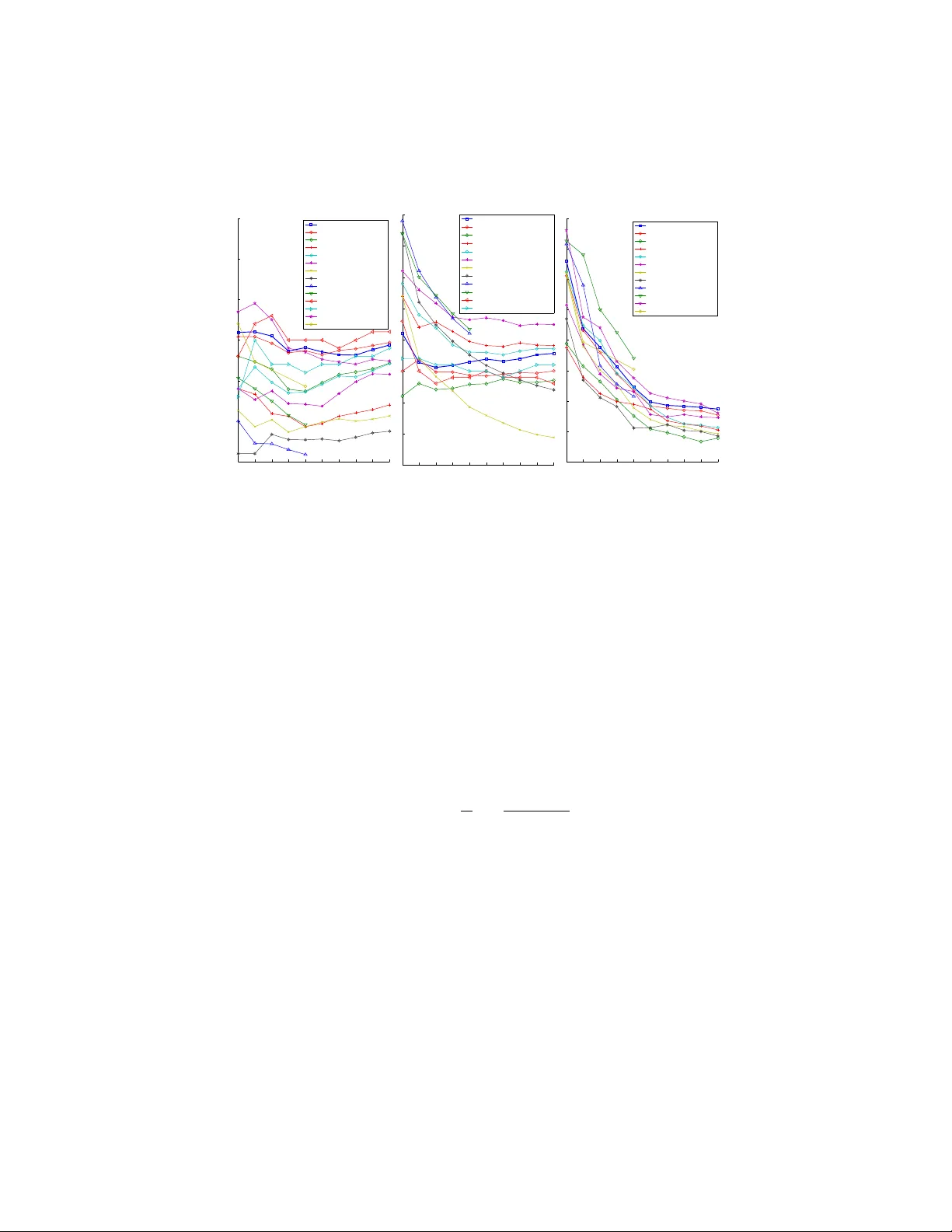
Authors: ** James R. McAllester, Martin J. Wainwright, John D. Lafferty **
Exponential F amily Graph Matching and Ranking James Petterson, T ib ´ erio Caetano, Julian McAuley , Jin Y u ∗ Nov ember 15, 2021 Abstract W e present a method for learning max-weight matching predictors in bipartite graphs. The method consists of performing maximum a posteriori estimation in exponential families with suf ficient statistics that encode permutations and data features. Although inference is in general hard, we show that for one very rele- vant application–web page ranking–e xact inference is efficient. For general model instances, an appropriate sampler is readily av ailable. Contrary to existing max- margin matching models, our approach is statistically consistent and, in addition, experiments with increasing sample sizes indicate superior improvement over such models. W e apply the method to graph matching in computer vision as well as to a standard benchmark dataset for learning web page ranking, in which we obtain state-of-the-art results, in particular improving on max-mar gin variants. The draw- back of this method with respect to max-margin alternativ es is its runtime for large graphs, which is comparativ ely high. 1 Intr oduction The Maximum-W eight Bipartite Matching Problem (henceforth ‘matching problem’) is a fundamental problem in combinatorial optimization [ 26 ]. This is the problem of finding the ‘heaviest’ perfect match in a weighted bipartite graph. An e xact optimal solution can be found in cubic time by standard methods such as the Hungarian algo- rithm. This problem is of practical interest because it can nicely model real-world applica- tions. For example, in computer vision the crucial problem of finding a correspondence between sets of image features is often modeled as a matching problem [ 2 , 3 ]. Ranking algorithms can be based on a matching frame work [ 19 ], as can clustering algorithms [ 14 , 11 ]. When modeling a problem as one of matching, one central question is the choice of the weight matrix. The problem is that in real applications we typically observe edge featur e vectors , not edge weights. Consider a concrete e xample in computer vision: it ∗ NICT A ’ s Statistical Machine Learning program, Locked Bag 8001, ACT 2601, Australia, and Research School of Information Sciences and Engineering, Australian National Uni versity , A CT 0200, Australia. NICT A is funded by the Australian Government’s Backing Australia’s Ability initiative, and the Australian Research Council’ s ICT Centre of Excellence program. e-mails: first.last@nicta.com.au 1 is dif ficult to tell what the ‘similarity score’ is between two image feature points, but it is straightforward to extract feature v ectors (e.g. SIFT) associated with those points. In this setting, it is natural to ask whether we could parameterize the features, and use labeled matches in order to estimate the parameters such that, gi ven graphs with ‘similar’ features, their resulting max-weight matches are also ‘similar’. This idea of ‘parameterizing algorithms’ and then optimizing for agreement with data is called structur ed estimation [ 31 , 33 ]. [ 31 ] and [ 3 ] describe max-margin structured estimation formalisms for this prob- lem. Max-margin structured estimators are appealing in that they try to minimize the loss that one really cares about (‘structured losses’, of which the Hamming loss is an example). Ho wever structured losses are typically piecewise constant in the parame- ters, which eliminates any hope of using smooth optimization directly . Max-margin estimators instead minimize a surrogate loss which is easier to optimize, namely a con- ve x upper bound on the structured loss [ 33 ]. In practice the results are often good, but known con ve x relaxations produce estimators which are statistically inconsistent [ 22 ], i.e., the algorithm in general fails to obtain the best attainable model in the limit of infinite training data. The inconsistency of multiclass support vector machines is a well-known issue in the literature that has receiv ed careful examination recently [ 8 , 7 ]. Motiv ated by the inconsistency issues of max-margin structured estimators as well as by the well-kno wn benefits of ha ving a full probabilistic model, in this paper we present a maximum a posteriori (MAP) estimator for the matching problem. The ob- served data are the edge feature vectors and the labeled matches provided for training. W e then maximize the conditional posterior likelihood of matches gi ven the observed data. W e b uild an exponential f amily model where the sufficient statistics are such that the mode of the distribution (the prediction) is the solution of a max-weight matching problem. The resulting partition function is ] P-complete to compute e xactly . Ho wever , we sho w that for learning to rank applications the model instance is tractable. W e then compare the performance of our model instance ag ainst a large number of state-of-the- art ranking methods, including DORM [ 19 ], an approach that only dif fers to our model instance by using max-margin instead of a MAP formulation. W e show very compet- itiv e results on standard webpage ranking datasets, and in particular we show that our model performs better than or on par with DORM. For intractable model instances, we show that the problem can be approximately solv ed using sampling and we provide experiments from the computer vision domain. Howe ver the fastest suitable sampler is still quite slow for large models, in which case max-margin matching estimators like those of [ 3 ] and [ 31 ] are likely to be preferable e ven in spite of their potential inferior accuracy . 2 2 Backgr ound 2.1 Structured Prediction In recent years, great attention has been dev oted in Machine Learning to so-called structur ed pr edictors , which are predictors of the kind g θ : X 7→ Y , (1) where X is an arbitrary input space and Y is an arbitr ary discrete space, typically expo- nentially lar ge . Y may be, for e xample, a space of matrices, trees, graphs, sequences, strings, matches, etc. This structured nature of Y is what structured pr ediction refers to. In the setting of this paper, X is the set of vector-weighted bipartite graphs (i.e., each edge has a feature vector associated to it), and Y is the set of perfect matches induced by X . If N graphs are av ailable, along with corresponding annotated matches (i.e., a set { ( x n , y n ) } N n =1 ), our task will be to estimate θ such that when we apply the predictor g θ to a ne w graph it produces a match that is similar to matches of similar graphs from the annotated set. Structur ed learning or structur ed estimation refers to the process of estimating a vector θ for predictor g θ when data { ( x 1 , y 1 ) , . . . , ( x N , y N ) } ∈ ( X × Y ) N are av ailable. Structured prediction for input x means computing y = g ( x ; θ ) using the estimated θ . T wo generic estimation strategies have been popular in producing structured predic- tors. One is based on max-margin estimators [ 33 , 32 , 31 ], and the other on maximum- likelihood (ML) or MAP estimators in exponential f amily models [ 18 ]. The first approach is a generalization of support vector machines to the case where the set Y is structured. Howe ver the resulting estimators are known to be inconsistent in general: in the limit of infinite training data the algorithm fails to reco ver the best model in the model class [ 22 , 7 , 8 ]. McAllester recently provided an interesting anal- ysis on this issue, where he proposed ne w upper bounds whose minimization results in consistent estimators, but no such bounds are conv ex [ 22 ]. The other approach uses ML or MAP estimation in conditional exponential families with ‘structured’ sufficient statistics, such as in probabilistic graphical models, where they are decomposed ov er the cliques of the graph (in which case they are called Conditional Random Fields, or CRFs [ 18 ]). In the case of tractable graphical models, dynamic programming can be used to ef ficiently perform inference. Other tractable models of this type include mod- els that predict spanning trees and models that predict binary labelings in planar graphs [ 9 , 17 ]. ML and MAP estimators in exponential families not only amount to solving an unconstrained and con vex optimization problem; in addition they are statistically consistent. The main problem with these types of models is that often the partition function is intractable. This has moti v ated the use of max-margin methods in man y scenarios where such intractability arises. 2.2 The Matching Problem Consider a weighted bipartite graph with m nodes in each part, G = ( V , E , w ) , where V is the set of vertices, E is the set of edges and w : E 7→ R is a set of real-valued weights associated to the edges. G can be simply represented by a matrix ( w ij ) where 3 to attain the grap h G = ( V , E , w ). See Figure 1 for an illustration. G x G i j i j x ij w ij = h x ij , θ i Figure 1. Left: Illustration of an input ve ctor- w eighte d bi- partite graph G x with 3 × 3 edges. There is a v ector x e asso cia ted to eac h edge e (for clarit y only x ij is sho wn, corresp onding to the solid edge). Righ t: w eigh ted bipar- tite graph G obtained b y ev aluating G x on the learned v e ctor θ (again o nly edge ij is sho wn). More formally , assume that a training set { X , Y } = { ( x 1 , y 1 ) , . . . , ( x N , y N ) } is a v ailable, for n = 1 , 2 , . . . , N (where x n := ( x n 11 , x n 12 . . . , x n M ( n ) M ( n ) )). Here M ( n ) i s the n um b er of no des in eac h p art of the v ector-w eigh ted bipartite graph x n . W e then parameterize x ij as w iy ( i ) = f ( x iy ( i ) ; θ ), and the goal is to find the θ whic h maximizes the p osterior lik eliho o d of the observ ed data. W e will assume f to b e bilinear, i.e. f ( x iy ( i ) ; θ ) = x iy ( i ) , θ . 3.2. Exp onen tial F amily M o del W e assume an exp onen tial family mo del, where the probabilit y mo del is p ( y | x ; θ ) = exp ( h φ ( x, y ) , θ i − g ( x ; θ )) , (3) where g ( x ; θ ) = log X y exp h φ ( x, y ) , θ i (4) is the log-partition function, whic h is a con v ex and dif- feren tiable function of θ (W ain wrigh t & Jord an, 2003). The prediction in this mo del is the most lik ely y , i.e. y ∗ = argmax y p ( y | x ; θ ) = argmax y h φ ( x, y ) , θ i (5) and ML estim ati on amoun ts to maximizing the con- ditional lik e l iho o d of a sample { X , Y } , i.e. computing argmax θ p ( Y | X ; θ ). In practice w e will in general in- tro duce a prior on θ and p erform MAP estimation: θ ∗ = argmax θ p ( Y | X ; θ ) p ( θ ) = argma x θ p ( θ | Y , X ) . (6) Assuming iid sampling, w e ha v e p ( Y | X ; θ ) = Q N n =1 p ( y n | x n ; θ ). Therefore, p ( θ | Y , X ) ∝ p ( θ ) N Y n =1 exp ( h φ ( x n , y n ) , θ i − g ( x n ; θ )) = exp log p ( θ ) + N X n =1 ( h φ ( x n , y n ) , θ i − g ( x n ; θ )) ! . (7) W e imp ose a Gaussian prior on θ . Instead of maximiz- ing the p osterior w e can instead minimize the negativ e log-p osterior ` ( Y | X ; θ ), whic h b ecomes our loss func- tion (w e suppress the constan t term): ` ( Y | X ; θ ) = λ 2 k θ k 2 + 1 N N X n =1 ( g ( x n ; θ ) − h φ ( x n , y n ) , θ i ) (8) where λ is a regularization constan t. ` ( Y | X ; θ ) is a con v ex function of θ since the log-partition fu nction g ( θ ) is a con v ex function of θ (W ain wrigh t & Jordan, 2003) and the other terms are clearly con v ex in θ . 3.3. F eature P arameterization The critical observ ation no w is that w e equate th e so- lution of the m atc hing problem (2) to the prediction of the exp onen tial family mo del (5), i.e. P i w iy ( i ) = h φ ( x, y ) , θ i . Si nce our goal is to parameterize fea- tures of individ ual pairs of no des (so as to pro duce the w eigh t of an edge), the most natural mo del is φ ( x, y ) = M X i =1 x iy ( i ) , whic h giv es (9) w iy ( i ) = x iy ( i ) , θ , (10) i.e. linear in b oth x and θ (see Figure 1, righ t). The sp ecific form for x ij will b e discussed in the exp eri- men tal section. In ligh t of (10), (2) no w c l e arl y means a pr e diction of the b est matc h for G x under the mo del θ . 4. Learning the Mo del 4.1. Basics W e need to solv e θ ∗ = argmin θ ` ( Y | X ; θ ). ` ( Y | X ; θ ) is a con v ex and differen tiable function of θ (W ain wrigh t & Jordan, 2003), therefore gradien t descen t will find the global op tim um. In order to compute ∇ θ ` ( Y | X ; θ ), w e need to compute ∇ θ g ( θ ). It is a standard result of exp onen tial families that th e gradien t of the log- partition function is th e exp ectation of the sufficien t statistics: ∇ θ g ( x ; θ ) = E y ∼ p ( y | x ; θ ) [ φ ( x, y )] . (11) Figure 1: Left: Illustration of an input vector-weighted bipartite graph G x with 3 × 3 edges. There is a vector x e associated to each edge e (for clarity only x ij is shown, corresponding to the solid edge). Right: weighted bipartite graph G obtained by e val- uating G x on the learned vector θ (again only edge ij is shown). the entry w ij is the weight of the edge ij . Consider also a bijection y : { 1 , 2 , . . . , m } 7→ { 1 , 2 , . . . , m } , i.e., a permutation. Then the matching problem consists of computing y ∗ = argmax y m X i =1 w iy ( i ) . (2) This is a well-studied problem; it is tractable and can be solv ed in O ( m 3 ) time [ 16 , 26 ]. This model can be used to match features in images [ 3 ], improve classification algo- rithms [ 11 ] and rank webpages [ 19 ], to cite a few applications. The typical setting consists of engineering the score matrix w ij according to domain kno wledge and sub- sequently solving the combinatorial problem. 3 The Model 3.1 Basic Goal In this paper we assume that the weights w ij are instead to be estimated from training data. More precisely , the weight w ij associated to the edge ij in a graph will be the result of an appropriate composition of a featur e vector x ij (observed) and a parameter vector θ (estimated from training data). Therefore, in practice, our input is a vector- weighted bipartite graph G x = ( V , E , x ) ( x : E 7→ R n ), which is ‘ev aluated’ at a particular θ (obtained from previous training) so as to attain the graph G = ( V , E , w ) . See Figure 1 for an illustration. More formally , assume that a training set { X, Y } = { ( x n , y n ) } N n =1 is a vailable, where x n := ( x n 11 , x n 12 . . . , x n M ( n ) M ( n ) ) . Here M ( n ) is the number of nodes in each part of the vector-weighted bipartite graph x n . W e then parameterize x ij as w iy ( i ) = f ( x iy ( i ) ; θ ) , and the goal is to find the θ which maximizes the posterior likelihood of the observed data. W e will assume f to be bilinear , i.e., f ( x iy ( i ) ; θ ) = x iy ( i ) , θ . 4 3.2 Exponential F amily Model W e assume an exponential family model, where the probability model is p ( y | x ; θ ) = exp ( h φ ( x, y ) , θ i − g ( x ; θ )) , where (3) g ( x ; θ ) = log X y exp h φ ( x, y ) , θ i (4) is the log-partition function, which is a con vex and dif ferentiable function of θ [ 35 ]. The prediction in this model is the most likely y , i.e., y ∗ = argmax y p ( y | x ; θ ) = argmax y h φ ( x, y ) , θ i (5) and ML estimation amounts to maximizing the conditional likelihood of the training set { X, Y } , i.e., computing argmax θ p ( Y | X ; θ ) . In practice we will in general introduce a prior on θ and perform MAP estimation: θ ∗ = argmax θ p ( Y | X ; θ ) p ( θ ) = argmax θ p ( θ | Y , X ) . (6) Assuming iid sampling, we hav e p ( Y | X ; θ ) = Q N n =1 p ( y n | x n ; θ ) . Therefore, p ( θ | Y , X ) ∝ p ( θ ) N Y n =1 exp ( h φ ( x n , y n ) , θ i − g ( x n ; θ )) = exp log p ( θ ) + N X n =1 ( h φ ( x n , y n ) , θ i − g ( x n ; θ )) ! . (7) W e impose a Gaussian prior on θ . Instead of maximizing the posterior we can in- stead minimize the negati ve log-posterior ` ( Y | X ; θ ) , which becomes our loss function (we suppress the constant term): ` ( Y | X ; θ ) = λ 2 k θ k 2 + 1 N N X n =1 ( g ( x n ; θ ) − h φ ( x n , y n ) , θ i ) (8) where λ is a re gularization constant. ` ( Y | X ; θ ) is a con vex function of θ since the log- partition function g ( θ ) is a conv ex function of θ [ 35 ] and the other terms are clearly con vex in θ . 3.3 F eatur e Parameterization The critical observation now is that we equate the solution of the matching problem ( 2 ) to the prediction of the exponential family model ( 5 ), i.e., P i w iy ( i ) = h φ ( x, y ) , θ i . 5 Since our goal is to parameterize features of indi vidual pairs of nodes (so as to produce the weight of an edge), the most natural model is φ ( x, y ) = M X i =1 x iy ( i ) , which gives (9) w iy ( i ) = x iy ( i ) , θ , (10) i.e., linear in both x and θ (see Figure 1 , right). The specific form for x ij will be dis- cussed in the e xperimental section. In light of ( 10 ), ( 2 ) no w clearly means a pr ediction of the best match for G x under the model θ . 4 Learning the Model 4.1 Basics W e need to solve θ ∗ = argmin θ ` ( Y | X ; θ ) . ` ( Y | X ; θ ) is a con vex and differentiable function of θ [ 35 ], therefore gradient descent will find the global optimum. In order to compute ∇ θ ` ( Y | X ; θ ) , we need to compute ∇ θ g ( θ ) . It is a standard result of expo- nential families that the gradient of the log-partition function is the expectation of the sufficient statistics: ∇ θ g ( x ; θ ) = E y ∼ p ( y | x ; θ ) [ φ ( x, y )] . (11) Therefore in order to perform gradient descent we need to compute the abo ve expecta- tion. Opening the above e xpression gi ves E y ∼ p ( y | x ; θ ) [ φ ( x, y )] = X y φ ( x, y ) p ( y | x ; θ ) (12) = 1 Z ( x ; θ ) X y φ ( x, y ) M Y i =1 exp( x iy ( i ) , θ ) , (13) which re veals that the partition function Z ( x ; θ ) needs to be computed. The partition function is: Z ( x ; θ ) = X y M Y i =1 exp( x iy ( i ) , θ ) | {z } =: B iy ( i ) . (14) Note that the abo v e is the e xpression for the permanent of matrix B [ 23 ]. The per- manent is similar in definition to the determinant, the difference being that for the latter sgn( y ) comes before the product. Howe ver , unlike the determinant, which is computable efficiently and e xactly by standard linear algebra manipulations [ 17 ], com- puting the permanent is a ] P-complete problem [ 34 ]. Therefore we hav e no realistic hope of computing ( 11 ) exactly for general problems. 6 4.2 Exact Expectation The exact partition function itself can be ef ficiently computed for up to about M = 30 using the O ( M 2 M ) algorithm by Ryser [ 29 ]. Ho we ver for arbitrary expectations we are not aware of any exact algorithm which is more efficient than full enumeration (which w ould constrain tractability to v ery small graphs). Ho wever we will see that ev en in the case of very small graphs we find a very important application: learning to rank. In our e xperiments, we successfully apply a tractable instance of our model to benchmark webpage ranking datasets, obtaining very competiti ve results. For lar ger graphs, we hav e alternati ve options as indicated belo w . 4.3 A ppr oximate Expectation If we hav e a situation in which the set of feasible permutations is too large to be fully enumerated ef ficiently , we need to resort to some approximation for the expectation of the suf ficient statistics. The best solution we are aware of is one by Huber and Law , who recently presented an algorithm to approximate the permanent of dense non-negati ve matrices [ 13 ]. The algorithm works by producing exact samples from the distribution of perfect matches on weighted bipartite graphs. This is in precisely the same form as the distribution we hav e here, p ( y | x ; θ ) [ 13 ]. W e can use this algorithm for applications that in volv e larger graphs. 1 W e generate K samples from the distribution p ( y | x ; θ ) , and directly approximate ( 12 ) with a Monte Carlo estimate E y ∼ p ( y | x ; θ ) [ φ ( x, y )] ≈ 1 K K X i =1 φ ( x, y i ) . (15) In our experiments, we apply this algorithm to an image matching application. 5 Experiments 5.1 Ranking Here we apply the general matching model introduced in previous sections to the task of learning to r ank . Ranking is a fundamental problem with applications in di verse areas such as document retrie val, recommender systems, product rating and others. W e focus on web page ranking. W e are giv en a set of queries { q k } and, for each query q k , a list of D ( k ) documents { d k 1 , . . . , d k D ( k ) } with corresponding ratings { r k 1 , . . . , r k D ( k ) } (assigned by a human ed- itor), measuring the relev ance de gree of each document with respect to query q k . A rating or rele vance degree is usually a nominal v alue in the list { 1 , . . . , R } , where R is typically between 2 and 5. W e are also given, for ev ery retriev ed document d k i , a joint feature vector ψ k i for that document and the query q k . T raining At training time, we model each query q k as a vector -weighted bipartite graph (Figure 1 ) where the nodes on one side correspond to a subset of cardinality M of 1 The algorithm is described in the appendix. 7 all D ( k ) documents retriev ed by the query , and the nodes on the other side correspond to all possible ranking positions for these documents ( 1 , . . . , M ). The subset itself is chosen randomly , provided at least one exemplar document of e very rating is present. Therefore M must be such that M ≥ R . The process is then repeated in a bootstrap manner: we resample (with replace- ment) from the set of documents { d k 1 , . . . , d k D ( k ) } , M documents at a time (conditioned on the fact that at least one ex emplar of every rating is present, but otherwise randomly). This effecti vely boosts the number of training examples since each query q k ends up being selected many times, each time with a dif ferent subset of M documents from the original set of D ( k ) documents. In the follo wing we drop the query index k to examine a single query . Here we follow the construction used in [ 19 ] to map matching problems to ranking problems (indeed the only difference between our ranking model and that of [ 19 ] is that the y use a max-margin estimator and we use MAP in an e xponential family .) Our edge feature vector x ij will be the product of the feature vector ψ i associated with document i , and a scalar c j (the choice of which will be explained belo w) associated with ranking position j x ij = ψ i c j . (16) ψ i is dataset specific (see details belo w). From ( 10 ) and ( 16 ), we hav e w ij = c j h ψ i , θ i , and training proceeds as explained in Section 4 . T esting At test time, we are giv en a query q and its corresponding list of D associ- ated documents. W e then hav e to solve the prediction problem, i.e., y ∗ = argmax y D X i =1 x iy ( i ) , θ = argmax y D X i =1 c y ( i ) h ψ i , θ i . (17) W e now notice that if the scalar c j = c ( j ) , where c is a non-increasing function of rank position j , then ( 17 ) can be solved simply by sorting the values of h ψ i , θ i in decreasing order . 2 In other words, the matching problem becomes one of r anking the values h ψ i , θ i . Inference in our model is therefore very fast (linear time). 3 In this setting it makes sense to interpret the quantity h ψ i , θ i as a scor e of document d i for query q . This leav es open the question of which non-increasing function c should be used. W e do not solve this problem in this paper , and instead choose a fixed c . In theory it is possible to optimize over c during learning, but in that case the optimization problem w ould no longer be con vex. W e describe the results of our method on LETOR 2.0 [ 20 ], a publicly available benchmark data collection for comparing learning to rank algorithms. It is comprised of three data sets: OHSUMED, TD2003 and TD2004. Data sets OHSUMED contains features e xtracted from query-document pairs in the OHSUMED collection, a subset of MEDLINE, a database of medical publications. It contains 106 queries. For each query there are a number of associated documents, with rele v ance de grees judged by humans on three levels: definitely , possibly or not 2 If r ( v ) denotes the vector of ranks of entries of vector v , then h a, π ( b ) i is maximized by the permutation π ∗ such that r ( a ) = r ( π ∗ ( b )) , a theorem due to Polya, Littlew ood, Hardy and Blackwell [ 30 ]. 3 Sorting the top k items of a list of D items takes O ( k log k + D ) time [ 21 ]. 8 1 2 3 4 5 6 7 8 9 10 0.35 0.4 0.45 0.5 0.55 0.6 0.65 k NDCG TD2004 RankMatch (Our Method), M=2 DORM RankBoost RankSVM FRank ListNet AdaRank−MAP AdaRank−NDCG QBRank IsoRank SortNet 20 hiddens MAP SortNet 20 hiddens P@10 StructRank C−CRF 1 2 3 4 5 6 7 8 9 10 0.2 0.25 0.3 0.35 0.4 0.45 0.5 0.55 k NDCG TD2003 RankMatch (Our Method), M=2 (all) DORM RankBoost RankSVM FRank ListNet AdaRank−MAP AdaRank−NDCG QBRank IsoRank SortNet 10 hiddens MAP SortNet 10 hiddens P@10 1 2 3 4 5 6 7 8 9 10 0.42 0.44 0.46 0.48 0.5 0.52 0.54 0.56 0.58 k NDCG OHSUMED RankMatch (Our Method), M=3 DORM RankBoost RankSVM FRank ListNet AdaRank−MAP AdaRank−NDCG QBRank IsoRank StructRank C−CRF Figure 2: Results of NDCG@k for state-of-the-art methods on TD2004 (left), TD2003 (middle) and OHSUMED (right). This is best viewed in color . r ele vant . Each query-document pair is associated with a 25 dimensional feature vector , ψ i . The total number of query-document pairs is 16,140. TD2003 and TD2004 contain features extracted from the topic distillation tasks of TREC 2003 and TREC 2004, with 50 and 75 queries, respecti vely . Again, for each query there are a number of associated documents, with rele v ance degrees judged by humans, but in this case only two levels are provided: rele vant or not r elevant . Each query-document pair is associated with a 44 dimensional feature vector , ψ i . The total number of query-document pairs is 49,171 for TD2003 and 74,170 for TD2004. All datasets are already partitioned for 5-fold cross-validation. See [ 20 ] for more details. Evaluation Metrics In order to measure the effecti veness of our method we use the normalized discount cumulative gain (NDCG) measure [ 15 ] at rank position k , which is defined as NDCG@k = 1 Z k X j =1 2 r ( j ) − 1 log(1 + j ) , (18) where r ( j ) is the rele v ance of the j th document in the list, and Z is a normalization constant so that a perfect ranking yields an NDCG score of 1 . External Parameters The re gularization constant λ is chosen by 5-fold cross- validation, with the partition pro vided by the LETOR package. All experiments are repeated 5 times to account for the randomness of the sampling of the training data. W e use c ( j ) = M − j on all e xperiments. Optimization T o optimize ( 8 ) we use a standard BFGS Quasi-Ne wton method with a backtracking line search, as described in [ 25 ]. Results For the first experiment training was done on subsets sampled as described abov e, where for each query q k we sampled 0 . 4 · D ( k ) · M subsets, therefore increasing 9 the number of samples linearly with M . For TD2003 we also trained with all possible subsets ( M = 2( all ) in the plots). In Figure 2 we plot the results of our method (named RankMatch), for M = R , compared to those achieved by a number of state-of-the-art methods which ha ve published NDCG scores in at least two of the datasets: RankBoost [ 6 ], RankSVM [ 10 ], FRank [ 5 ], ListNet [ 4 ], AdaRank [ 36 ], QBRank [ 38 ], IsoRank [ 37 ], SortNet [ 28 ], StructRank [ 12 ] and C-CRF [ 27 ]. W e also included a plot of our implementation of DORM [ 19 ], using pr ecisely the same resampling methodology and data for a fair comparison. RankMatch performs among the best methods on both TD2004 and OHSUMED, while on TD2003 it performs poorly (for lo w k ) or f airly well (for high k ). W e notice that there are four methods which only report results in two of the three datasets: the tw o SortNet versions are only reported on TD2003 and TD2004, while StructRank and C-CRF are only reported on TD2004 and OHSUMED. RankMatch compares similarly with SortNet and StructRank on TD2004, similarly to C-CRF and StructRank on OHSUMED and similarly to the two versions of SortNet on TD2003. This exhausts all the comparisons against the methods which hav e results reported in only two datasets. A fairer comparison could be made if these methods had their performance published for the respectiv e missing dataset. When compared to the methods which report results in all datasets, RankMatch entirely dominates their performance on TD2004 and is second only to IsoRank on OHSUMED (and performing similarly to QBRank). These results should be interpreted cautiously; [ 24 ] presents an interesting discus- sion about issues with these datasets. Also, benchmarking of ranking algorithms is still in its infanc y and we don’t yet ha ve publicly av ailable code for all of the competitiv e methods. W e expect this situation to change in the near future so that we are able to compare them on a fair and transparent basis. Consistency In a second experiment we trained RankMatch with different training subset sizes, starting with 0 . 03 · D ( k ) · M and going up to 1 . 0 · D ( k ) · M . Once again, we repeated the experiments with DORM using pr ecisely the same training subsets. The purpose here is to see whether we observe a practical advantage of our method with increasing sample size, since statistical consistency only provides an asymptotic indication. The results are plotted in Figure 3 -right, where we can see that, as more training data is av ailable, RankMatch improves more saliently than DORM. Runtime The runtime of our algorithm is competitiv e with that of max-margin for small graphs, such as those that arise from the ranking application. For larger graphs, the use of the sampling algorithm will result in much slower runtimes than those typically obtained in the max-margin framew ork. This is certainly the benefit of the max-mar gin matching formulations of [ 3 , 19 ]: it is much faster for lar ge graphs. T able 1 shows the runtimes for graphs of dif ferent sizes, both for exponential family and max-margin matching models. 10 T able 1: Training times (per observ ation, in seconds) for the exponential model and max-margin. Runtimes for M = 3 , 4 , 5 are from the ranking e xperiments, computed by full enumeration; M = 20 corresponds to the image matching experiments, which use the sampler from [ 13 ]. A problem of size 20 cannot be practically solved by full enumeration. M exponential model max mar gin 3 0.0006661 0.0008965 4 0.0011277 0.0016086 5 0.0030187 0.0015328 20 36.0300000 0.9334556 5.2 Image Matching For our computer vision application we used a silhouette image from the Mythologi- cal Creatures 2D database 4 . W e randomly selected 20 points on the silhouette as our interest points and applied shear to the image creating 200 different images. W e then randomly selected N pairs of images for training, N for validation and 500 for testing, and trained our model to match the interest points in the pairs. In this setup, x ij = | ψ i − ψ j | 2 , (19) where | · | denotes the elementwise difference and ψ i is the Shape Context feature v ector [ 1 ] for point i . For a graph of this size computing the exact expectation is not feasible, so we used the sampling method described in Section 4.3 . Once again, the regularization constant λ was chosen by cross-validation. Gi ven the fact that the MAP estimator is consistent while the max-mar gin estimator is not, one is tempted to in vestigate the practical performance of both estimators as the sample size grows. Howe ver , since consistency is only an asymptotic property , and also since the Hamming loss is not the criterion optimized by either estimator , this does not imply a better lar ge-sample performance of MAP in real experiments. In any case, we present results with varying training set sizes in Figure 3 -left. The max-margin method is that of [ 3 ]. After a sufficiently lar ge training set size, our model seems to enjoy a slight advantage. 6 Conclusion and Discussion W e presented a method for learning max-weight bipartite matching predictors, and ap- plied it e xtensi vely to well-kno wn webpage ranking datasets, obtaining state-of-the-art results. W e also illustrated–with an image matching application–that larger problems can also be solv ed, albeit slowly , with a recently de veloped sampler . The method has a number of conv enient features. First, it consists of performing maximum-a-posteriori estimation in an exponential family model, which results in a simple unconstrained con vex optimization problem solvable by standard algorithms such as BFGS. Second, 4 http://tosca.cs.technion.ac.il 11 0 50 100 150 200 250 300 350 400 450 500 0.08 0.1 0.12 0.14 0.16 0.18 0.2 number of training pairs error exponential model max margin gro ws. Ho we v er , since consistenc y is only an asymptotic property , and also since the Hamming loss is not the criterion optimized by either estimator , this does not imply a better lar ge-sample performance of MAP in real e xperiments. In an y case, we present results with v arying training set sizes in Figure 2. In Figure ?? we can see an e xample of a match with and without learning. The max-mar gin method is that of [ ? ]. The methods perform almost identically after a suf ficiently lar ge training set size, although the e xperiment w as truncated at 500 training/testing pairs due to computational o v erload. (The dataset has in total about 20,000 dif ferent image pairs.) 0 50 100 150 200 250 300 350 400 450 500 0.08 0.1 0.12 0.14 0.16 0.18 0.2 number of training pairs error max margin exponential model Figure 3: Left: match without learning (6/20 correct matches). Right: match with learning (14/20 correct matches) and training of θ proceeds as e xplained in Section 4. T esting At test time, we are gi v en a query q and its corresponding list of D associated documents. W e then ha v e to solv e the prediction problem, i.e. y ∗ = argmax y D X i =1 x iy ( i ) , θ (19a) = argmax y D X i =1 c y ( i ) h ψ i , θ i . (19b) W e no w notice that if the scalar c j = c ( j ) , where c is a non-increasing function of rank pos ition j , then (19b) can be solv ed simply by sorting the v alues of h ψ i , θ i in decreasing order . 3 In other w ords, the matching problem becomes one of r anking the values h ψ i , θ i . Inference in our model is therefore v ery f ast (linear time). 4 In this setti n g it mak es sense to interpret the quantity h ψ i , θ i as a scor e of document d i for query q . This lea v es open the question of which non-increasing function c should be used. W e do not solv e this problem in this paper , and instead choose a fix ed c . In theory it is possible to optimize o v er c during learning, b ut in that case the optimization problem w ould no longer be con v e x. W e descri be the results of our method on LET OR 2.0 [22], a publicly a v ailable benchmark data collection for comparing learning to rank algorithms. It is comprised of three data sets: OHSUMED, TD2003 and TD2004. Data sets OHSUMED contains feat ures e xtracted from query-document pairs in the OHSUMED collection, a subset of MEDLINE, a database of medical publications. It contains 106 queries. F or each query there are a number of associated documents, with rele v a nce de grees judged by humans on three le v els: definitely , possibly or not r ele vant . Each query-document pair has a 25 dimensi onal feature v ector associated (our ψ i ). The total number of query-document pairs is 16,140. TD2003 and TD2004 contain features e xtracted from the topic distillation tasks of TREC 2003 and TREC 2004, with 50 and 75 queries respecti v ely . Ag ain, for each query there are a number of associated documents, with rele v ance de grees judged by humans, b ut in this case only t w o le v els are pro vided: r ele vant or not r ele vant . Each query-document pair has a 44 dimensional feature v ector associated (our ψ i ). The total number of query-document pairs is 49,171 for TD2003 and 74,170 for TD2004. All datasets are already partitioned for 5-fold cross-v alidation. See [22] for more detail. Ev aluation Metrics In order to measure the ef fecti v eness of our method we use the normalized discount cumulative gain (NDCG) measure [16] at rank position k , which is defined as NDCG@k = 1 Z k X j =1 2 r ( j ) − 1 log (1 + j ) , (20) where r ( j ) is the rele v ance of the j th document in the list, and Z is a normalization constant so that a perfect ranking yields an NDCG score of 1 . 3 If r ( v ) denotes the v ector of ranks of entries of v ector v , then h a, π ( b ) i is maximized by the pe rmutation π ∗ such that r ( a ) = r ( π ∗ ( b )) , a theorem due to Polya, Little w ood, Hardy and Blackwell [31]. 4 Sorting the top k items of a list of D items tak es O ( k log k + D ) time with a quicksort-style agorithm. 7 Figure 2: Learning image matching: hamming loss for dif ferent number of training pairs (test set size fix ed to 500 pairs). 5.2 Ranking Here we apply the general matching model introduced in pre vious sections to the task of learning to r ank . Ranking is a fundamental problem with applications in di v erse areas such as document retrie v al, recommender s ystems, product rating and others. W e are going to focus on web page ranking. F or t his problem we are gi v en a set of queries { q k } and, for each query q k , a list of D ( k ) documents { d k 1 , . . . , d k D ( k ) } with corresponding ratings { r k 1 , . . . , r k D ( k ) } (assigned by a human editor), measur - ing the rele v ance de gree of each document with respect to query q k . A rat ing or rele v ance de gree is usually a nominal v alue in the list { 1 , . . . , R } , where R is typically between 2 and 5. W e are also gi v en, for e v ery retrie v ed document d k i , a joint feature v ector ψ k i for that document and the query q k . T raining At training time, we model each query q k as a v ector -weighted bipartite graph (Figure 1) where the nodes on one side correspond to a subset of cardinality M of all D ( k ) documents retrie v ed by the query , and the nodes on the other side correspond to all possible ranking positions for these documents ( 1 , . . . , M ). The subset itself is chosen randomly , pro vided at least one e x emplar document of e v ery rating is present. Therefore M must be such that M ≥ R . The process is then repeated in a bootstrap manner: we resample (with repl acement) from the set of documents { d k 1 , . . . , d k D ( k ) } , M documents at a time (conditioned on the f act that at least one 6 10 −1 10 0 0.53 0.535 0.54 0.545 0.55 0.555 0.56 0.565 0.57 sample size (x M D) NDCG−1 OHSUMED RankMatch DORM Figure 2: Learning image matching. Left: hamming loss for dif ferent numbers of training pairs (test set size fix ed to 500 pairs). Right: an e xample match from the test set (blue are correct and red incorrect matches). retrie v al, recommender s ystems, product rating and others. W e are going to focus on web page ranking. F or t his problem we are gi v en a set of queries { q k } and, for each query q k , a list of D ( k ) documents { d k 1 , . . . , d k D ( k ) } with corresponding ratings { r k 1 , . . . , r k D ( k ) } (assigned by a human editor), measur - ing the rele v ance de gree of each document with respect to query q k . A rat ing or rele v ance de gree is usually a nominal v alue in the list { 1 , . . . , R } , where R is typically between 2 and 5. W e are also gi v en, for e v ery retrie v ed document d k i , a joint feature v ector ψ k i for that document and the query q k . T raining At training time, we model each query q k as a v ector -weighted bipartite graph (Figure 1) where the nodes on one side correspond to a subset of cardinality M of all D ( k ) documents retrie v ed by the query , and the nodes on the other side correspond to all possible ranking positions for these documents ( 1 , . . . , M ). The subset itself is chosen randomly , pro vided at least one e x emplar document of e v ery rating is present. Therefore M must be such that M ≥ R . The process is then repeated in a bootstrap manner: we resample (with repl acement) from the set of documents { d k 1 , . . . , d k D ( k ) } , M documents at a time (conditioned on the f act that at least one e x emplar of e v ery rating is present, b ut otherwise randomly). This ef fecti v ely boosts the number of training e xamples since each query q k ends up being selec ted man y times, each time with a dif ferent subset of M documents from the original set of D ( k ) documents. In the follo wing we drop the query inde x k since we e xamine a single query . Here we follo w the construction used in [21] to map matching problems to ranking problems. (Indeed the only dif ference between our ranking model and that of [21] is that the y use a max-mar gin estima tor and we use MAP in an e xponential f amily .) Our edge feature v ector x ij will be the product of feature v ector ψ i associated with docume nt i , and a scalar c j (the choice of which will be e xplained belo w) associated with ranking position j x ij = ψ i c j . (17) ψ i is dataset specific (details belo w). W e therefore ha v e from (10) and (17) that w ij = c j h ψ i , θ i , (18) and training of θ proceeds as e xplained in Section 4. 6 Figure 3: Performance with increasing sample size. Left: hamming loss for different numbers of training pairs in the image matching problem (test set size fixed to 500 pairs). Right: results of NDCG@1 on the ranking dataset OHSUMED. This evidence is in agreement with the fact that our estimator is consistent, while max-mar gin is not. the estimator is not only statistically consistent but also in practice it seems to benefit more from increasing sample sizes than its max-margin alternativ e. Finally , being fully probabilistic, the model can be easily integrated as a module in a Bayesian frame work, for example. The main direction for future research consists of finding more efficient ways to solve large problems. This will most lik ely arise from appropriate e xploitation of data sparsity in the permutation group. Refer ences [1] Belongie, S., & Malik, J (2000). Matching with shape contexts. CBAIVL00 . 11 [2] Belongie, S., Malik, J., & Puzicha, J. (2002). Shape matching and object recogni- tion using shape contexts. IEEE T rans. on P AMI , 24 , 509–521. 1 [3] Caetano, T . S., Cheng, L., Le, Q. V ., & Smola, A. J. (2009). Learning graph matching. IEEE T rans. on P AMI , 31 , 1048–1058. 1 , 2 , 4 , 10 , 11 [4] Cao, Z., Qin, T ., Liu, T .-Y ., Tsai, M.-F ., & Li, H. (2007). Learning to rank: from pairwise approach to listwise approach. ICML 10 [5] Tsai, M., Liu, T ., Qin, T ., Chen, H., & Ma, W . (2007). Frank: A ranking method with fidelity loss. SIGIR . 10 [6] Freund, Y ., Iyer , R., Schapire, R. E., & Singer , Y . (2003). An ef ficient boosting algorithm for combining preferences. J. Mac h. Learn. Res. , 4 , 933–969. 10 [7] Liu, Y . & Shen, X. (2006) Multicategory ψ -learning. JASA , 101 , 500–509. 2 , 3 [8] Liu, Y . & Shen, X. (2005) Multicategory ψ -learning and support vector machine: Computational tools. J. Computational and Gr aphical Statistics , 14 , 219–236. 2 , 3 12 [9] Globerson, A., & Jaakkola, T . (2007). Approximate inference using planar graph decomposition. NIPS . 3 [10] Herbrich, A., Graepel, T ., & Obermayer , K. (2000). Large margin rank bound- aries for ordinal regression. In Advances in Lar ge Margin Classifier s . 10 [11] Huang, B., & Jebara, T . (2007). Loopy belief propagation for bipartite maximum weight b-matching. AIST A TS . 1 , 4 [12] Huang, J. C., & Frey , B. J. (2008). Structured ranking learning using cumulativ e distribution netw orks. In NIPS . 10 [13] Huber , M., & Law , J. (2008). Fast approximation of the permanent for very dense problems. SODA . 7 , 11 , 14 , 15 [14] Jebara, T ., & Shchogole v , V . (2006). B-matching for spectral clustering. ECML . 1 [15] Jarvelin, K., & Kekalainen, J. (2002). Cumulated gain-based ev aluation of ir techniques. ACM T ransactions on Information Systems , 20 , 2002. 9 [16] Jonker , R., & V olgenant, A. (1987). A shortest augmenting path algorithm for dense and sparse linear assignment problems. Computing , 38 , 325–340. 4 [17] K oo, T ., Globerson, A., Carreras, X., & Collins, M. (2007). Structured prediction models via the matrix-tree theorem. EMNLP . 3 , 6 [18] Lafferty , J. D., McCallum, A., & Pereira, F . (2001). Conditional random fields: Probabilistic modeling for segmenting and labeling sequence data. ICML . 3 [19] Le, Q., & Smola, A. (2007). Direct optimization of ranking measures. http://arxiv .org/abs/0704.3359. 1 , 2 , 4 , 8 , 10 [20] Liu, T .-Y ., Xu, J., Qin, T ., Xiong, W ., & Li, H. (2007). Letor: Benchmark dataset for research on learning to rank for information retriev al. LR4IR . 8 , 9 [21] Martinez, C. (2004). Partial quicksort. SIAM . 8 [22] McAllester , D. (2007). Generalization bounds and consistency for structured la- beling. Predicting Structur ed Data . 2 , 3 [23] Minc, H. (1978). P ermanents . Addison-W esley . 6 [24] Minka, T ., & Robertson, S. (2008). Selection bias in the letor datasets. LR4IR . 10 [25] Nocedal, J., & Wright, S. J. (1999). Numerical optimization . Springer Series in Operations Research. Springer . 9 [26] Papadimitriou, C. H., & Steiglitz, K. (1982). Combinatorial optimization: Algo- rithms and complexity . Ne w Jersey: Prentice-Hall. 1 , 4 13 [27] Qin, T ., Liu, T .-Y ., Zhang, X.-D., W ang, D.-S., & Li, H. (2009). Global ranking using continuous conditional random fields. NIPS . 10 [28] Rigutini, L., Papini, T ., Maggini, M., & Scarselli, F . (2008). Sortnet: Learning to rank by a neural-based sorting algorithm. LR4IR . 10 [29] Ryser , H. J. (1963). Combinatorial mathematics . The Carus Mathematical Mono- graphs, No. 14, Mathematical Association of America. 7 [30] Sherman, S. (1951). On a Theorem of Hardy , Little wood, Polya, and Blackwell. Pr oceedings of the National Academy of Sciences , 37 , 826–831. 8 [31] T askar, B. (2004). Learning structured prediction models: a lar ge-mar gin ap- pr oach . Doctoral dissertation, Stanford University . 2 , 3 [32] T askar, B., Guestrin, C., & K oller , D. (2004). Max-margin Marko v networks. NIPS 3 [33] Tsochantaridis, I., Joachims, T ., Hofmann, T ., & Altun, Y . (2005). Large margin methods for structured and interdependent output v ariables. JMLR , 6 , 1453–1484. 2 , 3 [34] V aliant, L. G. (1979). The complexity of computing the permanent. Theor . Com- put. Sci. (pp. 189–201). 6 [35] W ainwright, M. J., & Jordan, M. I. (2003). Graphical models, exponential fam- ilies, and variational infer ence (T echnical Report 649). UC Berkele y , Department of Statistics. 5 , 6 [36] Xu, J., & Li, H. (2007). Adarank: a boosting algorithm for information retriev al. SIGIR . 10 [37] Zheng, Z., Zha, H., & Sun, G. (2008a). Query-le vel learning to rank using isotonic regression. LR4IR . 10 [38] Zheng, Z., Zha, H., Zhang, T ., Chapelle, O., Chen, K., & Sun, G. (2008b). A general boosting method and its application to learning ranking functions for web search. NIPS . 10 A ppendix A For completeness we include a description of the sampling algorithm presented in [ 13 ]. The algorithm is an accept-reject algorithm. The core idea of such an algorithm is very simple: assume we need to sample from a distribution p in a gi ven domain M , b ut that such a task is intractable. Instead, we sample from a distribution q in a superset N of the original domain (in which sampling is easier), whose restriction to the original domain coincides with the original distribution: q | N = p . W e then only ‘accept’ those samples that ef fecti vely fall within the original domain M . Clearly , the ef ficiency of such a procedure will be dictated by (i) how efficient it is to sample from q in N and 14 (ii) how much mass of q is in M . Roughly speaking, the algorithm presented in [ 13 ] manages to sample perfect matches of bipartite graphs such that both conditions (i) and (ii) are fa vorable. The reasoning goes as follows: the problem consists of generating variates y ∈ Y ( y is a match) with the property that p ( y ) = w ( y ) / Z , where w ( y ) is the non- negati ve score of match y and Z = P y w ( y ) is the partition function, which in our case is a permanent as discussed in Section 4.1. W e first partition the space Y into Y 1 , . . . , Y I , where Y i = { y : y (1) = i } . Each part has its own partition function Z i = P y ∈ Y i w ( y ) . Next, a suitable upper bound U ( Y i ) ≥ Z i on the partition function is constructed such that the following tw o properties hold: 5 (P1) M X i =1 U ( Y i ) ≤ U ( Y ) . (P2) If | Y i | = 1 , then U ( Y i ) = Z i = w ( y ) . That is, (i) the upper bound is super-additi ve in the elements of the partition and (ii) if Y i has a single match, the upper bound equals the partition function, which in this case is just the score of that match. Now the algorithm: consider the random variable I where p ( I = i ) = U ( Y i ) /U ( Y ) . By (P1), P M i =1 p ( i ) ≤ 1 , so assume p ( I = 0) = 1 − P M i =1 p ( i ) . Now , draw a variate from this distrib ution, and if I = i = 0 , reject and restart, otherwise recursi vely sample in Y i . 6 This algorithm either stops and restarts or it reaches Y final which consists of a match, i.e., | Y final | = 1 . This match is then a legitimate sample from p ( y ) . The reason this is the case is because of (P2), as sho wn below . Assuming the algorithm finishes after k samples, the probability of the match is the telescopic product U ( Y I (1) ) U ( Y ) U ( Y I (2) ) U ( Y I (1) ) . . . U ( Y I ( k ) ) U ( Y I ( k − 1) ) ( P 2) = w ( y ) U ( Y ) , (20) and since the probability of acceptance is Z/U ( Y ) , we hav e p ( y ) = w ( y ) /U ( Y ) Z/U ( Y ) = w ( y ) Z , (21) which is indeed the distribution from which we want to sample. For pseudocode and a rigorous presentation of the algorithm, see [ 13 ]. 5 See [ 13 ] for details. 6 Due to the self-reducibility of permutations, when we fix y (1) = i , what remains is also a set of permutations. W e then sample y (2) , y (3) . . . y ( M ) . 15
Original Paper
Loading high-quality paper...
Comments & Academic Discussion
Loading comments...
Leave a Comment