Adaptive design and analysis of supercomputer experiments

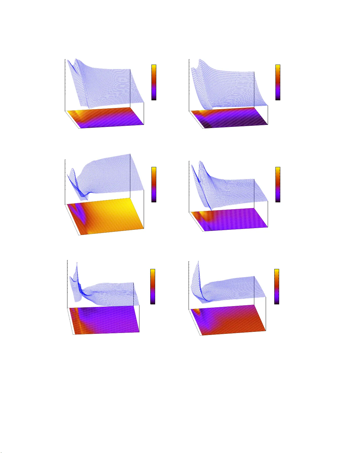
Adaptiv e design and analysis of sup ercomputer exp erimen ts Rob ert B. Gra macy bobb y@stats lab.cam.ac.uk Stati stical Lab orato ry Universit y of Cambridge Herb ert K. H. Lee herb ie@ams. ucsc.edu Dept of Appli ed Math & Sta tistics Universit y of Cal ifornia, Santa Cruz Abstract Computer exp erimen ts are often p erformed to allo w mo deling of a resp onse surface of a physic al exp erimen t that ca n b e too costly or diﬃcult to run except using a sim ulator. Runnin g the exp erimen t o ver a dens e grid can b e prohibitiv ely exp ensiv e, ye t run ning o v er a sp ars e design c hosen in adv ance can result in insuﬃcient information in parts of the sp a ce, particularly wh en the s urface calls for a nonstationary mo del. W e prop ose an approac h that automatically explores the sp ac e while sim ultaneously ﬁtting the resp onse su rface, using predictive u n ce r ta int y to guide subsequ ent exp erimen tal ru n s. The newly deve lop ed Ba yesian treed Gaussian pro cess is used as the su rrogat e mo del, and a fully Bay esian approac h allo ws explicit measur es of uncertaint y . W e develo p an adaptiv e sequential d e sign framework to cop e with an async hr onous, rand om, agen t– based sup ercomputing en vironment, by using a hybrid appr o ach that melds optimal strategies fr om the statistics literature with ﬂ exible strategies f rom the activ e learning literature. The merits of this ap p roac h are b orne out in sev eral examples, including the motiv ating computational ﬂ u id dyn amic s sim u la tion of a ro c k et b o oster. Key words: nonstationary spatial mo del, treed partitioning, sequentia l design, activ e learning 1 1 In tro duc tion Man y complex phenomena are diﬃcult to in v estigate d irectly through con trolled exp eri- men ts. Instead, computer sim ulatio n is b ecoming a commonplace alternative t o provide insigh t into suc h phenomena (Sac ks et a l., 198 9; Santner et al., 2 003). How ev er, the drive to wards higher ﬁdelit y sim ulat io n contin ues to tax the fa ste st computers, ev en in highly distributed computing environme nts. Computational ﬂuid dynamics (CFD) sim ulations in whic h ﬂuid ﬂo w phenomena are mo deled are an excellen t example—ﬂuid ﬂows ov er complex surfaces ma y b e mo deled accurately but o nly at the cost o f sup ercomputer resources. In this pap er w e explore the problem of ﬁtting a resp onse surface for a computer mo del when the exp eriment can b e designed ada pt ively , i.e., online—a task to whic h the Bay esian ap- proac h is particularly w ell–suited. T o do so, w e will com bine elemen ts from treed mo deling (Chipman et al., 2002) with mo dern Ba ye sian surrog a te mo deling (Kennedy and O’Ha g an, 2001), and elemen ts of the sequen tial design of computer exp erime nts (Santne r et al., 2003) with a ctiv e learning (MacKa y, 1992; Cohn, 1996). The result is a fast and ﬂexible design in terface for t he sequen tial design of sup ercomputer experiments . Consider a sim ulation mo del whic h deﬁnes a mapping, p erhaps non-deterministic, from parameters describing the inputs to one or more output resp onses. Without an analytic represen tation of this mapping, sim ulations must b e run for man y diﬀerent input conﬁgu- rations in order to build up an understanding of its p ossible outcomes. Ev en in extremely parallel computing en vironmen ts, computational exp ens e of the sim ulation and/or high di- mensional input o ften prohibits the na ¨ ıv e approac h o f running the exp erime nt ov er a dense grid of input conﬁgura t io ns . More sophisticated design strategies, such as a Latin Hyp ercub e sample (LHS), ma ximin designs, orthogonal arr a ys, and maxim um en tropy designs can o ﬀ e r an impro v emen t ov er gridding. Seq uential v ersions o f these are b etter still. Ho w ev er, suc h traditional approach es are “stationary” (or global, or uniform) in t he sense they a re based on a metric (e.g., distance) whic h is measured identic ally t hr o ughout the input space. The 2 resulting designs are sometimes called “ s par s e”, or “space-ﬁlling”. Maxim um en trop y designs are literally stationary when ba sed on stationary mo dels (e.g., linear or Gaussian Process mo dels). Suc h sparse, or stationary , design strategies a re a mismatc h when the resp onses necessitate a nonstationary mo del—common in exp erimen ts mo deling phy sical pro cess es, e.g., ﬂuid dynamics—as they cannot learn ab out, and th us concen trate exploration in, more in teresting or complicated regions of the input space. F or example, NASA is dev eloping a new re-usable ro c k et b o oster called the Langley Glide–Bac k Bo oster (LGBB). Muc h of it s dev elopmen t is b eing done with computer mo d- els. In part icular, NASA is inte rested in learning a b out the resp onse in ﬂight c haracteristics (lift, drag, pitc h, side–force, ya w, and roll) of the LGBB as a function of three inputs (sp eed in Mac h num ber, angle of attac k, and side slip angle) when the v ehicle is re- en tering the atmosphere. F or eac h input conﬁgurat ion triplet, CFD sim ulations yield six resp onse out- puts. Figure 1 sho ws the lift resp onse a s a function of speed (Mac h) and angle of at t ac k X[2]=Mach X[1]=alpha Z=lift 1 2 3 4 5 6 −5 0 5 10 15 20 25 30 CDF Data, Beta=0 mach alpha Figure 1 : Lift plo tted a s a function of Mac h (sp eed) and alpha (angle of attack) with b eta (side-slip angle) ﬁxed to zero. The ridge at Mac h 1 separates subsonic from sup ersonic cases. (alpha) with the side-slip angle (b eta) ﬁxed at zero. The ﬁgure shows how the c har a cte ristics 3 of subsonic ﬂow s can b e quite diﬀerent from sup ersonic ﬂo ws, as indicated by the ridge in the resp onse surface at Mach 1. Moreo v er, the transition b et w een subsonic and sup ersonic is distinctly non-linear and ma y ev en b e non-diﬀeren tiable or non-con tinuous. The CFD sim ulations inv olv e the iterative integration o f invis cid Euler equations and are thus com- putationally demanding. Eac h run of the Euler solv er for a given set of para me ters tak es on the order of 5–2 0 hours on a high end w orkstation. Since sim ulation is expensiv e, there is inte rest in b eing a ble to auto matically a nd a daptiv ely design t he exp erimen t to learn ab out where resp onse is most in teresting, e.g., where uncertaint y is la r ges t o r the structure is ric hest, and sp end relatively more eﬀort sampling in these areas. How ev er, b efore a clev er sequen tial design strategy can b e devised, a nonstationary mo del is needed that can capture the diﬀerences in b eha vior b et w een subsonic and sup ersonic ph ysical regimes. The surrogate mo del commonly used to approximate outputs to computer exp erimen ts is the Gaussian pro cess (GP) (Santne r et al., 2003). The GP is conceptually straigh tfor - w ard, easily accommo dates prior kno wledge in the for m of cov a riance functions, and returns estimates of predictiv e conﬁdence. In spite of its simplicit y , there are t w o imp ortan t disad- v an tages to the standard G P in this setting. Firstly , the computation time for inference on the G P scales po orly with the n um b er of data p oin ts, t ypically gro wing with the cube of the sample size. But mo st imp ortantly , G P mo dels are usually stationary in that the same co v ariance structure is used througho ut the en tire input space. In the application of high– v elo cit y computational ﬂuid dynamics, where subsonic ﬂow is quite diﬀeren t from sup ersonic ﬂo w, this limitation is unacceptable. Therefore, the error (standard deviation) asso ciated with a predicted resp onse under a GP mo del do es not lo cally dep end on an y of the previously observ ed output resp onses. The Bay esian tr eed GP mo del (Gra macy and Lee, 20 0 8a) w as designed to o v ercome these limitations. Ideally , we w ould lik e to b e able to com bine the treed GP mo del with classic mo del–based optimal de sign algo rithms. How ev er, classic design algorithms are ill–suited to partition mo d- 4 els and Bay esian Mon te Carlo–ba s ed inference. They ar e inheren tly serial and th us tacitly assume a controlled and isolated computing en vironmen t. The mo dern sup ercomputer has thousands of computing no des, or agents, designed to serv e a mu ltit ude of div erse users. If the design strategy is not prepared to engage a n agent as so on as it b ecomes a v ailable, then that resource is either w asted or dev oted to another pro cess. If design is to b e sequen tial (whic h it m ust, in order to learn ab out the r es p onses online, and adapt the mo del), then the in terface m ust b e async hronous, and an y computation m ust execute in parallel. There ma y not b e time to re-ﬁt the mo del a nd compute the next optimal design. So the ﬁnal ingredients in our ﬂexible design framew ork are a ctive learning strategies from t he Mac hine Learning literature. Such strategies hav e b een used as fast, Monte Carlo–friendly , approx imate alter- nativ es to optimal sequen tial design (Seo et al., 2000). Th us this pap er makes t wo primary contributions: an integrated sequen tial design strat - egy for a mo dern nonstationary mo del, and metho ds for designing exp erimen ts in an asyn- c hronous parallel computing en vironmen t. Our hy brid design strategy puts tog ethe r the treed GP mo del, classic sequen tial design, and activ e learning, resulting in a highly eﬃcien t non- stationary mo del and sequen tial design com bination t ha t balances optimality and ﬂexibility . The r emainder o f this pa p er is organized as fo llo ws. Section 2 reviews the main ingredien ts: from con v entional optimal designs and activ e learning strategies with the canonical station- ary GP mo del, to the nonstationary treed GP mo del with Bay esian mo del av eraging and h ybrid sequen tial design. Section 3 details our approach to the sequen tial design of sup er- computer experiments with the treed GP surrogate mo del. Illustrative examples are giv en on syn thetic data in Section 4. The motiv ating example of a sup ercompute r exp erimen t in- v olving computational ﬂuid dynamics co de for designing a re-usable launc h ve hicle (LGBB) is describ ed in Section 5. Section 6 oﬀers some discussion and a v enue s for further researc h. 5 2 Review Our approach to the adaptiv e design of sup ercomputer exp erimen ts com bines classic design strategies and activ e learning with a modern appro ac h to nonstationary spatial modeling. These topics are review ed here. 2.1 Surrogate Mo deling In a computer experiment, the sim ulation output z ( x ), for a pa rticular (multiv ariat e) input conﬁguration v alue x , is typic ally mo deled as a zero mean random pro cess with cov ar iance C ( x , x ′ ) = σ 2 K ( x , x ′ ). The statio na ry Gaussian pro cess ( G P) is a p opular example of suc h a mo del, and conseque ntly is the canonical surrogate mo del used in designing computer exp eriments (Sacks et al., 1989; Santner et al., 2003). F or data D = { x ⊤ i , z i } N i =1 = { X , Z } o f m X –dimensional inputs X and scalar observ ations Z under a GP mo del, the densit y ov er o utputs at a new p oin t x has a Normal distribution with mean ˆ z ( x ) = k ⊤ ( x ) K − 1 Z , and v ariance ˆ σ 2 ( x ) = σ 2 [ K ( x , x ) − k ⊤ ( x ) K − 1 k ( x )] (1) where k ⊤ ( x ) is the N –v ector whose i th comp onen t is K ( x , x i ), and K is the N × N matrix with i, j elemen t K ( x i , x j ). It is imp ortan t to note that the uncertain t y , ˆ σ 2 ( x ), asso ciated with the prediction has no direct dep enden ce on the nearby observ ed sim ulation outputs Z ; b ecause of t he assumption of stationarity , all resp onse p oin ts contribute to the estimation of the lo cal error through their inﬂuence on the corr elation function K ( · , · ), and the induced correlation matrix K i,j = K ( x i , x j ). W e follow G ramacy and Lee (2008) in sp ecifyin g that K ( · , · ) hav e the fo r m K ( x j , x k | g ) = K ∗ ( x j , x k ) + g δ j,k , (2) 6 where δ · , · is the Kronec ke r delta function, and K ∗ is a true correlation function. The g term, referred to as the nugge t , is p ositiv e ( g > 0) and pro vides a mec hanism for introducing measuremen t error into the sto c hastic pro ces s. It arises when considering a model of the form z ( x ) = w ( x ) + η ( x ) where w ( x ) is the random pro cess with co v ariance C , a nd η ( · ) is indep ende nt Gaussian noise. V alid correlation functions K ∗ ( · , · ) are usually generated as a mem b er o f a parametric family , suc h as the separable p o wer or Mat ´ ern families. A general reference for families o f correlation functions K ∗ is pro vided by Abrahamsen (1997). Hereafter w e use the separable p o w er family , K ∗ ( x j , x k | d ) = exp ( − m X X i =1 | x ij − x ik | p 0 d i ) , (3) whic h is a standard choice in mo deling computer exp erimen ts (Santner et al., 200 3). W e ﬁx p 0 = 2 and infer t he range parameters { d i } m X i =1 as part of our estimation pro cedure. While man y authors (e.g., San tner et al., 20 03; Sac ks et a l., 1989) delib erately omit the n ugget parameter on the grounds tha t computer exp erimen ts are deterministic, w e hav e found it mor e helpful to include a n ugget. Most imp ortan tly , w e found that the L G BB sim u- lator was only t heoretically deterministic, but not necessarily so in practice. Researc hers at NASA explained to us that their n umerical CFD solv ers are t ypically started with random initial v alues, a nd in v olve forced random restarts when diagnostics indicate that con v ergence is p o or. F urthe rmor e, due to the sometimes c haotic b eha vior of the systems, input conﬁgu- rations arbitrarily close to one another can fail to ach ieve the same estimated con v ergence, ev en after satisfying the same stopping criterion. Th us a conv en tional G P mo del without a small–distance noise pro cess (n ugget) can b e a mismatc h to suc h p oten tially non- sm o oth data. As a secondary concern, n umerical stability in decomp osing cov aria nce matrices can b e impro v ed by using a small nugget term (Neal, 1997). 7 2.1.1 T reed Gaussian pro cess mo del Because of concerns ab out the inadequacy of the stationarit y assumption, we prop ose a surrogate mo del tha t is new in the realm of sequen tial design of exp erimen ts: the Ba ye sian treed G auss ia n pro ces s (treed G P) mo del (Gramacy and Lee, 2008a). The treed GP mo del extends the Bay esian treed linear mo del b y using a GP mo del with linear trend independen tly within each region, instead of constant (Chipman et al., 1998; Denison et al., 1 9 98) o r linear (Chipman et al., 2002) mo dels in the partitions. A pro cess prior (Chipman et al., 1998) is placed on the tree T , and conditional on T , parameters for R indep enden t GPs in regions { r ν } R ν =1 are sp eciﬁed via a hierarchic al generativ e mo del: Z ν | β ν , σ 2 ν , K ν ∼ N n ν ( F ν β ν , σ 2 ν K ν ) β 0 ∼ N m ( µ , B ) σ 2 ν ∼ I G ( α σ / 2 , q σ / 2) (4) β ν | σ 2 ν , τ 2 ν , W , β 0 ∼ N m ( β 0 , σ 2 ν τ 2 ν W ) W − 1 ∼ W (( ρ V ) − 1 , ρ ) τ 2 ν ∼ I G ( α τ / 2 , q τ / 2) where F ν = ( 1 , X ν ), W is a m × m matrix, and m = m X + 1. N , I G , and W are the (Multiv ariate) Normal, Inv erse–Gamma, a nd Wishart distributions, respective ly . K ν is the separable p o we r family cov aria nc e matrix with a nugget, as in (2 – 3). The data { X , Z } ν in region r ν are used to estimate the parameters θ ν = { β , σ 2 , K , τ 2 } ν of the mo del activ e in the region. P arameters to the hierar chical priors dep end only on { θ ν } R ν =1 . Sample s from the p osterior distribution a re gathered using Mark ov c hain Mon te Carlo (MCMC). All parameters can b e sampled using Gibbs steps, except for the co v ariance structure, whose parameters can b e sampled via Metrop olis–Hastings. The predicted v alue of Z ( x ∈ r ν ) is normally distributed with mean and v ariance ˆ z ( x ) = E ( Z ( x ) | data , x ∈ r ν ) = f ⊤ ( x ) ˜ β ν + k ν ( x ) ⊤ K − 1 ν ( Z ν − F ν ˜ β ν ) , (5) ˆ σ 2 ( x ) = V ar( Z ( x ) | data , x ∈ r ν ) = σ 2 ν [ κ ( x , x ) − q ⊤ ν ( x ) C − 1 ν q ν ( x )] , (6) 8 where C − 1 ν = ( K ν + τ 2 ν F ν WF ⊤ ν ) − 1 q ν ( x ) = k ν ( x ) + τ 2 ν F ν W ν f ( x ) (7) κ ( x , y ) = K ν ( x , y ) + τ 2 ν f ⊤ ( x ) Wf ( y ) with f ⊤ ( x ) = (1 , x ⊤ ), a nd k ν ( x ) a n ν − v ector with k ν,j ( x ) = K ν ( x , x j ), for all x j ∈ X ν . The g lobal pro cess is nonstationary b ecause of the tree ( T ) and thus ˆ σ 2 ( x ) in (6) is region– sp ec iﬁc. The predictiv e surface can b e discon tin uous across the partitio n b oundaries of a particular tr ee T . How ev er, in the aggregate o f samples collected from the joint p osterior distribution of {T , θ } , the mean tends to smo oth out near lik ely partitio n b oundaries as the tree o perations g r ow, prune, change, swap , a nd r otate in tegr a te ov er trees a nd GPs with larger p osterior probability (Gramacy and Lee, 20 08a). Unce rt a in ty in the p osterior for T translates in to higher p osterior predictiv e uncertain ty near region b oundaries. When the data actually indicate a non- s mo oth pro cess, e.g., as in the LGBB exp erime nt in Section 5, the treed GP retains the capability to mo del discon tin uities. The Ba y esian treed linear mo del of Chipman et al. ( 2 002) is implemen ted as a special case of the treed GP mo del, called the treed GP LLM (short for: “with jumps to the Limiting Lin- ear Mo del”). D etection of linearity in the resp onse surface is facilitated on a p er-dimension basis via the intro duction of m X indicator–parameters b ν , in eac h regio n r ν = 1 , . . . , R , whic h are g iv en a prior conditional on the ra nge parameter(s) to K ν ( · , · ). The b oo lean b ν i determines whether the G P or its LLM gov erns the marginal pro cess in the i th dimension o f region r ν . The r es ult, thro ugh Bay esian mo del av eraging, is an a daptiv ely semiparametric nonstationary regression mo del whic h can b e faster, more pa rsim onio us , and numeric ally stable (Gramacy and Lee, 2008b). Empirical evidence suggests that many computer exp er- imen ts inv olve resp onses whic h a re either linear in most of the input dimensions, or en tirely linear in a subset of the input domain [see Section 5]. Th us the treed GP LLM is particularly w ell–suited to b e a surrogate mo del for computer experiments. Compared to other approaches to nonstationary mo deling, including using spatial defor- 9 mations (Sampson and Gutto rp, 1992; Sc hmidt and O’Hag a n, 2003) and pro cess con v olu- tions (Higdon et a l., 1999; P aciorek, 20 03 ), the treed G P LL M approa c h yields an extremely fast implemen tatio n of nonstatio nary GPs, providing a divide–and–conquer a ppro ac h to spa- tial mo deling. Although the metho d is especially we ll–suited to axis–aligned nonstationar ity , whic h is common in computer exp erime nts, it has b een f o und to compare fav o rably in situ- ations when the nature of the no ns ta t ionarit y is more general (G ramacy and Lee, 200 8 a ,b). F or example, in Section 4.2 w e consider a dataset where the treed GP is quite appropriate ev en t hough the correlation structure v aries radially , and moreov er, which is w ell–ﬁt b y a stationary mo del fo r small designs. In Section 4.3 we consider a high dimensional dataset where the nature of the nonstationarity is unkno wn. Softw are implemen ting the treed GP LLM mo del and all of its sp ecial cases ( e.g., stationary GP , CAR T & the treed linear mo del, linear mo del, etc.) is av aila ble as an R pack age ( R Dev elopmen t Core T eam, 2 0 04 ), and can b e obtained fr om CRAN: http://www. cran.r-project.org/web/packages/tgp/index.html . The pa ck ag e implemen ts a family of default prior sp eciﬁcations, i.e., settings for the constan ts in (4). In this pap er we use these defaults unless o therw ise no ted. F or more details see the tgp do cumen tation (Grama cy and T addy, 2008) and tutorial (Gramacy, 20 07). 2.2 Sequen tial design of exp erimen ts In the statistics comm unity , the traditional approach to sequen tial data solicitation is called (Se quential) D esign of Exp eriments (DOE) or Se quential Design an d Analysis of Com- puter Exp eriments (SDA CE) when applied to computer sim ulat io ns (Sac ks et al., 1989; Currin et al., 1991; W elc h et al., 1992; San tner et al., 2003). Dep ending on whether the goal of the exp erime nt is inference or prediction, as describ ed by a c hoice of utilit y , diﬀer- en t algorithms for obtaining o ptimal designs can b e deriv ed. F or example, one can c ho ose the Kullbac k–Leibler distance b et we en t he p osterior and prior distributions as a utility . 10 F or Gaussian pro ce ss mo dels with correlation matrix K , this is equiv alent to maximizing det( K ). Subseq uently c hosen input conﬁgurations are called maximum entrop y designs (e.g., Shewry and Wynn, 1987; San tner et al., 2003, Chapter 6). An excellen t review of Bay esian approac hes to D OE is pr ovided b y Chaloner and V erdinelli (1 995). Finding optimal designs can b e computationally intens ive , esp ecially for stationary GP surrogate mo dels, b ecause the algorithms usually in v olve rep eated decomp ositions of large co- v ariance matrices. Determinan t– space, fo r example, can ha v e many lo cal maxima whic h can b e sough t–after via sto c hastic searc h, i.e., simulated annealing, genetic algorithms (Hamada et al., 2001), etc. A parametric family is assumed, either with ﬁxed pa r a me ter v alues, or a prelimi- nary analysis is used to ﬁnd maximum lik eliho o d estimates for its pa r a me ters, whic h a re t hen treated as “kno wn”. In a sequen t ia l design, parameters estimated from previous designs can b e used, whereas a Ba y esian decision theoretic approach may “ch o ose” a parameterization and optimal design jointly (M ¨ uller et al., 200 4 ). In all of t hese approaches , it is imp ortan t to not e that optimality is only with resp ec t t o the assumed parametric form. Should this form not b e kno wn a priori, a s is often the case in practice, then the resulting designs could b e far from optimal. Other nonpa r a me tr ic approac hes used in the statistics literature include space ﬁlling de- signs, e.g., maximin distance designs and LHS ( McKay et al., 1979; San tner et a l., 20 0 3 ). Computing maximin distance designs can also b e computationally in tensiv e, whereas LHSs are easy to compute and result in w ell–spaced conﬁgurations relative to ra ndo m sampling, though there are some degenerate cases, suc h as diagonal LHSs (San tner et al., 20 0 3 ). LHSs can also b e less adv antageous in a sequen tia l sampling en vironmen t since there is no mec h- anism to ensure tha t the conﬁgurations will b e w ell–spaced relative to previously sampled (ﬁxed) lo cations. Maxim um en trop y designs, a nd maximin designs, may b e more computa- tionally demanding, but they are easily con v erted into sequen tial design metho ds by simply ﬁxing the lo cations of samples whose resp onse has already b een obtained, and then optimiz- 11 ing only ov er new sample lo cations. 2.2.1 An active learning approac h sequen tial exp erimen tal design In the w orld of Mac hine learning, design o f exp erime nts would (lo osely) fall under the blank et of a researc h fo cus called active le arning . In the literature (Angluin, 1987; A tlas et al., 1990), activ e learning, or equiv alen tly query le a rning o r sele ctive sampling , refers to the situation where a learning algorit hm has some, p erhaps limited, con trol ov er the inputs it trains on. There are essen tially tw o activ e learning approac hes to DOE using the GP . The ﬁrst appro ac h tries to maximize the information gained ab out mo del parameters by selecting from a set of candidat es ˜ X , the lo cation ˜ x ∈ ˜ X which has the greatest standard deviation in predicted output. This approac h, called ALM for Activ e L ear ning – MacKa y , has b een sho wn to a ppro ximate maxim um exp ected info r mation designs ( M a cKay, 1992). Kleijnen and v an Beers (2004) tak e a similar approach. An alternativ e algo rithm, called ALC f o r Activ e Learning–Cohn, is to select ˜ x ∈ ˜ X maximizing the exp ected reduction in squared error a veraged ov er the input space (Cohn, 1996). Using the not ation from (1) for stationary GPs, and supp osing that the lo cation ˜ x is added in to the design, a global reduction in predictiv e v ariance can b e obta ined by a v eraging o v er ot he r lo cations y : ∆ ˆ σ 2 ( ˜ x ) = Z y ∆ ˆ σ 2 ˜ x ( y ) = Z y ˆ σ 2 ( y ) − ˆ σ 2 ˜ x ( y ) = Z y σ 2  k ⊤ ( y ) K − 1 N k ( ˜ x ) − K ( ˜ x , y )  2 K ( ˜ x , ˜ x ) − k ( ˜ x ) ⊤ K − 1 N k ( ˜ x ) . (8) In practice t he in tegral is replaced b y a sum ov er a grid of lo cations ˜ Y , typic ally with ˜ Y = ˜ X , and the parameterization to the mo del, i.e., K ( · , · ) a nd σ 2 , is assumed kno wn in adv ance. Seo et al. (200 0) prov ide a compar ison for stat io nary GPs b et w een ALC and ALM. 12 2.2.2 Other approac hes to designing computer exp erimen ts Ba y esian and non-Bay esian approac hes to surrogate mo deling and design for computer exp er- imen ts a b ound (Sac ks et al., 19 8 9; Currin et al., 1991; W elc h et al., 1992; Bates et al., 1996; Sebastiani and Wynn, 2000; Kennedy and O’Hagan, 2 000, 2001). A recen t approa c h, whic h b ears some similarity to o urs , uses stationar y GPs and a so–called sp atial aggr e gate la nguage to aid in an active data mining of the input space o f the exp erimen t (Ramakrishnan et al., 2005). Our use of nonstationary surrogate mo dels within a highly distributed sup ercompu ter arc hitecture distinguishes o ur w or k fr o m the metho ds describ ed in those pa pers, and yields a more dynamic approa c h to sequen tial design. 3 Adaptiv e se quen tial d esign Muc h of the curren t work in large scale computer mo dels starts b y ev aluating the mo del ov er a hand crafted set of input conﬁgurations, suc h a s a full grid o r some reduced design. After the initial set has b een run, a human ma y iden tify in teresting regions and p erform additional runs if desired. W e ar e concerned with automating this pro cess, ba sed on lo cal estimates of uncertain t y that can pro vided b y the nonstationary treed GP LLM surrogate mo del. 1 3.1 Async hronous distributed sup ercomputing High ﬁdelity sup ercomputer exp erimen ts are usually run on clusters of indep ende nt comput- ing agen ts, or pro cessors. A Beowulf cluster is a go o d example. At any giv en time, eac h agen t is w orking o n a single input conﬁguration. Multiple agents allow sev eral input conﬁgu- rations to b e run in parallel. Sim ulatio ns for new conﬁgurat ions b egin when an agen t ﬁnishes execution and b ecomes av aila ble. There fo re, sim ulations may start and ﬁnish at diﬀeren t, p erhaps ev en rando m, times. The cluster is mana g ed async hro nously by a master controller (emc e e) program that g athers resp onses from ﬁnished sim ulations, and supplies free agents 1 W e shall dr op the LLM tag in what follows, and consider it implied by the lab el treed GP . 13 Sampler sim node 2 sim node 3 sim node M sim node 1 queue candidate EMCEE Figure 2: Emc e e program gives ﬁnished sim ulations to the sampler (whic h p opulates the queue based on a surrogate mo del) and gets new ones from the queue. with new input conﬁgurations. The goal is to hav e the emc e e pr o gram in teract with a no n- stationary mo deling a nd sequen tial design progra m that maintains a queue o f we ll–chosen candidates, and to whic h it pro vides ﬁnished resp onses as they b ecome a v a ila ble, so that the surrogate mo del can b e up dated [see Figure 2]. 3.2 Adaptiv e sequen tial DOE via activ e learning In the statistics comm unit y , there are a n umber of established metho dologies for (sequen- tially) designing experimen ts [see Section 2.2]. Ho w ev er, some classic criticisms for traditional DOE approache s precluded suc h a n approa c h here. The primary issue is that “optimally” c hosen design p oin ts are usually alo ng the b oundary of the regio n, where measuremen t error can b e sev ere, resp onses can b e diﬃcult to elicit, and mo del c hec king is often not feasi- ble (Chaloner and V erdinelli , 1995). F urthermore, b oundary p oin ts are only o ptimal when the mo del is kno wn precisely . F or example, in one–dimensional linear regression, putting half the p oin ts at one b oundary and half at the other is only optimal if the tr ue mo del is linear; if it turns out t ha t the truth may b e quadratic, then forcing all p o in ts to the b oundaries is hig hly sub optimal. Similarly here, where w e do not kno w the full fo r m of the mo del in adv ance, it is imp ortan t to fav or in ternal p oin ts so t ha t the mo del ( including the part it ions) can b e learned correctly . Other drawbac ks to the traditional DOE approach include sp eed, the diﬃculty inheren t in using Mon te Carlo to estimate the surrog a te mo del, lack of supp ort for partition mo dels, and the desire to design for an async hronous emc e e in terface where 14 resp onse s and computing no des b ecome a v ailable at random t imes. Instead, w e take a tw o-stage (hy brid) a ppro ac h that com bines standard DOE with meth- o ds from the active learning literature. The ﬁrst stag e is to use optimal sequen tial designs from the DOE literature, suc h as maxim um en tr o p y , maximin designs, or LHS, as c andidates for future sampling. This ensures that candidates for future sampling are w ell–spaced o ut relativ e to themselv es, and to the a lready sampled lo cations. In t he second stage, the treed GP surrog ate mo del can provide Mon te Carlo estimates of region–sp eciﬁc mo del uncertain ty , via the ALM or ALC algorithm, whic h can b e used t o p opulate, and sequence, the candi- date queue used b y the emc e e [see Fig ure 2 ]. This ensures t ha t the most informative of the optimally spaced candidates can b e ﬁrst in line for sim ulatio n when agents b ecome av ailable. 3.3 ALM and A LC algorithms Giv en a set of candidat e input conﬁgurations ˜ X , Section 2.2 .1 introduced t w o activ e learning criteria for ch o osing amongst— or o r dering— them based on the p osterior predictiv e distri- bution. ALM c ho oses the ˜ x ∈ ˜ X with the greatest standard deviation in predicted out- put (MacKa y, 1992). MCMC p osterior predictiv e samples provide a con ve nient estimate of lo cation–sp ec iﬁc v ariance, namely the width of predictiv e quan tiles. Alternativ ely , ALC selects the ˜ x that ma ximizes the exp ected reduction in squared error a v erag ed ov er the input space (Cohn, 1996). Conditioning on T , the reduction in v aria nce at a p oin t y ∈ r ν , give n that the lo cation ˜ x ∈ ˜ X ν is added into the data, is deﬁned as (region subscripts suppressed): ∆ ˆ σ 2 ˜ x ( y ) = ˆ σ 2 ( y ) − ˆ σ 2 ˜ x ( y ) where ˆ σ 2 ( y ) = σ 2 [ κ ( y , y ) − q ⊤ N ( y ) C − 1 N q ⊤ N ( y ) ] , and ˆ σ 2 ˜ x ( y ) = σ 2 [ κ ( y , y ) − q ⊤ N +1 ( y ) C − 1 N +1 q N +1 ( y ) ] using notation for the GP pr edictive v ariance for region r ν giv en in (6). Note that the N + 1 st comp onen t of q N +1 ( y ) , and the corr es p onding column and row of C N +1 , are a function o f 15 ˜ x . The partition in v erse equations (Barnett, 1979), for a cov ariance matrix C N +1 in t erms of C N , yield: ∆ ˆ σ 2 ˜ x ( y ) = σ 2  q ⊤ N ( y ) C − 1 N q N ( ˜ x ) − κ ( ˜ x , y )  2 κ ( ˜ x , ˜ x ) − q ⊤ N ( ˜ x ) C − 1 N q N ( ˜ x ) . (9) The details of this deriv a t ion are included in App endix A.1. F or y and ˜ x not in the same region r ν , let ∆ σ 2 ˜ x ( y ) = 0. Rather than integrating, a s in ( 8 ), the reduction in predictiv e v ariance that w ould b e o btained b y adding ˜ x into the dataset is calculated in pra ctic e by a v erag ing o v er a grid or candidate set of y ∈ Y : ∆ σ 2 ( ˜ x ) = | Y | − 1 X y ∈ Y ∆ ˆ σ 2 ˜ x ( y ) (10) whic h can b e approx imated using MCMC metho ds. Compared to ALM, adaptiv e samples under ALC are less heavily concen trated near the b oundaries of the partitions. Both provide a ra nk ing of a set of candidate lo cations ˜ x ∈ ˜ X . Computat io nal demands are in O ( | ˜ X | ) for ALM, a nd O ( | ˜ X || Y | ) fo r ALC. McKa y et al. (1 979) provide a compar ison b et w een ALM, and LHS, on computer co de data. Seo et al. (2000) provide comparisons b et w een ALC and ALM using standard GPs, t a kin g Y = ˜ X to b e the full set of un-sampled lo cations in a pre-sp eciﬁe d dense uniform grid. In b oth pap ers, the mo del is assumed kno wn in adv ance. Ho w eve r, that last assumption, that t he mo del is known a priori is at log gerheads with sequen tial design—if the mo del w ere already know n then why design sequen tially? In the treed GP application of ALC, the mo del is not assumed kno wn a priori . Instead, Bay esian MCMC p osterior inference on {T , θ } is p erformed, and then samples fr om ∆ σ 2 ˜ x ( y ) are tak en conditional on samples from {T , θ } . T o mitigate the (p ossibly enormous) exp ens e of sampling ∆ σ 2 ˜ x ( y ) via MCMC o n a dense high–dimensional grid (with Y = ˜ X ), a smaller and more clev erly–chos en set of candidates can come from the sequen tial tr eed maxim um entrop y design, describ ed in the following subsection. The idea is to sequen tia lly select candidates whic h are w ell–spaced relativ e b oth to themselv es and to the already sampled conﬁgura tions, 16 in order to encourage exploration. Applying t he ALC algorithm under the limiting linear mo del (LLM) is computationally less intens ive compared to ALC under a full GP . Starting with the predictiv e v ariance giv en in (7), the exp ected reduction in v ariance under the linear mo del is giv en in (11), b elo w, and a v erag ing o v er y pro ceeds as in (10), ab ov e. ∆ ˆ σ 2 ˜ x ( y ) = σ 2 [ f ⊤ ( y ) V ˜ β N f ( ˜ x )] 2 1 + g + f ⊤ ( ˜ x ) V ˜ β N f ( ˜ x ) (11) App endix A.2 contains details of the deriv at io n. The m × m matrix V ˜ β N is the p osterior v ariance of β ba s ed on the N data p oin ts in the curren t design. Since only an O ( m 3 ) in v erse op eration is required, Eq. (11) is preferred ov er replacing K with the N × N matrix I (1 + g ) in (9), whic h requires an O ( N 3 ) inv erse. 3.4 Cho osing candidates W e hav e a lready discussed ho w a large, i.e., densely gridded, candidate set ˜ X can make for computationally exp ensiv e ALM and (esp ecially) ALC calculations. In an async hrono us parallel en vironmen t, there is another reason why candidate designs should not b e to o dense. Supp ose we are using the ALM algorithm, a nd w e estimate the uncertain ty to b e highest in a particular region of the space. If tw o candidates are close to each other in this region, then they will ha v e the highest and second–highest priority , and the emcee could send b oth of them to agents. How ev er, if w e knew w e w ere going to send oﬀ tw o runs, w e generally w ould not wan t to pick those tw o rig h t next to eac h other, but w ould w ant to pic k t w o p oin ts from diﬀeren t parts of the space. If eac h design p oint could b e pick ed sequen tially , then the candidate spacing is not an issue, b ecause the mo del can b e re-ﬁt and the p oin t s re-ordered b et wee n runs. In the reality of an a sy nchronous parallel en vironmen t, there may not b e time to re-ﬁt the mo del b efore the emcee needs an additional run conﬁguration to send t o another 17 agen t. Th us there is a real need for w ell–spaced candidates. A sequen tial maxim um en t rop y design (Shewry and Wynn , 1 987; Sa c ks et al., 1 9 89; Currin et al., 1991; W elc h et al., 1992; Santne r et al., 2003, Chapter 6) ma y seem lik e a reasonable ap- proac h b ecause it encourages exploration. But tr a ditional maxim um en tropy designs a re based on a kno wn parameterization of a single GP mo del, and are th us not we ll– suited to MCMC based treed part it io n mo dels wherein “closeness” is not measured homogeneously throughout the input space. F urthermore, a maximum entrop y design may not c ho ose can- didates in the “in teresting” part of the input space b ec ause sampling is hig h there already . E.g., in the ro c k et b o oster application we w ant to con tinue to sample close to Mac h o ne b ecause w e need many more p oin ts to understand the function where it is c hanging quic kly . Another disadv a n tage to maxim um en tropy designs is computational, requiring rep eated decomp ositions of larg e cov ar iance matrices. One p ossible solution to b oth computat io nal a nd nonstatio na ry mo deling issues is to use what w e call a (sequen tial) treed maxim um entrop y design. That is, a separate sequen tial maxim um en tropy design can b e obtained in eac h of t he partitions depicted b y the maximum a p osteriori (MAP) tree ˆ T . The n um b er of candidates selected fro m eac h region, { ˆ r ν } ˆ R ν =1 of ˆ T , can b e prop ortional to the v olume or t he num b er of grid lo cations in the region. MAP parameters ˆ θ ν | ˆ T can b e used in creating the candidate design, or “neutral” or “exploration encouraging” parameters can b e used instead. Separating design from inference b y using custom para me terizations in design steps, rather than inferred ones, is a common pr a ctic e in the SD ACE comm unity ( Sa n tner et al., 200 3). Small range parameters, for learning ab out the wiggliness of the resp onse , a nd a mo dest n ugg et parameter for num erical stability , tend to w ork we ll together. Since optimal design is only used to select candidates, and is not the ﬁnal step in adap- tiv ely c ho osing samples, employ ing a high-p o were d searc h alg orithm (e.g., a genetic algo- rithm) is unnecessary . Finding a lo cal maxim um is generally suﬃcien t to get well–s paced 18 candidates. W e use a simple sto c hastic ascen t algorithm 2 in eac h of the ˆ R r egions { r ν } ˆ R ν =1 of ˆ T to ﬁnd lo cal maxima without calculating to o man y determinants . The ˆ R searc h algorithms can b e run in parallel, and t ypically in v ert matrices m uch smaller than N × N . −2 0 2 4 6 −2 0 2 4 6 x y Sequential Treed Maximum Entropy Design for Exponential data Figure 3: Example of a treed maxim um en tropy design in 2-d. Op e n C ir cl es represen t previously sampled lo cations. Solid dots are t he candidate design based on ˆ T , also show n. Figure 3 sho ws an example sequen tial treed maxim um en tropy design f o r the 2- d Ex- p onen tia l data [Section 4 .2 ], found b y simple sto c ha stic search. Input conﬁgurations are sub-sampled from a LHS of size 400 , a nd t he c hosen candidate design is of size ∼ 40 (i.e., ⌈ 10% ⌉ ). Dots in the ﬁgure represen t the c hosen lo cations of the new candidate design ˜ X relativ e to the existing sampled lo cations X (circles). Candidates are reasonably spaced–out relativ e to one another, and to existing inputs, except p ossibly near partition b oundaries. There are roughly the same n um b er of candidates in eac h quadran t, despite the fact that the densit y of samples (circles) in the ﬁrst quadran t is almo st tw o- times that of the others. A classical (non-t r e ed) maxim um entrop y design w ould hav e chos en f ewe r p oin ts in the ﬁrst quadran t, where a ll the action is, in or der to equalize the densit y relativ e to the other three quadran ts. 2 F or e xample, we ﬁnd that the following w or ks well for constructing a s et of candidates ˜ X of size | ˜ X | = N ′ . Construct a LHS L of siz e 10 N ′ , and initialize ˜ X to b e a r andom subsample of L of s iz e N ′ , without replacement. Then r andomly pr o pose to swap a single ele ment of ˜ X with one fro m L \ ˜ X a nd acc e pt only upo n an observed increas e in det( K ([ X , ˜ X ])). Repea t until the accepta nce rate is low, p ossibly with refere nc e to N ′ . 19 3.5 Implemen tation metho dology Bayesian adaptive sampling (BAS) pro ceeds in trials. Supp ose that N samples and their resp onse s hav e b een gathered in previous tria ls, or from a small initial design b efore the ﬁrst trial. In the current trial, a treed G P mo del is estimated fo r data { x ⊤ i , z i } N i =1 . Samples a re gathered in accordance with ALM or ALC conditiona l on { θ , T } , at candidate lo cations ˜ X c hosen to follow a sequen tial treed maxim um entrop y design, using the MAP tree obtained in the previous trial. The candidate queue is then p opulated with a sorted list of candidates. BAS gathers ﬁnished and running input conﬁgurations from the emc e e and adds them in to the design. Predictiv e mean estimates are used as surrog ate r esp onses for unﬁnished (running) conﬁgurations until the true resp onse is a v ailable. New trials start with fresh candidates. An artiﬁcial clustered sim ulation env iro nme nt, with a ﬁxed num b er of ag en ts, w as dev el- op ed in order to simulate the parallel and async hrono us ev aluation of input conﬁgura t io ns , whose resp onses ﬁnish at ra ndo m times. It w as implemen ted Perl a nd w as designed to mimic, and inte rfa ce with, the Perl mo dules a t NASA whic h driv e their exp erime ntal de- sign soft ware. Experimen ts on syn thetic data, in the next section, will use this ar tiﬁcial en vironmen t. The LGBB exp erimen t in Section 5 uses the real Perl mo dules to submit jobs to t he real NASA sup ercompute r. Multi-dimensional resp onses, as in the LGBB exp er- imen t, are treated as indep enden t. That is, each r esp onse ha s its own tr eed GP surrogate mo del, m Z surrogates to tal for an m Z –dimensional resp onse. Uncertain ty estimates (via ALM or ALC) are normalized and p o oled across the mo dels for eac h resp onse in order to dev elop a single (sequen tial) design f or the en tire pro ces s. T reating highly correlated ph ysical measuremen ts as indep enden t is a crude approach. How ev er, it still aﬀords remark- able r esults, and allo ws the use of the PThreads parallel computing library to get a highly parallel implemen tation and take a dv an ta g e of multi-core pro cess o r s that are b ecoming com- monplace. Coupled with the pro ducer/consumer mo del for parallelizing prediction a nd es- timation (Gramacy and Lee, 2 008a ), a factor of 2 m Z sp ee dup for 2 m Z pro cess or s can b e 20 obtained. 3 Cokriging (V er Ho ef and Barry, 1998), co-regio na lization (Schmidt and Gelfand, 2003), and other approac hes to mo deling multiv a r ia te resp onses are obvious extensions, but lie b ey ond the scop e of t he presen t w ork, and are not easily parallelizable. The MAP tree ˆ T , used for creating sequen tial treed maxim um entrop y candidates, is tak en fro m the treed GP surrogates of each of the m Z resp onse s in turn. Chipman et al. (1998 ) recommend running sev eral parallel c hains, and sub-sampling from all c hains in or der b etter explore the p osterior distribution o f the tree ( T ). Rather than run m ultiple c hains explicitly , the trial nature of adaptiv e sampling can b e exploited: at the b eginning o f eac h t r ia l the tree can b e randomly pruned back. Although the tree c hain asso ciated with an individual trial may ﬁnd itself stuc k in a lo cal mo de of the p osterior, in the aggregate of all tria ls the c hain(s) explore the p osterior o f tree–space nicely . Random pruning r epresen ts a compromise b et w een r estarting and initializing the tree at a w ell– c hosen starting place. This tr e e ine rt ia usually aﬀo r ds shorter burn–in of the MCMC at the b eginning of each trial. The tree can also b e initialized with a run of the Bay esian treed LM, for a f aster burn–in of the treed GP ch a in. Eac h tria l executes at least B burn–in and T tot a l MCMC sampling rounds. Samples are sav ed eve ry E rounds in order to r educe the correlation b et w een dra ws b y thinning. Samples of ALM and ALC statistics need only b e gathered ev ery E rounds, so thinning cuts do wn on the computational burden a s well. If the e mc e e has no resp onses w aiting to b e incorp orated b y BAS at the end of T MCMC rounds, then BAS can run more MCMC rounds, either contin uing where it left oﬀ, or after re-starting the tr ee (but sa ving all samples from eac h c hain). New trials, with new candidates, start only when the em c e e is r eady with a new ﬁnished resp onse. Suc h is the design so that the computing time of each BAS trial do es not aﬀect the rate of sampling. Rather, a slo w BAS runs few er MCMC rounds p er 3 F or mor e informa tion on the para llel implement a tion, please see App endix C.2 of Gramacy (20 07) o r the tgp pack a g e vignette. 21 ﬁnished resp onse, a nd re-sorts candidates less often compared to a faster BAS. A slo w er adaptiv e sampler yields less o ptimal sequen tial samples, but still o ﬀers an impro v emen t o v er na ¨ ıve gridding. In the experiments that f o llo w in the next t w o sections, the MCMC for the surrogate mo del w as run with B = 2000, T = 7000 and E = 2. 4 Illustrativ e examples In this section, sequen tial designs are built for three syn thetic da t a se ts with the treed GP LLM as a surrogate mo del. The sup ercomputer w a s simulated as having ﬁv e indep enden t no des whic h could provide respo nses for inputs in a time of 20 seconds plus a rando m nu mber of seconds ha ving a Poiss on distribution with mean 20. The examples in this section use the default prior sp eciﬁ catio n provided by the tgp pac k age, whic h in v olv es using a n improp er prior for β obtained by ﬁxing β 0 = 0 a nd τ 2 = ∞ in Eq. (4) of Section 2.1.1. 4.1 1-d Syn thetic Sin u soi dal data Consider some syn thetic sinus oida l data ﬁrst used by Higdo n (2002), and then augmen ted b y G ramacy and Lee (2008a) to con ta in a linear r egio n: z ( x ) =      sin  π x 5  + 1 5 cos  4 π x 5  x < 10 x/ 10 − 1 otherwise , (12) observ ed with N (0 , σ = 0 . 1 ) noise. Figure 4 sho ws three snap shots, illustrating t he ev olution of BAS on this data using the ALC algor it hm with sequen tial treed maxim um entrop y candidates. The ﬁrst column shows t he estimated surface in terms of p osterior predictiv e means (solid-black) and 90% interv als (dashed–red). The MAP tree ˆ T is sho wn as w ell. The second column summarizes the ALM a nd ALC statistics (scaled to sho w alongside ALM) for comparison. T en samples from a sequen tial maxim um en tropy design we re used t o start things oﬀ, a nd tw ent y candidates from a treed maxim um en tropy design we re prop osed 22 during each a daptiv e sampling round. 0 5 10 15 20 −0.5 0.0 0.5 1.0 Estimated Surface x z(x) 0 5 10 15 20 0.4 0.6 0.8 1.0 ALM and ALC stats x 90% quantile width ALM ALC 0 5 10 15 20 −1.0 −0.5 0.0 0.5 1.0 Estimated Surface x z(x) 0 5 10 15 20 0.4 0.5 0.6 0.7 0.8 ALM and ALC stats x 90% qunatile width ALM ALC 0 5 10 15 20 −1.0 −0.5 0.0 0.5 1.0 Estimated Surface x z(x) 0 5 10 15 20 0.30 0.35 0.40 0.45 0.50 ALM and ALC stats x 90% quantile width ALM ALC Figure 4: Sine data a fter 30 (top) , 45 (midd le) , a nd 9 7 (b o t tom) adaptiv ely c hosen samples. L eft: p osterior predictiv e mean a nd 90% quan tiles, and MAP partition ˆ T . Right: ALM (blac k-solid) and ALC (red-dashed). The snapshot in the top row of Figure 4 w as tak en after BAS had gathered a to t a l of 30 samples, hav ing learned that there is probably one partition near x = 10, with roughly the same n umber of samples on each side. Predictiv e uncertain t y (under b oth ALM and 23 ALC) is higher on the left side than on the right. ALM and ALC are in r elat ive agreemen t, ho w eve r the tr a ns itio n of ALC o v er the partitio n b oundary is more smo oth. The ALM statistics are “no is ier” than ALC b ecause the former is based on quantiles , and the latter on av erages (10). Although b oth ALM and ALC are sho wn, only ALC was used to select adaptiv e samples. The middle row of Figure 4 show s a snapshot ta k en aft e r 45 samples w ere gathered, where w e can see tha t BAS has sampled more heav ily in the sinus oidal region (b y a factor of tw o), and learned a great deal. ALM and ALC a r e in less agreemen t here than in the row ab o v e. Also, ALC is far less concerned with uncertain ty near the partition b oundary , than it is, sa y , near x = 7. Finally , the snapshot in the b ottom ro w of Figure 4 w as tak en after 97 samples had b een gathered. By no w, BAS has learned a bout the secondary cosine structure in the left–hand region. It has fo cused almost three times more of its sampling eﬀort there. ALM and ALC agree that there is high uncertain ty near the partition b oundary ( ˆ T ), but otherwise disagr ee ab out where t o sample next. Any further sampling w ould yield only marginal improv emen ts since this ﬁnal surface, in the b ottom–left panel, is a v ery go o d appro ximation to the truth. In summary , the left panels of Figure 4 tr a c k the treed GP mo del’s impro ve ments in its abilit y to predict the mean, via the increase in resolution fro m one ﬁgur e to t he next. F rom the scale of y -axes in the righ t column o ne can see that as more samples are gathered, the v ariance in the p osterior predictiv e distribution of the treed G P decreases as w ell. D es pite the disagreemen ts b et we en ALM and ALC on individual iterations during the evolution o f BAS, it is intere sting to no te that diﬀerence b et w een using ALC and ALM on this dataset is negligible. This is lik ely due to the high quality of the candidates ˜ X , from a sequen tial treed maxim um en tropy design, whic h prev ent the clumping b eha vior that tends to hu rt ALM, but to whic h ALC is somewhat less prone. P erhaps the b est illustration of ho w BAS learns and adapts o ver time is to compare it to something that is, ostensibly , less adaptive . Gramacy et al. ( 2 004) sho w ho w the mean- 24 squared error (MSE) of BAS ev olve s ov er time on a similar dataset, but in a serial setting where only one sample is tak en at a t ime, and t he surrogate mo del is allo wed to re-ﬁt b efore the next (single) adaptive sample is c hosen. They sho w how the MSE of BAS decreases steadily as samples are added, despite that few er p oin ts are added in the linear region, yielding a sequen tial design strategy whic h is t w o t imes more eﬃcien t than LHS. They also sho w how BAS measures up a gainst ALM and ALC, as implemen ted by Seo et al. (2000 )— with a stationary GP surrogat e mo del. Seo et al. mak e t he v ery p o we rf ul assumption that the correct cov a r iance structure is know n at the start of sampling. Th us, the mo del need not b e up dated in light o f new r esp onses. Alternativ ely , BAS quic kly gathers enough samples to le arn the partitioned cov ariance structure, after which it outp erforms ALM and ALC based on a stationary mo del. 4.2 2-d Syn thetic Exp onen tial data The nonstationary treed GP surrogate mo del has an ev en greater impact on adaptive sam- pling in a higher dimensional input space. F or an illustration, consider t he domain [ − 2 , 6 ] × [ − 2 , 6 ] wherein the true r es p onse is giv en b y z ( x ) = x 1 exp( − x 2 1 − x 2 2 ), observ ed with N (0 , σ = 0 . 001 ) noise. W e tak e an initial set of 16 conﬁgurations fro m a maxim um en- trop y design, a nd t we nt y new candidates (from a sequen tial treed maximum en trop y design) are used in eac h a daptiv e sampling round. The top row of F igure 5 show s a snapshot after 30 adaptiv e samples hav e b een gathered with BAS under the ALC algorithm. Ro om for impro v emen t is evide nt in the mean predictiv e surface ( left column). The second column sho ws the ALC surface, and the single pa r tition of ˆ T , with samples ev enly split b et w een the t w o regio ns. Observ e in the ALC plot that the mo del also considers a tree with a single split along the other axis, indicating go o d mixing of the rev ersible jump Mark ov c hain in tree space. After 50 adaptive samples ha v e b een selected ( s e c ond–r ow of Figure 5), the situation is 25 x y z Posterior Predictive: z mean −2 0 2 4 6 −2 0 2 4 6 Expected Reduction in Squared Error: z ALC stats x y x y z Posterior Predictive: z mean −2 0 2 4 6 −2 0 2 4 6 Expected Reduction in Squared Error: z ALC stats x y x y z Posterior Predictive: z mean −2 0 2 4 6 −2 0 2 4 6 Expected Reduction in Squared Error: z ALC stats x y Figure 5: Exponential data after 30 (top) , 50 (midd le ) and 80 (b ottom) a daptiv ely c hosen samples. L eft: p osterior predictiv e mean surface; Right: ALC criterion surface, with MAP tree ˆ T and samples X o v erlay ed. 26 greatly improv ed. ALC asserts that the ﬁrst quadrant is mo st in teresting, and as a result (adaptiv e) sampling is higher in this region. The dots in Figure 3 illustrate the candidates from a seque ntial treed maxim um en tropy design used during this round. [Notice that the X lo cations (circles) in Figure 3 matc h the dots in the cen t er row of Figure 5.] Finally , the b ottom row of Fig ur e 5 sho ws the snapshot tak en after 80 adaptive samples. More than 54% of the samples are lo cated in the ﬁrst quadran t whic h o ccupies only 25% of the to tal input space. As b efore, the ﬁnal surface shown in the b ottom–le ft o f the ﬁgure is a very go o d appro ximation to the truth. When comparing to LHS, ALM, and ALC with statio na ry G Ps , muc h the same can b e said here as with the sin usoidal data. Gramacy et al. ( 2 004) sho w that the MSE of BAS decreases steadily as samples are added in a serial fashion, despite that most of the sampling o ccurs in the ﬁrst quadran t, and that it is a t least t wo–times more eﬃcien t than LHS. Crucially , the exp onen tial data are not deﬁned b y step functions, in con trast with the sin usoidal data. T ransitions b et w een partitions are smo oth. Th us it ta kes BAS longer to learn ab out T —whic h in this case can b e though t of as a design to ol rather than a mo del assumption (since the da ta are w ell ﬁt by a stationary GP)—and the corresp onding three GP mo dels in eac h region o f ˆ T . Once it do es how ev er (after ab out 50 samples) BAS outp erforms the (in hindsigh t) w ell–para me terized stationary mo del with ALM. T o highligh t the b eneﬁts of using a treed mo del in sequen tial design, we consider a deep er comparison on this data with results summarized in T able 1. Th e comparison inv olves com binations o f ﬁv e models: Ba y esian CAR T, treed linear models, (stationary) G P , treed GP , and treed GP LLM; three w a ys o f generating AS candidates: LHS, maxim um entrop y and treed maxim um en tropy ; and tw o adaptiv e sampling heuristics: ALC and ALM. The table sho ws RMSE to t he truth as ev aluated on a dense g rid, for 30 rep eated BAS runs eac h starting with a random initia l maxim um en t r o p y design of 20 conﬁgurations, and then 55 samples chose n adaptiv ely (for 75 total). F or fa irnes s, the ﬁnal R MSE calculation (in each 27 mo del cands as rmse btgp lh alc 0 .00346 btgp lh alm 0.00365 btgpllm lh alm 0.00366 b cart tme alc 0.00430 btgpllm lh alc 0.00459 b cart tme alm 0.0053 1 btgp tme alm 0.0056 1 btgpllm tme alm 0.00 678 btgpllm tme alc 0.0072 2 btgp tme alc 0.00765 btlm tme alm 0.0087 4 b cart lh alm 0.00903 b cart lh alc 0 .00934 btlm lh alm 0.00989 · · · mo del cands as rmse btlm lh alc 0 .01148 btlm tme alc 0.01572 bgp lh alm 0.0351 9 btgp me alc 0.03747 b cart me alm 0.0388 5 b cart me alc 0.04002 btgpllm me alc 0.0402 8 btgp me alm 0.0412 2 btgpllm me alm 0.04 245 btlm me alc 0.04269 btlm me alm 0.0434 4 bgp lh alc 0.04929 bgp me alm 0.05090 bgp me alc 0.05553 T able 1: Comparing a com bination of ﬁve mo dels: Bay esian CAR T, treed linear mo dels, (stationary) GP , treed GP , and treed GP LLM (la beled b cart, btlm, bgp, btgp, btg pllm); three w ays of generating AS candidates: LHS, sequen tial maxim um en tropy and sequen tial treed maxim um entrop y (lh, me, tme); and t w o AS heuristics ALC and ALM, in terms of RMSE t o the truth. Observ e tha t the bgp/tme com bination is not run since the stationary GP mo del do es not provide a MAP tree as is required for sequen tial treed maxim um entrop y design. Therefore there are 28 com binations instead of 30. case) is based on the predictiv e means sampled from a full treed GP LLM mo del on a dense grid of predictiv e lo cations, regardless of the metho d used for sequen tial design. The table is sorted on the f ourth column (RMSE). Somewhat surprisingly , Bay esian CAR T do es really w ell if its candidates come fro m a sequen tial tr eed maxim um en tropy design. 4 Also, ALM and ALC p erform ab out equally as w ell as one another on this data, though w e susp ect tha t ALC w ould do b etter than ALM if t he data w ere heterosk edastic, in whic h case ALM w ould concen trate samples in the high noise r egion ev en if the mean in that region is tame. Finally , LHS candidates do b etter than ones from a sequen tial maximum entrop y design (with the notable exception of Bay esian CAR T). The non-treed (stationary) G P mo del and non-treed 4 Note that the using the full treed GP LLM for the RMSE ca lculation is c r ucial her e. Had Bayesian CAR T bee n used instead it would hav e b een ranked m uch low er. 28 maxim um en trop y designs are the worst in the study . That the treed GP do es b etter than the treed GP LLM is p erhaps to b e exp ected as there is nothing at a ll linear ab out this dataset. 4.3 Six-dimensional example As an example of a higher-dimensional problem, w e presen t a 6-d example, with true response z ( x 1 , x 2 , x 3 , x 4 , x 5 , x 6 ) = exp  sin  [0 . 9 ∗ ( x 1 + 0 . 48)] 10  + x 2 x 3 + x 4 . (13) This function has four activ e v aria bles. It is of con tin uously v a r ying wiggliness in the ﬁrst dimension where the smo othness v aries o v er the space without a n y natural threshold. The treed GP will usually partitio n on this dimension, t ypically somewhere b et w een 0.6 a nd 0.85, whic h will allo w more o f the ada ptive sampling eﬀort to b e put on the more quic kly oscillating part near x 1 = 1. The resp o ns e is smo oth but non- linear in the second and third dimensions, a nd linear in the fourth dimension. The ﬁnal t w o v ar ia bles are pure noise, whic h the treed GP will need t o learn a bout adaptiv ely . metho d Avg(rmse) SE (r mse) btgpllm-lin burn/tme/alc 0.02871943 0.0006446 596 btgpllm/tme/alc 0.0321 7 273 0.0 037997994 no ada ptiv e sampling 0.0359813 5 0.003 4438090 T able 2: RMSE to the truth as ev a luated on random LHSs of size 1000 in [0 , 1 ] 6 , summarized for 10 rep eated AS runs on the 6-d example. Our exp erimen t allo ws the inputs to v ary in [0 , 1] 6 and the r esp onse in (13) is observ ed with N (0 , σ = 0 . 05) noise. W e used a similar artiﬁcial clustered sim ulation en vironmen t to the one described in Section 3.5. A t an y time there are ﬁve no des a v a ilable to ev aluat e resp onse s, whic h ﬁnish in no so oner than 3 min utes, plus a random n umber of seconds distributed as P ois(180). T a ble 2 sho ws a v erage R MS E to the truth as ev aluated on 10 random LHSs of size 1 000 in [0 , 1] 6 (with standard erro rs), f o r 10 rep eated BAS runs. Eac h 29 run starts with a random initial set of 400 conﬁgurations from a maximu m en tropy design, and t hen 400 samples are c hosen adaptiv ely . W e compare the Bay esian treed GP L L M mo del with ALC, b oth with and without LM burn–in, to a non-a daptiv e maxim um en tr o p y design of size 800. A statio nary (non-t r eed) G P mo del was excluded f rom the comparison due to time constrain ts. As b efore, w e use the full treed GP LLM mo del to calculate RMSEs after the ada ptive sampling run(s), for fairness. Though there is some v ariation across the 10 runs, the RMSE v alues obtained in eac h run w ere alw ays ro w–ordered as they are, in the table, with the non-ada ptive metho d coming last, and the treed GP LLM vers io n with linear burn–in and ALC coming ﬁrst. That is, although the diﬀerences b et w een the av erag e RMSEs in the table app ear to b e mo dest, the impro v emen t obtained b y BAS is statistically signiﬁcan t. 5 LGBB C FD exp eriment The ﬁnal exp erime nt is our motiv ating example, a computationa l ﬂuid dynamics simulator of a prop osed reusable NASA launc h vehic le, called the Langley Glide–Back Bo oster (LGBB). Three input pa rameters are v aried ( side slip angle, sp eed, and angle of attack ), and for eac h setting of the input parameters, six outputs (lift, drag, pitch, side-fo r ce , y a w, and roll) are monitored. All six resp onses are computed simultaneous ly . In a previous experiment, a sup erc omputer in terface w as used to launch runs at o ver 3,250 input conﬁgurations in sev eral ha nd– cra f ted ba t ches . Figure 1 plots the resulting lift resp onse as a function o f Mac h (sp eed) and alpha (angle of attac k), with b eta (side-slip angle) ﬁxed to zero. A more detailed description of this system and its results are provided by Rogers et al. (2003). Some preliminary adaptiv e sampling of this data app eared in Gramacy et al. (2 0 04), a lthough that pap er dealt with o nly a single output, considered only o ne-at-a-time up dates, in v olved only a simulation o f a computer exp erimen t , and only resampled p oin ts from the hand–crafted initial run of 3,250 . Here w e describe the dev elopmen t of a liv e sequen tial design in the 30 fully async hronous NASA env iro nme nt. In a separate, non-adaptiv e, analysis of this data Gramacy a nd Lee (20 08a) noticed that the noise structure w as heterosk edastic, so we ha v e c hosen to use the ALC statistic to guide the adaptive sampling. BAS for t he LGBB is illustrated pictorially b y the remaining ﬁgures in this section. The exp eriment w as implemen ted on the NASA sup ercomputer Columbia —a fast and highly parallelized a rc hitecture, but with an extremely v ariable w orkload. The emc e e alg orithm of Section 3.1 w a s designed to in terface with AeroDB , a database queuing system used by NASA to submit jobs to Columbia , a nd a set of CFD sim ulation co des called cart3d . T o minimize impact o n the queue, the emc e e w as restricted to ten submitted sim ulation jobs at a time. Candidate lo cations we re sub-sampled fr o m a 3-d grid consisting of 37,909 conﬁgurations. The design was initialized with 30 candidates f rom a maxim um en tropy design, and 1 00 new candidates (fr om a treed maxim um en t rop y design) w ere prop osed during each AS round. W e use full hierarc hical prior for β , describ ed b y Eq. (4) in Section 2.1.1, b y augmen ting the default with the augmen t bprior = "b0" . The p o oling o f means implied b y the hierarc hical prior is a ppro priate for this data since it is b eliev ed that the v ast expanse of the resp onse surface—for sp eeds g reater than Mac h 1—is la rgely homog ene ous. Figure 6 sho ws the 780 conﬁgura tions sampled b y BAS for the LG BB exp erimen t. The left panel show s lo cations as a function of Mach (sp eed) and a lpha (angle o f attack ), pro jecting o v er b eta ( s ide slip angle); the righ t pa ne l sho ws Mac h v ersus b eta, pro jecting ov er a lpha; the middle panel sho ws the b eta = 0 slice. NASA recommended treating b eta as discrete, so we used a set of v alues whic h they provid ed. W e can see that most of the conﬁgurations c hosen by BAS w ere lo cated near Mac h one, with highest density for larg e alpha. Samples are scarce for Mac h g r eater than t wo a nd are relativ ely uniform across all b eta settings. A small amoun t of random noise ha s b een added to the b eta v alues in the plots ( b ottom–left ) for visibilit y purp oses. After samples are gathered, the treed GP mo del can b e used for Monte Carlo estimation 31 0 1 2 3 4 5 6 −5 0 5 10 15 20 25 30 Adaptive Samples, beta projection Mach (speed) alpha (angle of attack) 0 1 2 3 4 5 6 −5 0 5 10 15 20 25 30 Sampled Input Configurations (beta=0) & Partitions Mach (speed) angle of attack (alpha) 0 1 2 3 4 5 6 0 1 2 3 4 Adaptive Samples, alpha projection Mach (speed) beta (side slip angle) Figure 6 : Adaptiv ely sampled conﬁgurations pro jected ov er b eta (side-slip angle; top–left ), for ﬁxed b eta = 0 ( top–right ) with MAP partition ˆ T , and then ov er alpha (angle of attack; b ottom–left ). of t he p osterior predictiv e distribution. The upp e r–left plot in Figure 7 sho ws a slice of the lift resp onse, fo r ﬁxed b eta plotted as a function of Mach and alpha. [The upp er–right panel of Figure 6 sho ws the corresp onding adaptiv ely sampled conﬁgurations and MAP tree ˆ T (for b eta = 0).] The MAP partition separates out the near-Mach-one regio n. Samples ar e densely concen tr ated in this region—most hea vily for la rge alpha. Figure 7 sho ws p osterior predictiv e surfaces for the remaining ﬁve respo nses as w ell. Drag and Pitc h are sho wn for the b eta = 0 slice. Other slices lo ok strikingly similar. Side, y a w, and roll a re sho wn for the b eta = 2 slice, as b eta = 0 slices for these resp onses are essen tia lly zero. All six resp onses exhibit similar c haracteristics, in tha t the sup ersonic cases a re tame 32 -0.4 -0.2 0 0.2 0.4 0.6 0.8 1 1.2 1.4 1.6 0 1 2 3 4 5 6 -5 0 5 10 15 20 25 30 -0.4 -0.2 0 0.2 0.4 0.6 0.8 1 1.2 1.4 1.6 Lift Mean posterior predictive -- Lift fixing Beta (side slip angle) to zero Mach (speed) Alpha (angle of attack) Lift 0 0.1 0.2 0.3 0.4 0.5 0.6 0.7 0.8 0.9 1 0 1 2 3 4 5 6 -5 0 5 10 15 20 25 30 0 0.1 0.2 0.3 0.4 0.5 0.6 0.7 0.8 0.9 1 Drag Mean posterior predictive -- Drag fixing Beta (side slip angle) to zero Mach (speed) Alpha (angle of attack) Drag -0.12 -0.1 -0.08 -0.06 -0.04 -0.02 0 0.02 0 1 2 3 4 5 6 -5 0 5 10 15 20 25 30 -0.12 -0.1 -0.08 -0.06 -0.04 -0.02 0 0.02 Pitch Mean posterior predictive -- Pitch fixing Beta (side slip angle) to zero Mach (speed) Alpha (angle of attack) Pitch -0.05 -0.04 -0.03 -0.02 -0.01 0 0.01 0.02 0.03 0.04 0.05 0.06 0 1 2 3 4 5 6 -5 0 5 10 15 20 25 30 -0.05 -0.04 -0.03 -0.02 -0.01 0 0.01 0.02 0.03 0.04 0.05 0.06 Side Mean posterior predictive -- Side fixing Beta (side slip angle) to 2 Mach (speed) Alpha (angle of attack) Side -0.008 -0.006 -0.004 -0.002 0 0.002 0.004 0.006 0.008 0.01 0 1 2 3 4 5 6 -5 0 5 10 15 20 25 30 -0.008 -0.006 -0.004 -0.002 0 0.002 0.004 0.006 0.008 0.01 Yaw Mean posterior predictive -- Yaw fixing Beta (side slip angle) to 2 Mach (speed) Alpha (angle of attack) Yaw -0.012 -0.01 -0.008 -0.006 -0.004 -0.002 0 0.002 0.004 0.006 0.008 0.01 0 1 2 3 4 5 6 -5 0 5 10 15 20 25 30 -0.012 -0.01 -0.008 -0.006 -0.004 -0.002 0 0.002 0.004 0.006 0.008 0.01 Roll Mean posterior predictive -- Roll fixing Beta (side slip angle) to 2 Mach (speed) Alpha (angle of attack) Roll Figure 7: LGBB slice of mean p osterior predictiv e surface for six resp onses ( l ift, dr ag, pitch, side, yaw, r ol l ) plotted as a function of Mac h ( s p eed) a nd Alpha (angle of attac k) with Beta (side slip angle) ﬁxed at zero for the ﬁrst three resp onses, and t w o for the last three. 33 relativ e to their subsonic coun terpar t s , with the most in teresting region o ccurring near Mac h 1, and f o r large angle of attack (alpha). The treed GP mo del ha s enabled BAS to k ey in on this phenomenon a nd concen trate sampling there (Figure 6). C o mpar ed to the initial exp eriment, BAS reduced the sim ulation burden on the sup ercomputer by more than 75%. 6 Conclus ion W e sho w ed how the treed GP LLM can b e used as a surrogat e mo del in the sequen tial design of computer exp erimen ts. A h ybrid approach, combining activ e learning and classical design metho dologies, was tak en in order to dev elop a ﬂexible system for use in the highly v ariable en vironmen t of async hronous agent–based sup ercomputing. Tw o sampling algorithms were prop osed as adaptat io ns to similar tec hniques dev elop ed for a simpler class of mo dels. One c ho oses to sample conﬁgura t ions with high p osterior predictiv e v ariance (ALM); the o t her uses a criterion based on an a v erage global reduction in uncertaint y (ALC). These mo del uncertain t y statistics w ere used to determine whic h of a set optimally spaced candidate lo cations should go out for simulation next. Optimal candidate designs w ere determined b y adapting a classic optimal design metho dology to Bay esian partition mo dels. The r esult is a highly eﬃcien t Ba yes ian ada ptiv e sampling (BAS) strategy , represen ting a signiﬁcant impro v emen t on t he state-of-t he - art o f computer experiment metho dology at NASA. ALM, ALC, and treed maxim um en tro p y design are implemen ted in the tgp pack age for R av ailable on CRAN. Co de for adaptiv e sampling via a n async hronous sup ercomputer ( emc e e ) in terface is av ailable up on request. There are some enhancemen ts whic h can b e made to wards applying the metho ds herein to a broader array of problems. Three suc h closely related problems ar e of sampling to ﬁnd ex- trema (Jones et al., 199 8), to ﬁnd contours (Ranjan et al., 2008) g enerally , or to ﬁnd b ound- aries, i.e., con tours with large gradien ts (Banerjee and Gelfand, 20 06 ), a .k .a . W omb ling. Other related problems include that of learning ab out, or ﬁnding extrema in, computer ex- 34 p erimen ts with multi-ﬁdelit y co des o f v arying execution costs (Huang et al., 2006), and those whic h are pair ed with a physic a l exp erimen t (Reese et a l., 2004). Ac kno wledgmen ts This work was partially supp orted b y researc h subaw ard 08 008-002-011- 000 from the Univ er- sities Space Researc h Asso ciation and NASA, NASA/Univ ersity Aﬃliated Researc h Cen ter gran t SC 2003028 NAS2-0 3144, Sandia National Lab oratories grant 496 4 20, and Natio na l Science F oundation gra nts DMS 0233710 and 0504851 . The authors thank William Macready for orig ina ting the collab oration with NASA and fo r his help with the pro ject, Thomas Pul- liam a nd Edw ard T ejnil for their help with the NASA data , and the editor(s), asso ciate editor, and t w o anon ymous referees for their helpful commen ts and suggestions whic h ha v e led to an improv ed pap er. A Activ e L earning – C ohn (ALC) Section A.1 derive s ALC for the hierarc hical GP and Section A.2 do es the same for the LLM. A.1 F or hierarc hical Gaussian pro cesses The partitio n inv erse equations (Barnett, 1979) can be used to write a co v ar iance matrix C N +1 in terms of C N , so to obta in an equation for C − 1 N +1 in terms of C − 1 N : C N +1 =   C N m m ⊤ κ   C − 1 N +1 =   [ C − 1 N + gg ⊤ µ − 1 ] g g ⊤ µ   (14) where m = [ C ( x 1 , x ) , . . . , C ( x N , x )], κ = C ( x , x ), for an N + 1 st p oin t x where C ( · , · ) is the co v ar ia nce function, g = − µ C − 1 N m , a nd µ = ( κ − m ⊤ C − 1 N m ) − 1 . If C − 1 N is av ailable, these partitioned in v erse equations allo w one to compute C − 1 N +1 , without exp licitly constructing C N +1 (in O ( n 2 ) ra t her than the usual O ( n 3 )). In the con text o f ALC sampling fro m the mo del in Eq. ( 4), the matrix whic h requires an in v erse is K N +1 + F N +1 WF ⊤ N +1 , to calculate the predictiv e v aria nce ˆ σ 2 ( x ). 35 K N +1 + F ⊤ N +1 WF N +1 =   K N k N ( x ) k ⊤ N ( x ) K ( x , x )   +   F N WF ⊤ N F N Wf ( x ) f ( x ) ⊤ WF ⊤ N f ( x ) ⊤ Wf ( x )   =   K N + F N WF ⊤ N k N ( x ) + F N Wf ( x ) k ⊤ N ( x ) + f ( x ) ⊤ WF ⊤ N K ( x , x ) + f ( x ) ⊤ Wf ( x )   . (*) Using the nota t io n C N = K N + F N WF ⊤ N , q N ( x ) = k N ( x ) + F N Wf ( x ), and κ ( x , y ) = K ( x , y ) + f ( x ) ⊤ Wf ( y ) yields some simpliﬁcation: C N +1 = K N +1 + F N +1 WF ⊤ N +1 =   C N q N ( x ) q N ( x ) ⊤ κ ( x , y )   . Applying t he partitioned in v erse equations (14) gives C − 1 N +1 = ( K N +1 + F ⊤ N +1 WF N +1 ) − 1 =   [ C − 1 N + gg ⊤ µ − 1 ] g g ⊤ µ   (15) where g = − µ C − 1 N q N ( x ), and µ = ( κ ( x , x ) − q N ( x ) ⊤ C − 1 N q N ( x )) − 1 from (* ). W e can no w calculate the reduction in v a riance at y giv en that x is a dde d in to the data: ∆ ˆ σ 2 y ( x ) = ˆ σ 2 ( y ) − ˆ σ 2 x ( y ) , where ˆ σ 2 ( y ) = σ 2 [ κ ( y , y ) − q ⊤ N ( y ) C − 1 N q ⊤ N ( y ) ] , and ˆ σ 2 x ( y ) = σ 2 [ κ ( y , y ) − q N +1 ( y ) ⊤ C − 1 N +1 q N +1 ( y ) ] . No w ∆ ˆ σ 2 y ( x ) = σ 2 [ κ ( y , y ) − q ⊤ N ( y ) C − 1 N q N ( y ) ] − σ 2 [ κ ( y , y ) − q ⊤ N +1 ( y ) C − 1 N +1 q N +1 ( y ) ] = σ 2 [ q N +1 ( y ) ⊤ C − 1 N +1 q N +1 ( y ) − q ⊤ N ( y ) C − 1 N q N ( y ) ] . F o cusing on q ⊤ N +1 ( y ) C − 1 N +1 q N +1 ( y ) , ﬁrst decomp o se q N +1 : q N +1 = k N +1 ( y ) + F N +1 Wf ( y ) =   k N ( y ) K ( y , x )   +   F N f ⊤ ( x )   Wf ( y ) =   k N ( y ) + F N Wf ( y ) K ( y , x ) + f ⊤ ( x ) Wf ( y )   =   q N ( y ) κ ( x , y )   . 36 T urning att en tion bac k to C − 1 N +1 q n +1 ( y ) , with the help of (1 5): C − 1 N +1 q N +1 ( y ) =   C − 1 N + gg ⊤ µ − 1 g g ⊤ µ     q N ( y ) κ ( x , y )   =   [ C − 1 N + gg ⊤ µ − 1 ] q N ( y ) + g κ ( x , y ) g ⊤ q N ( y ) + µκ ( x , y )   q ⊤ N +1 ( y ) C − 1 N +1 q N +1 ( y ) =   q N ( y ) κ ( x , y )   ⊤   ( C − 1 N + gg ⊤ µ − 1 ) q N ( y ) + g κ ( x , y )) g ⊤ q N ( y ) + µκ ( x , y )   = q ⊤ N ( y ) [( C − 1 N + gg ⊤ µ − 1 ) q N ( y ) + g κ ( x , y )] + κ ( x , y )[ g ⊤ q N ( y ) + µκ ( x , y )] . Finally ∆ ˆ σ 2 y ( x ) = σ 2 [ q N +1 ( y ) ⊤ C − 1 N +1 q N +1 ( y ) − q ⊤ N ( y ) C − 1 N q N ( y ) ] . = σ 2 [ q ⊤ N ( y ) gg ⊤ µ − 1 q N ( y ) + 2 κ ( x , y ) g ⊤ q N ( y ) + µκ ( x , y ) 2 ] = σ 2 µ  q ⊤ N ( y ) g µ − 1 − κ ( x , y )  2 ∆ ˆ σ 2 y ( x ) = σ 2  q ⊤ N ( y ) C − 1 N q N ( x ) − κ ( x , y )  2 κ ( x , x ) − q ⊤ N ( x ) C − 1 N q N ( x ) . A.2 F or hierarc hical (limiting) linear mo dels Under the (limiting) linear mo del, computing the ALC statistic is more straigh tforward. ∆ ˆ σ 2 y ( x ) = ˆ σ 2 ( y ) − ˆ σ 2 x ( y ) = σ 2 [1 − f ⊤ ( y ) V ˜ β N f ( y ) − 1 − f ⊤ ( y ) V ˜ β N +1 f ( y )] = σ 2 f ⊤ ( y ) [ V ˜ β N − V ˜ β N +1 ] f ( y ) , where V ˜ β N +1 from (G ramacy a nd Lee, 200 8 a ) includes x , and V ˜ β N do es not. Expanding out V ˜ β N +1 : 37 ∆ ˆ σ 2 y ( x ) = σ 2 f ⊤ ( y ) " V ˜ β N −  W − 1 τ 2 + F ⊤ N +1 F N +1 1 + g  − 1 # f ⊤ ( y ) = σ 2 f ⊤ ( y )    V ˜ β N −    W − 1 τ 2 + 1 1 + g   F N f ⊤ ( x )   ⊤   F N f ⊤ ( x )      − 1    f ( y ) = σ 2 f ⊤ ( y ) " V ˜ β N −  W − 1 τ 2 + F ⊤ N F N 1 + g + f ( x ) f ⊤ ( x ) 1 + g  − 1 # f ( y ) = σ 2 f ⊤ ( y ) " V ˜ β N −  V − 1 ˜ β N + f ( x ) f ⊤ ( x ) 1 + g  − 1 # f ( y ) . The Sherman-Morrison-W o o dbury form ula (Bernstein, 2005), where V ≡ f ⊤ ( x )(1 + g ) − 1 2 and A ≡ V − 1 ˜ β N giv es ∆ ˆ σ 2 y ( x ) = σ 2 f ⊤ ( y )   1 + f ⊤ ( x ) V ˜ β N f ( x ) 1 + g ! − 1 V ˜ β N f ( x ) f ⊤ ( x ) 1 + g V ˜ β N   f ( y ) ∆ ˆ σ 2 y ( x ) = σ 2 [ f ⊤ ( y ) V ˜ β N f ( x )] 2 1 + g + f ⊤ ( x ) V ˜ β N f ( x ) . References Abrahamsen, P . (1997). “A Review of Gaussian Random Fields and Correlation F unctions.” T ec h. Rep. 91 7, Norwegian Computing Cen ter, Box 114 Blindern, N-031 4 Oslo, Norw ay . Angluin, D. (1987). “Queries and concept learning.” Machine L e arning , 2, 31 9 –342. A tlas, L., Cohn, D ., La dner, R., El-Shark aw i, M., Marks, R., Agg oune, M., and P ark, D. (1990). “T raining Connectionist Net w orks with Queries and Selectiv e Sampling.” A dvanc es in Neur al Information Pr o c essing S y stem s , 566–7 53. Banerjee, S. and Gelfand, A. E. (2006). “Bay esian W om bling: Curvilinear Gr a dien t Assess- men t Under Spatial Pro ce ss Mo dels.” Journal of the Americ an Statistic al Asso ciation , 101, 15, 1487–150 1. Barnett, S. (1979) . Matrix Metho ds for Engine ers and Sc ientists . McGraw - Hill. 38 Bates, R. A., Buc k, R. J., Riccomagno, E., and Wynn, H. P . (1996). “Exp erimen tal D es ign and Observ atio n for La rge Systems.” Journal of the R oyal Statistic al So ciety, S eries B . , 58, 77–9 4. Bernstein, D. (2005). Matrix Mathematics . Princeton, NJ: Princeton Univ ersit y Press. Chaloner, K. and V erdinelli, I. (1995). “Bay esian Experimental Design, A Review.” Statis- tic al Scie nc e , 10 No. 3, 273– 304. Chipman, H., George, E., and McCullo c h, R. (1998). “Ba ye sian CAR T Mo del Search (with discussion).” Journal of the Americ an Statistic al Asso ciation , 9 3 , 935– 960. — (2002 ). “Bay esian T reed Mo dels.” Machine L e arn ing , 48, 303–3 24. Cohn, D . A. (1996). “Neural Net work Exploration using Optimal Exp erime ntal Design.” In A dvan c es in Neur al Information Pr o c essing Systems , v ol. 6(9), 679–686 . Morgan Kauf- mann Publishers. Currin, C., Mitchell, T., Morris, M., and Ylvisak er, D. (1 9 91). “Bay esian Prediction of Deterministic F unctions, with Applications to t he Design and Analysis of Computer Ex- p erimen ts.” Journal of the Americ an Statistic a l Asso ciation , 86, 95 3–963. Denison, D., Mallick , B., and Smith, A. (1998) . “ A Bay esian CAR T Alg o rithm.” B iometrika , 85, 363– 377. Gramacy , R. B. (2 007). “ tgp : An R Pac k a ge for Bay esian Nonstationary , Semiparametric Nonlinear Regression a nd Design b y T reed Gaussian Pro cess Mo dels.” Journal of Statis- tic al Softwar e , 19, 9. Gramacy , R. B. a nd Lee, H. K. H. (2 008a). “Ba y esian treed Gaussian pro cess mo dels with an application to computer mo deling.” Journal of the Americ an Statistic a l Asso ciation , 103, 1119–1 1 30. — (2008b). “Gaussian Pro cesses and Limiting L inear Mo dels.” Computational Statistics and Data Analysis , 5 3, 123–136 . 39 Gramacy , R . B., Lee, H. K. H., and Macready , W. (2 0 04). “P arameter Space Exploration With Ga ussian Pro cess T rees.” In ICML , 353 –360. Omnipress & ACM Digital Library . Gramacy , R. B. and T addy , M. A. (2008). tgp : B ayesian tr e e d Gaussian pr o c ess m o d els . R pac k ag e v ersion 2.1- 2 . Hamada, M., Martz, H., Reese, C., and Wilson, A. (200 1). “Finding Near-optimal Bay esian Exp erimental Designs by Genetic Algorithms.” Journal of the Americ an Statistic al Asso- ciation , 5 5–3, 1 75–181. Higdon, D . (200 2). “Space and Space–time Mo deling Using Pro cess Con v olutions.” In Quantitative Metho ds for Curr ent Envir onmental Issues , eds. C. Anderson, V. Barnett, P . C. Chatwin, and A. H. El-Shaaraw i, 37–56 . London: Springer-V erlag. Higdon, D., Swall, J., and Kern, J. (1 999). “Non-Stationa r y Spatia l Mo deling.” In B ayesian Statistics 6 , eds. J. M. Bernardo, J. O. Berger, A. P . Daw id, and A. F. M. Smith, 76 1 –768. Oxford Univ ersit y Press. Huang, D., Allen, T., Notz, W., and Miller, R. (2006). “Sequen tial Kriging Optimization Using Multiple Fidelit y Ev aluations.” Structur al and Multidisciplinary Optimization , 32, 5, 369–3 82. Jones, D., Sc honlau, M., and W elc h, W. J. ( 1 998). “Eﬃcien t Global Optimization of Exp en- siv e Blac k Box F unctions.” Journal of Glob al O ptimization , 13, 45 5–492. Kennedy , M. and O’Hagan, A. (2000) . “Predicting the O utput fr om a Complex Computer Co de when F ast Appro ximations are Av ailable.” Biometrika , 87 , 1–13 . — (2001) . “Ba y esian Calibration of Computer Mo dels (with discuss io n) .” Journal o f the R oyal Statistic al So ciety, S eries B , 63, 425–464. Kleijnen, J. P . C. and v an Beers, W. C. M. (2004). “ Application- driv en sequen tial designs for sim ulation exp erime nts: Kriging metamo deling.” Journal of the O p e r ational R ese ar ch So ciety , 55, 9, 876–8 8 3. 40 MacKa y , D. J. C. (1992 ) . “ Info rmation–based Ob j ec tive F unctions fo r Activ e Data Selec- tion.” Neur al Com put ation , 4, 4, 589–603 . McKa y , M. D., Cono ver, W. J., and Bec kman, R. J. (1979). “A Comparison of Three Metho ds for Selecting V alues of Input V aria bles in the Analysis of Output from a Computer Co de.” T e chnometrics , 21, 239–2 45. M ¨ uller, P ., Sans´ o, B., and de Iorio, M. (2004 ). “Optimal Ba ye sian Design by Inhomog eneous Mark ov Chain Sim ulation.” Journal of the Americ an Stat istic al Asso ci ation , 99(467), Theory and Metho ds, 788–79 8. Neal, R. (1997). “Mon te Carlo implemen ta tion of G auss ian pro cess mo dels for Bay esian regression and classiﬁcation”.” T ec h. Rep. CRG–TR–97–2, Dept. of Computer Science, Univ ersit y of T oron to . P aciorek, C. (2003 ). “Nonstationa ry Ga us sian Pro cesses fo r Regression and Spatial Mo d- elling.” Ph.D. thesis, Carnegie Mellon Univ ersit y , Pittsburgh, Pe nnsylv ania. Ramakrishnan, N., Bailey-Kellogg, C., T adepalli, S., a nd P andey , V. (20 05). “G auss ian Pro cess es for Activ e Data Mining of Spatial Agg regates.” In Pr o c e e dings of the S IAM Data Mining Confe r enc e . Ranjan, P ., Bingham, D ., and Mic hailidis, G. (2 008). “ Sequen tia l Exp erimen t Design for Con tour Estimation fro m Complex Computer Co des.” T e chnometrics . T o a pp e ar . Reese, C., Wilson, A., Hamada, M., Mar t z, H., and Ry an, K. ( 2004). “In tegrat ed Analysis of Computer a nd Phys ical Exp erim ents.” T e c hnometrics , 46(2), 153–164. Rogers, S. E., Aftosmis, M. J., P andy a , S. A., N. M. Chaderjian, E. T. T., and Ahmad, J. U. (2003). “Automated CFD P arameter Studies on D istribute d P arallel Computers.” In 16th AIAA Computational Fl u id Dynamics Confer enc e . AIAA P ap er 2003-42 2 9. Sac ks, J., W elc h, W. J., Mitc hell, T. J., and Wynn, H. P . (1 989). “Design and Analysis of Computer Exp erimen ts.” Statistic al Scienc e , 4, 409–435. 41 Sampson, P . D. and G ut t o rp, P . (1992). “Nonparametric Estimation of Nonstatio nary Spatial Co v aria nce Structure.” Journal of the Americ an Statistic a l Asso c iation , 87(417) , 108–119 . San tner, T. J., Williams, B. J., and Notz, W. I. ( 2 003). The Design an d Analysis of Co mputer Exp erime nts . New Y o r k , NY: Springer-V erlag . Sc hmidt, A. and Gelfand, A. (2003). “A Bay esian Coregionalization Approac h for Multi- v ariate Pollutan t D ata.” Journal of Ge ophysic al R e se a r ch–Atmospher es , D24, 87 8 3, 108. Sc hmidt, A. M. and O’Hagan, A. (2003). “Ba ye sian Inference for Nonstationary Spatial Co v aria nce Structure via Spatial Deformations.” Journal of the R oyal Statistic al So ciety, Series B , 65, 745–7 58. Sebastiani, P . and Wynn, H. P . (2000). “Maximum En tropy Sampling and Optimal Ba yes ian Exp erimental Design.” Journal of the R oyal Statistic al So ciety, Series B , 62 , 145–157 . Seo, S., W allat, M., Graep el, T., and Ob erma y er, K. (2 000). “G auss ian Pro cess Regression: Activ e Dat a Selection and T est P oint Rejection.” In Pr o c e e dings of the I nternational Joint Confer e nc e on Neur al Networks , v ol. I I I, 24 1 –246. IEEE. R Dev elopmen t Core T eam (2004). R : A lan guage and envir o nment for statistic al c omputing . R F oundatio n for Statistical Computing, Vienna, Aus. ISBN 3-90005 1-00-3. Shewry , M. and Wynn, H. (1987) . “Maxim um en tropy sampling.” Journal of Applie d Statistics , 14, 1 65–170. V er Ho ef, J. and Barry , R. P . (1998). “Constructing and Fitting Mo dels for Cokriging and Multiv ariate Spatial Prediction.” Journal of S t atistic al Plannin g and Infer enc e , 69 , 275–294. W elc h, W. J., Buc k, R. J., Sac ks, J., Wynn, H. P ., Mitc hell, T., and Morris, M. D. (1 9 92). “Screening, Predicting, and Computer Exp erimen ts.” T e chno metrics , 34, 15–2 5. 42

Adaptive design and analysis of supercomputer experiments

Original Paper

Comments & Academic Discussion

Leave a Comment

Original Paper

Related Papers

Comments & Academic Discussion

Leave a Comment