Curves That Must Be Retraced

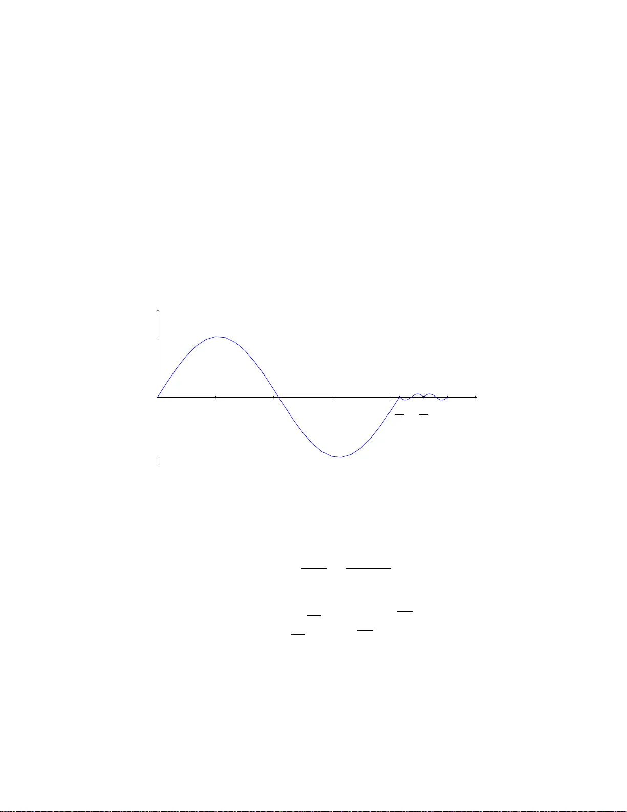
Curv es That Must Be Retraced Xiao y ang Gu ∗ ‡ Jac k H. Lutz †‡ ¶ Elvira Ma y ordomo §¶ k Abstract W e exhibit a p olyno mial time computable plane curve Γ that has finite length, do es no t int ersect itself, and is smo oth e x cept at one endpo int, but has the following proper t y . F or every computable parametriza tion f of Γ a nd every p ositive integer m , there is so me p ositive-length sub c urve of Γ that f retraces at le a st m times. In co n tras t, every computable curve of finite length that do es not intersect itself has a constant-speed (hence non-re tr acing) parametr ization that is computable relative to the halting pr oblem. 1 In tro duction A curve is a m athematical m o del of the path of a particle undergoing con tin uous motio n. Sp ecifi- cally , in a Eu clidean space R n , a curv e is the range Γ of a con tin uous function f : [ a, b ] → R n for some a < b . The f u nction f , called a p ar ametrization of Γ, clearly conta ins more information than the p oin tset Γ, namely , the pr ecise manner in w hic h th e particle “traces” the p oin ts f ( t ) ∈ Γ as t , which is often considered a time p arameter, v a ries from a to b . When the particle’s motion is algorithmicall y go v erned, the p arametrization must b e computable (as a fu n ction on the reals, see b elo w). This paper sho ws that the ge ometry of a curv e Γ ma y force every c omputable paramet rization f of Γ to retrace v arious parts of its path (i.e., “go bac k an d forth along Γ”) man y times, ev en when Γ is an efficien tly compu table, smo oth, finite-length cur v e that do es not inte rsect itself. In fact, our main theorem exhib its a p lane curve Γ ⊆ R 2 with the f ollo wing pr op erties. 1. Γ is simp le , i.e., it do es not in tersec t itself. 2. Γ is r e ctifiable , i.e., it h as finite length. 3. Γ is smo oth exc ept at one endp oint , i.e., Γ has a tangen t at ev ery in terior p oin t and a 1-sided tangen t at o ne endp oin t, and these tangen ts v ary contin uously along Γ . ∗ Department of C omputer Science, Iow a State Universit y , Ames, IA 50011, USA. Email: xiao yang@cs.ia state.edu † Department of Computer S cience, I o wa State Universit y , Ames, IA 50011, U SA. Email: lutz@cs.iastate.edu ‡ Researc h supp orted in part by National Science F oundation Grant 0344 187, 0652569, and 0728806 . § Departamento de Inform´ atica e In genier ´ ıa de S istemas, Universidad de Zaragoza, 50018 Zaragoza, Spain. Email: elvira@unizar.es ¶ Researc h supp orted in part by the Spanish Ministry of Education and S cience (MEC) and th e Europ ean Regional Developmen t F u n d (ERDF) un der pro ject TIN2005-08832-C03-02. k P art of th is author’s researc h w as p erformed during a visit at I o wa State Un ivers ity , su p p orted by Spanish Go vernmen t (S ecretar ´ ıa de Estado de Universidades e Inv estigaci´ o n del Ministerio de Educaci´ on y Ciencia) grant for researc h stays PR2007-0368. 1 4. Γ is p olynomial time c omputa ble in the strong sense that there is a p olynomial time com- putable p osition fun ction ~ s : [0 , 1] → R 2 suc h that the v elo cit y function ~ v = ~ s ′ and the accele ration function ~ a = ~ v ′ are p olynomial time computable; the total distance trav ersed by ~ s is finite; and ~ s paramet rizes Γ , i.e., range( ~ s ) = Γ . 5. Γ must b e r e tr ac e d in the sense that ev ery parametrization f : [ a, b ] → R 2 of Γ that is computable in any amount of time has the follo wing prop ert y . F or ev ery p ositiv e inte ger m , there exist disjoint, closed subin terv a ls I 0 , . . . , I m of [ a, b ] suc h that the cur v e Γ 0 = f ( I 0 ) has p ositiv e lengt h and f ( I i ) = Γ 0 for all 1 ≤ i ≤ m . (Hence f retraces Γ 0 at least m time s.) The terms “c omputable” and “p olynomial time computable” in pr op erties 4 and 5 abov e refer to the “bit-computabilit y” mo del of computation on reals formulate d in the 1950s by Grzegorczyk [9] and Lacom b e [17], extended to f easible compu tabilit y in the 1980s b y Ko and F riedman [13] and Kreitz and W eihr auc h [16], and exp osited in the recen t pap er b y Bra v erman and Co ok [4] a nd the monographs [20, 14, 22, 5]. As will b e shown h ere, condition 4 also implies that the p oin tset Γ is p olynomial time co mputable in the sense of Brattk a and W eihrauc h [2]. (See also [22, 3, 4].) A fund amen tal and usefu l theorem of classical analysis states that ev ery simp le, rectifiable curv e Γ has a normalize d c onstant-sp e e d p ar ametriza tion , whic h is a one-to-one parametrizat ion f : [0 , 1] → R n of Γ with the prop ert y that f ([0 , t ]) has arcle ngth tL for all 0 ≤ t ≤ 1, where L is the le ngth of Γ. (A simple, r ectifiable curv e Γ has exactly t w o suc h p arametrizatio ns, one in ea c h direction, and standard terminology calls either of these the n ormalized constant-speed parametriza- tion f : [0 , 1] → R n of Γ. The constan t-sp eed p arametrizatio n is also called the p ar ametrization by ar clength when it is reformulated as a fu nction f : [0 , L ] → R n that m ov es w ith constant sp eed 1 along Γ.) S ince the constan t-sp eed parametrization do es not retrace any part of the curve, our main theorem implies th at this classical theorem is not en tirely constructive . Ev en when a simple, rectifiable cu r v e has an efficien tly computable parametrization, the constant- sp eed parametrization need not b e computable. In addition to our main theorem, w e pro v e that every sim p le, rectifiable curv e Γ in R n with a computable parametrization has the follo wing t w o p rop erties. I. The length o f Γ is lo w er semicomputable. I I. The constant-speed parametrizat ion of Γ is computable rela tiv e to the length of Γ. These t w o th ings are not hard to p r o v e if the computable parametrizatio n is one-to-one, (in fact, they follo w from results of M ¨ uller and Zhao [19] in this case) but our results hold ev en wh en the computable parametrization retraces p ortions of the curv e many times. T aken together, I and I I ha v e the follo w ing t w o consequences. 1. The curv e Γ of our main theo rem has a finite length that is lo w er semi-c omputable bu t n ot computable. (The existence of p olynomial-time computable curves with this pr op ert y w as first pr o v en by Ko [15].) 2. Ev ery simple, rectifiable curve Γ in R n with a computable parametrization has a constan t- sp eed p arametrizatio n that is ∆ 0 2 -computable, i.e., computable relativ e to the halting pr oblem. Hence, the existe nce of a constan t-speed parametrization, wh ile not en tirely constructiv e, is constructiv e r elativ e to the halting problem. 2 2 Length, Computabilit y , and Complexit y of Curv es In this section we sum marize basic terminology and facts ab out curv es. As w e us e th e terms here, a curv e is the range Γ of a contin uous function f : [ a, b ] → R n for some a < b . The function f is called a parametrization of Γ. Eac h cu r v e clearly has infinitely man y p arametrizations. A cur v e is simple if it h as a parametrization that is one-to-one, i.e., the curve “does not int ersect itself ”. The length of a simp le curv e Γ is d efined as follo ws. Let f : [ a, b ] 1 − 1 → R n b e a one- to-one parametrization of Γ. F or eac h disection ~ t of [ a, b ], i.e., eac h tuple ~ t = ( t 0 , . . . , t m ) with a = t 0 < t 1 < . . . < t m = b , define the f - ~ t -appro ximate length o f Γ to b e L f ~ t (Γ) = m − 1 X i =0 | f ( t i +1 ) − f ( t i ) | . Then the length of Γ is L (Γ) = su p ~ t L f ~ t (Γ) , where the suprem um is tak en o v er all d issections ~ t of [ a, b ]. It is easy to sho w that L (Γ) do es not dep end on the c hoice of the one-to-one p arametrization f , i.e. that the length is an in trinsic prop erty of th e p oin tset Γ. In sections 4 and 5 of this pap er w e u se a more general n otion of length, namely , th e 1- dimensional Hausd orff measure H 1 (Γ), whic h is defined for every set Γ ⊆ R n . W e refer the reader to [7] or the app endix for the definition of H 1 (Γ). It is w ell kn o wn that H 1 (Γ) = L (Γ) holds for ev ery simp le cur v e Γ. A curve Γ is r ectifiable , or has fi nite length if L (Γ) < ∞ . In sections 4 and 5 we use the notation RC for the set of all rectifiable simple cur v es. Definition. Let f : [ a, b ] → R n b e cont inuous. 1. F or m ∈ Z + , f has m - fold r etr acing if there exist disjoint, closed su b in terv als I 0 , . . . , I m of [ a, b ] suc h that the curve Γ 0 = f ( I 0 ) has p ositiv e length and f ( I i ) = Γ 0 for all 1 ≤ i ≤ m . 2. f is no n - r etr acing if f d o es not hav e 1-fold retracing. 3. f h as b ound e d r etr acing if there exists m ∈ Z + suc h that f d o es not hav e m -fold retracing. 4. f has unb ounde d r etr acing if f do es not h av e b ounded retracing, i.e., if f has m -fold retracing for all m ∈ Z + . W e now review the notions of compu tabilit y and complexity of a real-v alued function. An oracle for a real n um b er t is an y fun ction O t : N → Q with the prop ert y th at | O t ( s ) − t | ≤ 2 − s holds f or all s ∈ N . A fu nction f : [ a, b ] → R n is computable if th ere is an oracle T uring mac hine M with the follo wing pr op ert y . F or ev ery t ∈ [ a, b ] and ev ery precision p arameter r ∈ N , if M is giv en r as in put and an y oracle O t for t as its oracle, t hen M outputs a rational p oin t M O t ( r ) ∈ Q n suc h that | M O t ( r ) − f ( t ) | ≤ 2 − r . A function f : [ a, b ] → R n is computable in p olynomial time if there is an oracle mac hine M that do es this in time p olynomial in r + l , wh ere l is the maxim um length of the query resp onses provided b y the oracle. An or acle for a fu nction f : [ a, b ] → R n is an y function O f : ([ a, b ] ∩ Q ) × N → Q n with the prop erty that |O f ( q , r ) − f ( q ) | ≤ 2 − r holds f or all q ∈ [ a, b ] ∩ Q and r ∈ N . A decision pr ob lem 3 A is T uring r e ducible to a fu nction f : [ a, b ] → R n , and we wr ite A ≤ T f , if there is an oracle T u ring machine M su c h that, for ev ery oracle O f for f , M O f decides A . It is easy to see that, if f is computable, then A ≤ T f if an d only if A is deci dable. A cur ve is computable if it has a parametrizatio n f : [ a, b ] → R n , where a, b ∈ Q and f is computable. A curv e is computable in p olynomial time if it h as a p arametrization that is computable in p olynomial time. 3 An Efficien tly Compu table Curv e T hat Must Be Retraced This s ection presen ts our main theorem, whic h is the existence of a smo oth, rectifiable, simple plane cur v e Γ that is parametrizable in p olynomial time b ut not computably parametrizable in an y amoun t of time withou t unb ounded retracing. W e b egin with a precise construction of the curv e Γ , follo w ed by a brief in tuitiv e discuss ion of this construction. The rest of the section is dev oted to proving that Γ has the d esired prop erties. y x − 1 0 1 1 2 3 4 5 25 6 55 12 Figure 3.1: ψ 0 , 5 , 1 Construction 3.1. (1) F or eac h a, b ∈ R with a < b , define the fu nctions ϕ a,b , ξ a,b : [ a, b ] → R by ϕ a,b ( t ) = b − a 4 sin 2 π ( t − a ) b − a and ξ a,b ( t ) =    − ϕ a, a + b 2 ( t ) if a ≤ t ≤ a + b 2 ϕ a + b 2 ,b ( t ) if a + b 2 ≤ t ≤ b. (2) F or eac h a, b ∈ R with a < b and ea c h p ositiv e intege r n , defi n e the fu nction ψ a,b,n : [ a, b ] → R b y ψ a,b,n ( t ) = ( ϕ a,d 0 ( t ) i f a ≤ t ≤ d 0 ξ d i − 1 ,d i ( t ) if d i − 1 ≤ t ≤ d i , 4 where d i = a + 5 b 6 + i b − a 6 n for 0 ≤ i ≤ n . (See Figure 3.1.) (3) Fix a standard en umeration M 1 , M 2 , . . . of (deterministic) T urin g mac hines that ta k e p ositiv e in teger in p uts. F or eac h p ositiv e in teger n , let τ ( n ) denote the n umber of steps executed b y M n on input n . It is w ell kno wn that th e diagonal halting pr oblem K =  n ∈ Z + | τ ( n ) < ∞  is undecidable. (4) Define the horizonta l and v ertical accelerat ion functions a x , a y : [0 , 1] → R as follo ws. F or eac h n ∈ N , let t n = Z n 0 e − x dx = 1 − e − n , noting th at t 0 = 0 and that t n con v erges monotonically to 1 as n → ∞ . Also, for eac h n ∈ Z + , let t − n = t n − 1 + 4 t n 5 , t + n = 6 t n − t n − 1 5 , noting that these are symmetric ab out t n and that t + n ≤ t − n +1 . (i) F or 0 ≤ t ≤ 1, let a x ( t ) = ( − 2 − ( n + τ ( n )) ξ t − n ,t + n ( t ) if t − n ≤ t < t + n 0 if no such n exists , where 2 −∞ = 0. (ii) F or 0 ≤ t < 1, let a y ( t ) = ψ t n − 1 ,t n ,n ( t ) , where n is t he unique p ositiv e intege r suc h that t n − 1 ≤ t < t n . (iii) Let a y (1) = 0. (5) Define the horizon tal and vertic al v elocit y and p osition fun ctions v x , v y , s x , s y : [0 , 1] → R by v x ( t ) = Z t 0 a x ( θ ) dθ , v y ( t ) = Z t 0 a y ( θ ) dθ , s x ( t ) = Z t 0 v x ( θ ) dθ , s y ( t ) = Z t 0 v y ( θ ) dθ . (6) Define the v ect or acce leration, v elocit y , and p osition fu nctions ~ a, ~ v , ~ s : [0 , 1] → R 2 b y ~ a ( t ) = ( a x ( t ) , a y ( t )) , ~ v ( t ) = ( v x ( t ) , v y ( t )) , ~ s ( t ) = ( s x ( t ) , s y ( t )) . 5 (7) Let Γ = range( ~ s ). In tuitiv ely , a p article at rest at time t = a a nd mo ving with acceleration giv en by the function ϕ a,b mo v es forw ard, with v elo cit y increasing to a maxim um at time t = a + b 2 and then d ecreasing bac k to 0 at time t = b . T he vertica l acceleratio n fu nction a y , t ogether with the initial conditions v y (0) = s y (0) = 0 implied b y (5), thus causes a particle to mo ve generally upw ard (i.e., s y ( t 0 ) < s y ( t 1 ) < · · · ), coming to momen tary rests at times t 1 , t 2 , t 3 , . . . . Bet w een t w o consecutiv e suc h stopping times t n − 1 and t n , the particle’s ve rtical acceleratio n is con trolled by the function ψ t n − 1 ,t n ,n . This fun ction causes the particle’s v ertica l motion to do th e f ollo wing b et w een times t n − 1 and t n . (i) F rom time t n − 1 to time t n − 1 +5 t n 6 , mo v e up w ard from elev ation s y ( t n − 1 ) to elev atio n s y ( t n ). (ii) F rom time t n − 1 +5 t n 6 to time t n , mak e n r ound trips to a low er elev atio n s ∈ ( s y ( t n − 1 ) , s y ( t n )). In the mean time, the h orizonta l acceleratio n function a x , together with the initial conditions v x (0) = s x (0) = 0 implied b y (5), ensure that the particle remains on or near the y -axis. The deviations from the y -axis are simply describ ed: The p article mo v es to the r ight from time t n − 1 +4 t n 5 through the completion of the n rou n d trips describ ed in (ii) ab ov e and then mo v es to the y -axis b et w een times t n and 6 t n − t n − 1 5 . The amoun t of lateral motion here is regulated by the co efficien t 2 − ( n + τ ( n )) . I f τ ( n ) = ∞ , then there is no lateral m otion, and the n round trips in (ii) are retracings of the particle’s path. If τ ( n ) < ∞ , then these n roun d trip s are “forw ard” motion along a curvy p art of Γ . In fact, Γ co nta ins p oints of a rbitrarily high curv ature, but th e particle’s motion is kinematically real istic in the sens e that the acceleratio n vec tor ~ a ( t ) is p olynomial time computable, hence cont inuous and b ound ed on the in terv al [0 , 1]. Figure 3.2 illustrates th e path of the particle f rom time t n − 1 to t n +1 with n = 1 and hyp othetical (mo del d ep endent!) v alues τ (1) = 1 a nd τ (2) = 2. y x Figure 3.2: Example of ~ s ( t ) from t 0 to t 2 The rest o f this se ction is d ev oted to pro ving th e follo wing theorem concerning the curve Γ . Theorem 3.2. (main the or em). L et ~ a, ~ v , ~ s , and Γ b e as in Construction 3.1. 1. The functions ~ a, ~ v , and ~ s ar e Li pschitz and c omp utable in p o lynomial time, henc e c ontinuous and b ounde d. 2. The total length, including r etr acings, of the p ar am etrization ~ s of Γ is finite and c omputable in p olynomial time. 6 3. The curve Γ is simple, r e ctifiable, and smo oth exc ept at one endp oint. 4. Every c omputable p ar ametrization f : [ a, b ] → R 2 of Γ has unb ounded r etracing . F or the remainder of this section, w e use the nota tion of Construction 3.1. The follo wing t w o observ a tions facilitate our analysis of the curve Γ . The p ro ofs are routine calculatio ns. Observ at ion 3.3. F or al l n ∈ Z + , if w e write d ( n ) i = t n − 1 + 5 t n 6 + i t n − t n − 1 6 n and e ( n ) i = d ( n ) i + t n − t n − 1 12 n for al l 0 ≤ i < n , then t n − 1 < t − n < d ( n ) 0 < e ( n ) 0 < d ( n ) 1 < e ( n ) 1 < · · · < d ( n ) n − 1 < e ( n ) n − 1 < t n < t + n < t − n +1 . Observ at ion 3.4. F or al l a, b ∈ R with a < b , Z b a Z t a ϕ a,b ( θ ) dθ dt = ( b − a ) 3 8 π . W e now pro ceed with a quantita tiv e analysis of the geometry of Γ . W e b egin with the h orizon tal comp onent of ~ s . Lemma 3.5. 1. F or al l t ∈ [0 , 1] − S n ∈ K ( t − n , t + n ) , v x ( t ) = s x ( t ) = 0 . 2. F or al l n ∈ K and t ∈ ( t − n , t n ) , v x ( t ) > 0 . 3. F or al l n ∈ K and t ∈ ( t n , t + n ) , v x ( t ) < 0 . 4. F or al l n ∈ Z + , s x ( t n ) = ( e − 1) 3 1000 πe 3 n 2 − ( n + τ ( n )) . 5. s x (1) = 0 . Pr o of. Parts 1-3 are routine b y insp ection and induction. F or n ∈ Z + , Obs er v ation 3.4 tells us that s x ( t n ) = ( t n − t − n ) 3 8 π 2 − ( n + τ ( n )) = ( 1 5 ( t n − t n − 1 )) 3 8 π 2 − ( n + τ ( n )) = ( 1 5 (( e − 1) e − n )) 3 8 π 2 − ( n + τ ( n )) = ( e − 1) 3 1000 πe 3 n 2 − ( n + τ ( n )) so 4 holds. This implies that s x ( t n ) → 0 as n → ∞ , w hence 5 follo ws from 1,2, and 3. The follo wing lemma analyzes the v ertical comp onent of ~ s . W e u se the notation of Observ atio n 3.3, with th e ad d itional pr o viso that d ( n ) n = t n . 7 Lemma 3.6. 1. F or al l n ∈ Z + and t ∈ ( t n − 1 , d ( n ) 0 ) , v y ( t ) > 0 . 2. F or al l n ∈ Z + , 0 ≤ i < n , and t ∈ ( d ( n ) i , e ( n ) i ) , v y ( t ) < 0 . 3. F or al l n ∈ Z + , 0 ≤ i < n , and t ∈ ( e ( n ) i , d ( n ) i +1 ) , v y ( t ) > 0 . 4. F or al l n ∈ Z + , 0 ≤ i < n , and t ∈ { e ( n ) i , d ( n ) i , t n } , v y ( t ) = 0 . 5. F or al l n ∈ Z + and 0 ≤ i ≤ n , s y ( d ( n ) i ) = s y ( d ( n ) 0 ) . 6. F or al l n ∈ Z + and 0 ≤ i < n , s y ( e ( n ) i ) = s y ( e ( n ) 0 ) . 7. F or al l n ∈ N , s y ( t n ) = 5 3 ( e − 1) 3 6 3 · 8 π P n i =1 1 e 3 i . 8. F or al l n ∈ Z + , s y ( e ( n ) 0 ) = s y ( t n ) − ( e − 1) 3 12 3 n 3 8 π e 3 n . 9. s y (1) = 5 3 ( e − 1) 3 6 3 · 8 π ( e 3 − 1) . Pr o of. Parts 1-6 are clear by insp ection and induction. By 4. and Observ ation 3.4, s y ( t n ) − s y ( t n − 1 ) = s y ( d ( n ) 0 ) − s y ( t n − 1 ) = [ 5 6 ( t n − t n − 1 )] 3 8 π = [ 5 6 (( e − 1) e − n )] 3 8 π = 5 3 ( e − 1) 3 6 3 · 8 π e 3 n for all n ∈ Z + , so 6 holds by induction. Also b y 4 and Obs erv a tion 3.4, s y ( t n ) − s y ( e ( n ) 0 ) = s y ( d ( n ) 0 ) − s y ( e ( n ) 0 ) = [ 1 12 n ( t n − t n − 1 )] 3 8 π = [ 1 12 n (( e − 1) e − n )] 3 8 π = ( e − 1) 3 12 3 n 3 8 π e 3 n , so 7 holds. Finally , b y 6, s y (1) = 5 3 ( e − 1) 3 6 3 8 π ( e 3 − 1) , i.e., 8 holds. By Lemmas 3.5 and 3.6, we see that ~ s parametrizes a curv e from ~ s (0) = (0 , 0) to ~ s (1) = (0 , 5 3 ( e − 1) 3 6 3 8 π ( e 3 − 1) ). The pro ofs of Lemmas 3.5 and 3.6 are included in the app endix. It is clear from Observ ation 3.3 and Lemmas 3.5 and 3.6 that th e cu r v e Γ do es n ot int ersect itself. W e thus ha v e the f ollo wing. Corollary 3.7. Γ is a simple curve fr om ~ s (0) = (0 , 0) to ~ s (1) = (0 , 5 3 ( e − 1) 3 6 3 8 π ( e 3 − 1) ) . 8 Pr o of. L et ~ s ′ : [0 , 1] → R 2 b e such that ~ s ′ ( t ) = ( ~ s ( t + n ) t − t − n t + n − t − n + ~ s ( t − n ) t + n − t t + n − t − n t ∈ ( t − n , t + n ) , n / ∈ K, ~ s ( t ) otherwise . Note that b y constru ction of ~ s , r etracing happ ens along y -axis b et w een (0 , ~ s ( t − n )) and (0 , ~ s ( t + n )) only when t ∈ ( t − n , t + n ) for n / ∈ K . In ~ s ′ , for all n / ∈ K , ~ s ′ maps ( t − n , t + n ) to the v ertical line segmen t b et w een (0 , ~ s ( t − n )) and (0 , ~ s ( t + n )) linearly . Otherw ise, ~ s ′ ( t ) = ~ s ( t ). Hence, ~ s ′ (0) = (0 , 0), ~ s ′ (1) = (0 , 5 3 ( e − 1) 3 6 3 8 π ( e 3 − 1) ), and ~ s ′ is a one-to-one parametrization of Γ = range( ~ s ), although ~ s ′ is not computable. Th erefore Γ is a sim p le curv e. Lemma 3.8. The functions ~ a, ~ v , and ~ s ar e Lipschitz, henc e c ontinuous, on [0 , 1] . Pr o of. I t is clear by differentiat ion that Lip ( ϕ a,b ) = π 2 for all a, b ∈ R with a < b . It follo ws by insp ection that L ip ( a x ) ≤ π 4 and Lip ( a y ) = π 2 , when ce Lip ( ~ a ) ≤ q Lip ( a x ) 2 + Lip ( a y ) 2 ≤ π √ 5 4 . Th us ~ a is Lipschitz, hence con tin uous (and b ounded), on [0 , 1]. It follo w s immediately t hat ~ v and ~ s are Lipsc hitz, hence cont inuous, on [0 , 1]. Since eve ry Lipschitz parametrization has finite total length [1], and since the length of a curv e cannot exceed the tot al le ngth of any of its parametrizations, w e immediately h av e the follo wing. Corollary 3.9 . The total length, including r etr acings, of the p a r ametr ization ~ s is finite. Henc e the curve Γ is r e ctifiable. Lemma 3.10. The curve Γ is smo oth exc ep t at the endp oint ~ s (1) . Pr o of. W e h a v e seen that Γ ([0 , t − 1 ]) is simply a segment of the y -axis, a nd that the v ec tor velocit y function ~ v is con tin uous o n [0 , 1]. Since the set Z = { t ∈ (0 , 1) | ~ v ( t ) = 0 } has no accum ulation p oin ts in (0 , 1), it therefore suffices to v erify that, for eac h t ∗ ∈ Z , lim t → t ∗− ~ v ( t ) | ~ v ( t ) | = lim t → t ∗ + ~ v ( t ) | ~ v ( t ) | , (3.1) i.e., that t he left and right tangents of Γ coincide at ~ s ( t ∗ ). But this is clear, b ecause Lemmas 3.5 and 3.6 tell us that Z =  t n   n ∈ Z + and τ ( n ) = ∞  , and b oth sid es of (3.1 ) are (0 , 1) a t all t ∗ in this set . Lemma 3.11. The functions ~ a, ~ v , and ~ s ar e c omputable in p olynomial time. The total length including r etr acings, of ~ s is c omputable in p olynomial time. Pr o of. T his follo ws from Observ atio n 3.4, Lemmas 3.5 and 3.6, and the p olynomial time com- putabilit y of f ( n ) = P n i =1 e − 3 i . 9 Definition. A mo dulus of uniform c ontinuity for a fun ction f : [ a, b ] → R n is a function h : N × N suc h that, f or all s , t ∈ [ a, b ] and r ∈ N , | s − t | ≤ 2 − h ( r ) = ⇒ | f ( s ) − f ( t ) | ≤ 2 − r . It is w ell kno wn (e.g., see [14]) that eve ry computable function f : [ a, b ] → R n has a mo du lu s of un iform con tin uit y that is co nt inuous. Lemma 3.12. L et f : [ a, b ] → R 2 b e a p ar ametrization of Γ . If f has b o unde d r etr acing and a c o mputable mo dulus of unifor m c o ntinuity, then K ≤ T f y , wher e f y is the vertic al c omp onent of f . Pr o of. Ass u me the h yp othesis. Then there exist m ∈ Z + and h : N → N su c h that f d o es not ha v e m -fold retracing and h is a computable modu lus of u niform con tin uit y fo r f . Note that h is also a mo dulus of u niform con tin uit y for f y . Let M b e an oracle T u ring mac hine that, giv en an oracl e O g for a f u nction g : [ a, b ] → R , implemen ts the a lgorithm in Figure 3.3. The k ey prop erties of this alg orithm’s choic e of r and ∆ are that th e f ollo wing hold when g = f y . (i) F or eac h time t with f y ( t ) = s y ( t n ), there is a n earby time τ j with j high. Similarly f or f y ( t ) = s y ( e ( n ) 0 ) and j lo w. (ii) F or eac h high j , | f y ( τ j ) − s y ( t n ) | ≤ 3 · 2 − r . S imilarly for eac h lo w j and s y ( e ( n ) 0 ). (iii) No j can b e b oth high a nd lo w. No w let n ∈ Z + . W e sho w that M O f y ( n ) accepts if n ∈ K and rejects if n / ∈ K. This is clear if n ≤ m , so assume th at n > m . If n ∈ K, then Observ ation 3.3, Lemma 3.5, and Lemma 3.6 tell us that M O f y ( n ) accepts. If n / ∈ K, then the fact that f d o es not hav e m -fold retracing tells us that M O f y ( n ) rejects. Pr o of of The or em 3.2. P art 1 follo ws from Lemmas 3.8 and 3.11. Pa rt 2 follo ws from Lemma 3.11. P art 3 follo ws from Corollaries 3.7 and 3.9 and L emm a 3.10. P art 4 follo ws from Lemma 3.12 , the f act th at ev ery computable fu nction g : [ a, b ] → R 2 has a computable mod ulus of uniform con tin uit y , and th e f act that A is decidable wherev er A ≤ T g and g is computable. 4 Lo w e r Semicomputabilit y of L ength In this section we pro v e that ev ery computable curve Γ has a lo wer semicomputable length. Our pro of is somewhat in v olv ed, b ecause o ur result h olds ev en if ev ery co mpu table p arametrization of Γ is r etracing. Construction 4.1. Let f : [0 , 1] → R n b e a computable function. Giv en an oracle T u ring mac hine M th at computes f and a computable mo d ulus m : N → N of the u niform con tin uit y of f , the ( M , m )-cautious p olygonal appro ximator of range( f ) is the f unction π M ,m : N → { pol y g onal paths } computed by the follo wing algorithm. input r ∈ N ; S := {} ; // S ma y be a multi-set 10 input n ∈ Z + ; if n ≤ m then use a fi n ite lo okup table to accept if n ∈ K a nd reject if n / ∈ K else b egin r := the least p ositiv e in teger s uc h that 2 3 − r < s y ( t n ) − s y ( e ( n ) 0 ); ∆:=2 − h ( r ) ; for 0 ≤ j ≤ ( b − a ) / ∆ do b egin τ j := a + ∆ j ; call j high if |O g ( τ j , r ) − s y ( t n ) | < 2 1 − r call j lo w if |O g ( τ j , r ) − s y ( e ( n ) 0 | < 2 1 − r end ; if there is a sequ ence 0 < j 0 < j 1 < · · · < j m in which j i is high for all e ve n i and lo w for a ll o dd i then accept else reject end . Figure 3.3: Algorithm for M O g ( n ) in th e pro of of Lemma 3.12. for i :=0 t o 2 m ( r ) do a i := i 2 − m ( r ) ; use M to compute x i with | x i − f ( a i ) | ≤ 2 − ( r + m ( r )+1) ; add x i to S; output a longest path inside a minimum spanning tree of S . Definition. Let ( X , d ) b e a metric space. Let Γ ⊆ X and ǫ > 0. Let Γ( ǫ ) =  p ∈ X     inf p ′ ∈ Γ d ( p, p ′ ) ≤ ǫ  b e the Mi nkowski sausage of Γ with radius ǫ . Let d H : P ( X ) × P ( X ) → R b e su c h that for a ll Γ 1 , Γ 2 ∈ P ( X ) d H (Γ 1 , Γ 2 ) = inf { ǫ | Γ 1 ⊆ Γ 2 ( ǫ ) and Γ 2 ⊆ Γ 1 ( ǫ ) } . Note that d H is the Hausdorff distanc e fun ction. Let K ( X ) b e the set of nonempty compact su bsets of X . Th en ( K ( X ) , d H ) is a metric s p ace [6]. Theorem 4.2. (F rink [8], Mic hael [18]). L et ( X, d ) b e a c omp act metric sp ac e. Then ( K ( X ) , d H ) is a c omp act metric sp ac e. Definition. Let RC b e the set of a ll simp le rectifiable cur v es in R n . 11 Theorem 4.3. ([21] p age 55). L et Γ ∈ RC . L et { Γ n } n ∈ N ⊆ RC b e a se quenc e of r e c tifiable c urves such that lim n →∞ d H (Γ n , Γ) = 0 . Then H 1 (Γ) ≤ lim inf n →∞ H 1 (Γ n ) . This theorem has th e f ollo wing consequence. Theorem 4.4. L et Γ ∈ RC . F or al l ǫ > 0 , ther e exists δ > 0 such that for al l Γ ′ ∈ RC , if d H (Γ , Γ ′ ) < δ , then H 1 (Γ ′ ) > H 1 (Γ) − ǫ . In the follo wing, we pro v e a few tec hnical lemmas that lead to Lemma 4.9, whic h p la ys an imp ortant r ole in pr o vin g T heorem 4.10. Lemma 4.5. L et Γ ∈ RC . L et p 0 , p 1 , ∈ Γ b e its two endp oints. L et Γ ′ ( Γ such that p 0 , p 1 ∈ Γ ′ . Then Γ ′ / ∈ RC . Pr o of. If Γ ′ is not closed, then w e a re done. Assume that Γ ′ is closed. Let γ b e a parametrization of Γ su c h that γ (0) = p 0 and γ (1) = p 1 . Since Γ ′ 6 = Γ an d p 0 , p 1 ∈ Γ ′ , γ − 1 (Γ ′ ) ⊆ I 0 ∪ I 1 , where I 0 ⊆ [0 , 1] and I 1 ⊆ [0 , 1] are closed and disjoin t. It is easy to see that γ ( I 0 ) and γ ( I 1 ) are closed and disj oint. And th us, for any con tinuous function γ ′ : [0 , 1] → R n , γ ′− 1 ( γ ( I 0 )) and γ ′− 1 ( γ ( I 1 )) are closed and disjoint. T herefore, f or any con tinuous fun ction γ ′ : [0 , 1] → R n , γ − 1 (Γ ′ ) 6 = [0 , 1], i.e., Γ ′ / ∈ RC . Lemma 4.6. L et Γ ∈ RC . L et Γ ′ ⊆ Γ b e a c onne cte d c omp act set. Then Γ ′ ∈ RC . Pr o of. Let γ b e the p arametrization of Γ. Let a = inf { γ − 1 (Γ ′ ) } and let b = sup { γ − 1 (Γ ′ ) } . Let γ ′ : [0 , 1] → R n b e such that for all t ∈ [0 , 1] γ ′ ( t ) = γ ( a + t ( b − a )) . Then γ ′ defines a curve and we sho w that γ ′ ([0 , 1]) = Γ ′ . It is clear th at Γ ′ ⊆ γ ′ ([0 , 1]). Since Γ ′ is compact, we kno w that γ ′ (0) , γ ′ (1) ∈ Γ ′ . Supp ose for s ome t ′ ∈ (0 , 1), γ ′ ( t ′ ) / ∈ Γ ′ . Since Γ ′ is compact, there exists ǫ > 0 s uc h that γ ′ ([ t ′ − ǫ, t ′ + ǫ ]) ∩ Γ ′ = ∅ . Then Γ ′ ⊆ γ ′ ([0 , t ′ − ǫ )) ∪ γ ′ (( t ′ + ǫ, 1]). Since γ ′ is one-one, d H ( γ ′ ([0 , t ′ − ǫ )) , γ ′ (( t ′ + ǫ, 1])) > 0 . Hence, d H (Γ ′ ∩ γ ′ ([0 , t ′ − ǫ )) , Γ ′ ∩ γ ′ (( t ′ + ǫ, 1])) > 0 . Th us, Γ ′ cannot b e connected. Therefore, if Γ ′ is connected, th en Γ ′ = γ ′ ([0 , 1]) and hence Γ ′ ∈ RC . Lemma 4.7. L et Γ 0 , Γ 1 , . . . b e a c onver ge nt se quenc e of c omp act sets in c omp act metric sp ac e ( X, d ) that is eventual ly c onne cte d. L et Γ = lim n →∞ Γ n . Then Γ is c onne c te d. Pr o of. W e p ro v e t he contrapositiv e. Assume th at Γ is not connected. Th en there exists op en sets A, B ⊆ X such that A ∩ B = ∅ , Γ ∩ A 6 = ∅ , Γ ∩ B 6 = ∅ , and Γ ⊆ A ∪ B . Then (Γ ∩ A ) ∩ (Γ ∩ B ) = ∅ , thus d H (Γ ∩ A, Γ ∩ B ) > 0. Let δ = d H (Γ ∩ A, Γ ∩ B ) . 12 Since lim n →∞ Γ n = Γ, let n 0 b e suc h that for all n ≥ n 0 , d H (Γ n , Γ) ≤ δ 3 . It is clear th at (Γ ∩ A )( δ 3 ) ∩ Γ n 6 = ∅ , (Γ ∩ B )( δ 3 ) ∩ Γ n 6 = ∅ , and Γ n ⊆ (Γ ∩ A )( δ 3 ) ∪ (Γ ∩ B )( δ 3 ) . By the defin ition of δ , d H ((Γ ∩ A )( δ 3 ) , (Γ ∩ B )( δ 3 )) ≥ δ 3 . Th us Γ n is not connected for all n ≥ n 0 . Lemma 4.8. L et Γ ∈ RC and let f : [0 , 1] → Γ b e a p ar ametrization of Γ . L et L (Γ , ǫ ) = inf  H 1 (Γ ′ )   Γ ′ ∈ RC and Γ ′ ⊆ Γ( ǫ ) and f (0) , f (1) ∈ Γ ′  . Then lim ǫ → 0 + L (Γ , ǫ ) = H 1 (Γ) . Pr o of. It i s cle ar th at lim ǫ → 0 + L (Γ , ǫ ) ≤ H 1 (Γ). It su ffices to sh o w that lim ǫ → 0 + L (Γ , ǫ ) ≥ H 1 (Γ). Let δ > 0. F or eac h i ∈ N , let S i =  Γ ′ ∈ RC   Γ ′ ⊆ Γ( 1 i ) and γ (0) , γ (1) ∈ Γ ′  , where γ is a parametrization of Γ. Note that if i 2 < i 1 , then S i 1 ⊆ S i 2 . Let Γ 0 , Γ 1 , . . . b e an arbitrary sequence suc h that for all i ∈ N , Γ i ∈ S k i , and k 0 , k 1 , · · · ∈ N is a strictly incr easing sequence. Since for all i ∈ N , Γ i is compact and co nnected, b y Theorem 4.2 and Lemma 4.7, there is at least one cluster p oint and every cluster p oin t is a connected compact set. Let Γ ′ b e a cluster p oint. It is clear th at Γ ′ ⊆ Γ. T hen b y Lemma 4.6, Γ ′ ∈ RC . It is also clear that γ (0) , γ (1) ∈ Γ ′ b y d efinition of S i . T h us by Lemma 4.5, Γ ′ = Γ. By Theorem 4.3, lim inf n →∞ H 1 (Γ n ) ≥ H 1 (Γ ′ ) = H 1 (Γ). Then by T heorem 4.4, this implies that for all sufficient ly la rge i ∈ N , ( ∀ Γ ′′ ∈ S i ) H 1 (Γ ′′ ) ≥ H 1 (Γ) − δ . Therefore, for a ll s u fficien tly large i ∈ N , L (Γ , 1 i ) ≥ H 1 (Γ) − δ . Since δ > 0 is a rbitrary , lim ǫ → 0 + L (Γ , ǫ ) ≥ H 1 (Γ) . Lemma 4.9. L et Γ ∈ RC and let f : [0 , 1] → Γ b e a p ar ametrization of Γ . L et L (Γ , ǫ, p 1 , p 2 ) = inf  H 1 (Γ ′ )   Γ ′ ∈ RC and Γ ′ ⊆ Γ( ǫ ) and p 1 , p 2 ∈ Γ ′  . Then lim ǫ → 0 + sup p 1 ,p 2 ∈ Γ( ǫ ) L (Γ , ǫ, p 1 , p 2 ) = H 1 (Γ) . 13 Pr o of. F or ev ery p ∈ Γ( ǫ ), there exists a p oin t p ′ ∈ Γ such that k p, p ′ k ≤ ǫ and line segmen t [ p, p ′ ] ⊆ Γ( ǫ ). Thus it is clear that f or all p 1 , p 2 ∈ Γ( ǫ ), L (Γ , ǫ, p 1 , p 2 ) ≤ 2 ǫ + H 1 (Γ). Th erefore, lim ǫ → 0 + sup p 1 ,p 2 ∈ Γ( ǫ ) L (Γ , ǫ, p 1 , p 2 ) ≤ H 1 (Γ) . F or the other direction, obs erv e that lim ǫ → 0 + sup p 1 ,p 2 ∈ Γ( ǫ ) L (Γ , ǫ, p 1 , p 2 ) ≥ lim ǫ → 0 + L (Γ , ǫ ) . Applying Lemma 4.8 co mpletes the pro of. Theorem 4.10. L et Γ ∈ RC such th at Γ = γ ([0 , 1] ) , wher e γ is a c ontinuous function. (Note that γ may not b e one-one.) L et S ( a ) = { γ ( a i ) | a i ∈ a } for al l disse ction a . L et { a n } n ∈ N b e a se quenc e of disse ctions of Γ such that lim n →∞ mesh( a n ) = 0 . Then lim n →∞ H 1 ( LM S T ( a n )) = H 1 (Γ) , wher e LM S T ( a ) is the longest p ath inside the Minimum Eu clide an Sp anning T r e e of S ( a ) . Pr o of. F or a ll n ∈ N , let ǫ n = 2 d H (Γ , S ( a n )) . Note that s in ce γ is uniformly con tinuous and lim n →∞ mesh( a n ) = 0, lim n →∞ ǫ n = 0. Let w = 2 ǫ n . Claim. L et T b e a Eu clide an Sp anning T r e e of S ( a ) . If T has an e dge that is not inside Γ( w ) , then T is not a minimum sp anning tr e e. Pr o of of Claim. Let E b e an edge of T suc h that E * Γ( w ). T h en H 1 ( E ) > 2 w . Removing E from T will br eak T in to t w o subtrees T 1 , T 2 . By the defin ition of ǫ n and the con tinuit y of γ , there exists s 1 , s 2 ∈ S ( a ) with k s 1 − s 2 k ≤ ǫ n suc h that s 1 ∈ T 1 and s 2 ∈ T 2 . It is clear that T 1 ∪ T 2 ∪ { ( s 1 , s 2 ) } is also a Euclidean Span n ing T ree of S ( a ) and H 1 ( T 1 ∪ T 2 ∪ { ( s 1 , s 2 ) } ) < H 1 ( T ), i.e ., T is not minimum. Let T b e a Minimum Eu clidean S panning T r ee of S ( a ). L et L b e the longest p ath inside T . Then L ⊆ T ⊆ Γ( w ). Note that H 1 ( L ) ≤ H 1 (Γ). Let p 0 , p 1 b e the tw o endp oin ts of Γ. Since L is the longest p ath ins ide T and p 0 , p 1 are eac h within ǫ n distance to some p oin t in S ( a n ), L (Γ , w , p 0 , p 1 ) ≤ 2 ǫ n + H 1 ( L ) . By Lemma 4.9, lim w → 0 + L (Γ , w , p 0 , p 1 ) = H 1 (Γ) . Then lim n →∞ H 1 ( LM S T ( a n )) = H 1 (Γ) . 14 This r esu lt implies that wh en the samp lin g dens ity is high, th e n umb er of lea v es in the minimum spanning tree is asymptotic ally smalle r than the total num b er of no d es. W e no w h a ve the mac hinery to pro v e the main result of this s ection. Theorem 4.11. L et γ : [0 , 1] → R n b e c omputable such that Γ = γ ([0 , 1]) ∈ RC . Then H 1 (Γ) is lower semic omputable. Pr o of. Let the function f , M , and m in Cons truction 4.1 b e γ , a computation of γ , and its computable mo d ulus resp ectiv ely . F or eac h input r ∈ N , π M ,m ( r ) is the longest path L r in M S T ( S r ), where S r is the set of p oin ts sampled by π M ,m ( r ). Let l r = H 1 ( L r ) − 2 − r . Note that l r is computable fr om r ∈ N . W e sho w that f or all r ∈ N , l r ≤ H 1 (Γ) and lim r →∞ l r = H 1 (Γ). Let ˜ f b e a one-one parametrization of Γ. Let π : { 0 , . . . , 2 m ( r ) } → { 0 , . . . , 2 m ( r ) } b e a p erm uta- tion of { 0 , . . . , 2 m ( r ) } such th at for all i, j ∈ { 0 , . . . , 2 m ( r ) } , i < j = ⇒ ˜ f − 1 ( f ( a π ( i ) )) < ˜ f − 1 ( f ( a π ( j ) )) . Let ˆ Γ r b e the p olygonal curve connecting the p oints f ( a π (0) ) , f ( a π (1) ) , . . . , f ( a π (2 m ( r ) ) ) in order . Then ˆ Γ r is a polygonal app ro x im ation of Γ and H 1 ( ˆ Γ r ) ≤ H 1 (Γ). Let ¯ Γ r b e the p olygonal curve connecting the p oin ts in S r in the ord er of x π (0) , x π (1) , . . . , x π (2 m ( r ) ) . Due to the ap p ro ximation in duced by the co mputation in C onstruction 4.1, H 1 ( ¯ Γ r ) ≤ H 1 ( ˆ Γ r ) + 2 − r . Then it is cle ar t hat H 1 ( L r ) = H 1 ( LM S T ( S r )) ≤ H 1 ( ¯ Γ r ) ≤ H 1 ( ˆ Γ r ) + 2 − r . Th us l r ≤ H 1 ( ˆ Γ r ) . Let ˆ S r = { f ( a 0 ) , f ( a 1 ) , . . . , f ( a 2 m ( r ) ) } . Note that ˆ S r ma y b e a multi-set. By Theorem 4.1 0, lim r →∞ LM S T ( ˆ S r ) = H 1 (Γ) . Let ǫ r = 2 d H (Γ , S r ) . By Contruction 4.1, lim r →∞ ǫ r = 0 . Let w r = 2 ǫ r . Let T r b e a Minimum Euclidean Spann in g T r ee of S r . Let L r b e the longest p ath inside T r . By the Claim in Theorem 4.10 , L ⊆ T ⊆ Γ( w r ). By an essentia lly iden tical argumen t as the one in t he proof o f Th eorem 4.10, lim r →∞ l r = lim r →∞ H 1 ( LM S T ( S r )) = H 1 (Γ) , whic h completes the p ro of. 15 5 ∆ 0 2 -Computabilit y of the Constan t-Sp eed P arametrization In this section w e prov e that ev ery computable curve Γ has a constan t sp eed parametrization that is ∆ 0 2 -computable. Theorem 5.1. L e t Γ = γ ∗ ([0 , 1]) ∈ RC . ( γ ∗ may not b e one-one.) L et l = H 1 (Γ) and O l b e an or acle such that for al l n ∈ N , | O l ( n ) − l | ≤ 2 − n . L et f b e a c omputation of γ ∗ with mo dulus m . L et γ b e the c onstant sp e e d p ar ametrization of Γ . Then γ i s c omputable with or acle O l . Pr o of. O n input k as the precision parameter for compu tation of the curve and a rational num b er x ∈ [0 , 1] ∩ Q , we output a point f k ( x ) ∈ R n suc h that | f k ( x ) − γ ( x ) | ≤ 2 − k . Without loss of generalit y , assume that H 1 (Γ) > 1000 · 2 − k . Let δ = 2 − (4+ k ) . Run f as in Construction 4.1 w ith increasingly larger pr ecision parameter r > − log δ unt il H 1 ( LM S T ( a )) > H 1 (Γ) − δ 2 and the shortest distance b et w een the t w o endp oin ts of LM S T ( a ) inside the p olygonal sau s age around LM S T ( a ) with width 2 d = 2 · 2 − r is at least H 1 (Γ) − δ 2 . This can b e ac hieved by usin g Euclidean shortest p ath algorithms [1 2, 11]. Let d k ≤ 2 − (4+ k ) b e the largest d su c h th at the ab ov e conditions are satisfied, w hic h is assur ed b y Theorem 4.11 and Lemma 4.9. Let S b e the p olygonal sausage around LM S T ( a ) with width 2 d k . F or p 1 , p 2 ∈ S , let d S ( p 1 , p 2 ) = the s hortest distance b et w een p 1 and p 2 inside S . Note th at S is connected. Let f k b e the constan t sp eed p arametrization of LM S T ( a ) and γ b e the constan t sp eed parametrization of Γ. Without loss of generalit y , assu m e that k γ (0) − f k (0) k < k γ (1) − f k (0) k and k γ (1) − f k (1) k < k γ (0) − f k (1) k , since we can hardco de approxima te lo cations of γ (0) an d γ (1) suc h that when d k is suffi cien tly small, we can decide w eh ther a sampled p oint is closer to γ (0) or γ (1). As w e n o w pro v e lim k →∞ { f k (0) , f k (1) } = { γ (0) , γ (1) } . Note th at for eac h s ∈ S suc h that s / ∈ LM S T ( a ), there exists p ∈ LM S T ( a ) ∩ S suc h that the shortest p ath from s to p in M S T ( a ) has length less than δ 2 , i.e., d M S T ( a ) ( s, p ) < δ 2 , since H 1 ( LM S T ( a )) > H 1 (Γ) − δ 2 and H 1 ( M S T ( a )) ≤ H 1 (Γ). Let δ 0 = d S ( γ (0) , f k (0)). Let s 0 b e the closest p oint to γ (0) in S ∩ LM S T ( a ). Th en d S ( γ (0) , s 0 ) ≤ δ 2 + d k . Then d LM S T ( a ) ( s 0 , f k (0)) ≥ δ 0 − δ 2 − d k . Since s 0 ∈ S ∩ LM S T ( a ) and we assume H 1 (Γ) > 1000 · 2 − k , d S ( s 0 , γ (1)) ≤ H 1 ( LM S T ( a )) − δ 0 + δ 2 + d k + δ 2 + d k = H 1 ( LM S T ( a )) − δ 0 + δ + 2 d k . Then d S ( γ (0) , γ (1)) ≤ H 1 ( LM S T ( a )) − δ 0 + δ + 2 d k + δ 2 + d k < H 1 ( LM S T ( a )) − δ 0 + 3 δ 2 + 3 d k . And hence d S ( γ (0) , γ (1)) ≤ H 1 (Γ) − δ 0 + 2 δ + 3 d k . (5.1) 16 By th e c hoice of d k , we ha v e that d S ( f k (0) , f k (1)) ≥ H 1 (Γ) − δ 2 . Now, note that for an y tw o p oint s p 1 , p 2 ∈ Γ, d S ( p 1 , p 2 ) ≤ H 1 (Γ) + d S ( γ (0) , γ (1)) 2 , since we can put them in h alf of a loop. Therefore d S ( f k (0) , f k (1)) ≤ H 1 (Γ) + d S ( γ (0) , γ (1)) 2 . Th us d S ( γ (0) , γ (1)) ≥ H 1 (Γ) − δ . (5.2) By (5.1) and (5.2), w e h a ve δ 0 ≤ 3 δ + 3 d k ≤ 6 δ < 2 − k , (5.3) i.e., k f k (0) − γ (0) k ≤ d S ( f k (0) , γ (0)) ≤ 6 δ < 2 − k . (5.4) Similarly , k f k (1) − γ (1) k ≤ d S ( f k (1) , γ (1)) ≤ 6 δ < 2 − k . (5.5) No w w e pro ceed to show that for all t ∈ (0 , 1), k f k ( t ) − γ ( t ) k < 10 δ with f (0) b eing at most 6 δ from γ (0) insid e S and f (1) b eing at most 6 δ f r om γ (1) inside S . Let ∆ k = k f k ( t ) − γ ( t ) k . Let s f ∈ S ∩ LM S T ( a ) b e such that | f − 1 k ( s f ) − t | is min imized. Then d LM S T ( a ) ( f k ( t ) , s f ) ≤ d k , since ev ery edge in M S T ( a ) is at most d k long. Let s ′ γ ∈ S ∩ Γ b e suc h that | γ − 1 ( s ′ γ ) − t | is minimized. Then d Γ ( γ ( t ) , s ′ γ ) ≤ d k , since we sample S u s ing d k as the densit y parameter. Let s γ ∈ S ∩ LM S T ( a ) such that d M S T ( a ) ( s γ , s ′ γ ) is m inimized. Then d M S T ( a ) ( s γ , s ′ γ ) ≤ δ 2 , since H 1 ( M S T ( a )) ≥ H 1 (Γ) − δ 2 . Then k f k ( t ) − s γ k ≥ ∆ k − ( δ 2 + d k ) = ∆ k − δ 2 − d k . Note that d LM S T ( a ) ( s f , s γ ) ≥ k s f − s γ k ≥ ∆ k − δ 2 − 2 d k . Without loss of generalit y , assu me that distance f rom s γ to f k (0) along LM S T ( a ) is ∆ k − δ 2 − d k more than the distance from f k ( t ) to f k (0). Otherwise, we sim p ly lo ok from the γ (1) and f k (1) side instead. The path traced b y γ fr om γ (0) to γ ( t ) has length t · H 1 (Γ). The shortest distance b et w een γ ( t ) to s γ inside Γ ∪ M S T ( a ) is at m ost d k + δ 2 . The path traced b y f k from s γ to f k (1) has length d LM S T ( a ) ( s γ , f k (1)) ≤ H 1 ( LM S T ( a )) − [ t ( H 1 (Γ) − δ 2 ) − d k + ∆ k − δ 2 − d k ] . The shortest distance f rom γ (1) to f k (1) inside S is at most 6 δ . Then the d istance from γ (0) to γ (1) inside S is at most t · H 1 (Γ) + d k + δ 2 + H 1 ( LM S T ( a )) − [ t ( H 1 (Γ) − δ 2 ) − d k + ∆ k − δ 2 − d k ] + 6 δ ≤ H 1 ( LM S T ( a )) + 3 d k + 8 δ − ∆ k ≤ H 1 (Γ) + 11 δ − ∆ k . By (5.2) , w e h a ve ∆ k ≤ 12 δ < 2 − k . 17 Corollary 5.2. L et Γ b e a curve with the pr op erty describ e d in pr op erty 5 of The or em 3.2. Then the length of Γ – H 1 (Γ) is no t c omputable. Pr o of. W e p ro v e the cont rap ositiv e. Let Γ b e a curv e with a computable parametrization with a computable length H 1 (Γ). Then by Theorem 5.1, we can use the T u r ing mac hine th at computes H 1 (Γ) as the oracle in the statemen t of T heorem 5.1 and obtain a T uring mac hine that computes the constan t sp eed parametrization of Γ. Therefore, Γ do es not hav e th e prop erty describ ed in item 5 of Theorem 3.2 . 6 Conclusion As w e ha v e noted, Ko [15] has pro ve n the existence of computable curv es with finite, b ut u ncom- putable lengths, and the c urve Γ of our main th eorem is one suc h curv e. In the recen t pap er [10], w e ha v e giv en a precise c haracterizatio n of those p oints in R n that lie on compu table curv es of finite length. With these things in mind, w e p ose the follo wing. Question. Is there a p oin t x ∈ R n suc h that x lies on a computable curv e of finite length b ut not on any computable curve of computable length? Ac knowledgmen t. W e thank anonymo us r eferees for their v aluable co mments. References [1] T. M. Ap ostol. Intr o duction to Analytic Numb er The ory . Undergradu ate T exts in Mathematics. Springer-V erlag, 1976. [2] V. Brattk a and K. W eihrauch. Computability on subsets of Euclidean space I: C losed and compact sub sets. The or etic al Computer Scienc e , 219:65–9 3, 1999. [3] M. Bra ve rman. On the complexit y o f real fun ctions. In F orty-Sixth Annual IEEE Symp osium on F oundations of Computer Scienc e , 2005. [4] M. B ra ve rman and S. Cook. Computing ov er the reals: F oundations for scien tific computing. Notic es of the A MS , 53(3 ):318–32 9, 2006. [5] M. B ra ve rman and M. Y amp olsky . Computability of Julia Sets . Springer, 2008. [6] G. A. E d gar. Me asur e, top olo gy, and fr actal ge ometry . Springer-V erlag, 1990. [7] K. F alconer. F r actal Ge ometry: Mathematic al F oundations and Applic ations . Wile y , second edition, 2003. [8] O. F rin k, Jr. T op ology in lattices. T r ansactions of the Am eric an Mathematic al So ciety , 51(3): 569–582 , 1942. [9] A. Grze gorczyk. Computable functionals. F undamenta Mathematic ae , 42:168–202 , 1955. [10] X. Gu, J . H. Lutz, and E. Ma yordomo. Poin ts on computable curv es. In Pr o c e e dings of the F orty-Seventh Ann ual IEEE Symp osium on F oundations of Computer Scienc e , pages 469–474. IEEE Compu ter S o ciet y Press, 2006. 18 [11] J. Hershb erger and S. S uri. An optimal algorithm for euclidean sh ortest paths in the plane. SIAM Journal on Computing , 28(6):2215– 2256, 1999. [12] S. Kap o or and S . N. Mahesh w ari. Efficient algorithms for euclidean shortest path and visi- bilit y problems with p olygonal obstacles. In Pr o c e e dings of the fourth annual symp osium on c omputationa l ge ometry , pages 172–182, New Y ork, NY, USA, 1988. ACM Press. [13] K. Ko and H. F riedman. Computational complexit y of real functions. The or etic al Computer Scienc e , 20:323–3 52, 1982. [14] K.-I. K o. Complexity The ory of R e al F unctions . Birkh¨ auser , B oston, 19 91. [15] K.-I. Ko. A p olynomial-time computable curve wh ose interior has a nonrecursive measure. The or etic al Computer Scienc e , 145:241 –270, 1995. [16] C. Kr eitz and K . W eihrauch. C omplexit y theory on real num b ers and fu nctions. In The or etic al Computer Scienc e , v olume 145 of L e ctur e Notes in Com puter Scienc e . S pringer, 1982. [17] D. Laco mbe. Extension de la n otion de fonctio n recursive aux fonctions d’une ou plusiers v ariables reelles, and other notes. Comptes R endus , 240: 2478-24 80; 241:1 3-14, 151-153, 1250- 1252, 1955. [18] E. Mic h ael. T op ologies on spaces of su bsets. T r ansactions of the Americ an Mathematic al So cie ty , 71(1):15 2–182, 1951. [19] N. T. M¨ uller and X. Zh ao. Jord an a reas and grids. In Pr o c e e dings of the Fifth International Confer enc e on Com putability and Complexity in A nalysis , pag es 191–206, 200 8. [20] M. B. P our-El and J. I. R ichards. Comp utability in Analysis and P hysics . Springer-V erlag, 1989. [21] C. T ricot. Curves a nd F r actal Dimension . Springer-V erlag, 1995. [22] K. W eihrauc h. Computable An alysis. An Intr o duction . S pringer-V erlag, 2000. 19