Simultaneous support recovery in high dimensions: Benefits and perils of block $ell_1/ell_infty$-regularization

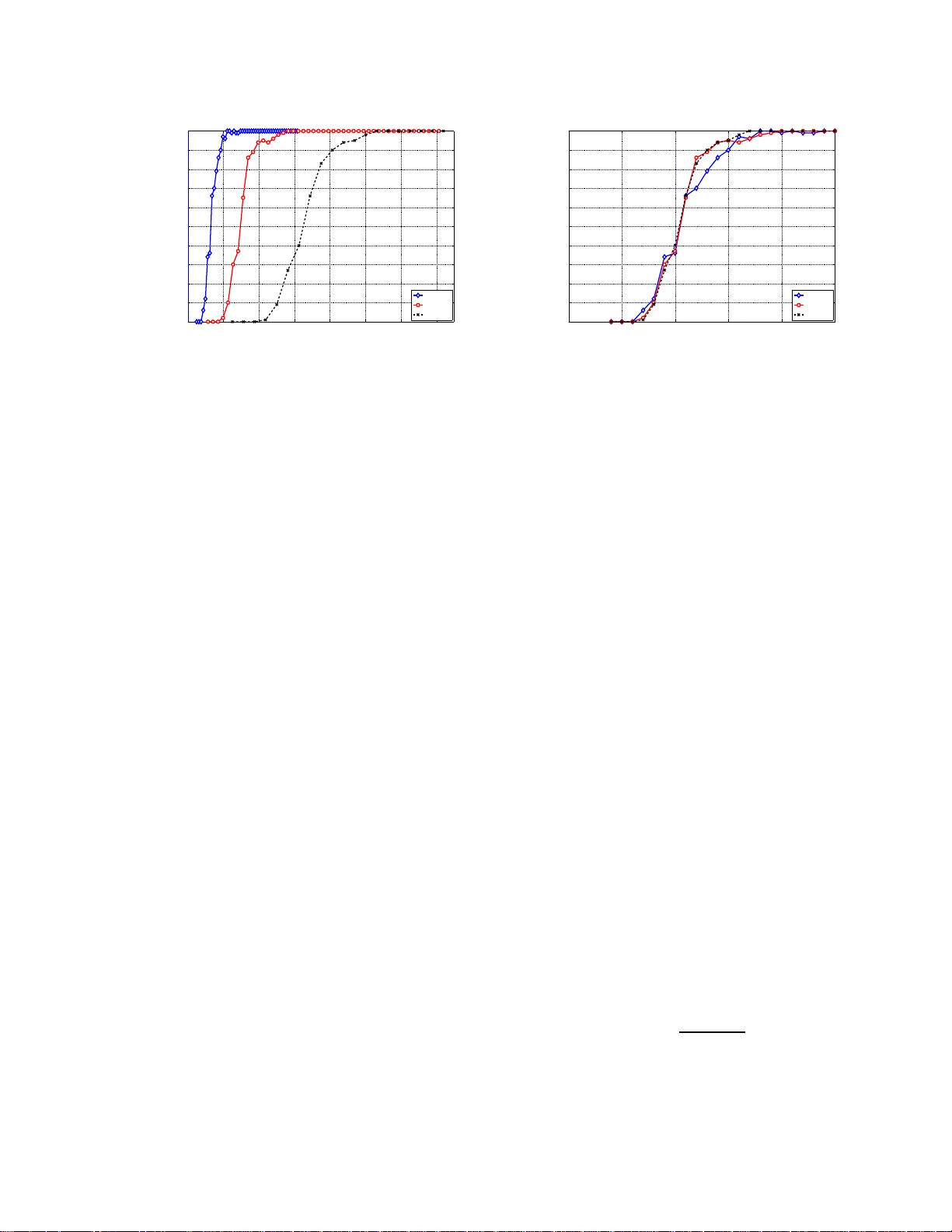
Sim ultaneous supp ort reco v ery in high dimensio n s: Beneﬁt s and p erils of bl o c k ℓ 1 /ℓ ∞ -regularizati on Sahand Negah ban ⋆ Martin J. W ain wright † ,⋆ Departmen t of Sta tistics † , and Departmen t of Electrical En gineering and Computer S ciences ⋆ UC Berk eley , Berk eley , CA 94720 Ma y 5, 2009 T ec hnical Rep ort, Departmen t of Statistics, UC Berk eley Abstract Given a collectio n of r ≥ 2 linea r r egressio n problems in p dimensions, supp ose that the regres s ion coeﬃcients share partially common suppo r ts. This set-up sugg ests the use of ℓ 1 /ℓ ∞ -regular ized regres s ion for joint e s timation o f the p × r matr ix of regr es- sion co eﬃcients. W e analyze the high- dimensional scaling o f ℓ 1 /ℓ ∞ -regular ized quadratic progra mming, co nsidering bo th co ns istency rates in ℓ ∞ -norm, and also how the mini- mal sample size n r e quired for p erfo rming v aria ble selection grows as a function of the mo del dimension, sparsity , and ov erlap b etw een the supp orts. W e b e g in b y esta blish- ing b ounds o n the ℓ ∞ -error as well suﬃcient conditio ns for exac t v ariable s election for ﬁxed de s ign matrice s , a s well as designs drawn r andomly from g eneral Gauss ia n matri- ces. Our seco nd set of results applies to r = 2 linear reg ression problems with standar d Gaussian designs whose supp orts ov erla p in a fractio n α ∈ [0 , 1] of their entries: fo r this problem class, we pro ve that the ℓ 1 /ℓ ∞ -regular ized metho d undergo es a phase tra nsition— that is, a sharp ch a nge from failure to s uccess—characterized b y the resca led sample size θ 1 , ∞ ( n, p, s, α ) = n/ { (4 − 3 α ) s log ( p − (2 − α ) s ) } . More precisely , given seq ue nc e s o f problems speciﬁed by ( n, p, s, α ), for any δ > 0, the proba bility of succe ssfully re cov ering bo th supp orts converges to 1 if θ 1 , ∞ ( n, p, s, α ) > 1 + δ , and conv erg es to 0 for pro blem sequences for which θ 1 , ∞ ( n, p, s, α ) < 1 − δ . An implicatio n of this threshold is tha t use of ℓ 1 /ℓ ∞ -regular ization yields improved statistica l eﬃcie nc y if the overlap parameter is large enoug h ( α > 2 / 3), but ha s worse statistical eﬃciency tha n a naive L asso-ba s ed approach for mo der ate to small ov er la p ( α < 2 / 3). Empirical s im ulatio ns illustra te the close agreement b etw een these theoretical predictions , a nd the actual behavior in practice. These results indicate that so me caution needs to be exercised in the applica tion of ℓ 1 /ℓ ∞ blo ck regula rization: if the data does not matc h its s tructure closely enough, it can impair statistical perfor mance relative to computationally less expensive schemes. 1 1 In tro duc tion The area of h igh-d imensional statistical inference is concerned with the b eha vior of mo d els and algorithms in which the dimen s ion p is comparable to, or p ossibly eve n larger than the sample size n . In the absence of additional structur e, it is well-kno wn th at many standard pro cedures—among them linear regression and principal comp onent analysis—are not consis- ten t u nless the ratio p/n con v erges to zero. Since this scaling precludes having p comparable 1 This w ork was presented in part at t h e NIPS 2008 conference in V ancouver, Canada, Decem b er 2008. Supp orted in part by NSF grants DMS- 0528488, DMS-0605165, and CCF-0545862. 1 to or larger than n , an activ e line of researc h is based on imp osing str u ctural conditions on the data (e.g., sparsit y , manifold constraints, or grap h ical mo del structur e), and studying the high-dimensional consistency (or inconsistency) of v arious t yp es of estimators. This p ap er deals with high-dimensional scali n g in the context of s olving m ultiple regression problems, wh ere the regression v ectors are assumed to ha v e sh ared sp arse stru cture. More sp eciﬁcally , su pp ose that w e are give n a collection of r diﬀeren t linear regression mo d els in p dimensions, with regression v ectors β i ∈ R p , for i = 1 , . . . , r . W e let S ( β i ) = { j | β i j 6 = 0 } denote the su pp ort set of β i . In many applications—among them spars e approxi mation, graphical mo del selection, and image r econstru ction—it is natural to imp ose a sp arsit y con- strain t, corresp onding to restricting the cardin alit y | S ( β i ) | of eac h sup p ort set. Moreo v er, one m igh t exp ect some amount of o ve rlap b et wee n the sets S ( β i ) and S ( β j ) f or indices i 6 = j since they corresp ond to the sets of activ e regression co eﬃcien ts in eac h p roblem. Let us consider some examples to illustrate: • Consid er the problem of image denoising or compr ession, sa y using a wa velet transform or some other t yp e of m ultiresolution basis [17]. It is wel l kno wn that natural images tend to hav e sparse representat ions in such bases [27]. Moreo ver, similar images—sa y the same scene tak en fr om multiple cameras—w ould b e exp ected to share a s imilar subset of activ e f eatures in the reconstruction. Consequen tly , one m igh t exp ect that using a blo c k-regularizer that enforces s uc h join t sparsit y could lead to impro ve d image denoising or compression. • Consid er the problem of id en tifying the s tr ucture of a Mark o v net wo rk or graph ical mo del [10] based on a collection of samples (e.g. , such as observ ations of a so cial net- w ork). F or net w orks with a single parameter p er edge (e.g., Gaussian mod els [19], Isin g mo dels [25]), a line of r ecen t work has shown that ℓ 1 -based metho ds can b e successful in reco v ering the net work structure. Ho wev er, many graphical m o dels h a v e m ultiple parameters p er edge (e.g., for d iscr ete mo dels with non-b in ary state spaces), and it is natural that the su bset of parameters asso ciated with a giv en edge are zero (or n on- zero) in a group ed manner. T hus, any metho d f or reco ve rin g the graph structure should imp ose a blo c k-structured regularization that groups toget h er the subset of parameters asso ciated with a single edge. • Finally , consider a standard problem in genetic analysis: giv en a set of gene expression arra ys, where eac h arra y corresp ond s to a diﬀerent p atien t but the same u nderlying tissue t yp e (e.g., tum or), the goal is to disco v er the su bset of f eatures relev an t for tumorous gro wths . T his problem can b e expressed as a join t regression pr oblem, again with a shared sparsit y constrain t coupling together the diﬀerent p atien ts. In this con text, the recen t w ork of Liu et al. [14] shows that imp osing additional stru ctural constrain ts can b e b eneﬁcial (e.g., th ey are able to greatly reduce the num b er of expr essed genes while mainta inin g the same prediction p erf ormance). Giv en these stru ctur al conditions of s hared sparsity in these and other app lications, it is reasonable to consider how this common s tructure can b e exploited so as to increase the statistica l eﬃciency of estimation pro cedur es. There is n o w a su bstan tial and relativ ely mature b o d y of w ork on ℓ 1 -regularizatio n for estimation of sparse mo d els, dating back to the in tro duction of the Lasso and basis p ursuit [28, 5]. With con tribu tions from v arious r esearchers (e.g., [7, 19, 29, 37, 3]), there is n o w a fairly complete th eory of the b ehavi or of the L asso for high-dimens ional spars e estimation. A more 2 recen t line of work (e.g., [31, 35, 22, 30, 36]), motiv ated by app lications in wh ic h blo c k or hierarc hical stru cture arises, has p rop osed the use of b lo c k ℓ a,b norms for v arious a, b ∈ [1 , ∞ ]. Of particular relev ance to this pap er is the blo c k ℓ 1 /ℓ ∞ norm, pr op osed in itially by T ur lac h et al. [31] and T ropp et al. [30]. Th is form of b lo ck regularization is a sp ecia l case of th e more general family of comp osite or hierarchica l p enaltie s, as stud ied b y Z hao et al. [36]. V arious authors ha ve empirically demonstrated that blo c k regularizati on schemes can yield b etter p erf orm ance for diﬀerent data s ets [36, 22, 14]. Some recen t w ork by Bac h [1] has pro vided consistency results for ℓ 1 /ℓ 2 blo c k-regularization sc hemes under classical scaling, meaning th at n → + ∞ with p ﬁxed. Meier et al. [18] has established h igh-dimensional consistency for the predictiv e r isk of ℓ 1 /ℓ 2 blo c k-regularized logisti c regression. The pap ers [15, 21, 24] ha v e pr o vided high-dimensional consistency results for ℓ 1 /ℓ q blo c k r egularizatio n for supp ort reco very us ing ﬁxed design matrices, but the r ates do n ot pr o vide sharp diﬀerences b et ween the case q = 1 and q > 1. T o date, there has a r elativ ely limited amount of theoretical w ork c h aracterizing if and when the use of blo c k regularization sc hemes actually leads to gains in statisti cal eﬃciency . As w e elab orate b elo w, th is question is signiﬁcant due to th e greater computational cost in v olve d in solving blo ck-reg ularized con v ex programs. In the case of ℓ 1 /ℓ 2 regularization, concurrent w ork b y Ob ozinski et al [23] (inv olving a subset of the cur ren t authors) h as s h o wn that that the ℓ 1 /ℓ 2 metho d can yield statistical gains up to a factor of r , the num b er of separate r e- gression pr ob lems; m ore recen t concurren t work [9, 16] has provided related high-dimensional consistency r esults for ℓ 1 /ℓ 2 regularization, emphasizing the gains when th e num b er of tasks r is muc h larger than log p . This pap er considers this issue in the con text of v ariable s election using blo c k ℓ 1 /ℓ ∞ regularization. Our main contribution is to obtain some precise—and arguably surpr ising— insigh ts in to the b eneﬁts and d angers of usin g blo c k ℓ 1 /ℓ ∞ regularization, as compared to simpler ℓ 1 -regularizatio n (separate Lasso f or eac h regression problem). W e b egin b y p ro viding a general set of suﬃ cien t conditions for consistent sup p ort reco very for b oth ﬁxed design matrices, and r andom Gaussian d esign matrices. In addition to these basic consistency results, w e then seek to c haracterize rates, for the particular case of standard Gaussian designs, in a manner pr ecise en ou gh to addr ess the follo wing questions: (a) First, und er what stru ctural assump tions on the d ata do es the use of ℓ 1 /ℓ ∞ blo c k- regularization pr o vide a quant iﬁab le reduction in the scaling of the sample size n , as a function of the prob lem dimension p and other structural parameters, required for consistency? (b) Second, are there an y settings in wh ich ℓ 1 /ℓ ∞ blo c k-regularization can b e harmfu l rel- ativ e to computationally less exp ensive p r o cedures? Answ ers to these questions yield us eful insigh t in to th e tr ade oﬀ b etwe en c omputatio nal and sta- tistic al eﬃcie nc y in high-dimensional inference. Indeed, the con v ex p r ograms that arise from using blo ck-regula r ization t ypically require a greater computational cost to solve . Accord- ingly , it is imp ortant to und erstand u nder what conditions this increased computational cost guaran tees that fewe r samples are r equired for ac hieving a ﬁxed level of statistical accuracy . The analysis of this pap er giv es conditions on the d esigns and regression matrix B for wh ic h ℓ 1 /ℓ ∞ yields impro v ements (question (a)), and also sho ws that if there is s u ﬃcien t mismatc h b et ween the regression matrix B and the ℓ 1 /ℓ ∞ norm, then use of this r egularizer actually impairs statistical eﬃciency r elativ e to a n aiv e ℓ 1 -approac h. As a r epresen tativ e instance of our theory , consider the sp ecial case of standard Gaussian design matrices and t w o r egression 3 problems ( r = 2), with the su pp orts S ( β 1 ) and S ( β 2 ) eac h of size s and o ve r lapp ing in a fraction α ∈ [0 , 1] of their ent ries. F or th is problem, we pr o v e that blo ck ℓ 1 /ℓ ∞ regularization undergo es a phase transition—meaning a sharp thr eshold b etwe en suc c ess and r e c overy —that is sp eciﬁed by the rescaled sample size θ 1 , ∞ ( n, p, s, α ) : = n (4 − 3 α ) s log( p − (2 − α ) s ) . (1) In w ord s, for any δ > 0 and for scalings of the qu ad r uple ( n, p, s, α ) su c h that θ 1 , ∞ ≥ 1 + δ , the p robabilit y of successfully reco v ering b oth S ( β 1 ) and S ( β 2 ) con v erges to one, whereas for scalings suc h that θ 1 , ∞ ≤ 1 − δ , the probabilit y of success conv erges to zero. Figure 1 illustrates h o w the theoretical threshold (1) agrees w ith the b eha vior observed in practice. This ﬁ gu r e plots the probab ility of s u ccessful reco v ery u s ing the blo c k ℓ 1 /ℓ ∞ approac h ve rs u s the rescaled sample size n/ { 2 s log [ p − (2 − α ) s } ; the r esults sho wn here are for r = 2 regression parameters. The plots sho w t welv e curve s, corresp ond ing to three diﬀeren t prob lem sizes p ∈ { 128 , 256 , 512 } and four diﬀerent v alues of th e ov erlap parameter α ∈ { 0 . 1 , 0 . 3 , 0 . 7 , 1 } . First, let us fo cus on the set of curv es lab eled with α = 1, corresp onding to case of complete ov erlap b et wee n the regression vec tors. Notice ho w the curves for all three problem s izes p , wh en plotted v ersus the r escaled sample s ize, lin e up w ith one another; this “stac king eﬀect” sh o ws that the rescaled s amp le size captures the phase transition b ehavio r. Similarly , for other c hoices of the o verlap, the sets of three curv es (o ver problem size p ) exhibit the same stac king b eha vior. Secondly , note that the results are consisten t with th e theoretical prediction (1): the stac ks of curves sh ift to the righ t as the o v erlap parameter α decreases 0 1 2 3 4 5 0 0.2 0.4 0.6 0.8 1 Control parameter θ Prob. success ℓ 1 , ∞ relaxation for s = 0.1*p and α = 1 , 0 . 7 , 0 . 4 , 0 . 1 p = 128 p = 256 p = 512 α = 1 α = 0 . 7 α = 0 . 4 α = 0 . 1 α = 1 α = 0 . 7 α = 0 . 4 α = 0 . 1 α = 1 α = 0 . 7 α = 0 . 4 α = 0 . 1 Figure 1. Pr obability of success in r ecov ering the joint signed supp orts plo tted against the rescaled sample siz e θ Las : = n/ [2 s lo g( p − (2 − α ) s ))] for linear sparsity s = 0 . 1 p . Ea ch stack of gr aphs corresp onds to a ﬁxed ov erla p α , as lab eled on the ﬁg ure. The three curves within each s tack corresp ond to problem sizes p ∈ { 128 , 2 56 , 51 2 } ; no te how they all a lign with each other and exhibit step-like behavior, consistent with Theorem 3. The vertical lines cor resp ond to the thresholds θ ∗ 1 , ∞ ( α ) predicted by Theorem 3; note the close agreement betw een theor y and simulation. from 1 to w ards 0, sho wing that problems with less o ve r lap require a larger rescaled sample size. More interesting is the sh arpness of agreemen t in quantitative terms: the vertica l lines 4 in the cen ter of eac h s tac k sho w th e p oin t at wh ic h our theory (1) predicts that the metho d should transition fr om failure to su ccess. By comparison to pr evious theory on th e b ehavio r of the Lasso (ordinary ℓ 1 -regularized quadratic programming), the scaling (1) h as tw o in teresting implications. F or the s -sparse re- gression p roblem with standard Gaussian designs, the Lasso has b een shown [33] to transition from success to failure as a f unction of the rescaled sample size θ Las ( n, p, s ) : = n 2 s log ( p − s ) . (2) In particular, under the conditions imp osed here, solving tw o separate Lasso problems, one for eac h regression problem, wo u ld reco ver b oth supp orts for p roblem sequen ces ( n, p , s ) suc h that θ Las > 1. T hus, one consequence of ou r analysis is to c haracterize the r elative statistic al eﬃciency of ℓ 1 /ℓ ∞ regularization v ersu s ordinary ℓ 1 -regularizatio n , as describ ed by the ratio R : = θ 1 , ∞ θ Las . Our theory predicts that (disregarding some o (1) factors) the relativ e eﬃciency scales as R ( α ) ∼ 4 − 3 α 2 , whic h (as w e sho w later) sho ws excellen t agreement with empirical b eh avior in simulatio n . Our characte rization of R ( α ) conﬁrm s that if the regression matrix B is we ll- aligned with the b lo c k ℓ 1 /ℓ ∞ regularizer—more sp eciﬁcally for o verlaps α ∈ [ 2 3 , 1]—then block- regularization increases statistical eﬃciency . On the other hand, our analysis also con veys a c autiona ry message : if th e ov erlap is to o sm all—more pr ecisely , if α < 2 / 3—then blo c k ℓ 1 , ∞ is actually relativ e to th e naiv e Lasso-based app roac h. T his fact illustrates that some care is required in th e application of b lo c k regularization sc hemes. In terms of pr o of tec hn iques, the analysis of this pap er is considerably more delicate than the an alogous argument s r equired to sho w su p p ort consistency f or the L asso [19, 33, 37]. The ma jor diﬀerence—and one that p resen ts su bstan tial tec hnical c hallenges—is that the sub-diﬀerentia l 2 of the blo c k ℓ 1 /ℓ ∞ is a m uch m ore subtle ob ject than the sub diﬀeren tial of the ord in ary ℓ 1 -norm. In particular, the ℓ 1 -norm has an ordinary d er iv ativ e wh enev er the co eﬃcien t vect or is non-zero. In con trast, ev en for non-zero ro ws of the r egression m atrix, the b lo ck ℓ 1 /ℓ ∞ norm may b e n on -d iﬀeren tiable, and these non-d iﬀerentiable p oints pla y a k ey role in our analysis. (See Section 4.1 for more detail on the su b -diﬀeren tial of this blo ck norm.) As we sho w, it is the F rob en ius norm of the sub-diﬀerentia l on the regression matrix supp ort that con trols high-dimensional scaling. F or th e ordinary ℓ 1 -norm, this F rob en iu s norm is alw a ys equal to s , wh ereas for matrices with r = 2 columns and α fr action o ve r lap, this F rob enius norm can b e as small as (4 − 3 α ) s 2 . As our analysis revea ls, it is precisely the diﬀering structur es of these su b-diﬀeren tials that leads to d iﬀeren t high-d im en sional scaling for ℓ 1 v ersus ℓ 1 , ∞ regularization. The remainder of this pap er is organized as follo ws. In Section 2, w e pr o vide a pr ecise description of the pr oblem. Section 3 is devot ed to the statemen t of our main resu lts, some discussion of their consequences, and illustration by comparison to emp irical simulatio ns . In Section 4 , we pr ovide an outline of the pr o of, with the tec h n ical details of many intermediate lemmas deferred to the app end ices. Notational con v entions: F or the con venience of the reader, w e su mmarize here some notation to b e used throughout the pap er. W e reserv e the ind ex i ∈ { 1 , . . . , r } as a sup erscrip t 2 As we d escribe in m ore detail in Section 4.1 , the sub-diﬀerential is th e app ropriate generalization of gradient to conv ex fun ctions th at are allow ed to hav e “corners”, like the ℓ 1 and ℓ 1 /ℓ ∞ norms; the standard b o oks [26, 8] conta in more bac k ground on sub-diﬀerentials and their p rop erties. 5 in ind exing th e diﬀerent regression problems, or equ iv alen tly the columns of the matrix B ∈ R p × r . Giv en a design matrix X ∈ R n × p and a subset S ⊆ { 1 , . . . , p } , w e use X S to denote the n × | S | sub-matrix obtained by extracting those columns in dexed b y S . F or a p air of matrices A ∈ R m × ℓ and B ∈ R m × n , we use the notation  A, B  : = A T B for the resu lting ℓ × n matrix. W e use the follo wing standard asymptotic notation: for fun ctions f , g , the n otation f ( n ) = O ( g ( n )) means that there exists a ﬁxed constan t 0 < C < + ∞ such that f ( n ) ≤ C g ( n ); the notation f ( n ) = Ω( g ( n )) means that f ( n ) ≥ C g ( n ), and f ( n ) = Θ( g ( n )) means th at f ( n ) = O ( g ( n )) and f ( n ) = Ω ( g ( n )). 2 Problem set-up W e b egin by setting u p the problem to b e s tu died in this pap er, including multiv ariate re- gression and f amily of blo c k-regularized programs for estimating sparse vec tors. 2.1 Multiv ariate regression and blo c k regularization sc hemes In this pap er, w e consider the follo wing form of m ultiv ariate regression. F or eac h i = 1 , . . . , r , let β i ∈ R p b e a regression vecto r, and consider the r -v ariate linear regression pr oblem y i = X i β i + w i , i = 1 , 2 , . . . , r. (3) Here eac h X i ∈ R n × p is a d esign matrix, p ossibly diﬀeren t for eac h v ector β i , and w i ∈ R n is a noise v ector. W e assume that the noise vect ors w i and w j are ind ep endent for diﬀerent regression problems i 6 = j . In this pap er, w e assume that eac h w i has a multiv ariate Gaussian N (0 , σ 2 I n × n ) distr ib ution. Ho w eve r , we note that qu alitativ ely similar results will hold for an y noise distribution with sub-Gaussian tails (see the b o ok [4] f or more bac kground on su b- Gaussian v ariates). F or compactness in notation, w e frequently use B to denote the p × r matrix with β i ∈ R p as the i th column. Give n a p arameter q ∈ [1 , ∞ ], we deﬁne the ℓ 1 /ℓ q blo c k-norm as follo ws: k B k ℓ 1 /ℓ q : = p X k =1 k ( β 1 k , β 2 k , . . . , β r k ) k q , (4) corresp ondin g to applying the ℓ q norm to eac h ro w of B , and the ℓ 1 -norm across all of these blo cks. W e n ote that all of these blo c k norms are sp ecial cases of the C AP family of p enalties [36]. This family of b lo ck-regularize rs (4) suggests a natur al family of M -estimators for esti- mating B , based on solving the blo c k- ℓ 1 /ℓ q -regularized quadratic p rogram b B ∈ arg min B ∈ R p × r  1 2 n r X i =1 k y i − X i β i k 2 2 + λ n k B k ℓ 1 /ℓ q  , (5) where λ n > 0 is a user-deﬁn ed regularization parameter. Note that the data term is separable across the diﬀeren t regression problems i = 1 , . . . , r , d u e to our assum ption of in dep enden ce on the noise vect ors. Any coupling b et w een the diﬀeren t regression p roblems is indu ced by the blo ck-norm regularizat ion. In the sp ecial case of univ ariate r egression ( r = 1), the parameter q p la ys no role, and the b lo c k-regularized scheme (6 ) red u ces to the Lasso [28, 5]. If q = 1 and r ≥ 2, the 6 blo c k-regularization fun ction (like th e data term) is separable across th e diﬀerent regression problems i = 1 , . . . , r , and so the scheme (6) redu ces to solving r s ep arate Lasso p roblems. F or r ≥ 2 an d q = 2, the program (6) is frequently referr ed to as the group Lasso [35, 22]. Another imp ortant case [31, 30] and the fo cus of this pap er is the setting q = ∞ and r ≥ 2, whic h we refer to as blo c k ℓ 1 /ℓ ∞ regularization. The motiv ati on for usin g blo c k ℓ 1 /ℓ ∞ regularization is to encourage shar e d sp arsity among the columns of the regression matrix B . Geometrically , lik e the ℓ 1 norm that u nderlies the ordinary Lasso, th e ℓ 1 /ℓ ∞ blo c k norm has a p olyhedr al un it ball. Ho w eve r, the blo c k norm captures p oten tial inte r actions b etw een the columns β i in the matrix B . Intuitiv ely , taking the maximum encourages the element s ( β 1 k , β 2 k . . . , β r k ) in any giv en ro w k = 1 , . . . , p to b e zero simultaneously , or to b e n on-zero simultaneously . Indeed, if β i k 6 = 0 for at least one i ∈ { 1 , . . . , r } , then there is n o additional p enalt y to ha ve β j k 6 = 0 as w ell, as long as | β j k | ≤ | β i k | . 2.2 Estimation in ℓ ∞ norm and supp or t recov ery F or a giv en λ n > 0, s upp ose that w e solv e th e blo c k ℓ 1 /ℓ ∞ program, thereby obtaining an estimate b B ∈ arg min B ∈ R p × r  1 2 n r X i =1 k y i − X i β i k 2 2 + λ n k B k ℓ 1 /ℓ ∞  , (6) W e n ote that u nder high-dimen sional scaling ( p ≫ n ), this con v ex program (6) is n ot n eces- sarily strictly conv ex, since the quadratic term is rank deﬁcient and th e blo ck ℓ 1 /ℓ ∞ norm is p olyhedral, whic h implies that the program is not strictly conv ex. Ho w ever, a consequence of our analysis is th at under appr op r iate conditions, the optimal solution b B is in fact unique. In this p ap er, we study the accuracy of the estimate b B , as a f u nction of the sample size n , regression d im en sions p and r , and the sp ars it y index s = max i =1 ,...,r | S ( β i ) | . Th ere are v arious metrics with wh ic h to assess th e “clo seness” of the estimate b B to the truth B , including predictiv e risk, v arious t yp es of norm -based b ounds on the d iﬀeren ce b B − B , and v ariable selection consistency . In this pap er, we prov e results b ound ing the ℓ ∞ /ℓ ∞ diﬀerence k b B − B k ℓ ∞ /ℓ ∞ : = max k =1 ,...,p max i =1 ,...,r | b B i k − B i k | . In addition, w e prov e results on sup p ort reco v ery criteria. Recall that f or eac h vec tor β i ∈ R p , w e u se S ( β i ) = { k | β i k 6 = 0 } to d enote its supp ort set. The problem of r ow supp ort r e c overy corresp onds to reco vering th e set U : = r [ i =1 S ( β i ) , (7) corresp ondin g to the subset U ⊆ { 1 , . . . , p } of indices that are activ e in at least one regression problem. Note that the cardinalit y of | U | is up p er b ounded by r s , but can b e substantia lly smaller (as small as s ) if there is o ve rlap among the diﬀeren t supp orts. As d iscussed at more length in App endix A, giv en an estimate of the ro w supp ort of B , it is p ossible to either u se additional structure of th e solution b B or p erform some additional computation to reco v er individual signe d supp or ts of the columns of B . T o b e pr ecise, deﬁne the sign fu nction sign( t ) =      +1 if t > 0 0 if t = 0 − 1 if t < 0. (8) 7 Then the r eco v ery of individu al signed supp orts means estimating the signed vecto rs with en tries sign( β i k ), for eac h i = 1 , 2 , . . . , r an d for all k = 1 , 2 , . . . , p . In terestingly , w hen using blo c k ℓ 1 /ℓ ∞ regularization, there are m ultiple wa ys in whic h the supp ort (or signed supp ort) can b e estimated, d ep ending on whether we use primal or dual information from an optimal solution. The dual r e c overy metho d inv olv es the f ollo wing steps. First, solv e the b lo ck-regularize d program (6 ), thereby obtaining an prim al solution b B ∈ R p × r . F or eac h ro w k = 1 , . . . , p , compute the set M k : = arg max i =1 ,...,r | b β i k | . Estimate the supp ort u nion via b U = S i =1 ,...,r S ( b β i ), and estimate the signed supp ort ve ctors [ S dua ( b β i k )] = ( sign( b β i k ) if i ∈ M k 0 otherwise. (9) As our deve lopment will clarify , this pro cedu r e (9 ) corresp onds to estimating the signed supp ort on the basis of a dual optimal s olution asso ciated with the optimal pr imal solution. W e discuss the primal-based reco very m etho d and its diﬀerences with the dual-based metho d at more length in App endix A. 3 Main results and their consequences In this section, we pro vide precise statemen ts of th e main results of this pap er. O ur ﬁ rst main result (Theorem 1) provides suﬃcien t conditions for deterministic d esign matrices X 1 , . . . , X r , whereas our second main resu lt (Theorem 2) p ro vides suﬃcient conditions for design matrices dra wn r andomly from sub-Gaussian ensembles. Both of these results allo w for an arbitrary n umb er r of regression pr oblems, and th e random design case allo ws for r an d om Gaussian designs X k with i.i.d. rows and co v ariance matrix Σ k ∈ R p × p , k = 1 , . . . , r . Not surpr isin gly , these resu lts show that the high-dimensional s caling of blo c k ℓ 1 /ℓ ∞ is qualitatively similar to that of ordinary ℓ 1 -regularizatio n : for instance, in th e case of random Gaussian designs and b ounded r , our suﬃcien t conditions ens ure that n = Ω( s log p ) samp les are su ﬃcien t to reco v er the union of supp orts correctly with high p r obabilit y , whic h matc hes k n o wn results on th e Lasso [33], as well as kno wn information-theoretic r esults on the problem of su p p ort reco v ery [32]. As d iscussed in the in tro du ction, we are also intereste d in the more reﬁned qu estion: can w e pr o vide necessary and suﬃcient conditions that are sh arp enough to r ev eal quantita- tive diﬀer enc es b et w een ordinary ℓ 1 -regularizatio n and blo ck regularization? Addressing this question requires analysis that is suﬃcien tly pr ecise to con trol the constan ts in fr ont of the rescaled sample size n/s log( p − s ) that con trols the p erformance of b oth ℓ 1 and blo c k ℓ 1 /ℓ ∞ metho ds. Accordingly , in order to provide precise answers to this qu estion, our ﬁnal tw o results concern the sp ecial case of r = 2 regression problems, b oth with supp orts of size s that o v erlap in a fraction α of their en tries, and w ith design matrices dra wn r an d omly from th e standard Gaussian ensem b le. In this setting, our ﬁnal r esu lt (Theorem 3) sho ws that b lo ck ℓ 1 /ℓ ∞ regularization undergo es a ph ase transition—that is, a rapid c hange from failure to success—sp eciﬁed b y the rescaled s amp le size θ 1 , ∞ ( n, p, s, α ) previously d eﬁned (1). W e then discuss some consequen ces of these r esults, and illustrate their s harpness with some sim u lation results. 8 3.1 Suﬃcien t conditions for general deterministic and random designs In addition to the sample size n , pr oblem d imensions p and r , sparsity index s and o ver- lap parameter α , our results inv olv e certain quantitie s asso ciated with the d esign matrices X i . T o b egin, in the deterministic case, we assu me that th e columns of eac h design m atrix X i , i = 1 , . . . , r are normalized 3 so that k X i k k 2 2 ≤ 2 n for all k = 1 , 2 , . . . p . (10) More signiﬁcantl y , we require that the follo wing inc oher enc e c ond ition on the d esign m atrix b e satisﬁed: γ (Σ ) : = 1 − max ℓ =1 ,..., | U c | r X i =1 k  X i ℓ , X i U ( h X i U , X i U i ) − 1  k 1 > 0 . (11) F or the case of the ordinary Lasso, conditions of this t yp e are known [19, 37, 33] to b e b oth necessary and s u ﬃcien t for successful supp ort reco very . 4 In addition, the statement of our results in vo lve certain quan tities associated with the | U | × | U | m atrices 1 n h X i U , X i U i ; in particular, we deﬁne a lo wer b ound on th e minim um eigen v alue C min ( X ) ≤ min i =1 ,...,r λ min  1 n h X i U , X i U i  , (12) as we ll as an up p er b ound maximum ℓ ∞ , ∞ -op erator norm of th e in ve rs es D max ( X ) ≥ max i =1 ,...,r | | |  1 n h X i U , X i U i  − 1 | | | ∞ . (13) Remem b erin g that our analysis applies to to sequences { X n,p } of design matrices, in the simplest scenario, b oth of the b ounding quant ities C min and D max do not scale with ( n, p, s ). T o k eep notation compact, w e write C min and D max in the analysis to f ollo w. W e also deﬁn e the supp ort minimum value B min = min k ∈ U max i =1 ,...,r | β i k | , (14) corresp ondin g to the minim um v alue of the ℓ ∞ norm of any row k ∈ U . Theorem 1 (S u ﬃcien t conditions for deterministic designs) . Consider the observation mo del (3) with design matric es X i satisfying the c olumn b ound (10) and inc oher enc e c ondition (11) . Supp ose that we solve the blo ck-r e gularize d ℓ 1 /ℓ ∞ c onvex pr o gr am (6) with r e gu larization p a- r am eter λ 2 n ≥ 4 ξ σ 2 γ 2 r 2 + r l og( p ) n for some ξ > 1 . Then with pr ob ability gr e ater than φ 1 ( ξ , p, s ) : = 1 − 2 exp( − ( ξ − 1)[ r + log p ]) − 2 exp( − ( ξ 2 − 1) log( r s )) , (15) we ar e guar ante e d that (a) The blo ck-r e gularize d pr o gr am has a uniqu e solution b B such that S r i =1 S ( b β i ) ⊆ U . 3 The choice of the factor 2 in t his b ound is for later t echnical con venience. 4 Some w ork [20] h as shown that multi-stag e method s can allow some relaxation of th is incoherence cond ition; how ev er, as our main interest is in u nderstanding t he sample complexity of ordinary ℓ 1 versus ℓ 1 /ℓ ∞ relaxations, w e do not pursue such extensions here. 9 (b) Mor e over, the solution satisﬁes the elementwise ℓ ∞ -b ound k b B − B k ℓ ∞ /ℓ ∞ ≤ ξ s 4 σ 2 C min log | U | n + D max λ n | {z } . (16) b 1 ( ξ , λ n , n, s ) Conse quently, as long as B min ≥ b 1 ( ξ , λ n , n, s ) , then S r i =1 S ( b β i ) = U , so that the solu- tion b B c orr e ctly sp e c iﬁes the union of supp orts U . W e now state an analogous result for rand om design matrices; in particular, consider the observ ation mo del (3 ) with design matrices X i c hosen with i.i.d. rows from cov ariance matrices Σ i . In analogy to deﬁn itions (12) and (13) in the deterministic case, w e deﬁne the lo w er b ound C min (Σ ) ≤ min i =1 ,...,r λ min  Σ i U U  , (17) as we ll as an analogous upp er b oun d on ℓ ∞ -op erator norm of th e inv erses D max (Σ ) ≥ max i =1 ,...,r | | | (Σ i U U ) − 1 | | | ∞ ≤ D max . (18) Note that u n lik e the case of deterministic designs, these qu an tities are not functions of th e design matrix X , which is no w a random v ariable. Finally , our r esults inv olv e an analogous incoherence parameter of the co v ariance m atrices Σ = { Σ i , i = 1 , . . . , r } , d eﬁned as γ (Σ ) : = 1 − max k =1 ,..., | U c | r X i =1   Σ i k U (Σ i U U ) − 1   1 > 0 . (19) With th is notation, the follo win g result provides an analog of Th eorem 1 for random design matrices: Theorem 2 (Suﬃcien t conditions for random Gaussian designs) . Supp ose that we ar e given n i.i.d. observations fr om the mo del (3) with n > 8 κ r C min γ 2 s  r + log p  (20) for some κ > 1 . If we solve the c onvex pr o gr am (6 ) with r e gulariza tion p ar am eter satisfying λ n ≥ 4 ξ σ 2 γ 2  r 2 + r l og( p ) n ] f or some ξ > 1 , then with pr ob ability gr e ater than φ 2 ( κ, ξ , n, p, s ) : = 1 − 2 exp  − 2( ξ 2 − 1) log ( r s )  − 2 exp  − κ ( r + log p )  → 1 , (21) we ar e guar ante e d that (a) The blo ck-r e gularize d pr o gr am (6) has a uniqu e solution b B such that S r i =1 S ( b β i ) ⊆ U . (b) The solution satisﬁes the elementwise ℓ ∞ b ound k b B − B k ℓ ∞ /ℓ ∞ ≤ ξ s 100 σ 2 C min log | U | n + λ n  4 s √ n + D max  , | {z } (22) b 2 ( ξ , λ n , n, s ) Conse quently, if B ∗ min ≥ b 2 ( ξ , λ n , n, s ) , then S r i =1 S ( b β i ) = U , so that the solution b B c orr e ctly sp e ciﬁes the union of supp orts U . 10 T o clarify the interpretatio n of Th eorems 1 and Theorem 2, p art (a) of eac h claim guar- an tees that the estimator h as no false inclusions , in that the row sup p ort of the estimate b B is con tained within the r o w supp ort of the true matrix B . One consequence of part (b ) is that as long as the min imum signal p arameter B ∗ min deca ys slo wly enough, then the estimators ha ve no false exclusions , so that the true row supp ort is correctly reco v ered. In terms of consistency r ates in blo ck ℓ ∞ /ℓ ∞ norm, assuming that the design-related quan tities C min , D max and γ do not scale with p , Th eorem 1(a) guaran tees consistency in elemen t wise ℓ ∞ -norm at the rate k b B − B k ℓ ∞ /ℓ ∞ = O  σ 2 r r 2 + r log p n  . Here we h a v e used the fact that log | U | ≤ log( r s ) = o ( r log p ). Similarly , Theorem 2(b) guaran tees consistency in elemen twise ℓ ∞ -norm at the rate k b B − B k ℓ ∞ /ℓ ∞ = O  σ 2 s max { 1 , s r log p  r 2 + r log p n  . In this expression, the extra term max { 1 , s/ ( r log p ) } arises in the analysis due to the need to control the norms of the random d esign matrices. F or suﬃcientl y sp ars e problems (e.g., s = O (log p )), th is factor is constant . A t a high lev el, our results th us far sho w that for a ﬁxed n umber r of regression p rob- lems, th e ℓ 1 /ℓ ∞ metho d guarante es exact su pp ort reco ve ry with n = Ω ( s log p ) samp les, and guaran tees consistency in an elemen t wise sense at rate O ( q log p n ). In qu alitativ e terms, th ese results matc h the kno wn scaling [33] f or the Lasso ( ℓ 1 -regularized QP), whic h is obtained as the sp ecia l case for u niv ariate regression ( r = 1). It should b e noted that this scaling is kno wn to b e op timal in an in f ormation-theoretic sen s e: n o algorithm can reco ver supp ort correctly if the rescaled s ample size θ Las = n 2 s log( p − s ) is b elo w a critical thresh old [32, 34]. 3.2 A phase transition for standard Gaussian ensem bles In order to pro vide kee n er insight into the adv an tages and/or disadv an tages asso ciated with using ℓ 1 /ℓ ∞ blo c k regularization, we n eed to obtain even sh arp er r esu lts, ones that are capable of distinguishin g constan ts in front of the rescaled sample size θ Las . With this aim in mind , the follo wing results are sp ecialized to the case of r = 2 regression p roblems, w h ere the corre- sp ondin g design matrices X i , i = 1 , 2 are sampled from the standard Gaussian ensemble—i.e ., with i.i.d. r o ws N (0 , I p × p ). By studyin g this simp ler class of problems, we can m ak e quan- titative c omp arisons to the sample complexit y of the Lasso, whic h p ro vide insight into the b eneﬁts and dan gers of blo c k ℓ 1 /ℓ ∞ regularization. The main result of this sectio n asserts th at there is a phase transition in the p erformance of ℓ 1 /ℓ ∞ quadratic programming for suppp ort reco v ery—by wh ic h we m ean a sharp transition from failur e to success—and pr o vide the exact lo cation of this transition p oint as a fun ction of ( n, p, s ) and the ov erlap p arameter α ∈ (0 , 1). The p h ase transition inv olv es the supp ort gap B gap = max i ∈ S ( β 1 ) ∩ S ( β 2 )   | β 1 i | − | β 2 i |   . (23) 11 This quan tit y m easures ho w close the t w o r egression v ectors are in absolute v alue on their shar e d supp ort . Our main theorem treats the case in whic h this gap v anishes (i.e., B gap = o (1)); note that blo ck ℓ 1 /ℓ ∞ regularization is b est-suited to this t yp e of structure. A subsequent corollary p ro vides more general bu t tec hnical conditions for the cases of non-v anishing supp ort gaps. Our main r esu lt sp eciﬁes a ph ase transition in terms of the r esc ale d sample size θ 1 , ∞ ( n, p, s, α ) : = n (4 − 3 α ) s log ( p − (2 − α ) s ) , (24) as stated in th e theorem b elow. Theorem 3 (Phase transition) . Consider se quenc es of pr oblems, indexe d by ( n, p , s, α ) dr aw n fr om the observation mo del (3) with r andom design X dr awn with i.i.d. standar d Gaussian entries and with C min = 1 = D max . (a) Suc c ess: Supp ose that the pr oblem se quenc e ( n, p, s , α ) satisﬁes θ 1 , ∞ ( n, p, s, α ) > 1 + δ for some δ > 0 . (25) If we solve the blo ck-r e gularize d pr o gr am (6) with λ n ≥ q ξ σ 2 log p n for some ξ > 2 and B gap = o ( λ n ) , then with pr ob ability gr e ater than 1 − c 1 exp( − c 2 log( p − (2 − α ) s )) , the blo ck ℓ 1 , ∞ -pr o gr am (6) has a unique solution b B such that S ( b B ) ⊆ U , and mor e over it satisﬁes the elementwise b ound (22) with C min = 1 = D max . In addition, if B ∗ min > b 2 ( ξ , λ n , n, s ) , then the uniq u e solution r e c overs the c orr e ct signe d supp ort . (b) F ailur e: F or pr oblem se quenc es ( n, p, s, α ) such that θ 1 , ∞ ( n, p, s, α ) < 1 − δ for some δ > 0 (26) and for any non-incr e asing r e gulariza tion se quenc e λ n > 0 , no solution b B = ( b β 1 , b β 2 ) to the blo ck-r e gularize d pr o gr am (6) has the c orr e ct signe d supp ort. In a n utshell, Theorem 3 states that b lo c k ℓ 1 /ℓ ∞ regularization reco ve rs the correct supp ort with high probabilit y for sequences ( n , p, s, α ) suc h th at θ 1 , ∞ ( n, p, s, α ) > 1, and otherwise fails with high probabilit y . W e no w consider the case in which the sup p ort gap do es not v anish, and sho w that it only further degrades the p erformance of blo ck ℓ 1 /ℓ ∞ regularization. T o m ak e th e degree of this degradation precise, we deﬁne the λ n -truncated gap v ector T λ n ( b B ) ∈ R p , with element s [ T λ n ( B )] i : = ( min  λ n ,   | β 1 i | − | β 2 i |    if i ∈ S ( β 1 ) ∩ S ( β 2 ) 0 otherwise Recall that supp ort ov erlap S ( β 1 ) ∩ S ( β 2 ) h as card in alit y αs by assumption. Ther efore, T λ n ( B ) has at most αs non-zero en tries, and moreo v er k T λ n ( B ) k 2 2 ≤ λ 2 n αs . W e then deﬁne the rescaled gap limit ∆( B , λ n ) : = lim su p ( n,p,s ) k T λ n ( B ) k 2 2 λ 2 n s . (27) Note that ∆( B , λ n ) ∈ [0 , α ] b y construction. With these deﬁnitions, we ha v e the follo wing: 12 Corollary 1 (P o orer p erformance with n on-v anishing gap) . If for any δ > 0 , the sample size n is upp er b ounde d as n < (1 − δ )  (4 − 3 α ) + ∆( B , λ n )  s log [ p − (2 − α ) s ] , (28) then the dual r e c overy metho d (9) fails to r e c over the individual signe d supp orts. T o understand th e implications of this result, sup p ose that all αs of the gaps   | β 1 i | − | β 2 i |   w ere ab o v e the regularizatio n level λ n . Then by deﬁnition, w e ha v e ∆( B , λ n ) = α , so that condition (28) imp lies that the metho d fails for all n < (1 − δ ) [4 − 2 α ] s log [ p − (2 − α ) s ]. Since the factor (4 − 2 α ) is strictly greater than 2 f or all α < 1, this scaling is always worse 5 than the Lasso s caling giv en by n ≍ 2 s log ( p − s ) (see equation (2)), unless there is p erfect o v erlap ( α = 1), in whic h case it yields no improv emen ts. Consequ ently , Corollary 1 sh o ws that the p erform ance ℓ 1 /ℓ ∞ regularization is also very sensitive to the n u merical amplitud es of the signal vect ors. 3.3 Illustrativ e simula tions and some consequences In this section, we pro vide some sim ulation results to illustrate th e phase transition p redicted b y Theorem 3. In terestingly , th ese results show that the th eory provides an accurate d e- scription of pr actice even for relativ ely small problem sizes (e.g., p = 128). As sp eciﬁed in Theorem 3, we sim ulate m u ltiv ariate regression problems w ith r = 2 column s, w ith the design matrices X i dra wn from the standard Gaussian ensemble. In all cases, we initially solv ed the ℓ 1 /ℓ ∞ program u sing MA TLAB, and th en v eriﬁed that the b eha vior of the s olution agreed with the primal-dual optimalit y conditions sp eciﬁed b y our theory . In subsequent simulatio n s, w e solv ed d irectly for the du al v ariables, and then c hec ked whether or not the d u al feasibilit y conditions are m et. W e ﬁ rst illustrate the diﬀerence b et w een uns caled and rescaled plots of th e empir ical p erformance, wh ic h demonstrate that the rescaled sample size n/ [ s log( p − s )] sp eciﬁes the high-dimensional scaling of blo ck ℓ 1 /ℓ ∞ regularization. Figure 2(a) sho ws the empirical b e- ha vior of the blo c k ℓ 1 /ℓ ∞ metho d for join t supp ort reco ve r y . F or these sim u lations, w e applied the metho d to r = 2 r egression p roblems w ith o verla p α = 1, and to thr ee d iﬀerent prob lem sizes p ∈ { 128 , 256 , 512 } , in all cases with the s p arsit y index s = ⌊ 0 . 1 p ⌋ . Eac h cur v e in panel (a) sho ws the p r obabilit y of correct supp ort reco very P [ b U = U ] v ersus the ra w sample size n . As w ould b e exp ected, all the curv es initially start at P [ b U = U ] = 0, bu t th en transition to 1 as n increases, with th e transition taking p lace at larger and larger samp ler sizes as p is increased. The pu rp ose of the r escaling is to determine exact ly ho w this transition p oint dep end s on the p roblem size p and other structural parameters ( s and α ). Figure 2(b) sho ws the same simulatio n resu lts, no w p lotted ve r s us the rescaled samp le size θ : = n/ [2 s log ( p − s )], whic h is the approp r iate rescaling predicted by our theory . Notice h o w all three curves no w lie on top of another, and moreo ve r transition from failure to su ccess at θ ≈ 1, consisten t with our theoretical p redictions. W e no w s eek to explore the dep endence of the s amp le size on the o ve rlap fraction α ∈ [0 , 1] of the t wo r egression v ectors. F or this p urp ose, w e plot the probabilit y of successful reco v ery v ersus the rescaled sample size θ 1 , ∞ ( n, p, s, α ) = n (4 − 3 α ) s log ( p − (2 − α ) s ) . 5 Here we are assuming that s/p = o (1), so that log ( p − s ) ≍ log[ p − (2 − α ) s ]. 13 0 100 200 300 400 500 600 700 0 0.1 0.2 0.3 0.4 0.5 0.6 0.7 0.8 0.9 1 Sample size n Prob. success ℓ 1 , ∞ relaxation for s = 0.1*p and α = 1 p = 128 p = 256 p = 512 0 0.5 1 1.5 2 2.5 0 0.1 0.2 0.3 0.4 0.5 0.6 0.7 0.8 0.9 1 Control parameter θ Prob. success ℓ 1 , ∞ relaxation for s = 0.1*p and α = 1 p = 128 p = 256 p = 512 (a) (b) Figure 2. (a) P lots of the pr obability P [ b U = U ] of success ful joint supp ort r ecov ery versus the sample size n . E ach curve corres po nds to a diﬀer ent problem size p ; notice how the curves shift to the right as p increa ses, reﬂecting the diﬃculty of solving larger pro blems. (b) Plots of the s ame data v er sus the r escaled sa mple size n/ [2 s log( p − s )]; note how a ll three curves now align with o ne ano ther, showing tha t this o rder parameter is the co r rect scaling for as sessing the metho d. As sho wn by Figure 2(b), when plotted with this rescaling, there is an y longer size p . Moreo v er, if w e c ho ose th e sp arsit y ind ex s to gro w in a ﬁ x ed wa y w ith p (i.e., s = f ( p ) for some ﬁxed function f ), then the on ly remaining free v ariable is the o v erlap parameter α . Note that the theory pr edicts that the required samp le size should decrease as α increases to w ards 1. As sho wn earlier in S ection 1, Figure 1 plots the p robabilit y of successful reco v ery of the join t sup p orts v ersu s th e r escaled samp les size θ 1 , ∞ ( n, p, s, α ). Notice that the p lot sh o ws four sets of ‘stack ed” cur v es, w here eac h stac k corresp onds to a diﬀeren t c hoice of the o v erlap parameter, ranging from α = 1 (left-most stac k), to α = 0 . 1 (right-mo st stac k). Eac h stac k con tains three curves, corresp onding to the problem sizes p ∈ { 128 , 256 , 512 } . In all cases, w e ﬁx ed th e supp ort size s = 0 . 1 p . As with Figure 2(b), the “stac king” b ehavio r of th ese curv es demonstrates that Theorem 3 isolate s the correct dep endence on p . Moreo ver, their step-lik e b eha vior is consisten t with th e theoretical pred iction of a ph ase transition. Notice ho w the curves shift to wards the left as the o ve rlap p arameter α parameter increases to w ards one, reﬂecting that the pr oblems b ecome easier as the amount of shared sparsity increases. T o assess this shift in a qualitativ e mann er for eac h c hoice of o v erlap α ∈ { 0 . 1 , 0 . 3 . 0 . 7 . 1 } , w e plot a vertical line within eac h group, w hic h is obtained as the threshold v alue of θ 1 , ∞ predicted b y our theory . Observe ho w the theoretical v alue shows excellen t agreemen t with the empirical b eha vior. As noted previously in Section 1, T heorem 3 h as some in teresting consequences, particu- larly in comparison to the b eha vior of the “naiv e” Lasso-based individual deco din g of signed supp orts—that is, the metho d that s im p ly app lies the Lasso (ordinary ℓ 1 -regularizatio n ) to eac h column i = 1 , 2 separately . By kn o wn r esu lts [33] on the Lasso, the p erformance of this naiv e appr oac h is go v erned b y the order parameter θ Las ( n, p, s ) = n 2 s log( p − s ) , meaning that for an y δ > 0, it succeeds for sequences suc h th at θ Las > 1 + δ , and con versely f ails for s equ ences suc h that θ Las < 1 − δ . T o compare the t wo method s, we deﬁne the relativ e eﬃciency co eﬃcient R ( θ 1 , ∞ , θ Las ) : = θ Las ( n, p, s ) /θ 1 , ∞ ( n, p, s, α ). A v alue of R < 1 imp lies that the blo ck metho d is more eﬃcient , while R > 1 imp lies that the naive metho d is more 14 eﬃcien t. With this notation, w e h a v e the follo wing: Corollary 2. Th e r elative eﬃciency of the blo ck ℓ 1 , ∞ pr o gr am (6) c omp ar e d to the L asso is given by R ( θ 1 , ∞ , θ Las ) = 4 − 3 α 2 log( p − (2 − α ) s ) log( p − s ) . Thus, for subline ar sp arsity s/p → 0 , the blo ck scheme has gr e ater statistic al eﬃci ency f or al l overlaps α ∈ (2 / 3 , 1] , but lower statistic al eﬃciency for overlaps α ∈ [0 , 2 / 3) . 0 0.2 0.4 0.6 0.8 1 0 0.5 1 1.5 2 2.5 Overlap parameter α Scaling factor Scaling factor versus α p = 128 p = 256 p = 512 naive method joint method R > 1 R < 1 Figure 3. P lots of the relative statistical eﬃciency R ( α ) of a metho d based o n blo ck- ℓ 1 /ℓ ∞ regular iz ation versus the Las so (ordinar y ℓ 1 -regular ization). F or ea ch v alue of the par a meter α ∈ [0 , 1] that measures ov erlap betw een the regression pr o blems, the qua n tity R ( α ) is the ratio of sa mple size required by an estima to r based on blo ck ℓ 1 /ℓ ∞ -regular ization relative to the sample s ize required by the Las so (ordina r y ℓ 1 -regular ization). The erro r criterio n here is recov ery of the correct subset of active v aria ble s in the reg ression. Over a range of ov er laps, the empirical thresholds of the ℓ 1 /ℓ ∞ blo ck regulariza tion method closely a lign with the theore tical prediction o f (4 − 3 α ) / 2 . The blo ck-based metho d be g ins to give beneﬁts versus the “naive” Lasso-ba sed method at the critical ov er lap α ∗ ≈ 2 / 3, a t which po int the relative eﬃciency R ( α ) ﬁrst drops b e low 1. F or ov erla ps α ∈ [0 , 2 / 3), the joint method actually r equires more sa mples than the naive metho d. Figure 3 pro vides an alternativ e p ersp ectiv e on the data, where w e ha v e p lotted how the samp le size required b y blo ck regression changes as a function of the o ve r lap parameter α ∈ [0 , 1]. Eac h set of data p oin ts plots a scaled f orm of the s ample size required to hit 50% success, for a range of o v erlaps, and the straigh t line (4 − 3 α ) / 2 that is p redicted b y Theorem 3 Note the excellen t agreemen t b et wee n the exp erimen tal results, for all three pr oblem sizes for p ∈ { 128 , 256 , 512 } , and the full range of ov erlaps. Th e line (4 − 3 α ) / 2 also charact erizes the relativ e eﬃciency R of blo ck regularization versus the n aive Lasso-based metho d, as d escrib ed in Corollary 2. F or ov erlaps α > 2 / 3, this parameter R d rops b elo w 1. On the other hand, for o v erlaps α < 1, w e ha ve R > 1, so that app lying the j oint optimization pr oblem actually decreases statistical eﬃciency . Intuitiv ely , although th er e is still some fraction of o v erlap, the regularization is misleading, in that it tries to enforce a higher d egree of shared spars ity than is actually pr esent in the d ata. 15 4 Pro ofs This section con tains the pro ofs of our three theorems. O ur pro ofs are constru ctiv e in n a- ture, based on a pr o cedure that constructs pair of matrices e B = ( e β 1 , . . . , e β r ) ∈ R p × r and e Z = ( e z 1 , . . . , e z r ) ∈ R p × r . The goa l of the construction is to sh ow that matrix e B is an op- timal primal solution to the conv ex pr ogram (6), and that the matrix e Z is a corr esp onding dual-optimal solution, meaning that it b elongs to the sub -diﬀeren tial of the ℓ 1 , ∞ -norm (see Lemma 1), ev aluated at e B . If the construction su cceeds, then the p air ( e B , e Z ) acts as a wit- ness for the su ccess of the con v ex program (6) in r eco v ering the correct signed supp ort—in particular, success of the primal-dual witness p ro cedure implies that e B is the unique optimal solution of the con ve x program (6), with its row sup p ort con tained with U . T o b e clear, the pro cedure for constructing this candidate primal-dual solution is not a practical algorithm (as it exploits k n o wledge of the tru e supp ort sets), bu t rather a pro of tec hn ique for certifying the correctness of th e blo c k-regularized program. W e b egin by pr o viding some bac kground on the sub-diﬀerentia l of the ℓ 1 /ℓ ∞ norm; we refer the r eader to the b ooks [26, 8 ] for more b ac kground on conv ex analysis. 4.1 Structure of ℓ 1 /ℓ ∞ -norm sub-diﬀeren tial The sub-d iﬀeren tial of a con v ex function f : R d → R at a p oin t x ∈ R d is the set of all v ectors y ∈ R d suc h that f ( x ′ ) ≥ f ( x ) + h y , x ′ − x i for all x ′ ∈ R d . See the stand ard references [26, 8] for bac kground on su b diﬀeren tials and their p rop erties. W e s tate for futur e reference a c h aracterizat ion of the su b-diﬀerent ial of the ℓ 1 /ℓ ∞ blo c k norm: Lemma 1. The matrix e Z ∈ R p × r b elongs to the sub-diﬀer ential ∂ k e B k ℓ 1 /ℓ ∞ if and only if the fol lowing c ondition s hold for e ach k = 1 , . . . , p . (i) If e β i k 6 = 0 for at le ast one index i ∈ { 1 , . . . , r } , then e z i k = ( t i sign( e β i k ) if i ∈ M k 0 otherwise . , wher e M k : = arg max i =1 ,...,r | e β i k | , for a set of non-ne gative sc alars { t i , i ∈ M k } such that P i ∈ M k t i = 1 . (ii) If e β i k = 0 for al l i = 1 , . . . , r , then we r e qui r e P r i =1 | e z i k | ≤ 1 . 4.2 Primal-dual construction W e no w describ e our metho d for constructing the matrix pair ( e B , e Z ). Recalling that U = S r i =1 S ( β i ) denotes the union of supp orts of th e true regression v ectors, let U c denote the complement of { 1 , . . . , p }\ U . With this notation, Figure 4 p ro vides the four steps of th e primal-dual witness construction. The follo wing lemma su m marizes the utilit y of the pr im al-du al witness metho d: Lemma 2. Supp ose that for e ach i = 1 , . . . , r , the | U | × | U | sub -matrix h X i U , X i U i is invertible. Then for any λ n > 0 , we have the fol lowing c orr esp ondenc es: 16 Primal-dual w itness construction: (A) Firs t, w e solve the restricted program e B = arg min B ∈ R p × r ,B U c =0  1 2 n r X i =1 k y i − X i β i k 2 2 + λ n k B k ℓ 1 /ℓ ∞  . (29) Giv en our assum p tion that the | U | × | U | sub-matrices h X i U , X i U i are in vertible, the solution to this con vex program is unique. Moreo v er, note that e B U c = 0 b y constru ction. (B) W e choose e Z U ∈ R | U |× r as an elemen t of the sub d iﬀeren tial ∂ k e B U k ℓ 1 /ℓ ∞ . (C) Using th e optimalit y conditions asso ciated with the original con v ex pro- gram (6) , w e then solv e for the matrix e Z U c , and v erify that its r o ws satisfy the strict dual fe asibility condition r X i =1 | e z i k | < 1 for all k ∈ U c . (30) (D) A ﬁn al (optional) step is to verify that e B U satisﬁes the sign c onsistency con- ditions sign( e B U ) = sign( B U ). Figure 4. Steps in the primal-dual witness construction. Steps (A) and (B) are s traight- forward; the main diﬃculties lie in verifying the strict dual feasibility and sign consistency conditions stated in step (C) and (D). (i) If steps (A) thr ough (C) of the primal-dual c onstruction suc c e e d, then ( e B U , 0) ∈ R p × r is the unique optimal solution of the original c onvex pr o gr am (6) . (ii) Conversely, supp ose that ther e is a solution b B ∈ R p × r to the c onvex pr o gr am (6 ) with supp ort c ontaine d within U . Then steps (A) thr ough (C) of the primal-dual witness c onstruction suc c e e d. W e pro vide the p ro of of Lemma 2 in App endix D.2. It is con vex- analytic in nature, based on exploiting the subgradient optimalit y conditions asso ciated with b oth the r estricted conv ex program (29) and the original program (6), and p erformin g some algebra to c h aracterize when the con vex program reco v ers the correct signed su pp ort. Lemma 2 lies at the heart of all th r ee of our theorems. In particular, the p ositiv e results of Th eorem 1, Theorem 2 and Theorem 3 (a) are based on claims (i) and (iii), which sho w that it is suﬃcien t to verify that the primal-dual w itness constru ction succeeds with h igh probability . Th e negativ e result of Theorem 3(b), in con trast, is based on part (ii), which can b e restated as asserting that if the primal-dual witness constru ction fails, then no solution has su pp ort con tained with U . Before pro ceeding to th e pro ofs themselv es, w e introdu ce some additional notation and dev elop some auxiliary r esults concernin g the primal-dual witness pro cedure, to b e u sed in subsequent dev elopmen t. With reference to steps (A) and (B), we show in App end ix D.2 th at unique solution e B U has the form e B U = B U + ∆ U , (31) 17 where the m atrix ∆ U ∈ R | U |× r has columns ∆ i : =  1 n h X i U , X i U i  − 1  1 n h X i U , w i i − λ n e z i U  , for i = 1 , . . . , r , (32) and e z i U is the i th column of the sub-gradient matrix e Z U . With reference to step (C), w e obtain the candidate dual solution e Z U c ∈ R | U c |× r as f ollo ws . F or eac h i = 1 , . . . , r , let Π X i U denote the orthogonal p ro jection on to the range of X i U . Using the sub-matrix e Z U ∈ R | U |× r obtained from step (B), we deﬁn e column i of the matrix e Z U c as follo ws: e z i U c = 1 λ n n  X i U c , ( I − Π X i U ) w i  + 1 n  X i U c , X i U ( 1 n h X i U , X i U i ) − 1 e z i U  for i = 1 , . . . , r . (33) See the end of App endix D.2 for deriv ation of this condition. Finally , in order to further simplify notation in our pro ofs, for eac h k ∈ U c , w e deﬁn e th e random v ariable V k : = r X i =1 | e z i k | (34) With this notatio n , the strict dual feasibilit y condition (30) is equiv alen t to the even t { m ax k ∈ U c V k < 1 } . 5 Pro of of Theorem 1 W e b egin b y establishing a set of s u ﬃcien t conditions for deterministic design matrices, as stated in Theorem 1 . 5.1 Establishing strict dual feasibilit y W e b egin by obtaining con trol on the probability of the ev en t E ( V ), so as to s ho w that step (C) of the pr imal-dual witness construction su cceeds. Recall that Π X i U denotes the orthogonal pro jection on to the range space of X i U , an d the deﬁnition (11) of th e incoherence parameter γ ∈ (0 , 1]. By the mutual incoherence condition (11), we ha ve max k ∈ U c  r X i =1   1 n  X i k , X i U  h 1 n X i U , X i U i  − 1 e z i U   ≤ 1 − γ , (35) where we h a v e used the fact th at P r i =1 | e z i j | = 1 for eac h j ∈ U . Recalling that V k = P r i =1 | e z i k | and using the d eﬁnition (33), we h a v e by tr iangle inequalit y P [ max k ∈ U c V k > 1] ≤ P [ A ( γ )] , where we h a v e deﬁned the even t A ( γ ) : =  max k ∈ U c r X i =1   1 λ n n h X i k , ( I − Π X i U ) w i i   ≥ γ  . (36) T o analyze th is r emaining probability , for eac h index i = 1 , . . . , r and k ∈ U c , d eﬁne the random v ariable W i k : = 1 λ n n  X i k , ( I − Π X i U )  w i . (37) 18 Since the elemen ts of the n -ve ctor w i follo w a N (0 , σ 2 ) d istribution, the v ariable W i k is zero- mean Gauss ian with v ariance σ 2 λ 2 n n 2  X i k , ( I − Π X i U ) X i k  . Sin ce k X i k k 2 2 ≤ 2 n by assump tion and ( I − Π X i U ) is an orthogonal p ro jection matrix, the v ariance of eac h W i k is upp er b ounded by 2 σ 2 λ 2 n n . Cons equ en tly , for any c hoice of sign v ector b ∈ {− 1 , +1 } r , the v ariance of the zero-mean Gaussian P r i =1 b i W i k is up p er b ounded b y 2 rσ 2 λ 2 n n . Consequent ly , by taking th e union b ound ov er all sign vect ors and ov er indices k ∈ U c , w e h a v e P [ A ( γ )] = P  max k ∈ U c max b ∈{− 1 , +1 } r r X i =1 b i W i k > γ  ≤ 2 exp  − λ 2 n nγ 2 4 r σ 2 + r + log p  . With the choice λ 2 n ≥ 4 ξ σ 2 γ 2 r 2 + r log( p ) n for some ξ > 1, w e conclude that P [ E ( V )] ≥ 1 − 2 exp( − ( ξ − 1)[ r + log p ]) → 1 . By Lemma 2(i), this even t imp lies the uniquen ess of the solution b B , and moreo v er the inclusion of the sup p orts S ( b B ) ⊆ S ( B ), as claimed. 5.2 Establishing ℓ ∞ b ounds W e no w turn to establishin g the claimed ℓ ∞ -b ound (16) on the diﬀerence b B − B . W e hav e already sho wn that this diﬀerence is exactl y zero f or rows in U c ; it remains to analyze the diﬀerence ∆ U = b B U − B U . I t suﬃces to pro ve the ℓ ∞ b ound for the column s ∆ i U separately , for eac h i = 1 , . . . , r . W e split the analysis of the r andom v ariable m ax k ∈ U | ∆ i k | into t wo terms, b ased on the form of ∆ from equation (32), on e in volvi n g the d ual v ariables e z i U , and the other in vo lving the observ ation noise w i , as follo ws: max k ∈ U | ∆ i k | ≤    1 n h X i U , X i U i  − 1 1 n h X i U , w i i   ∞ | {z } +    h 1 n X i U , X i U i  − 1 λ n e z i U   ∞ . | {z } T i a T i b The second term is easy to con trol: from the c haracterization of the su b diﬀerential (Lemma 1), w e h a v e k e z i U k ∞ ≤ 1, so that T i b ≤ λ n | | | ( h 1 n X i U , X i U i ) − 1 | | | ∞ ≤ D max λ n . T urning to th e ﬁrst term T i a , we note that since X i U is ﬁxed, the | U | -dimensional random v ector Y : =  1 n X i U , X i U  − 1 1 n h X i U , w i i is zero-mean Gaussian, with co v aria n ce 1 n  1 n X i U , X i U  − 1 . Therefore, we hav e v ar( Y k ) ≤ 1 C min n , and can use this in standard Gauss ian tail b oun ds. By applying the u nion b ound t wice, ﬁrst o ver k ∈ U , and then o ver i ∈ { 1 , 2 , . . . , r } , we obtain P [ max i =1 ,...,r T i a ≥ t ] ≤ 2 exp ( − t 2 nC min / (2) + log( r s ) + log r ) , where we h a v e used the fact that | U | ≤ r s . Setting t = ξ q 4 log( r s ) C min n yields that max i =1 ,...,r max k ∈ U | ∆ i k | ≤ ξ r 4 C min log r s n + D max λ n = : b 1 ( ξ , λ n , n, s ) , with probability greate r th an 1 − 2 exp( − ( ξ 2 − 1) log( r s )), as claimed. Finally , to establish supp ort reco v ery , r ecall that we p ro v ed ab ov e that ∆ i is b ounded by b 1 ( ξ , λ n , n, s ). Hence, as long as B ∗ min > b 1 ( ξ , λ n , n, s ), th en w e are guaran teed th at if B i k 6 = 0, then b B i k 6 = 0. 19 6 Pro of of Theorem 2 W e now turn to the pro of of Theorem 2 , providing suﬃcien t conditions for general Gaussian ensem bles. Recall that for i = 1 , 2 , . . . , r , eac h X i ∈ R n × p is a random design matrix, with ro ws d r a wn i.i.d. from a zero-mean Gauss ian with p × p co v ariance matrix Σ i . 6.1 Establishing strict dual feasibilit y Recalling that V k = P r i =1 | e z i k | and using the deﬁnition (33), we ha ve the decomp osition max k ∈ U c | V k | ≤ max k ∈ U c r X i =1 | 1 λ n n  X i k , ( I − Π X i U ) w i  | | {z } + max k ∈ U c r X i =1   1 n  X i k , X i U ( 1 n h X i U , X i U i ) − 1 e z i U    . | {z } M 1 M 2 In order to sho w that max k ∈ U c | V k | < 1 with high probabilit y , we deal with eac h of th ese tw o terms in turn , sho wing that M 1 < γ / 2, and M 2 < 1 − γ / 2, b oth with h igh probabilit y . In order to b oun d M 1 , w e require the f ollo wing condition on the columns of th e design matrices: Lemma 3. L et σ max = max i Σ . F or n > 2 log ( r p ) , e ach c olumn of the design matric es X i , i = 1 , . . . , r has c ontr ol le d ℓ 2 -norm: P  max i =1 ,...,r max k =1 ,...,p k X i k k 2 2 ≤ 2 σ max n  ≤ 2 exp  − n 2 + log( pr )  → 0 . (38) This claim f ollo ws immediately by union b ound and concen tration r esults for χ 2 -v ariat es; in particular, the b ound (66a) in App endix E. Under the condition of Lemma 3, eac h v ariable W i k : = 1 λ n n  X i k , ( I − Π X i U ) w i  is zero- Gaussian, with v ariance at most 2 σ 2 λ 2 n n . Consequent ly , for an y c h oice of signs b ∈ {− 1 , +1 } r , the ve ctor P r i =1 b i W i k is zero-mean Gaussian, with v ariance at most 2 σ 2 r λ 2 n n . Therefore, for an y t > 0, w e ha ve P [ max k ∈ U c r X i =1 | W i k | ≥ t ] = P [ max k ∈ U c max b ∈{− 1 , +1 } r r X i =1 b i W i k ≥ t ] ≤ 2 exp  − λ 2 n n 4 σ 2 r t 2 + r + log p  Setting t = γ / 2 yields that P [ M 1 ≥ γ / 2] ≤ 2 exp  − λ 2 n n 16 σ 2 r γ 2 + r + log p  . Lemma 4. Supp ose that the design c ovarianc e matric es Σ i , i = 1 , . . . , r satisfy the mutual inc oher enc e c ondition (11) . Then we have M 2 ≤ (1 − γ ) + max k ∈ U c r X i =1   1 n  Y i k , X i U ( h 1 n X i U , X i U i ) − 1 e z i U    | {z } , (39) M ′ 2 wher e e ach r an dom ve ctor Y i k ∈ R n × 1 has i.i.d. N (0 , 1) entries, and is indep endent of w i and X i U . 20 See App endix B for the pr o of of this claim. It remains to sho w that the random v ariable M ′ 2 deﬁned in equation (39) is up p er b ounded b y γ / 2 w ith high pr obabilit y . Conditioning on X i U and w i , the scalar r andom v ariable 1 n  Y i k , X i U ( h 1 n X i U , X i U i ) − 1 e z i U  is zero-mean Gaussian, with v ariance upp er b oun ded as 1 n  e z i U , ( h 1 n X i U , X i U i ) − 1 e z i U  ≤ k e z i U k 2 2 C min n . Recalling that P r i =1 | e z i j | = 1, for any c hoice of signs b ∈ {− 1 , +1 } r , the v ariable r X i =1 b i 1 n  Y i k , X i U ( h 1 n X i U , X i U i ) − 1 e z i U  is zero-mean Gaussian, with v ariance at most r s C min n . Therefore, we ha v e P [ M ′ 2 ≥ γ / 2] ≤ P  max k ∈ U c max b ∈{− 1 , +1 } r | r X i =1 b i 1 n  Y i k , X i U ( h 1 n X i U , X i U i ) − 1 e z i U  | ≥ γ / 2  ≤ 2 exp ( − C min n 8 r s γ 2 + r + log p ) . This pr ob ab ility v anishes f aster than 2 exp  − κ ( r + log p )  → 0, as long as n > 8 κ r C min γ 2 s  r + log p  6.2 Establishing ℓ ∞ b ounds W e now tur n to establishing the claimed ℓ ∞ -b ound (16) on the diﬀerence b B − B . As in th e analogous p ortion of th e pro of of T heorem 1, we u se the decomp osition max k ∈ U | ∆ i k | ≤    1 n h X i U , X i U i  − 1 1 n h X i U , w i i   ∞ | {z } +    h 1 n X i U , X i U i  − 1 λ n e z i U   ∞ . | {z } T i a T i b In the setting of rand om design matrices, a b it more work is required to con trol these terms. Beginning with the second term, by triangle inequalit y , w e ha ve T i b ≤    h 1 n X i U , X i U i  − 1 − (Σ i U U ) − 1  λ n e z i U  k ∞ +    Σ i U U ) − 1 λ n e z i U   ∞ ≤ | | |  h 1 n X i U , X i U i  − 1 − (Σ i U U ) − 1  | | | 2 λ n √ s + D max λ n where w e ha ve used the facts that k e z i U k 2 ≤ √ s , s in ce e z i U b elongs to the su b-diﬀerent ial of the blo c k ℓ 1 /ℓ ∞ norm (see L emma 1) so that P r i =1 | e z i j | ≤ 1 for all j ∈ U . By , concen tration b ound s for eigen v alues of Gaussian rand om matrices (see equation (69b) in App end ix E), we conclude that T i b ≤ 4 λ n √ s r s n + D max λ n = λ n  4 s √ n + D max  . 21 No w consider the ﬁ rst term T i a : if w e cond ition on X i U , then the | U | -dimensional r andom v ector Y : =  1 n X i U , X i U  − 1 1 n h X i U , w i i is zero-mean Gaussian, with co v aria n ce 1 n  1 n X i U , X i U  − 1 . By concentrati on b oun ds for eigen v alues of Gaussian random matrices (see equation (69b) in App end ix E ), we hav e 1 n | | |  1 n X i U , X i U  − 1 | | | 2 ≤ 1 n n | | |  1 n X i U , X i U  − 1 − (Σ i U U ) − 1 | | | 2 + | | | (Σ i U U ) − 1 | | | 2 o ≤ 4 C min n r r s n + 1 C min n ≤ 5 C min n , since r s/n ≤ 1. Therefore, w e hav e sh o wn that the v ariance of eac h elemen t of Y is upp er b ound ed b y 5 / ( C min n ), so that we can apply standard Gaussian tail b ounds. By applying the union b ound twice , ﬁr st o v er k ∈ U , and then o ver i ∈ { 1 , 2 , . . . , r } , we obtain P [ max i =1 ,...,r T i a ≥ t ] ≤ 2 exp ( − t 2 nC min / (50) + log | U | + log r ) . Setting t = ξ q 100 log( r s ) C min n yields that P [ max i =1 ,...,r T i a ≥ t ] ≤ 2 exp  − 2 ξ 2 log( r s ) + log( r s ) + log r  ≤ 2 exp  − 2( ξ 2 − 1) log( r s )  , where we h a v e used the fact that | U | ≤ r s . Com bining the pieces, we conclude that max k ∈ U | ∆ i k | ≤ ξ s 100 log ( r s ) C min n + λ n  4 s √ n + D max  , with probability greate r th an 1 − 2 exp  − 2( ξ 2 − 1) log ( r s )  − c 1 exp( − c 2 n ) , as claimed. 7 Pro of of Theorem 3 W e n o w tur n to the pro of of the ph ase transition p redicted by Th eorem 3, which app lies to random design matrices X 1 and X 2 dra wn from the standard Gaussian ensem ble. This pro of requires signiﬁcantly more tec hn ical work than th e preceding tw o p ro ofs, since we need to con trol all the constants exactly , an d to establish b oth n ecessary and suﬃcien t conditions on the sample size. 7.1 Pro of of Theorem 3( a) W e b egin with th e achiev abilit y result. Our pro of p arallels that of T h eorems 1 and 2 , in that w e ﬁ rst establish strict dual feasibilit y , and then tur n to pro ving ℓ ∞ b ound s and exact su pp ort reco v ery . 22 7.1.1 Establishing strict dual feasibility Recalling that V k = P 2 i =1 | e z i k | , we h a v e max k ∈ U c | V k | ≤ M 1 + M 2 , where th e random v ariables M 1 and M 2 w ere deﬁned at the start of Section 6.1. In ord er to pro ve that max k ∈ U c | V k | < 1 w ith high probabilit y for the v alues of n , s , and p , w e w ill ﬁ rst establish that M 1 < ǫ/ 2 and M 2 < 1 − ǫ for an appropriately c hosen v alue of ǫ . By the results from the pr evious section, we ha v e M 1 < ǫ/ 2 w ith probabilit y P [ max k ∈ U c 2 X i =1 | W i k | ≥ ǫ / 2] ≤ 2 exp  − λ 2 n nǫ 2 32 σ 2 + 2 + log p  Recall that M 2 = max k ∈ U c 2 X i =1   1 n  X i k , X i U ( 1 n h X i U , X i U i ) − 1 e z i U    , and that X i U c is in dep end en t of X i U and w i . W e will sho w that M 2 < 1 − ǫ with high probabilit y by using resu lts on Gaussian extrema. Cond itioning on ( X U , w , e z 1 U ), the random v ariable Y i k = 1 n  X i k , X i U ( 1 n h X i U , X i U i ) − 1 e z i U  is zero-mean with v ariance upp er-b ounded as 1 n  e z i U , ( h 1 n X i U , X i U i ) − 1 e z i U  ≤ | | | ( h 1 n X i U , X i U i ) − 1 | | | 2 2 k e z i U k 2 2 n , Under the giv en conditioning, the r andom v ariables Y 1 k and Y 2 k are indep enden t and f or an y sign v ector b ∈ {− 1 , +1 } 2 , the rand om v ariable P 2 i =1 b i Y i k is Gaussian, zero-mea n with v ariance upp er b ou n ded as 2 X i =1 | | | ( h 1 n X i U , X i U i ) − 1 | | | 2 2 k e z i U k 2 2 n By L emm a 13, | | | ( h 1 n X i U , X i U i ) − 1 | | | 2 2 ≤ (1 + δ ) with probabilit y at least 1 − c 1 exp − c 2 n for suﬃcien tly large s and n under the giv en scaling for eac h i . Hence, P 2 i =1 b i Y i k is normal, zero-mean, with v ariance upp er b ounded as (1 + δ ) n 2 X i =1 k e z i U k 2 2 Recall that e Z U w as obtained f r om Step (B) of the Prima-dual witness constru ction. Th e next lemma p ro vides cont r ol o ver P 2 i =1 k e z i U k 2 2 . Lemma 5. U nder the assumptions of The or em 3 and Cor ol lary 1, if λ 2 n n → + ∞ and s/n → 0 , then k e z 1 U k 2 2 is c onc entr ate d: for al l δ > 0 , we have that for suﬃciently lar ge s and n P  k e z 1 U k 2 2 + k e z 2 U k 2 2 ≤ (1 − δ ) s 2  (4 − 3 α ) + 1 λ 2 n s k B diﬀ k 2 2  → 0 , and (40a) P  k e z 1 U k 2 2 + k e z 2 U k 2 2 ≥ (1 + δ ) s 2  (4 − 3 α ) + 1 λ 2 n s k B diﬀ k 2 2  ≤ c 1 exp( − c 2 n ) , (40b) 23 See App endix C f or the pro of of this claim. No w, by app lyin g the u nion b ound and using Gaussian tail b ounds, we obtain that the probabilit y P [ M 2 ≥ 1 − ǫ ] is upp er b ounded b y c 1 exp( − c 2 n ) + 4 exp  − (1 − ǫ ) 2 n/ [(1 + δ ) s  (4 − 3 α ) + 1 λ 2 n s k B diﬀ k 2 2  ] + log( p − (2 − α ) s )  , whic h go es to 0 as n → ∞ under the condition n > [(1 + δ ) s  (4 − 3 α ) + 1 λ 2 n s k B diﬀ k 2 2  ] / (1 − ǫ ) 2 log( p − (2 − α ) s ) . 7.2 Pro of of Theorem 3( b) W e no w turn to the pro of of the con v erse claim in Theorem 3. W e establish the claim by con tradiction. W e sho w that if a solution b B exists suc h that b B U c = 0, then u nder the stated upp er b oun d on the sample size n , there exists some ǫ > 0 such that P [ max k ∈ U c ( | e z 1 k | + | e z 2 k | ) > 1 + ǫ ] con v erges to one. F rom the deﬁnition (33), we see th at conditioned on ( X U , w , e z 1 U ), th e v ariables { e z 1 k , k ∈ U c }} are i.i.d. zero-mean Gaussians, with v ariance giv en b y v ar( e z 1 k ) : = k 1 λ n n Π U ⊥ w − 1 n X U ( 1 n X T U X U ) − 1 e z 1 U k 2 2 . By orthogonalit y , w e h av e v ar( e z 1 k ) = k 1 λ n n Π U ⊥ w k 2 2 + k 1 n X U ( 1 n X T U X U ) − 1 e z 1 U k 2 2 , so that (using the idemp otency of pro jection op erators), we ha ve v ar( e z 1 k ) ≥ σ 2 : = max  1 λ 2 n n k Π U ⊥ w k 2 2 n , λ min (( 1 n X T U X U ) − 1 ) k e z 1 U k 2 2 n  . (41) Note that σ 2 = σ 2 ( X U , w , e z 1 U ) is a scalar random v ariable, but ﬁxed und er the cond itioning. T urning to the v ariables { e z 2 k , k ∈ U c } , a similar argumen t sho ws that hav e v ar( e z 2 k ) ≥ e σ 2 , where e σ 2 = e σ 2 ( X U , w , e z 2 U ) is the analogous random v ariable. F or k ∈ U c , let e z 1 k ∼ N (0 , σ 2 ) and e z 2 k ∼ N (0 , e σ 2 ). W e then hav e P [ max k ∈ U c ( | e z 1 k | + | e z 2 k | ) > (1 + ǫ )] ( a ) ≥ P [ max k ∈ U c | e z 1 k | + | e z 2 k | > 1 + ǫ ] ≥ P [ max k ∈ U c ( e z 1 k + e z 2 k ) > 1 + ǫ ] ( b ) = P [ max k ∈ U c Z k > 1 + ǫ ] , where Z j ∼ N (0 , σ 2 + e σ 2 ). Here in equ alit y (a) follo ws b ecause σ 2 and e σ 2 are lo wer b oun ds on the v ariances of { e z 1 k , k ∈ U c } and { e z 2 k , k ∈ U c } resp ectiv ely , an d equalit y (b) f ollo ws since e z 1 j and e z 2 j are indep enden t zero-mean Gaussians w ith v ariances σ 2 and e σ 2 , resp ectiv ely . T o simplify notation, let N = | U c | = p − (2 − α ) s . B y standard results for Gaussian maxima [13], for any δ > 0, there exists an inte ger N ( δ ) suc h that for all N ≥ N ( δ ), E [max j ∈ U c Z j ] ≥ (1 − δ ) p 2( σ 2 + e σ 2 ) log N . Moreo v er, th e maximum function is L ipsc hitz, so that b y Gaussian concen tration for Lipsc h itz functions [13, 12], f or an y η > 0, w e ha ve P  max j ∈ U c Z j ≤ E [max j ∈ U c Z j ] − η  ≤ exp  − η 2 2( σ 2 + e σ 2 )  . 24 Com binin g these t wo statemen ts yields that for all N ≥ N ( δ ), w e ha ve P  max j ∈ U c Z j ≤ (1 − δ ) p 2( σ 2 + e σ 2 ) log N − η  ≤ exp  − η 2 2( σ 2 + e σ 2 )  . (42) It remains to sho w that ther e exists some ǫ > 0 suc h th at P [max k ∈ U c Z k ≤ 1 + ǫ ] con verge s to zero. Case 1: First supp ose th at λ 2 n n = O (1). In this case, we ha v e σ 2 = Ω  k Π U ⊥ w k 2 2 n  . With probabilit y greater than 1 − c 1 exp( − c 2 n ), this quan tit y is low er b ound ed b y a constan t, u sing concen tration for χ 2 -v ariat es. In this case, p 2( σ 2 + e σ 2 ) log N − η → + ∞ w .h.p., so that the result follo ws trivially . Case 2 : Otherwise, w e must hav e λ 2 n n → + ∞ . Under this condition, w e n o w establish a lo w er b ound on σ 2 that holds with high probabilit y; it w ill b e seen that a similar lo wer b ound holds f or e σ 2 . W e b egin by noting the lo wer b ound σ 2 ≥ k e z 1 U k 2 2 n λ min (( 1 n X T U X U ) − 1 ). T o con trol the minimum eigenv alue, deﬁn e the ev ent T ( X U ) : =  X U | λ min (( 1 n X T U X U ) − 1 ) ≥ (1 + p s/n ) − 2  . (43) By standard r andom matrix concent r ation argumen ts (see App en d ix E), for some ﬁ xed c > 0, w e are guaranteed that P [ T c ( X U )] ≤ 2 exp( − cn ). C on s equen tly , conditioned on T ( X U ), w e ha ve σ 2 + e σ 2 ≥ k e z 1 U k 2 2 + k e z 2 U k 2 2 n (1 + p s/n ) − 2 . (44) F r om Lemma 5, w e note that if s/n = o (1), then for any δ > 0, we ha ve the lo w er b ound σ 2 + e σ 2 ≥ (1 − δ ) s 2 n  (4 − 3 α ) + (∆( B , λ n )) 2  (1 − o (1)) . (45) The follo wing result is the ﬁnal step in the pro of of Th eorem 3(b). Lemma 6. Supp ose that λ 2 n n → + ∞ . Under this c ondition : (a) If s n = Ω(1) , then P [m ax k ∈ U c Z k ≤ 2] → 0 . (b) If s n → 0 , then ther e exists some ǫ > 0 such that P [ max k ∈ U c Z k ≤ 1 + ǫ ] → 0 . Pr o of. (a) If s n is b ounded b elo w by some constan t c > 0, then w e ha ve σ 2 ≥ (1 − α ) s n ≥ (1 − α ) c, whic h implies that ( σ 2 + e σ 2 ) log N → + ∞ . Thus, setting δ = 1 / 4 and η = 1 2 p 2( σ 2 + e σ 2 ) log N in equation (42) yields that (for N suﬃciently large): P  max k ∈ U c Z k ≤ ( 1 2 − δ ) p 2( σ 2 + e σ 2 ) log N  = P  max k ∈ U c Z k ≤ 1 4 p 2( σ 2 + e σ 2 ) log N  ≤ exp  − log N 4  → 0 . Since 1 4 p 2( σ 2 + e σ 2 ) log N ≥ 2 for N large enough, the claim follo ws. 25 (b) In this case, w e ma y app ly the lo wer b ound (45), so that, for any δ > 0, w e ha v e σ 2 + e σ 2 ≥ (1 − δ ) s 2 n  (4 − 3 α ) + (∆( B , λ n ))  (1 − o (1)) with high p robabilit y . Since n < (1 − ν )[(4 − 3 α ) + (∆( B , λ n ))] s log N b y assumption, w e ha ve p 2( σ 2 + e σ 2 ) log N ≥ (1 − o (1)) r (1 − δ ) s n  (4 − 3 α ) + (∆( B , λ n ))  log N ≥ (1 − o (1)) r 1 − δ 1 − ν . Consequent ly , from equation (42), for an y η > 0 and δ > 0, w e ha ve for all N ≥ N ( δ ), P  max k ∈ U c Z k ≤ (1 − δ ) (1 − o (1)) 1 √ 1 − ν − η  ≤ exp  − η 2 2( σ 2 + e σ 2 )  . (46 ) Since ν > 0, we ma y choose η , δ > 0 suﬃ cien tly small so that for suﬃcientl y large choic es of ( s, n ), w e ha v e (1 − δ ) (1 − o (1)) 1 √ 1 − ν − η ≥ 1 + ǫ for some ǫ > 0. Since f r om Lemma 5, the condition s/n = o (1) implies that σ 2 + e σ 2 = o (1) w.h.p, we th us conclude that, using these choi ces of η and δ , we ha v e P [ max k ∈ U c Z k ≤ 1 + ǫ ] ≤ o (1) + exp  − η 2 2( σ 2 + e σ 2 )  → 0 , as claimed. 8 Discussion In this pap er, w e provided a n umb er of theoretica l results that pro vide a sharp c haracteri- zation of when, and if so b y ho w muc h the use of b lo c k ℓ 1 /ℓ ∞ regularization actually leads impro vemen ts in statisti cal eﬃciency in the problem of multiv ariate regression. As suggested in a b o dy of past wo r k, the use of b lo c k ℓ 1 /ℓ ∞ regularization is well- motiv ated in man y ap - plication con texts. Ho w ev er, since it in vo lves greater computational cost than more naive approac hes, the question of whether th is greater computational price yields statistical gains is an imp ortan t one. This pap er assessed statistical eﬃciency in terms of the n umber of samples requir ed to reco v er th e su pp ort exactly; ho wev er, one could imagine studying the same iss u e f or related loss f unctions (e.g., ℓ 2 -loss or prediction loss), and it would b e in teresting to see if the results w ere qualitat ivel y similar or not. Our results demonstrate that s ome care needs to b e exercised in the application of ℓ 1 /ℓ ∞ regularization. In deed, it can yield impr ov ed statistical eﬃciency when the regression matrix exhibits structured sparsity , with high o v erlaps among the sets of activ e co eﬃcien ts within eac h column. Ho we ver, our analysis sho ws that these imp ro ve ments are qu ite sensitive to the exact stru cture of th e r egression matrix, and ho w well it aligns with the regularizing norm. When this alignment is n ot high enough, then the u s e of ℓ 1 /ℓ ∞ can actually impair p erforman ce relativ e to more naiv e (and less computationally in tensive) sc hemes based on ℓ 1 -regularizatio n , suc h as the Lasso. Moreo v er, whether or n ot the ℓ 1 /ℓ ∞ yields statistica l imp ro ve ments is v ery sens itive to the actual magnitudes of the diﬀerent 26 regression problems. In comparison to related results obtained b y Ob ozinski et al. [23 ] on blo c k ℓ 1 /ℓ 2 regularization, the b lo c k ℓ 1 /ℓ ∞ exhibits some fragilit y , in that the conditions under whic h it actually improv es statistical eﬃciency are d elicate and easily violated. An in teresting op en d irection is stud y w hether or not it is p ossible to dev elop computationall y eﬃcien t metho d s th at are f ul ly adaptive to the sparsity ov erlap–namely , metho ds that b ehav e lik e ordin ary ℓ 1 -regularizatio n wh en there is no or little shared sparsity , and b eha v e lik e blo ck regularization sc hemes in the presence of shared sparsit y . A Reco v ering individual signed supp orts In th is app endix, we discuss s ome issu es asso ciated with reco vering individual signed supp orts. W e b egin b y obs er v in g that once the su p p ort un ion U has b een reco v ered, one can restrict the regression problem to this subset U , and th en apply Lasso to eac h problem separately (with substanti ally low er cost, sin ce eac h p roblem is n o w lo w-dimensional) in order to reco ve r the individual signed supp orts. I f one is not willing to p erform some extra compu tation in this w a y , then the the in terp r etation of Th eorems 1 and 2—in terms of r eco vering the individu al signed supp orts—requires a more delicate treatment, whic h we discuss in th is app end ix. In terestingly , the stru cture of the blo c k ℓ 1 /ℓ ∞ norm p ermits t w o w a ys in wh ic h to reco v er the individ ual s igned sup p orts. ℓ 1 /ℓ ∞ primal reco v ery: Solv e the blo c k-regularized p rogram (6), ther eby obtaining a (pri- mal) optimal solution b B ∈ R p × r . Estimate the su p p ort union via b U : = S i =1 ,...,r S ( b β i ), and and estimate the signed supp ort vec tors via [ S pri ( b β i )] k : = sign( b β i k ) . (47) ℓ 1 /ℓ ∞ dual reco v ery: S olv e the b lo c k-regularized program (6), thereb y obtaining an primal solution b B ∈ R p × r . F or eac h row k = 1 , . . . , p , compute the set M k : = arg max i =1 ,...,r | b β i k | . Estimate the su p p ort union via b U = S i =1 ,...,r S ( b β i ), and estimate the signed su pp ort v ectors [ S dua ( b β i k )] = ( sign( b β i k ) if i ∈ M k 0 otherwise. (48) The pro cedu re (48) corresp onds to estimating the signed supp ort on th e basis of a d ual optimal solution asso ciated with the optimal p rimal solution. The d ual signed supp ort reco very m etho d (48) is more conserv ativ e in estimating the in- dividual supp ort sets. I n particular, f or an y giv en i ∈ { 1 , . . . , r } , it only allo ws an index k to enter the signed sup p ort estimate S dua ( b β i ) when | b β i k | ac hiev es the maxim um m agnitud e (p ossibly non-u nique) across all indices i = 1 , . . . , r . Consequently , unlik e the pr imal estima- tor (48), a corollary of Theorem 1 guaran tees that the d ual s igned su pp ort metho d (48) nev er suﬀers from false inclusions in the signed sup p ort s et. On the other hand, u nlik e the pr imal estimator, it may incorrectly exclude indices of some s upp orts—that is, it may exhibit false exclusions. 27 T o pr o vide a concrete illustration of th is distinction, sup p ose that p = 4 and r = 3, and that the tru e matrix B and estimate tak e the f ollo win g form : B =     2 0 − 3 2 4 0 0 0 0 0 0 0     , and b B =     1 . 9 0 . 1 − 2 . 9 1 . 7 3 . 9 − 0 . 1 0 0 0 0 0 0     . Consisten t with the claims of Theorem 1, the estimate b B correctly r eco v ers the sup p ort union—viz. S ( b B ) = b U = { 1 , 2 } = S ( B ). T he primal (47) and du al (48) metho d s retur n the follo wing estimates of the in dividual signed sup p orts: S pri ( b B ) =     1 1 − 1 1 1 − 1 0 0 0 0 0 0     , and S dua ( b B ) =     0 0 − 1 0 1 0 0 0 0 0 0 0     . Consequent ly , the pr imal estimate in clud es false non-zeros in p ositions (1 , 2) and (2 , 3), whereas the d ual estimate includes false zeros in p ositio n s (1 , 1) and (2 , 1). W e n ote that it is p ossib le to ensure that und er some conditions that the dual su pp ort metho d (48) will correctly reco v er eac h of the individual signed supp orts, without any in correct exclusions. Ho wev er, as illustrated by Theorem 3 and Corollary 1, doing so requir es add itional assumptions on the size of the gap | β i k | − | β j k | for ind ices k ∈ B : = S ( β i ) ∩ S ( β j ). B Pro of of Lemma 4 Note that conditioned X U , the r o ws of the r andom matrix X i U c are i.i.d. Gaussian random v ectors with mean  Σ i U c U (Σ i U U ) − 1 , X i U  and co v ariance Σ i U c | U = Σ i U c U c − Σ i U c U (Σ i U U ) − 1 Σ i U U c . 1 n  X i U c , X i U ( h 1 n X i U , X i U i ) − 1  d = Σ i U c U (Σ i U U ) − 1 e z i U + 1 n  Y i U c , X U ( h 1 n X i U , X i U i ) − 1  where Y i U c ∼ N (0 , Σ i U c | U ). Using these exp ressions and triangle in equ alit y , we obtain that M is upp er b oun ded by max k ∈ U c  r X i =1 k e T k Σ i U c U (Σ i U U ) − 1 k 1  + max k ∈ U c r X i =1   1 n  Y i k , X i U ( h 1 n X i U , X i U i ) − 1 e z i U    . Applying the mutual incoherence assumption (19) , we obtain M ≤ (1 − γ ) + max k ∈ U c r X i =1   1 n  Y i k , X i U ( h 1 n X i U , X i U i ) − 1 e z i U    , as claimed. 28 C Pro of of Lemma 5 Recall that e z 1 U = ( e z 1 B c , e z 1 B ), k e z 1 B c k 2 2 = (1 − α ) s , and that B is the set wh ere | b β 1 B | = | b β 2 B | . Th u s , the claim is equiv alen t to sho wing that k e z 1 B k 2 2 is concen trated. If α = 0, then the claim is trivial, so that we ma y assu me that α > 0. Recall that S 1 e z 1 B = 1 λ n  M 2  M 1 + M 2  − 1 f 1 − M 1  M 2 + M 1  − 1 f 2  + M 1  M 1 + M 2  − 1 ~ 1 − 1 λ n [( M 1 ) − 1 + ( M 2 ) − 1 ] − 1 B diﬀ . (49) Using | | | · | | | 2 to denote the sp ectral n orm, w e ﬁr st claim that as long as s/n → 0, then the follo wing ev en ts hold w ith probabilit y greater than 1 − c 1 exp( − c 2 n ): | | | M 1 − I | | | 2 = O ( p s/n ) , (50a) | | | [( M 1 ) − 1 + ( M 2 ) − 1 ] − 1 − I / 2 | | | 2 = O ( p s/n ) , and (50b) | | | M 1  M 1 + M 2  − 1 − I / 2 | | | 2 = O ( p s/n ) , (50c) as we ll as the analogous ev en ts with M 1 and M 2 in terc han ged. T o v erify the b oun d (50a), we ﬁrst diagonalize the p ro jection matrix. All of its eigen v alues are 0 or 1, and it has rank ( n − s ) w.p . one, so that we ma y write Π B c ⊥ = U T D U for some orthogonal matrix U , and the d iagonal matrix D = diag { 1 n − s , 0 s } , M = n − 1 X T B U T D U X B . But th e pro jection Π B c ⊥ is indep endent of X B , which implies that the rand om rotation matrix U is in dep endent of X B , and hence X B d = U X B . Sin ce D is diagonal w ith ( n − s ) ones and s zeros, M d = n − 1 W T W , where W ∈ R ( n − s ) ×| B | is a stand ard Gaussian random matrix. Consequent ly , w e h a v e | | | M − I | | | 2 d = | | | n − 1 W T W − I | | | 2 ≤   n − s n − 1   | | | 1 n − s W T W | | | 2 + | | | 1 n − s W T W − I | | | 2 = O ( p s/n ) , since | | | W T W / ( n − s ) | | | 2 = O (1), and | | | 1 n − s W T W − I | | | 2 = O ( r s n − s ) = O ( p s/n ) , using concen tration argument s for random m atrices (see Lemma 13 in App end ix E). F or (50b) w e ma y use the triangle in equalit y and the submultiplicativit y of th e norm s o that | | | [ M − 1 + f M − 1 ] − 1 − I / 2 | | | 2 = | | | [ M − 1 + f M − 1 ] − 1 ( I − [ M − 1 + f M − 1 ] / 2) | | | 2 ≤ | | | [ M − 1 + f M − 1 ] − 1 | | | 2 | | | I − [ M − 1 + f M − 1 ] / 2 | | | 2 ≤ 1 2  | | | I / 2 − M − 1 / 2 | | | 2 + | | | I / 2 − f M − 1 / 2 | | | 2  | | | [ M − 1 + f M − 1 ] − 1 | | | 2 = | | | [ M − 1 + f M − 1 ] − 1 | | | 2 O ( p s/n ) , 29 Finally , since | | | [ M − 1 + f M − 1 ] − 1 | | | 2 = O (1), equation (50b) is v alid. In order to establish the b ound (50c) , w e ha ve | | | M [ M + f M ] − 1 − I / 2 | | | 2 = | | | ( M / 2 − f M / 2)[ M + f M ] − 1 | | | 2 ≤ 1 2  | | | M − I | | | 2 + | | | f M − I | | | 2  | | | [ M + f M ] − 1 | | | 2 = | | | [ M + f M ] − 1 | | | 2 O ( p s/n ) . Since | | | [ M + f M ] − 2 I | | | 2 = O ( p s/n ) → 0, we ha ve | | | [ M + f M ] − 1 | | | 2 = O (1), wh ic h establishes the claim (50c). W e are no w ready to establish the claims of the lemma. F rom the r epresen tation (49), w e apply triangle in equalit y and our b oun ds on sp ectral norms , thereb y obtaining q k e z 1 B k 2 2 + k e z 2 B k 2 2 ≤ s k ~ 1 2 − 1 2 λ n ( | β 2 B | − | β 1 B | ) k 2 2 + k ~ 1 2 + 1 2 λ n ( | β 2 B | − | β 1 B | ) k 2 2 + 2 k r k ≤ √ s  s α 2 + 1 2 sλ 2 n k| β 1 B | − | β 2 B |k 2 2 + 2 √ s k r k 2  with pr obabilit y greater than 1 − c 1 exp( − c 2 n ), where r = e z 1 B − 1 2 ( ~ 1 − 1 λ n ( | β 2 B | − | β 1 B | )). By the decomp osition of e z 1 B in equation (49) and applying b ounds (50) k r k 2 ≤ √ s  O ( p s/n ) + 1 λ n √ s O ( p s/n ) k| β 1 B | − | β 2 B |k 2 + 1 2 √ sλ n (1 + O ( p s/n ))  k f k 2 + k e f k 2  Since s/n = o (1), in order to establish the upp er b ound (40b) it suﬃces to sho w that k f k 2 + k e f k 2 = o ( √ sλ n ) w.h.p. Similarly , in the other direction, w e ha ve q k e z 1 B k 2 2 + k e z 2 B k 2 2 ≥ √ s  s α 2 + 1 2 sλ 2 n k| β 1 B | − | β 2 B |k 2 2 − 2 √ s k r k 2  F ollo wing the same line of r easoning, in order to pr o v e the lo w er b ound (40a), it suﬃces to sho w that k f k 2 + k e f k 2 = o ( √ sλ n ) w.h.p. Since k f k 2 and k e f k 2 b ehav e similarly , it su ﬃces to sho w that k f k 2 = o ( λ n √ s ). F rom th e deﬁnition (55a), we see that conditioned on ( X B c , w , e z 1 B c ), the r andom v ector f is zero-mean Gaussian, with i.i.d. elemen ts with v ariance σ 2 : = λ 2 n n ( e z 1 B c ) T ( X T B c X B c /n ) − 1 e z 1 B c + 1 n w T Π B c ⊥ w. Recalling that k e z 1 B c k 2 2 = (1 − α ) s , we ha v e σ 2 ≤ λ 2 n (1 − α ) s n λ max (( X T B c X B c /n ) − 1 ) + 1 n k Π B c ⊥ ( w ) k 2 2 n By random matrix concen tration (see the discussion f ollo win g Lemma 13 in App endix E), w e ha ve λ max (( X T B c X B c /n ) − 1 ) ≤ 1 + O ( p s/n ) w .h.p., and by χ 2 tail b ounds (see Lemma 12 in App endix E), w e hav e k Π B c ⊥ ( w ) k 2 2 n = O (1) w .h .p. Consequent ly , with high pr obabilit y , w e hav e σ 2 = O ( λ 2 n s n + 1 n ). Since the Gaussian random v ector f has length | B | = Θ( s ), 30 again by concent r ation f or χ 2 random v ariables, we h a v e (with p robabilit y greater than 1 − c 1 exp( − c 2 s )), k f k 2 2 = O ( σ 2 s ). Combining the pieces, we conclude that w.h.p. k f k 2 2 = O  λ 2 n s s n + s n  = O  λ 2 n s  s n + 1 λ 2 n n  = o ( λ 2 n s ) , where the ﬁ nal equalit y follo ws sin ce s/n = o (1) and 1 / ( λ 2 n n ) = o (1). D Con v ex-analytic charact erization of optimal solutions This section is dev oted to the dev elopment of v arious prop erties of the optimal solution(s) of the blo ck ℓ 1 /ℓ ∞ -regularized problem (6). D.1 Basic optimalit y conditions By stand ard conditions for optimalit y in conv ex p rograms [26], the zero-v ector must b elong to the su b diﬀerentia l of the ob jectiv e function in the con v ex pr ogram (6) , or equiv alen tly , we m ust h a v e for eac h p = 1 , 2 , . . . , r 1 n  X i , X i  b β i − 1 n ( X i ) T y i + λ n e z i = 0 , (51) where e Z ∈ R p × r m ust b e an elemen t of th e su b diﬀerential ∂ k b B k ∞ , 1 . Substituting the relation y i = X i β i + w i , we obtain 1 n  X i , X i  ( b β i − β i ) − 1 n ( X i ) T w i + λ n e z i = 0 . (52) D.2 Pro of of Lemma 2 W e b egin with the pro of of p art (i): supp ose that s teps (A) through (C) of the pr imal-witness construction su cceed. By deﬁn ition, it outputs a primal pair, of th e form ( e B U , 0), along with a candidate du al optimal solution { ( e Z U , e Z U c ) } . Note that the conditions d eﬁning the ℓ 1 /ℓ ∞ sub d iﬀeren tial apply in an elemen t wise mann er, to eac h index i = 1 , . . . , p . Sin ce the sub-ve ctor e Z U w as c hosen from the sub diﬀeren tial of th e restricted optimal s olution, it is dual feasible. Moreo ver, s in ce the strict dual feasibilit y condition (30) holds, th e matrix e Z U c constructed in step (C) is dual f easible for the zero-so lu tion in the sub -blo c k U c . Th erefore, w e conclude that ( e B U , 0) is a primal optimal solution for th e f u ll b lo c k-regularized pr ogram (6) . It remains to establish un iqu eness of this solution. Deﬁne th e ball K = { e Z ∈ R p × r | r X i =1 | e z i k | ≤ 1 ∀ k = 1 , . . . , p } , and observe that w e h a v e the v ariational representa tion k B k 1 , ∞ = sup e Z ∈ K h e Z , B i 31 where h· , ·i denotes the Euclidean inner p ro duct. With this notation, the b lo c k-regularized program (6) is equ iv ale nt to the saddle-p oint pr ob lem inf B ∈ R p × r sup e Z ∈ K  1 2 n r X i =1 k y i − X i β i k 2 2 + λ n h e Z , B i  . Since this sad d le-p oin t problem is s trictly feasible and con ve x-conca ve , it has a v alue. More- o v er, giv en an y d ual optimal solution—in particular, e Z from the primal-dual construction— an y optimal primal solution b B must satisfy the sadd le p oin t condition k b B k 1 , ∞ = sup e Z ∈ K h e Z , b B i But this condition can only hold if ∀ i ∈ { 1 , 2 , . . . , r } , β i k = 0 for any in dex k ∈ { 1 , . . . , p } suc h that P r i =1 | e z i k | < 1. Therefore, any optimal primal solution m ust satisfy b B U c = 0, so that solving the original p r ogram (6) is equiv alen t to solving the restricted pr ogram (29) . Lastly , if the matrices  X i U , X i U  are inv ertible for eac h i ∈ { 1 , 2 , . . . , r } , then th e restricted problem (29) is strictly con vex, and s o has a unique solution, th ereb y completing the p ro of of Lemma 2(i). W e now pr ov e part (ii) of Lemma 2. Sup p ose that w e are giv en an estimate b B of the tr ue parameters B by solving the con vex program (6) su ch that b B U c = 0. Since b B is an optimal solution to the conv ex program (6), the the optimalit y conditions of equation (52), m ust b e satiﬁed. W e may rewrite those conditions as 1 n  X i U , X i  (∆ i ) − 1 n ( X i U ) T w i + λ n e z i U = 0 1 n  X i U c , X i  (∆ i ) − 1 n ( X i U c ) T w i + λ n e z i U c = 0 , where ∆ i = b β i − β i . Recalling that b B U c = B U c = 0, we obtain 1 n  X i U , X i U  (∆ i U ) − 1 n ( X i U ) T w i + λ n e z i U = 0 , and (53a) 1 n  X i U c , X i U  (∆ i U ) − 1 n ( X i U c ) T w i + λ n e z i U c = 0 . (53b) Again, b y s tand ard conditions for optimalit y in con ve x pr ograms [2 , 8], the ﬁr st of these t w o equations is exactly the condition that m us t b e satisﬁed by an op timal solution of th e restricted program (29). How ev er, we h a v e already sho wn that the candidate solution b B U satisﬁes th is condition, so that it must also b e an optimal solution of the con vex program (29). Additionally , the v alue of e Z U that satisﬁes equation (53a ) f or eac h i ∈ { 1 , 2 , . . . , r } is an elemen t of ∂ k b B k ∞ , 1 . W e hav e thus s ho wn that steps (B) and (C) of the pr imal-witness construction succeed. It remains to establish uniqueness in part (A). Ho wev er, we note that  X i U , X i U  is inv ertible for eac h i . Hence, for any solution b B such th at b B U c = 0, ∆ i U = ( 1 n  X i U , X i U  ) − 1  1 n ( X i U ) T w i − λ n e z i U  is w ell-deﬁned and uniqu e, noting that ∆ i U c = 0. T hus, w e ha v e established the equalit y (32) and that b B U is u nique. Th erefore, b B giv es solutions to steps (A) and (B) wh en solving the restricted con vex program o ver the s et U . 32 Finally , we d eriv e the form of th e dual solution e z i U c , as a f unction of  X i U , X i U  , e Z U , and b B − B . Recall that  X i U , X i U  is in ve rtible, e Z U is an elemen t of the sub diﬀeren tial of ∂ k e B U k ℓ 1 /ℓ ∞ , and b B U c = B U c = 0. F rom equation (32), we ha v e e z i U c = 1 λ n n  X i U c , ( I − Π X i U ) w i  + 1 n  X i U c , X i U ( 1 n h X i U , X i U i ) − 1 e z i U  for i = 1 , . . . , r . (54) The claimed form of the d ual solution follo ws by su bstituting equation (32) int o equa- tion (53b). D.3 Subgradien ts on t he support In this sectio n , w e fo cus on the sp eciﬁc form of the d ual v ariables e z i U . Our approac h is to construct a candidate s et of dual v ariables, and then sho w that they are v alid. W e b egin b y deﬁning the sets B = S ( β i ) ∩ S ( β j ), corresp ondin g to the intersecti on of the sup p orts, and the set B c = U \ B corresp onding to elemen ts in one (b ut not b oth) of the supp orts. F or i = 1 , 2, we let S i ∈ R αs × αs is a diagonal matrix whose d iagonal en tries corresp ond to sign( β i B ). In addition, we deﬁne the ve ctors f i ∈ R αs and matrices M i ∈ R αs × αs via f i : = S i  1 n  X i B , X i B c ( 1 n  X i B c , X i B c  ) − 1  λ n e z i B c − 1 n  X i B , I − Π X i B c  w i  (55a) M i : = 1 n S i  X i B , ( I − Π ( X i B c ) ) X i B  S i . (55b) Giv en th ese deﬁnitions, we ha v e the follo wing lemma: Lemma 7. Assume that r = 2 , and that | b β 1 B | = | b β 2 B | . If b B U c = B U c = 0 , then the dual variable e z 1 satisﬁes the r elation S 1 e z 1 B = 1 λ n  M 2  M 1 + M 2  − 1 f 1 − M 1  M 2 + M 1  − 1 f 2  + M 1  M 1 + M 2  − 1 ~ 1 − 1 λ n [( M 1 ) − 1 + ( M 2 ) − 1 ] − 1 B diﬀ (56) and e z 2 B c = S ± ( β 2 B c ) , with analo gous r esults holding for e z 2 . Giv en these forms for S 1 e z 1 B and S 2 e z 2 B , it remains to sho w th at the relation S 1 e z 1 B + S 2 e z 2 B = 1 holds u nder the conditions of Theorem 3(a). In tuitivel y , this condition sh ou ld hold since under the conditions of theorem 3(a), the matrix M i is appro ximately the identi ty , and the v ector f i is appr oac hing 0. Finally , we exp ect that B diﬀ : = | β 2 B | − | β 1 B | is v ery small, hence the ﬁnal term is also v ery small. Th erefore, on the set B , b oth S 1 e z 1 B and S 2 e z 2 B are appr o ximately equal to 1 2 . W e f ormalize this rough intuitio n in the follo wing lemma: Lemma 8. Under the assumptions of The or em 3(a) e ach of the fol lowing c onditions hold for suﬃciently lar ge n , s , and p with pr ob ability gr e ater than 1 − c 1 exp( − c 2 n ) : k 1 λ n [( M 1 ) − 1 + ( M 2 ) − 1 ] − 1 ( B diﬀ ) k ∞ ≤ ǫ (57a) k 1 λ n  M 2  M 1 + M 2  − 1 f 1 − M 1  M 2 + M 1  − 1 f 2  k ∞ ≤ ǫ (57b) k M 1  M 1 + M 2  − 1 ~ 1 − 1 2 k ∞ ≤ 1 2 − 3 ǫ. (57c) 33 Giv en Lemmas 7 and 8, we can conclude that the deﬁn ition for the du al v ariables on the sup p ort is v alid. The remainin g subsections in this app endix are dedicated to v erify- ing the ab o ve r esu lts: in particular, we pro ve Lemma 7 in App end ix D.4 and Lemma 8 in App end ix D.5. D.4 Pro of of Lemma 7 W e no w pr o ceed to establish the v alidit y of the closed form expr essions for e z 1 U and e z 2 U . F r om equation (53a) we ha ve th at ∆ 1 B c = − ( 1 n  X i B c , X i B c  ) − 1  1 n  X 1 B c , X 1 B  ∆ 1 B + λ n e z 1 B c  + ( 1 n  X i B c , X i B c  ) − 1 ( X 1 B c ) T w 1 substituting bac k int o (53a) 1 n  X 1 B , X 1 B  ∆ 1 B + 1 n  X 1 B , X 1 B c  ∆ 1 B c − 1 n ( X 1 B ) T w 1 + λ n e z 1 B = 0 , so that we obtain M 1 ∆ 1 B = f 1 − λ n e z 1 B and similarly , (58a) M 2 ∆ 2 B = f 2 − λ n e z 2 B (58b) Recall that by assumption that S 1 b β 1 B = | b β 1 B | = | b β 2 B | = S 2 b β 2 B , and S e z 1 B + e S e z 2 B = 1. Subtracting M 1 S 1 β 1 B and M 2 S 2 β 2 B from equations (58a) and (58b) M 1 S 1 (∆ 1 B − β 1 B ) = f 1 − λ n S 1 e z 1 B − M 1 S 1 β 1 B (59a) M 2 S 2 (∆ 2 B − β 2 B ) = f 2 − λ n S 2 e z 1 B − M 2 S 2 β 2 B (59b) Applying the f act that S 1 (∆ 1 B − β 1 B ) = S 2 (∆ 2 B − β 2 B ). ( M 1 + M 2 ) S 1 (∆ 1 B − β 1 B ) = ( f 1 + f 2 ) − λ n ~ 1 − M 1 S 1 β 1 B − M 2 S 2 β 2 B , where ~ 1 ∈ R αs . Then solving f or S 1 (∆ 1 B − β 1 B ) letting S 1 β 1 B − S 2 β 2 B = B diﬀ and sub s tituting bac k into equation (59a) λ n S 1 e z 1 B = M 1  M 1 + M 2  − 1 λ n ~ 1 − [( M 1 ) − 1 + ( M 2 ) − 1 ] − 1 ( B diﬀ ) + M 2  M 1 + M 2  − 1 f 1 − M 1  M 1 + M 2  − 1 f 2 . (60) D.5 Pro of of Lemma 8 The ﬁrst term 1 λ n [( M 1 ) − 1 + ( M 2 ) − 1 ] − 1 B diﬀ can b e d ecomp osed as 1 λ n [( M 1 ) − 1 + ( M 2 ) − 1 ] − 1 B diﬀ = 1 λ n ([( M 1 ) − 1 + ( M 2 ) − 1 ] − 1 − I / 2) B diﬀ | {z } T 1 + B diﬀ 2 λ n | {z } T 2 Under the assumptions of Theorem 3(a), we hav e   B diﬀ 2 λ n   → 0, hence, for s large enough, T 2 ≤ ǫ/ 4. 34 In order to b ound T 1 , w e n ote that with pr ob ab ility greater than 1 − c 1 exp( − c 2 n ), the sp ectral norm of ([( M 1 ) − 1 + ( M 2 ) − 1 ] − 1 − I / 2) is O ( p s/n ) (see the b ound (50b) from Ap- p endix C). Consequently , we ma y d ecomp ose ([( M 1 ) − 1 + ( M 2 ) − 1 ] − 1 − I / 2) as QD Q T where Q and D are indep end en t and Q is distr ibuted uniformly ov er all orthogonal matrices, and | | | D | | | 2 = O ( p s/n ). Using this decomp osition, the follo wing lemma, pro ved in App endix D.6, allo ws us to obtain the necessary con trol on the quantit y k T 1 k ∞ : Lemma 9. L et Q ∈ R s × s b e a matrix chosen u niformly at r and om fr om the sp ac e of al l ortho gonal matric es. Consider a se c ond r ando m matrix A , indep endent of Q . If s/n = o (1) , then for any ﬁxe d ve ctor x ∈ R s and ﬁxe d ǫ > 0 , we have: (a) If | | | A | | | 2 ≤ p s n , then P [ k Q T AQx k ∞ ≥ ǫ 2 ] ≤ c 1 exp  − c 2 ǫ 2 n s k x k 2 ∞ + log( s )  . (b) If | | | A | | | 2 ≤ s n , then P [ k Q T AQx k ∞ ≥ ǫ 2 ] ≤ c 1 exp  − c 2 ǫ 2 n 2 s 2 k x k 2 ∞ + log ( s )  . With r eference to the problem of b ounding k T 1 k ∞ , we may apply p art (a) of this lemma with A = D and x = B diﬀ 2 λ n to conclude that k T 1 k ∞ ≤ ǫ/ 2 with high probab ility , thereby establishing the b ound (57a). W e no w tur n the pro ving the b oun d (57b). W e b egin by decomp osing the terms inv olv ed in this equation as 1 λ n M 2  M 1 + M 2  − 1 f 1 = 1 λ n  M 2  M 1 + M 2  − 1 − I 2  f 1 + f 1 2 λ n 1 λ n M 1  M 1 + M 2  − 1 f 2 = 1 λ n  M 1  M 1 + M 2  − 1 − I 2  f 2 + f 2 2 λ n Recalling the form of f i ∈ R αs , conditioned on X i B c and w i , we ha v e f i / (2 λ n ) ∼ N  0 , 1 4 h e z i B c , 1 n ( 1 n  X i B c , X i B c  ) − 1 e z i B c i I αs + k w i k 2 2 / ( n 2 λ 2 n ) I αs  . Ho w eve r , by Lemmas 12 and 13 (see Ap p endix E), as w ell as the fact that k e z i s k 2 2 = (1 − α ) s , for n and s large enough, the v ariance term is b ound ed b y 1 4 h e z i B c , 1 n ( 1 n  X i B c , X i B c  ) − 1 e z i B c i + k w i k 2 2 / ( n 2 λ 2 n ) ≤ 1 4 (1 − α ) s n (1 + δ ) + 1 2 1 nλ 2 n (61) with probabilit y greater than 1 − c 1 exp( − c 2 n ). Hence, by stand ard Gaussian tail b ound s, the inequalities k f 1 / (2 λ n ) k ∞ < ǫ/ 4 and k f 2 / (2 λ n ) k ∞ < ǫ/ 4 b oth hold with prob ab ility greater than 1 − c 1 exp( − δ ′ log( p − 2 s )). No w to b ound the ﬁrs t term in the decomp osition w e b egin b y diagonalizing M 2 = Q T D Q . Note that Q is ind ep endent of X 1 and D and b y symmetry X 1 B d = QX 1 B . F ollo wing some algebra, we ﬁnd that 1 λ n  M 2  M 1 + M 2  − 1 − I 2  f 1 = 1 λ n Q T  D  QM 1 Q T + D  − 1 − I 2  Qf 1 35 The rand om ve ctor f 1 is indep enden t of Q and Qf 1 is indep enden t of Q by symmetry . Hence, the ve ctor v : = 1 2 [2 D ( D + QM 1 Q T ) − 1 − I ] Q 1 λ n f 1 is ind ep enden t of Q . F or a giv en constan t c 3 , let us deﬁn e the ev ent S : =  k v k 2 2 ≤ c 2 3 s 2 n  s n + 1 λ 2 n n  . W e can then wr ite P [ k Q T v k ∞ ≥ ǫ ] ≤ P  k Q T v k ∞ ≥ ǫ | S  + P [ S c ] . Note that w e ma y consider the ev en t that | | | D | | | 2 = O (1) and [2 D ( D + QM 1 Q T ) − 1 − I ] = O ( p s/n ). W e claim that eac h of these ev en ts happ ens with high pr obabilit y . Note that the former ev en t o ccurs with high probabilit y by Lemma 13. T he latter eve nt holds w ith high probabilit y since, [2 D ( D + QM 1 Q T ) − 1 − I ] = [2 D (( D + Q M 1 Q T ) − 1 − I / 2) + D − I ] . and, b oth | | | D − I | | | 2 = O ( p s/n ) and (( D + QM 1 Q T ) − 1 − I / 2) = O ( p s/n ) b y equation (68a). Th u s, the sum of the t wo r andom matrices is also O ( p s/n ). Recall the b oun d on the v ariance of eac h comp onent of f 1 from equation (61) and n ote that eac h comp onen t is indep en den t. Applying the concen tration results fr om L emma 12 for χ -squared random v ariables yields that k f 1 k 2 2 ≤ 1 4 (1 + δ ) s 2 n + 1 2 s nλ 2 n with high pr obabilit y . Hence, un der th e ab o ve conditions k 1 2 [2 D ( D + QM 1 Q T ) − 1 − I ] Q 1 λ n f 1 k 2 2 ≤ | | |k 1 2 [2 D ( D + QM 1 Q T ) − 1 − I ] | | | 2 2 k Q 1 λ n f 1 k 2 2 ≤ c 2 3 s 2 n  s n + 1 λ 2 n n  , with h igh probab ilty , which implies that S holds w ith high probabilit y as we ll. Therefore, it immediately follo ws then that P [ S c ] ≤ c 1 exp( − c 2 s ). It remains to cont rol the ﬁrst term. W e d o s o using the follo wing lemma, whic h is prov ed in App endix D.7: Lemma 10. L et Q ∈ R m × m b e a matrix chosen uniformly at r andom fr om the sp ac e of ortho gonal matric es. L et v ∈ R m b e a r andom ve ctor i ndep endent of Q , such that k v k 2 ≤ v ∗ with pr ob ability one. Then we have P  k Q T v k ∞ ≥ 2 v ∗ r log m m  = o (1) . W e no w apply this lemma to the r andom vec tor v with m = s , and v ∗ = c 3 s √ n q s n + 1 λ 2 n n . Note that 2 v ∗ r log s s = 2 c 3 r log s n s s n + 1 λ 2 n n = o (1) , from which th e second claim (57b) in Lemma 8 follo ws. 36 Finally , we turn to pro ving th e th ir d claim (57c) in L emma 8. F ollo wing some algebra, w e obtain k M 1  M 1 + M 2  − 1 ~ 1 − 1 2 k ∞ = 1 4 ( M 1 − M 2 ) ~ 1 + 1 2 ( M 1 − M 2 )( I / 2 − ( M 1 + M 2 ) − 1 ) ~ 1 . (62) W e diagonalize th e matrix M 1 = Q T D Q , wh ere D is d iagonal. S in ce the rand om matrix M 1 has a spherically symmetric distribution, the matrix Q has a u n iform distrib ution ov er the space of orthogonal matrices and is ind ep endent of D . Using this d ecomp osition, w e can rewrite the second term in equation (62 ) as 1 2 Q T ( D − QM 2 Q T )( I 2 − ( D + QM 2 Q T ) − 1 ) Q ~ 1 = Q T RQ ~ 1 (63) where R : = 1 4 ( D − QM 2 Q T )( I − 2( D + QM 2 Q T ) − 1 ). W e note that R is indep enden t of Q , b ecause D and M 2 are indep en den t of Q . Th is in dep enden ce follo ws f rom th e spherical symmetry of M 2 and the f act that M 2 d = QM 2 Q T . Deﬁning the eve nt T : =  | | | R | | | 2 ≤ 4 s/n  , w e claim that P [ T c ] ≤ c 1 exp( − c 2 n ) → 0 . (64) In ord er to establish this claim, we note that su b-m u ltiplicativit y and triangle inequalit y imply that | | | R | | | 2 ≤ 1 4 | | | D − QM 2 Q T | | | 2 | | | ( D + QM 2 Q T ) / 2 − I | | | 2 | | | 2( D + QM 2 Q T ) − 1 | | | 2 ≤ 2( | | | D − I | | | 2 + | | | I − QM 2 Q T | | | 2 ) | | | ( D + QM 2 Q T ) / 2 − I | | | 2 , since | | | 2( Q T D Q + QM 2 Q T ) − 1 | | | 2 ≤ 2 with probabilit y greater than 1 − c 1 exp( − c 2 n ), from the discussion follo wing Lemma 13. Similarly , f r om this same result, we hav e O ( | | | D − I | | | 2 ) = O ( | | | I − QM 2 Q T | | | 2 ) = O ( | | | ( D + Q M 2 Q T ) / 2 − I | | | 2 ) ≤ 2 p s n , so that the claim (64) follo ws. Using the decomp osition (63) and the tail b oun d (64), w e ha v e P [ k Q T RQ 1 k ∞ ≥ ǫ ] = P [ k Q T RQ 1 k ∞ ≥ ǫ | T ] + P [ T c ] ≤ O  1 s  + O (exp( − c ( ǫ ) n )) , where Lemma 9 (pro ved in App endix D.6) pro vid es control on the ﬁ rst term in the inequalit y . D.6 Pro of of Lemma 9 W e provide th e pro of for part (a) of the Lemma and note th at part (b) is analogous. By union b ound, w e hav e P [ k Q T AQx k ∞ ≥ ǫ ] ≤ s max i =1 ,...,s P [ | e T i Q T AQx | ≥ ǫ ] . W e will der ive a b ound on the probabilit y P [ | e T 1 Q T AQx | ≥ ǫ ] that holds for all e i , i = 1 , . . . , s . W e wr ite e T 1 Q T AQx = x 1 v T 1 Av 1 + v T 1 Av 2 , where v 1 denotes the ﬁrst column of Q , and v 2 = P s k =2 x k Q k denotes the weig hted sum of the r emaining ( k − 1) columns of Q . S ince Q is orthogonal, the vecto r v 1 has un it n orm k v 1 k 2 = 1, the v ector v 2 is orthogonal to v 1 , and moreo v er k v 2 k 2 2 ≤ k x k 2 ∞ s − 1. Owing to the b ound on the sp ectral n orm of A , we ha v e | x 1 v T 1 Av 1 | ≤ k x k ∞ p s n 37 whic h is less than ǫ/ 2 for ( s, n ) suﬃcient ly large, since s/n = o (1). W e no w tur n to the s econd term. Note that conditioned on v 2 , the v ector v 1 is uniformly distributed o v er an ( s − 1)-dimensional unit spher e, con tained within the subsp ace orthogonal to v 2 . S till conditioning on v 2 , consid er the fun ction f ( v 1 ) = v T 1 Av 2 . F or any pair of vect ors v 1 , v ′ 1 on the un it sphere, w e h a v e | f ( v 1 ) − f ( v ′ 1 ) | 2 = | ( v 1 − v ′ 1 ) T Av 2 | 2 ≤ | | | A | | | 2 2 k x k 2 ∞ ( s − 1) k v 1 − v ′ 1 k 2 2 = | | | A | | | 2 2 k x k 2 ∞ ( s − 1)  2 (1 − cos( d ( v 1 , v ′ 1 )))  , where d = arccos( v T 1 v ′ 1 ) is the geod esic distance. Using the inequ alit y cos( d ) ≥ 1 − d 2 / 2, v alid for d ∈ [0 , π ], and the assu mption | | | A | | | 2 ≤ p s/n , and taking square ro ots, w e obtain | f ( v 1 ) − f ( v ′ 1 ) | ≤ r s n k x k ∞ p ( s − 1) d ( v 1 , v ′ v ) , so that f is a Lipschitz constan t on the un it sphere (with dimension s − 1) w ith constan t L = k x k ∞ p s n ( s − 1) . C onsequen tly , by Levy’s theorem [12], for any ǫ > 0, w e ha ve P [ | f ( v 1 ) | ≥ ǫ ] ≤ 2 exp( − ( s − 2) n k x k 2 ∞ s ( s − 1) ǫ 2 ) ≤ 2 exp  − c 1 n k x k 2 ∞ s ǫ 2  . As a ﬁ nal s ide r emark, we note that und er the scaling of Th eorem 3 (b), we hav e n s ǫ 2 − log( s ) → ∞ as n → ∞ , so that the probabilit y in question v anishes. D.7 Pro of of Lemma 10 By union b ound and symmetry of the distr ib ution Q , for any t > 0, we hav e P  k Q T v k ∞ ≥ t  ≤ m P  | e T 1 Q T v | ≥ t  = m P  | q T 1 v | ≥ t  , where q 1 is the ﬁrst column of Q . Note that q 1 is a random v ector distributed u niformly o ver the unit s p here S m − 1 in m dimensions. Viewing the v ector v ∈ R m as ﬁxed, consider the function f ( q ) = q T v deﬁned o ve r S m − 1 . As in Lemma 9, some calculation sho ws the Lips chitz constan t of g o v er S m − 1 is at most L = k v k 2 . Applying Levy’s theorem [12], we conclud e that for an y ǫ > 0, m P [ | f ( q 1 ) | ≥ t ] ≤ 2 exp  − ( m − 1) t 2 2 k v k 2 2 + log m  . Since k v k 2 ≤ v ∗ b y assumption, it s u ﬃces to set t = 2 v ∗ q log m m . E Some large deviation b ounds In this app endix, w e state some kno wn large d eviation b ounds for the Gausssian v ariat es, χ 2 -v ariat es, as w ell as the eigen v alues of random m atrices. Th e follo win g Gaussian tail b ound is standard : 38 Lemma 11. F or a Gaussian variable Z ∼ N (0 , σ 2 ) , for al l t > 0 , P [ | Z | ≥ t ] ≤ 2 exp  − t 2 2 σ 2  . (65) The follo wing tail b oun ds on c hi-squared v ariat es are also useful: Lemma 12. L et X b e a χ -squar e d r andom variable with d de gr e es of fr e e dom. Then for al l t > 0 , we have P [ X d ≥ (1 + t ) 2 ] ≤ exp( − dt 2 2 ) , and (66a) P [ X d ≤ (1 − 2 t )] ≤ exp( − dt 2 ) . (66b) Pr o of. Th ese tail b oun ds are immediate consequences of resu lts due to Laurent and Mas- sart [11], w ho pro ve that for all x > 0, we ha v e P [ X ≥ x + ( √ x + √ d ) 2 ] ≤ exp( − x ) , and (67a) P ( X − d ≤ − 2 √ dx ) ≤ exp( − x ) . (67b) Letting x = dt 2 / 2 in equ ation (67a), w e ha v e exp( − dt 2 2 ) ≥ P [ X d ≥ √ 2 t + 1 + t 2 ] ≥ P [ X d ≥ (1 + t ) 2 ] , thereb y establishing (66a). With the same c hoice of x , equation (67 b ) implies the b oun d (66b) immediately . Finally , th e follo wing typ e of large deviations b oun d on th e eigen v alues of Gaussian r an d om matrices is stand ard (e.g., [6]): Lemma 13. L et X ∈ R n × s b e a r andom matrix fr om the standar d Gaussian ensemble (i.e., X ij ∼ N (0 , 1) , i.i.d). Then with pr ob ability gr e ater than 1 − c 1 exp( − c 2 n ) , for any δ > 0 , its eigensp e ctrum satisﬁes the b ounds (1 − δ ) h 1 − r s n i 2 ≤ Λ min  X T X n  ≤ Λ max  X T X n  ≤ (1 + δ ) h 1 + r s n i 2 . Note that this lemma implies similar b ounds for eigen v alues of the in verse: 1 (1 + δ )  1 + p s n  2 ≤ Λ min  ( X T X n ) − 1  ≤ Λ max  ( X T X n ) − 1  ≤ 1 (1 − δ )  1 − p s n  2 . F r om the ab o ve t wo sets of inequalities, w e conclude for s/n ≤ 1, we ha v e with probabilit y greater than 1 − c 1 exp( − c 2 n ) | | | 1 n X T X − I | | | 2 ≤ 4 r s n , and (68a) | | | ( 1 n X T X ) − 1 − I | | | 2 ≤ 4 r s n . (68b) F or random matrices where eac h r ow is distrib uted N (0 , Σ) and Λ min (Σ) > C min and Λ max (Σ) ≤ C max , w e h a v e | | | 1 n X T X − Σ | | | 2 ≤ λ max (Σ)4 r s n , and (69a) | | | ( 1 n X T X ) − 1 − Σ − 1 | | | 2 ≤ 4 λ min (Σ) r s n . (69 b ) 39 References [1] F. Bac h. Consistency of the group Lasso an d multiple k ernel learning. T echnical rep ort, INRIA - D ´ epartemen t d’In formatique, Ecole Normale Su p ´ erieure, 2008. [2] D.P . Bertsek as. Nonline ar pr o gr amming . A thena Scien tiﬁc, Belmon t, MA, 1995. [3] P . Bic ke l, Y. Ritov, and A. T sybak o v. Simultaneous analysis of L asso and Dan tzig selector. Annals of Statistics , 2009. T o app ear. [4] V. V. Buldygin and Y. V. K ozac henk o. Metric char acterizat ion of r andom v ariables and r and om pr o c esses . American Mathematica l So ciet y , Pro vidence, RI, 2000. [5] S. Chen, D. L. Donoho, and M. A. Saunders. A tomic decomp osition b y basis pursuit. SIAM J. Sci. Computing , 20(1):3 3–61, 1998. [6] K. R. Da vidson and S. J. Szarek. Lo cal op erator theory , rand om matrices, and Banac h spaces. In Handb o ok of Banach Sp a c es , v olume 1, pages 317–3 36. Elsevier, Amsterdan, NL, 2001. [7] D. L. Donoho and J. M. T anner. Cou nting faces of rand omly-pro jected p olytop es when the p r o jectio n radically low ers dimension. T ec h nical r ep ort, Stanford Unive r sit y , 2006. Submitted to J ournal of the AMS. [8] J. Hiriart-Urrut y and C. Lemar ´ ec hal. Convex Analysis and Minimization Algorithms , v olume 1. Sprin ger-V erlag, New Y ork, 1993. [9] J. Huang and T. Zhang. The b eneﬁt of group s parsit y . T echnical Rep ort arXiv:0901.2962 , Rutgers Univ ersity , January 200 9. [10] M. Jordan, editor. L e arning in gr aphic al mo dels . MIT P r ess, Cam br idge, MA, 1999. [11] B. Laurent and P . Massart. Adaptiv e estimation of a quadratic functional by mo del selection. Annals of Statistics , 28(5):13 03–1338, 1998. [12] M. Ledoux. The Conc entr ation of M e asur e Phenomenon . Mathematical Su rv eys and Monographs. American Mathematic al S o ciet y , Pr o vidence, RI, 2001. [13] M. L ed oux and M. T alagrand. P r ob ability in Banach Sp ac es: Isop erimetry and Pr o c esses . Springer-V erlag, New Y ork, NY, 1991. [14] H. Liu, J. Laﬀert y , and L. W asserm an . Nonparametric regression and classiﬁcatio n with join t sparsity constraints. I n Neur al Info. Pr o c. Systems (NIPS) 22 , V ancouv er, Canada, Decem b er 2008. [15] H. Liu and J. Zhang. On ℓ 1 − ℓ q regularized regression. T ec hnical Rep ort arXiv:0802 .1517v1, Carnegie Mellon Universit y , 2008. [16] K. Lounici, M. Po ntil, A. B. Tsybako v, and S. v an d e Geer. T aking adv an tage of sparsity in m u lti-task learning. T ec h n ical Rep ort arXiv:0903.1468 , ETH Zuric h, March 2009. [17] S. G. Mallat. A wavelet tour of signal pr o c essing . Academic Press, New Y ork, 1998. 40 [18] L. Meier, S . v an de Geer, and P . B ¨ uhlmann. The group lasso for logistic regression. Journal of the R oyal Statistic al So ciety, Series B , 70:53–71, 2008. [19] N. Meinshausen and P . Buhlmann . High-dimensional graphs and v ariable selection with the lasso. Annals of Statistics , 34(2):14 36–1462, 2006. [20] N. Meinshausen and B. Y u . Lasso-t yp e r eco v ery of sparse r epresen tations for h igh- dimensional data. Annals of Statistics , 2008. T o app ear. [21] Y. Nardi and A. Rinaldo. On the asymptotic prop erties of the group lasso estimato r for linear mo dels. Ele ctr onic Journal of Statistics , 2:605–6 33, 2008. [22] G. Ob ozinski, B. T ask ar, and M. Jordan. J oint cov ariate selection for group ed classiﬁca- tion. T ec hnical rep ort, Statistics Departmen t, UC Berk eley , 2007. [23] G. Ob ozinski, M. J. W ain wright, and M. I. Jordan. Union supp ort reco v ery in high- dimensional multiv ariate regression. T ec hnical rep ort, Department of Statistics, UC Berk eley , August 2008. [24] P . Ra vikumar, H. Liu, J. Laﬀerty , and L. W asserman. SpAM: spars e additive mo dels. T ec hnical Rep ort arXiv:0711.4 555v2, Carn egie Mellon Univ ersity , 2008. [25] P . Ravikumar, M. J. W ain wr igh t, and J. Laﬀert y . High-dimensional graph selectio n usin g ℓ 1 -regularized logistic r egression. Annals of Statistics , 2008. [26] G. Ro c k afellar. Convex Analysis . Princeton Universit y Press, Pr inceton, 1970. [27] E. P . Simoncelli. Ba y esian denoising of visual images in th e wa v elet domain. In P . M ¨ uller and B. Vidak ovic , editors, Bayesian Infer enc e in Wavelet Base d Mo dels , c hapter 18, pages 291–30 8. Sprin ger-V erlag, New Y ork , Ju ne 1999. Lecture Notes in Statistics, v ol. 141. [28] R. T ibshirani. Regressio n sh r ink age and selection via the lasso. Journal of the R oyal Statistic al So ciety, Series B , 58(1):2 67–288, 1996. [29] J. A. T ropp. Just relax: Conv ex p rogramming metho ds for identifying sp arse signals in noise. IEEE T r ans. Info The ory , 52(3):1 030–1051 , Marc h 2006. [30] J. A. T r op p , A. C. Gilb ert, and M. J. Strauss. Algorithms for sim ultaneous s p arse appro ximation. Signal Pr o c essing , 86:57 2–602, April 2006. Sp ecia l issue on ”Sparse appro ximations in signal and image pro cessing”. [31] B. T ur lac h, W.N. V enables, and S .J. W right. Simultaneous v ariable selection. T e chno- metrics , 27:349– 363, 2005. [32] M. J. W ain wr igh t. Information-theoretic b ounds f or sparsit y reco v ery in the h igh- dimensional and noisy setting. T ec hnical Rep ort 725, Department of Statistics, UC Berk eley , J anuary 2007. Poste d as arxiv:math.ST/070230 1; P resen ted at International Symp osium on In formation Theory , June 2007. [33] M. J. W ain wright. S h arp thresholds for high-dimensional an d noisy r eco v ery of sp arsit y using using ℓ 1 -constrained quadr atic p r ograms. IEEE T r ansa ctions on Information The- ory , In p r ess. App eared as T ec h. Rep ort 709, Departmen t of Statistics, UC Berk eley . Ma y 2006. 41 [34] W. W ang, M. J. W ain wr igh t, and K. Ramchandran. Information-theoretic limits on sparse signal reco very: Dense v ersu s sparse measurement matrices. T ec hnical Rep ort arXiv:0806 .0604, UC Berk eley , June 2008. P r esen ted at ISIT 2008, T oron to, Canada. [35] Kim Y., Kim J., and Y. Kim. Blo c kwise sparse regression. Statistic a Sinic a , 16(2), 2006. [36] P . Zhao, G. Ro cha, and B. Y u. Group ed and h ierarc hical m o del selection through com- p osite absolute p enalties. T ec hn ical rep ort, S tatistics Department , UC Berke ley , 2007. T o app ear in Annals of Statistics. [37] P . Zhao and B. Y u. On mo del selection consistency of Lasso. Journal of Machine L e arning R ese ar ch , 7:2541 –2567, 2006. 42

Simultaneous support recovery in high dimensions: Benefits and perils of block $ell_1/ell_infty$-regularization

Original Paper

Comments & Academic Discussion

Leave a Comment

Original Paper

Related Papers

Comments & Academic Discussion

Leave a Comment