The h-Index of a Graph and its Application to Dynamic Subgraph Statistics

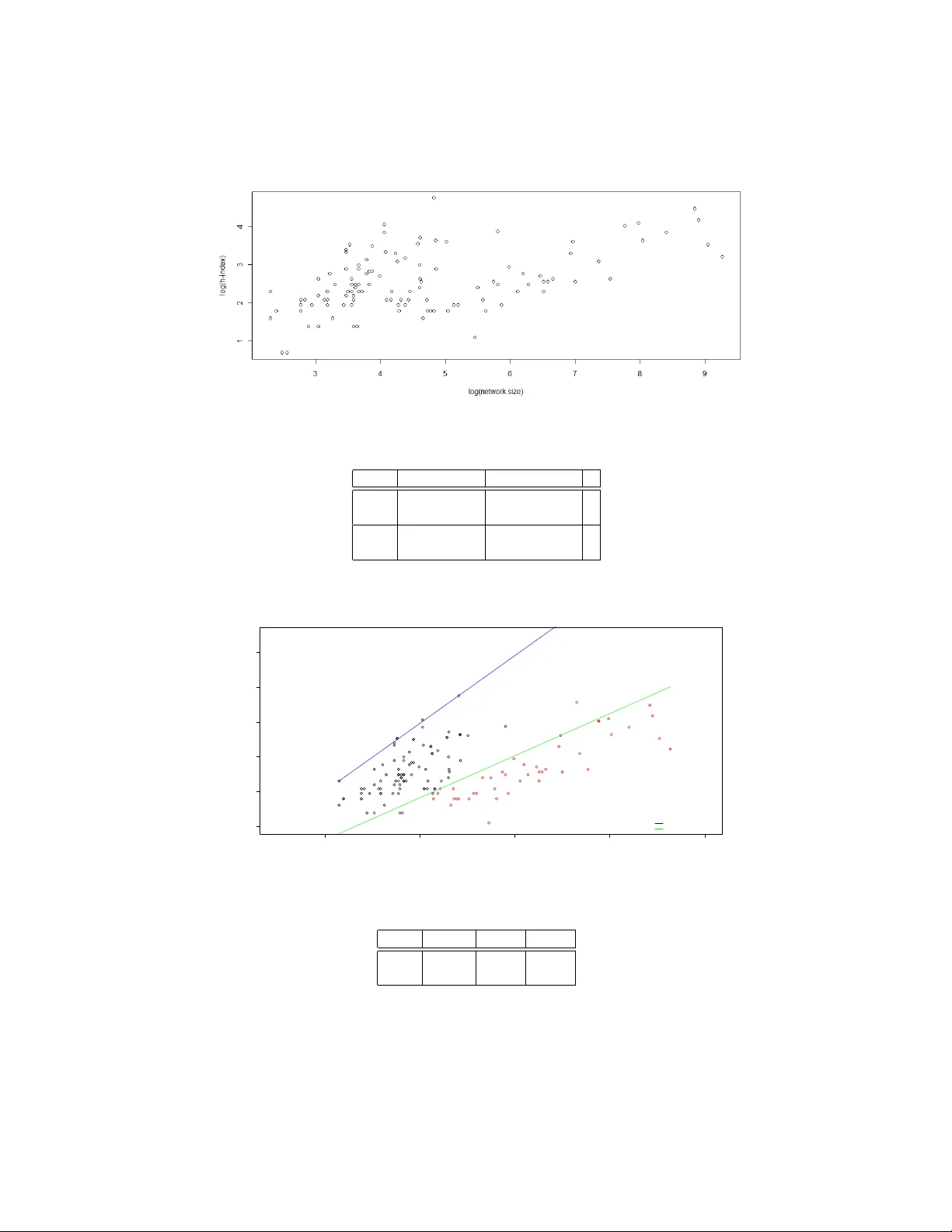
The h -Index of a Graph and its A pplication to Dynamic Subgraph Statistics David Eppstein 1 and Emma S. Spiro 2 1 Computer Science Department, Univ ersity of California, Irvine 2 Department of Sociology , Uni versity of California, Irvine Abstract. W e describe a data structure that maintains the number of triangles in a dynamic undirected graph, subject to insertions and deletions of edges and of degree-zero vertices. More generally it can be used to maintain the number of copies of each possible three-v ertex subgraph in time O ( h ) per update, where h is the h-inde x of the graph, the maximum number such that the graph contains h vertices of de gree at least h . W e also sho w ho w to maintain the h -inde x itself, and a collection of h high-degree vertices in the graph, in constant time per update. Our data structure has applications in social network analysis using the e xponen- tial random graph model (ERGM); its bound of O ( h ) time per edge is never worse than the Θ ( √ m ) time per edge necessary to list all triangles in a static graph, and is strictly better for graphs obe ying a po wer law degree distribution. In order to better understand the behavior of the h -inde x statistic and its implications for the performance of our algorithms, we also study the beha vior of the h -index on a set of 136 real-world networks. 1 Introduction The exponential random graph model (ERGM, or p ∗ model) [17, 29, 34] is a general technique for assigning probabilities to graphs that can be used both to generate sim- ulated data for social network analysis and to perform probabilistic reasoning on real- world data. In this model, one fixes the verte x set of a graph, identifies certain featur es f i in graphs on that vertex set, determines a weight w i for each feature, and sets the probability of each graph G to be proportional to an exponential function of the sum of its features’ weights, divided by a normalizing constant Z : Pr ( G ) = exp ∑ f i ∈ G w i Z . Z is found by summing over all graphs on that verte x set: Z = ∑ G exp ∑ f i ∈ G w i . For instance, if each potential edge is considered to be a feature and all edges ha ve weight ln p 1 − p , the normalizing constant Z will be ( 1 − p ) − n ( n − 1 ) / 2 , and the probability of any particular m -edge graph will be p m ( 1 − p ) n ( n − 1 ) / 2 − m , giving rise to the famil- iar Erd ˝ os-R ´ enyi G ( n , p ) model. Howe ver , the ERG model is much more general than the Erd ˝ os-R ´ enyi model: for instance, an ERGM in which the features are whole graphs can represent arbitrary probabilities. The generality of this model, and its ability to de- fine probability spaces lacking the independence properties of the simpler Erd ˝ os-R ´ enyi model, make it difficult to analyze analytically . Instead, in order to generate graphs in an ERG model or to perform other forms of probabilistic reasoning with the model, one typically uses a Marko v Chain Monte Carlo method [30] in which one performs a large sequence of small changes to sample graphs, updates after each change the counts of the number of features of each type and the sum of the weights of each feature, and uses the updated values to determine whether to accept or reject each change. Because this method must ev aluate large numbers of graphs, it is important to de velop very ef ficient algorithms for identifying the features that are present in each graph. T ypical features used in these models take the form of small subgraphs: stars of sev eral edges with a common verte x (used to represent constraints on the degree distri- bution of the resulting graphs), triangles (used in the triad model [18], an important pre- decessor of ERG models, to represent the likelihood that friends-of-friends are friends of each other), and more complicated subgraphs used to control the tendencies of sim- pler models to generate unrealistically e xtremal graphs [31]. Using highly local features of this type is important for reasons of computational efficienc y , matches well the type of data that can be obtained for real-world social networks, and is well motiv ated by the local processes believed to underly man y types of social network. Thus, ERGM simulation leads naturally to problems of subgraph isomorphism , listing or counting all copies of a giv en small subgraph in a larger graph. There has been much past algorithmic work on subgraph isomorphism problems. It is kno wn, for instance, that an n -verte x graph with m edges may have Θ ( m 3 / 2 ) triangles and four-c ycles, and all triangles and four-c ycles can be found in time O ( m 3 / 2 ) [6, 21]. All cycles of length up to seven can be counted rather than listed in time of O ( n ω ) [3] where ω ≈ 2 . 376 is the exponent from the asymptotically fastest known matrix multipli- cation algorithms [7]; this improves on the previous O ( m 3 / 2 ) bounds for dense graphs. Fast matrix multiplication has also been used for more general problems of finding and counting small cliques in graphs and hypergraphs [10, 23, 25, 33, 35]. In planar graphs, or more generally graphs of bounded local tree width, the number of copies of any fix ed subgraph may be found in linear time [13, 14], ev en though this number may be a large polynomial of the graph size [11]. Approximation algorithms for subgraph iso- morphism counting problems based on random sampling hav e also been studied, with motiv ating applications in bioinformatics [9, 22, 28]. Howe ver , much of this subgraph isomorphism research makes overly restrictiv e assumptions about the graphs that are allowed as input, runs too slowly for the ERGM application, depends on impractically complicated matrix multiplication algorithms, or does not capture the precise subgraph counts needed to accurately perform Markov Chain Monte Carlo simulations. Markov Chain Monte Carlo methods for ERGM-based reasoning process a se- quence of graphs each differing by a small change from a previous graph, so it is natural to seek additional efficienc y by applying dynamic graph algorithms [15, 16, 32], data structures to efficiently maintain properties of a graph subject to vertex and edge inser - tions and deletions. Howe ver , past research on dynamic graph algorithms has focused on problems of connectivity , planarity , and shortest paths, and not on finding the fea- 2 tures needed in ERGM calculations. In this paper , we apply dynamic graph algorithms to subgraph isomorphism problems important in ERGM feature identification. T o our knowledge, this is the first w ork on dynamic algorithms for subgraph isomorphism. A ke y ingredient in our algorithms is the h -index, a number introduced by Hirsch [20] as a way of balancing prolixity and impact in measuring the academic achiev ements of individual researchers. Although problematic in this application [1], the h -index can be defined and studied mathematically , in graph-theoretic terms, and provides a con- venient measure of the uniformity of distribution of edges in a graph. Specifically , for a researcher , one may define a bipartite graph in which the vertices on one side of the bipartition represent the researcher’ s papers, the vertices on the other side represent oth- ers’ papers, and edges correspond to citations by others of the researcher’ s papers. The h -index of the researcher is the maximum number h such that at least h vertices on the researcher’ s side of the bipartition each have degree at least h . W e generalize this to arbitrary graphs, and define the h -index of an y graph to be the maximum h such that the graph contains h vertices of degree at least h . Intuitiv ely , an algorithm whose running time is bounded by a function of h is capable of tolerating arbitrarily many low-de gree vertices without slo wdo wn, and is only mildly af fected by the presence of a small num- ber of very high degree vertices; its running time depends primarily on the numbers of intermediate-degree vertices. As we describe in more detail in Section 7, the h -inde x of any graph with m edges and n vertices is sandwiched between m / n and √ 2 m , so it is sublinear whenever the graph is not dense, and the worst-case graphs for these bounds hav e an unusual degree distrib ution that is unlikely to arise in practice. Our main result is that we may maintain a dynamic graph, subject to edge insertions, edge deletions, and insertions or deletions of isolated vertices, and maintain the number of triangles in the graph, in time O ( h ) per update where h is the h -index of the graph at the time of the update. This compares fa vorably with the time bound of Θ ( m 3 / 2 ) necessary to list all triangles in a static graph. In the same O ( h ) time bound per update we may more generally maintain the numbers of three-vertex induced subgraphs of each possible type, and in constant time per update we may maintain the h -index itself. Our algorithms are randomized, and our analysis of them uses amortized analysis to bound their expected times on worst-case input sequences. Our use of randomization is limited, howe ver , to the use of hash tables to store and retrie ve data associated with keys in O ( 1 ) expected time per access. By using either direct addressing or deterministic integer searching data structures instead of hash tables we may avoid the use of randomness at an expense of either increased space complexity or an additional factor of O ( log log n ) in time complexity; we omit the details. W e also study the behavior of the h -index, both on scale-free graph models and on a set of real-world graphs used in social network analysis. W e show that for scale-free graphs, the h -index scales as a power of n , less than its square root, while in the real- world graphs we studied the scaling exponent appears to ha ve a bimodal distrib ution. 2 Dynamic h -Indexes of Integer Functions W e begin by describing a data structure for the following problem, which generalizes that of maintaining h -indexes of dynamic graphs. W e are giv en a set S , and a function 3 f from S to the non-negati ve integers, both of which may vary discretely through a sequence of updates: we may insert or delete elements of S (with arbitrary function values for the inserted elements), and we may make arbitrary changes to the function value of any element of S . As we do so, we wish to maintain a set H such that, for ev ery x ∈ H , f ( x ) ≥ | H | , with H as large as possible with this property . W e call | H | the h-index of S and f , and we call the partition of S into the two subsets ( H , S \ H ) an h-partition of S and f . T o do so, we maintain the follo wing data structures: – A dictionary F mapping each x ∈ S to its v alue under f : F [ x ] = f ( x ) . – The set H (stored as a dictionary mapping members of H to an arbitrary value). – The set B = { x ∈ H | f ( x ) = | H |} . – A dictionary C mapping each non-negati ve integer i to the set { x ∈ S \ B | f ( x ) = i } . W e only store these sets when they are non-empty , so the situation that there is no x with f ( x ) = i can be detected by the absense of i among the keys of C . T o insert an element x into our structure, we first set F [ x ] = f ( x ) , and add x to C [ f ( x )] (or add a new set { x } at C [ f ( x )] if there is no existing entry for f ( x ) in C ). Then, we test whether f ( x ) > | H | . If not, the h -index does not change, and the insertion operation is complete. But if f ( x ) > | H | , we must include x into H . If B is nonempty , we choose an arbitrary y ∈ B , remove y from B and from H , and add y to C [ | H | ] (or create a ne w set { y } if there is no entry for | H | in C ). Finally , if f ( x ) > | H | and B is empty , the insertion causes the h -index ( | H | ) to increase by one. In this case, we test whether there is an entry for the new v alue of | H | in C . If so, we set B to equal the identity of the set in C [ | H | ] and delete the entry for | H | in C ; otherwise, we set B to the empty set. T o remove x from our structure, we remov e its entry from F and we remove it from B (if it belongs there) or from the appropriate set in C [ f ( x )] otherwise. If x did not belong to H , the h -index does not change, and the deletion operation is complete. Otherwise, let h be the v alue of | H | before remo ving x . W e remov e x from H , and attempt to restore the lost item from H by moving an element from C [ h ] to B (deleting C [ h ] if this operation causes it to become empty). But if C has no entry for h , the h -index decreases; in this case we store the identity of set B into C [ h ] , and set B to be the empty set. Changing the value of f ( x ) may be accomplished by deleting x and then reinserting it, with some care so that we do not update H if x was already in H and both the old and new v alues of f ( x ) are at least equal to | H | . Theorem 1. The data structure described above maintains the h-index of S and f , and an h-partition of S and f , in constant time plus a constant number of dictionary opera- tions per update. W e defer the proof to an appendix. 3 Gradual Appr oximate h -Partitions Although the vector h -inde x data structure of the pre vious section allo ws us to maintain the h -index of a dynamic graph very efficiently , it has a property that would be unde- sirable were we to use it directly as part of our later dynamic graph data structures: 4 the h -partition ( H , S \ H ) changes too frequently . Changes to the set H will turn out to be such an expensiv e operation that we only wish them to happen, on average, O ( 1 / h ) times per update. In order to achiev e such a small amount of change to H , we need to restrict the set of updates that are allowed: now , rather than arbitrary changes to f , we only allow it to be incremented or decremented by a single unit, and we only allow an element x to be inserted or deleted when f ( x ) = 0. W e now describe a modification of the H -partition data structure that has this property of changing more gradually for this restricted class of updates. Specifically , along with all of the structures of the H -partition, we maintain a set P ⊂ H describing a partition ( P , S \ P ) . When an element of x is removed from H , we remov e it from P as well, to maintain the in variant that P ⊂ H . Howe ver , we only add an element x to P when an update (an increment of f ( x ) or decrement of f ( y ) for some other element y ) causes f ( x ) to become greater than or equal to 2 | H | . The elements to be added to P on each update may be found by maintaining a dictionary , parallel to C , that maps each integer i to the set { x ∈ H \ P | f ( x ) = i } . Theorem 2. Let σ denote a sequence of oper ations to the data structur e described above, starting fr om an empty data structur e. Let h t denote the value of h after t op- erations, and let q = ∑ i 1 / h i . Then the data structure under goes O ( q ) additions and r emovals of an element to or fr om P. W e defer the proof to an appendix. For our later application of this technique as a subroutine in our triangle-finding data structure, we will need a more local analysis. W e may divide a sequence of updates into epochs , as follows: each epoch begins when the h -index reaches a value that differs from the value at the beginning of the previous epoch by a factor of two or more. Then, by Lemma 1, an epoch with h as its initial h -index lasts for at least Ω ( h 2 ) steps. Due to this length, we may assign a full unit of credit to each member of P at the start of each epoch, without changing the asymptotic behavior of the total number of credits assigned ov er the course of the algorithm. W ith this modification, it follows from the same analysis as above that, within an epoch of s steps, with an h -index of h at the start of the epoch, there are O ( s / h ) changes to P . 4 Counting T riangles W e are now ready to describe our data structure for maintaining the number of triangles in a dynamic graph. It consists of the following information: – A count of the number of triangles in the current graph – A set E of the edges in the graph, indexed by the pair of endpoints of the edge, allowing constant-time tests for whether a giv en pair of endpoints are linked by an edge. – A partition of the graph vertices into two sets H and V \ H as maintained by the data structure from Section 3. – A dictionary P mapping each pair of vertices u , v to a number P [ u , v ] , the number of two-edge paths from u to v via a vertex of V \ H . W e only maintain nonzero v alues for this number in P ; if there is no entry in P for the pair u , v then there exist no two-edge paths via V \ H that connect u to v . 5 Theorem 3. The data structur e described above r equir es space O ( mh ) and may be maintained in O ( h ) randomized amortized time per operation, where h is the h-index of the graph at the time of the operation. Pr oof. Insertion and deletion of vertices with no incident edges requires no change to most of these data structures, so we concentrate our description on the edge insertion and deletion operations. T o update the count of triangles, we need to kno w the number of triangles uvw in volving the edge uv that is being deleted or inserted. Triangles in which the third verte x w belongs to H may be found in time O ( h ) by testing all members of H , using the data structure for E to test in constant time per member whether it forms a triangle. T riangles in which the third verte x w does not belong to H may be counted in time O ( 1 ) by a single lookup in P . The data structure for E may be updated in constant time per operation, and the partition into H and V \ H may be maintained as described in the previous sections in constant time per operation. Thus, it remains to describe how to update P . If we are inserting an edge uv , and u does not belong to H , it has at most 2 h neighbors; we examine all other neighbors w of u and for each such neighbor increment the counter in P [ v , w ] (or create a ne w entry in P [ v , w ] with a count of 1 if no such entry already e xists). Similarly if v does not belong to H we examine all other neighbors w of v and for each such neighbor increment P [ u , w ] . If we are deleting an edge, we similarly decrement the counters or remove the entry for a counter if decrementing it would leav e a zero value. Each update in volv es incrementing or decrementing O ( h ) counters and therefore may be implemented in O ( h ) time. Finally , a change to the graph may lead to a change in H , which must be reflected in P . If a verte x v is mov ed from H to V \ H , we examine all pairs u , w of neighbors of v and increment the corresponding counts in P [ u , w ] , and if a verte x v is mov ed from V \ H to H we examine all pairs u , w of neighbors of v and decrement the corresponding counts in P [ u , w ] . This step takes time O ( h 2 ) , because v has O ( h ) neighbors when it is moved in either direction, but as per the analysis in Section 3 it is performed an av erage of O ( 1 / h ) times per operation, so the amortized time for updates of this type, per change to the input graph, is O ( h ) . The space for the data structure is O ( m ) for E , O ( n ) for the data structure that maintains H , and O ( mh ) for P because each edge of the graph belongs to O ( h ) two- edge paths through low-de gree vertices. u t 5 Subgraph Multiplicity Although the data structure of Theorem 3 only counts the number of triangles in a graph, it is possible to use it to count the number of three-v ertex subgraphs of all types, or the number of induced three-vertex subgraphs of all types. In what follows we let p i = p i ( G ) denote the number of paths of length i in G , and we let c i = c i ( G ) denote the number of cycles of length i in G . The set of all edges in a graph G among a subset of three vertices { u , v , w } determine one of four possible induced subgraphs: an independent set with no edges, a graph with 6 a single edge, a two-star consisting of two edges, or a triangle. Let g 0 , g 1 , g 2 , and g 3 denote the numbers of three-vertex subgraphs of each of these types, where g i counts the three-verte x induced subgraphs that hav e i edges. Observe that it is trivial to maintain for a dynamic graph, in constant time per oper- ation, the three quantities n , m , and p 2 , where n denotes the number of vertices of the graph, m denotes the number of edges, and p 2 denotes the number of two-edge paths that can be formed from the edges of the graph. Each change to the graph increments or decrements n or m . Additionally , adding an edge uv to a graph where u and v already hav e d u and d v incident edges respectively increases p 2 by d u + d v , while removing an edge uv decreases p 2 by d u + d v − 2. Letting c 3 denote the number of triangles in the graph as maintained by Theorem 3, the quantities described above satisfy the matrix equation     1 1 1 1 0 1 2 3 0 0 1 3 0 0 0 1         g 0 g 1 g 2 g 3     =     n ( n − 1 )( n − 2 ) / 6 m ( n − 2 ) p 2 c 3     . Each row of the matrix corresponds to a single linear equation in the g i values. The equation from the first row , g 0 + g 1 + g 2 + g 3 =  n 3  , can be interpreted as stating that all triples of vertices form one graph of one of these types. The equation from the second row , g 1 + 2 g 2 + 3 g 3 = m ( n − 2 ) , is a form of double counting where the number of edges in all three-vertex subgraphs is added up on the left hand side by subgraph type and on the right hand side by counting the number of edges ( m ) and the number of triples each edge participates in ( n − 2). The third row’ s equation, g 2 + 3 g 3 = p 2 , similarly counts incidences between two-edge paths and triples in two ways, and the fourth equation g 3 = c 3 follows since each three vertices that are connected in a triangle cannot form any other induced subgraph than a triangle itself. By in verting the matrix we may reconstruct the g values: g 3 = c 3 g 2 = p 2 − 3 g 3 g 1 = m ( n − 2 ) − ( 2 g 2 + 3 g 3 ) g 0 =  n 3  − ( g 1 + g 2 + g 3 ) . Thus, we may maintain each number of induced subgraphs g i in the same asymptotic time per update as we maintain the number of triangles in our dynamic graph. The numbers of subgraphs of dif ferent types that are not necessarily induced are even easier to recover: the number of three-vertex subgraphs with i edges is given by the i th entry of the vector on the right hand side of the matrix equation. As we detail in an appendix, it is also possible to maintain efficiently the numbers of star subgraphs of a dynamic graph, and the number of four -verte x paths in a dynamic graph. 7 6 W eighted Edges and Colored V ertices It is possible to generalize our triangle counting method to problems of weighted trian- gle counting: we assign each edge uv of the graph a weight w uv , define the weight of a triangle to be the product of the weights of its edges, and maintain the total weight of all triangles. For instance, if 0 ≤ w uv ≤ 1 and each edge is present in a subgraph with probability w uv , then the total weight gi ves the expected number of triangles in that subgraph. Theorem 4. The total weight of all triangles in a weighted dynamic graph, as de- scribed above, may be maintained in time O ( h ) per update. Pr oof. W e modify the structure P [ u , v ] maintained by our triangle-finding data structure, so that it stores the weight of all two-edge paths from u to v . Each update of an edge uv in our structure in volv es a set of indi vidual triangles uvx in volving vertices x ∈ H (whose weight is easily calculated) together with the triangles formed by paths counted in P [ u , v ] (whose total weight is P [ u , v ] w uv ). The same time analysis from Theorem 3 holds for this modified data structure. u t For social networking ERGM applications, an alternati ve generalization may be ap- propriate. Suppose that the vertices of the giv en dynamic graph are colored; we wish to maintain the number of triangles with each possible combination of colors. For instance, in graphs representing sexual contacts [24], edges between individuals of the same sex may be less frequent than edges between indi viduals of opposite sexes; one may model this in an ERGM by assigning the vertices two different colors according to whether they represent male or female individuals and using feature weights that depend on the colors of the vertices in the features. As we now show , problems of counting colored triangles scale well with the number of different groups into which the vertices of the graph are classified. Theorem 5. Let G be a dynamic graph in which each vertex is assigned one of k dif- fer ent colors. Then we may maintain the numbers of triangles in G with each possible combination of colors, in time O ( h + k ) per update. Pr oof. W e modify the structure P [ u , v ] stored by our triangle-finding data structure, to store a vector of k numbers: the i th entry in this v ector records the number of two- edge paths from u to v through a low-de gree verte x with color i . Each update of an edge uv in our structure inv olves a set of individual triangles uvx in v olving vertices x ∈ H (whose colors are easily observed) together with the triangles formed by paths counted in P [ u , v ] (with k dif ferent possible colorings, recorded by the entries in the vector P [ u , v ] ). Thus, the part of the update operation in which we compute the numbers of triangles for which the third verte x has lo w degree, by looking up u and v in P , takes time O ( k ) instead of O ( 1 ) . The same time analysis from Theorem 3 holds for all other aspects of this modified data structure. u t Both the weighting and coloring generalizations may be combined with each other without loss of efficienc y . 8 7 How Small is the h -Index of T ypical Graphs? It is straightforward to identify the graphs with extremal values of the h -index. A split graph in which an h -vertex clique is augmented by adding n − h vertices, each connected only to the vertices in the clique, has n vertices and m = h ( n − 1 ) edges, achieving an h -index of m / ( n − 1 ) . This is the minimum possible among any graph with n vertices and m edges: any other graph may be transformed into a split graph of this type, while increasing its number of edges and not decreasing h , by finding an h -partition ( H , V \ H ) and repeatedly replacing edges that do not ha ve an endpoint in H by edges that do hav e such an endpoint. The graph with the largest h -index is a clique with m edges together with enough isolated vertices to fill out the total to n ; its h -index is √ 2 m ( 1 + o ( 1 )) . Thus, for sparse graphs in which the numbers of edges and vertices are proportional to each other , the h -index may be as small as O ( 1 ) or as large as Ω ( √ n ) . At which end of this spectrum can we expect to find the graphs arising in social network analysis? One answer can be provided by fitting mathematical models of the de gr ee distribu- tion , the relation between the number of incident edges at a vertex and the number of vertices with that many edges, to social networks. For many large real-world graphs, observers have reported power laws in which the number of vertices with degree d is proportional to nd − γ for some constant γ > 1; a network with this property is called scale-fr ee [2, 24, 26, 27]. T ypically , γ lies in or near the interval 2 ≤ γ ≤ 3 although more extreme values are possible. The h -index of these graphs may be found by solving for the h such that h = nh − γ ; that is, h = Θ ( n 1 / ( 1 + γ ) ) . For any γ > 1 this is an asymptotic improv ement on the worst-case O ( √ n ) bound for graphs without po wer-law degree distributions. For instance, for γ = 2 this would giv e a bound of h = O ( n 1 / 3 ) while for γ = 3 it would give h = O ( n 1 / 4 ) . That is, by depending on the h -index as it does, our algorithm is capable of taking advantage of the extra structure inherent in scale-free graphs to run more quickly for them than it does in the general case. T o further explore h -index behavior in real-world networks, we computed the h - index for a collection of 136 network data sets typical of those used in social network analysis. These data sets were drawn from a variety of sources traditionally viewed as common repositories for such data. The majority of our data sets were from the well known P ajek datasets [4]. Pajek is a program used for the analysis and visualization of large networks. The collection of data available with the Pajek software includes cita- tion networks, food-webs, friendship network, etc. In addition to the Pajek data sets, we included network data sets from UCINET [5]. Another software package de veloped for network analysis, UCINET includes a corpus of data sets that are more traditional in the social sciences. Many of these data sets represent friendship or communication rela- tions; UCINET also includes various social networks for non-human animals. W e also used network data included as part of the statnet software suite [19], statistical model- ing software in R. statnet includes ERGM functionality , making it a good example for data used specifically in the context of ERG models. Finally , we included data a vailable on the UCI Network Data Repository [8], including some larger networks such as the WWW , blog networks, and other online social networks. By using this data we hope to understand how the h -index scales in real-world networks. Details of the statistics for these networks are presented in an appendix; a summary of the statistics for network size and h -index are in T able 1, below . For this sample of 9 136 real-w orld networks, the h -inde x ranges from 2 to 116. The ro w of summary statis- tics for log h / log n suggests that, for man y netw orks, h scales as a sublinear po wer of n . The one case with an h -index of 116 represents the ties among Slovenian magazines and journals between 1999 and 2000. The vertices of this network represent journals, and undirected edges between journals have an edge weight that represents the num- ber of shared readers of both journals; this network also includes self-loops describing the number of all readers that read this journal. Thus, this is a dense graph, more ap- propriately handled using statistics in volving the edge weights than with combinatorial techniques in volving the existence or nonexistence of triangles. Howe ver , this is the only network from our dataset with an h -inde x in the hundreds. Ev en with significantly larger netw orks, the h -index appears to scale sublinearly in most cases. min. median mean max. network size ( n ) 10 67 535.3 10616 h -index ( h ) 2 12 19.08 116 log n 2.303 4.204 4.589 9.270 log h 0.6931 2.4849 2.6150 4.7536 log h / log n 0.2014 0.6166 0.6006 1.0000 T able 1. Summary statistics for real-world network data A histogram of the h -index data in Figure 1 clearly shows a bimodal distribution. Additionally , as the second peak of the bimodal distribution corresponds to a scaling exponent greater than 0.5, the graphs corresponding to that peak do not match the pre- dictions of the scale-free model. Howe ver we were unable to discern a pattern to the types of networks with smaller or larger h -indices, and do not speculate on the reasons for this bimodality . W e look more deeply at the scaling of the h -index using standard regression techniques in an appendix. Fig. 1. A frequency histogram for log h / log n . 10 8 Discussion W e have defined an interesting new graph in v ariant, the h -index, presented ef ficient dynamic graph algorithms for maintaining the h -index and, based on them, for main- taining the set of triangles in a graph, and studied the scaling behavior of the h -index both on theoretical scale-free graph models and on real-world network data. There are many directions for future work. For sparse graphs, the h -index may be larger than the arboricity , a graph in v ariant used in static subgraph isomorphism [6, 12]; can we speed up our dynamic algorithms to run more quickly on graphs of bounded arboricity? W e handle undirected graphs but the directed case is also of interest. W e would like to find ef ficient data structures to count lar ger subgraphs such as 4-c ycles, 4- cliques, and claws; dynamic algorithms for these problems are likely to be slower than our triangle-finding algorithms but may still provide speedups ov er static algorithms. Another network statistic related to triangle counting is the clustering coefficient of a graph; can we maintain it efficiently? Additionally , there is an opportunity for additional work in implementing our data structures and testing their ef ficiency in practice. Acknowledgements This work was supported in part by NSF grant 0830403 and by the Office of Na v al Research under grant N00014-08-1-1015. References 1. R. Adler , J. Ewing, and P . T aylor . Citation Statistics: A report fr om the International Mathematical Union (IMU) in cooperation with the International Council of Industrial and Applied Mathematics (ICIAM) and the Institute of Mathematical Statistics . Joint Committee on Quantitativ e Assessment of Research, 2008. 2. R. Albert, H. Jeong, and A.-L. Barabasi. The diameter of the world wide web. Natur e , 401:130–131, 1999. 3. N. Alon, R. Y uster, and U. Zwick. Finding and counting given length c ycles. Algorithmica , 17(3):209–223, 1997. 4. V . Batagelj and A. Mrv ar . Pajek datasets. W eb page http://vlado.fmf.uni-lj.si/pub/networks/data/, 2006. 5. S. P . Borgatti, M. G. Everett, and L. C. Freeman. UCINet 6 for W indows: Software for social network analysis . Analytic T echnologies, Harvard, MA, 2002. 6. N. Chiba and T . Nishizeki. Arboricity and subgraph listing algorithms. SIAM Journal on Computing , 14(1):210–223, 1985. 7. D. Coppersmith and S. W inograd. Matrix multiplication via arithmetic progressions. Journal of Symbolic Computation , 9(3):251–280, 1990. 8. C. L. DuBois and P . Smyth. UCI Network Data Repository. W eb page http://networkdata.ics.uci.edu, 2008. 9. R. A. Duke, H. Lefmann, and V . R ¨ odl. A fast approximation algorithm for computing the frequencies of subgraphs in a giv en graph. SIAM Journal on Computing , 24(3):598–620, 1995. 10. F . Eisenbrand and F . Grandoni. On the complexity of fixed parameter clique and dominating set. Theoretical Computer Science , 326(1–3):57–67, 2004. 11. D. Eppstein. Connectivity , graph minors, and subgraph multiplicity. Journal of Graph Theory , 17:409–416, 1993. 11 12. D. Eppstein. Arboricity and bipartite subgraph listing algorithms. Information Processing Letters , 51(4):207–211, August 1994. 13. D. Eppstein. Subgraph isomorphism in planar graphs and related problems. Journal of Graph Algorithms & Applications , 3(3):1–27, 1999. 14. D. Eppstein. Diameter and treewidth in minor-closed graph f amilies. Algorithmica , 27:275–291, 2000. 15. D. Eppstein, Z. Galil, and G. F . Italiano. Dynamic graph algorithms. In M. J. Atallah, editor , Algorithms and Theory of Computation Handbook , chapter 8. CRC Press, 1999. 16. J. Feigenbaum and S. Kannan. Dynamic graph algorithms. In K. Rosen, editor, Handbook of Discr ete and Combinatorial Mathematics . CRC Press, 2000. 17. O. Frank. Statistical analysis of change in networks. Statistica Neerlandica , 45:283–293, 199. 18. O. Frank and D. Strauss. Markov graphs. Journal of the American Statistical Association , 81:832–842, 1986. 19. M. S. Handcock, D. Hunter , C. T . Butts, S. M. Goodreau, and M. Morris. statnet: An R package for the Statistical Modeling of Social Networks. W eb page http://www .csde.washington.edu/statnet, 2003. 20. J. E. Hirsch. An index to quantify an individual’ s scientific research output. Pr oc. National Academy of Sciences , 102(46):16569–16572, 2005. 21. A. Itai and M. Rodeh. Finding a minimum circuit in a graph. SIAM Journal on Computing , 7(4):413–423, 1978. 22. N. Kashtan, S. Itzkovitz, R. Milo, and U. Alon. Efficient sampling algorithm for estimating subgraph concentrations and detecting network motifs. Bioinformatics , 20(11):1746–1758, 2004. 23. T . Kloks, D. Kratsch, and H. M ¨ uller . Finding and counting small induced subgraphs efficiently. Information Pr ocessing Letters , 74(3–4):115–121, 2000. 24. F . Liljeros, C. R. Edling, L. A. N. Amaral, H. E. Stanley , and Y . ˚ Aberg. The web of human sexual contacts. Nature , 411:907–908, 2001. 25. J. Ne ˇ set ˇ ril and S. Poljak. On the complexity of the subgraph problem. Commentationes Mathematicae Universitatis Car olinae , 26(2):415–419, 1985. 26. M. E. J. Newman. The structure and function of complex networks. SIAM Review , 45:167–256, 2003. 27. D. J. d. S. Price. Networks of scientific papers. Science , 149(3683):510–515, 1965. 28. N. Pr ˇ zulj, D. G. Corneil, and I. Jurisica. Efficient estimation of graphlet frequency distributions in protein–protein interaction netw orks. Bioinformatics , 22(8):974–980, 2006. 29. G. Robins and M. Morris. Advances in exponential random graph ( p ∗ ) models. Social Networks , 29(2):169–172, 2007. Special issue of journal with four additional articles. 30. T . A. B. Snijders. Markov chain Monte Carlo estimation of e xponential random graph models. Journal of Social Structure , 3(2):1–40, 2002. 31. T . A. B. Snijders, P . E. Pattison, G. Robins, and M. S. Handcock. New specifications for exponential random graph models. Sociological Methodology , 36(1):99–153, 2006. 32. M. Thorup and D. R. Karger . Dynamic graph algorithms with applications. In Proc. 7th Scandinavian W orkshop on Algorithm Theory (SW A T 2000) , volume 1851 of Lectur e Notes in Computer Science , pages 667–673. Springer-V erlag, 2000. 33. V . V assilevska and R. W illiams. Finding, minimizing and counting weighted subgraphs. In Pr oc. 41st ACM Symposium on Theory of Computing , 2009. 34. S. W asserman and P . E. Pattison. Logit models and logistic regression for social networks, I: an introduction to Markov graphs and p ∗ . Psychometrika , 61:401–425, 1996. 35. R. Y uster . Finding and counting cliques and independent sets in r -uniform hypergraphs. Information Pr ocessing Letters , 99(4):130–134, 2006. 12 A ppendix I: Proof of Theorems 1 and 2 W e begin by proving Theorem 1, the correctness of our data structure for maintaining the h -index and h -partition, and the analysis showing that it takes constant time per operation. Pr oof. The time analysis follows immediately from the description of the data structure update operations. These updates maintain inv ariant the properties of the set B and the dictionary of sets C [ i ] that they partition S properly by their values of f ( x ) , that B consists exactly of those elements of H with f ( x ) = | H | , and that H consists of B together with those elements of S with f ( x ) > | H | . Thus, h = | H | has the property that there exists a set (namely H ) with h elements, all of which have function v alue at least h . There can be no larger h 0 with the same property , because all of the elements with value greater than h belong to H already so there can be no larger set of elements with larger values. Thus, h is the correct h -index of S and f , and ( H , S \ H ) is a correct h -partition. u t Next we prov e Theorem 2, the time analysis of our data structure for maintaining a partition of a graph into lo w and high degree vertices with a very low number of mov es of vertices from one part of the partition to the other . As an accounting technique for the analysis of the algorithm (not something actu- ally stored within our data structure) we associate a (fractional) number of “credits” with each member of P , that is zero when that element is added to P . Each increment operation adds 1 / | H | 2 credit to each current member of P , and each decrement opera- tion on a member of P adds 1 / | H | credits to that member . Lemma 1. Any sequence of operations during which | H | chang es fr om h to h 0 > h includes at least ( h 0 − h ) 2 incr ement operations. Pr oof. There exist at least h 0 − h members of the set H after the sequence that were not members prior to the sequence. Each of these elements has f ( x ) ≤ h prior to the sequence (else it would belong to H ) and f ( x ) ≥ h 0 after the sequence, so the number of increments for these elements alone must hav e been at least ( h 0 − h ) 2 . u t Lemma 2. Any element x that is remo ved fr om P must have accumulated Ω ( 1 ) credits. Pr oof. Let h be the v alue of | H | at the time x was added to P , and h 0 be the v alue of max ( h , | H | ) at the time it is remov ed. Then by the previous lemma, x must hav e accumulated ( h 0 − h ) 2 / h 2 credits from increment operations, and Ω (( 2 h − h 0 ) / h ) credits from decrement operations. But for an y h 0 ≥ h , ( h 0 − h ) 2 / h 2 + ( 2 h − h 0 ) / h = Ω ( 1 ) . u t The proof of Theorem 2 now follo ws. Pr oof. The number of additions is equal to the number of remo vals, plus the number of items that remain in H at the end of the sequence. But by Lemma 1 we can find a sub- sequence I of increase operations such that the final v alue of | H | is O ( ∑ i ∈ I 1 / h i ) . Thus, we need count only the number of times elements are removed from P . By Lemma 2, this number of removals is proportional to the total number of credits that hav e been accumulated by all elements o ver the course of σ . But, since each operation assigned at most 1 / h i credits, this total is at most q . u t 13 A ppendix II: Additional subgraph counting data structures If s i = s i ( G ) denote the number of star subgraphs K 1 , i in G , we may maintain s i , for any constant i , in constant time per update, as it is a sum of polynomials of the vertex degrees: s i = ∑ v d v ( d v − 1 ) · · · ( d v − i − 1 ) / i !. For instance, the number of claws (three- leaf stars) in G is s 3 = ∑ v d v ( d v − 1 )( d v − 2 ) / 6. In at least one other nontrivial case we may maintain the number of four-verte x subgraphs of a certain type as efficiently as the number of triangles. Theorem 6. W e may maintain a dynamic graph subject to edge insertions and deletions and to insertions and deletions of isolated vertices, and keep trac k of the number p 3 of four-verte x paths in the graph, in amortized time O ( h ) per update where h is the h-index of the graph at the time of an update. Pr oof. Let q denote the number of sequences of three edges that form either a path or a cycle in G . Let d v denote the degree of v (that is, its number of incident edges), and let P v denote the number of two-edge paths having v as an endpoint (that is, ∑ ( d w − 1 ) where the sum is ov er all neighbors of v in G ). Inserting an edge uv into the graph G increases q by d u d v + P u + P v : the term d u d v counts the paths with uv as middle edge, and the other two terms count the paths ha ving v or u as endpoint. Similarly , remo ving edge uv decreases q by ( d u − 1 )( d v − 1 ) + ( P u − d v + 1 ) + ( P v − d u + 1 ) . Thus, if we can calculate P u and P v , we can correctly update q . Our data structure stores the numbers d v for each vertex v , and the numbers P u only for those vertices u that belong to the set H maintained by the gradual partition of Section 3. When a vertex is added to H , the value P u stored for it may be computed in time O ( h ) . When we insert or delete an edge uv , the numbers P u and P v that we need to use to update q may be found either by looking them up in this data structure (if the endpoints u or v of the updated edge belong to H ) or in time O ( h ) by looking at all neighbors of the endpoints if they do not belong to H . Finally , whenev er we insert or delete an edge uv , we must update the numbers P w for all vertices w belonging to H , where either w is one of the two endpoints u and v or it is adjacent to one or both of these endpoints; this update may be performed in constant time per member of H , or O ( h ) time total. The number of four-verte x paths that we maintain is then p 3 = q − 3 c 3 where c 3 denotes the number of triangles in the graph as maintained by our other structures. u t The counts of larger subgraphs in G obey additional linear relations: for instance, ∑ v P 2 v = p 4 + 2 p 2 + 3 s 3 + 4 c 4 . Ho we ver we ha ve not been able to e xploit these relations by finding efficient algorithms for maintaining the quantities p 4 and c 4 . 14 A ppendix III: Detailed analysis of real-world network data W e calculated the h -index of the networks in our sample in R, using a subroutine pro- vided by Carter Butts. The data that results from this calculation in plotted in Figure 2. Fig. 2. Scatter plot of h -index and network size Figure 2 suggests that the data might be more appropriately viewed on a log-log scale. This plot is seen in Figure 3. 8.1 Quantile regr ession T o find an upper bound on the scaling of the h -index of our real world networks we clustered the data into two groups, and used quantile regression to fit the data with curves of the form log h = β 0 + β 1 log n , at the 95th percentile. That is, we are looking for a power law h = cn β 1 , and we want 95% of the graphs to have an h -index no larger than the one predicted by this law . W e fit a law of this type to the tw o clusters separately to provide a more conservati v e and substantive prediction. The resulting regression lines are reported in T able 2. Corresponding goodness of fit measure are also reported in T able 3. W e note that these are conservati ve estimates and the actual scaling is likely better . 15 Fig. 3. Scatter plot of h -index and network size, on log-log scale Cluster Intercept β 0 Slope β 1 df 1 0.0609 0.9735 92 (-0.964, 2.581) (0.231, 1.266) 2 -0.598 0.604 44 (-1.938, 5.248) (0.44712, 0.847) T able 2. Coefficients for quantile re gression lines ● ● ● ● ● ● ● ● ● ● ● ● ● ● ● ● ● ● ● ● ● ● ● ● ● ● ● ● ● ● ● ● ● ● ● ● ● ● ● ● ● ● ● ● ● ● ● ● ● ● ● ● ● ● ● ● ● ● ● ● ● ● ● ● ● ● ● ● ● ● ● ● ● ● ● ● ● ● ● ● ● ● ● ● ● ● ● ● ●● ● ● ● ● ● ● ● ● ●● ● ● ● ● ● ● ● ● ● ● ● ● ● ● ● ● ● ● ● ● ● ● ● ● ● ● ● ● ● ● ● ● ● ● 2 4 6 8 10 1 2 3 4 5 6 log (size) log (h−index) Cluster 1: 95th pencentile Cluster 2: 95th pencentile Fig. 4. H-index scaling using quantile regression fits Cluster log-like AIC BIC 1 -109.345 222.691 227.734 2 -41.071 86.143 89.712 T able 3. Goodness of fit measures for quantile regression lines 16 A ppendix IV : Raw data from analysis of real-w orld networks n h log n log h log h log n 10 5 2.3026 1.6094 0.6990 10 10 2.3026 2.3026 1.0000 11 6 2.3979 1.7918 0.7472 11 6 2.3979 1.7918 0.7472 12 2 2.4849 0.6931 0.2789 13 2 2.5649 0.6931 0.2702 16 6 2.7726 1.7918 0.6462 16 6 2.7726 1.7918 0.6462 16 8 2.7726 2.0794 0.7500 16 7 2.7726 1.9459 0.7018 17 8 2.8332 2.0794 0.7340 18 4 2.8904 1.3863 0.4796 19 7 2.9444 1.9459 0.6609 21 14 3.0445 2.6391 0.8668 21 9 3.0445 2.1972 0.7217 21 4 3.0445 1.3863 0.4553 23 8 3.1355 2.0794 0.6632 24 10 3.1781 2.3026 0.7245 24 8 3.1781 2.0794 0.6543 24 7 3.1781 1.9459 0.6123 24 7 3.1781 1.9459 0.6123 25 16 3.2189 2.7726 0.8614 26 5 3.2581 1.6094 0.4940 27 12 3.2958 2.4849 0.7540 31 7 3.4340 1.9459 0.5667 32 9 3.4657 2.1972 0.6340 32 28 3.4657 3.3322 0.9615 32 30 3.4657 3.4012 0.9814 32 18 3.4657 2.8904 0.8340 33 10 3.4965 2.3026 0.6585 34 34 3.5264 3.5264 1.0000 34 34 3.5264 3.5264 1.0000 35 10 3.5553 2.3026 0.6476 35 12 3.5553 2.4849 0.6989 n h log n log h log h log n 35 12 3.5553 2.4849 0.6989 35 7 3.5553 1.9459 0.5473 35 14 3.5553 2.6391 0.7423 35 12 3.5553 2.4849 0.6989 36 4 3.5835 1.3863 0.3869 36 9 3.5835 2.1972 0.6131 36 8 3.5835 2.0794 0.5803 37 11 3.6109 2.3979 0.6641 37 11 3.6109 2.3979 0.6641 37 12 3.6109 2.4849 0.6882 38 4 3.6376 1.3863 0.3811 39 10 3.6636 2.3026 0.6285 39 10 3.6636 2.3026 0.6285 39 12 3.6636 2.4849 0.6783 39 18 3.6636 2.8904 0.7890 39 20 3.6636 2.9957 0.8177 39 12 3.6636 2.4849 0.6783 41 10 3.7136 2.3026 0.6200 44 16 3.7842 2.7726 0.7327 44 23 3.7842 3.1355 0.8286 46 12 3.8286 2.4849 0.6490 46 17 3.8286 2.8332 0.7400 48 33 3.8712 3.4965 0.9032 48 33 3.8712 3.4965 0.9032 48 17 3.8712 2.8332 0.7319 54 15 3.9890 2.7081 0.6789 58 47 4.0604 3.8501 0.9482 58 58 4.0604 4.0604 1.0000 59 28 4.0775 3.3322 0.8172 60 8 4.0943 2.0794 0.5079 60 8 4.0943 2.0794 0.5079 62 14 4.1271 2.6391 0.6394 64 8 4.1589 2.0794 0.5000 65 10 4.1744 2.3026 0.5516 17 n h log n log h log h log n 69 27 4.2341 3.2958 0.7784 69 27 4.2341 3.2958 0.7784 69 27 4.2341 3.2958 0.7784 71 22 4.2627 3.0910 0.7251 71 22 4.2627 3.0910 0.7251 72 7 4.2767 1.9459 0.4550 73 6 4.2905 1.7918 0.4176 75 8 4.3175 2.0794 0.4816 75 8 4.3175 2.0794 0.4816 80 7 4.3820 1.9459 0.4441 80 24 4.3820 3.1781 0.7252 84 8 4.4308 2.0794 0.4693 86 10 4.4543 2.3026 0.5169 97 35 4.5747 3.5553 0.7772 97 35 4.5747 3.5553 0.7772 100 11 4.6052 2.3979 0.5207 100 20 4.6052 2.9957 0.6505 101 14 4.6151 2.6391 0.5718 101 41 4.6151 3.7136 0.8047 102 13 4.6250 2.5649 0.5546 105 5 4.6540 1.6094 0.3458 111 8 4.7095 2.0794 0.4415 112 6 4.7185 1.7918 0.3797 118 6 4.7707 1.7918 0.3756 124 116 4.8203 4.7536 0.9862 124 6 4.8203 1.7918 0.3717 128 38 4.8520 3.6376 0.7497 128 38 4.8520 3.6376 0.7497 128 38 4.8520 3.6376 0.7497 129 18 4.8598 2.8904 0.5947 151 37 5.0173 3.6109 0.7197 154 6 5.0370 1.7918 0.3557 169 7 5.1299 1.9459 0.3793 180 7 5.1930 1.9459 0.3747 n h log n log h log h log n 205 11 5.3230 2.3979 0.4505 234 3 5.4553 1.0986 0.2014 244 11 5.4972 2.3979 0.4362 265 8 5.5797 2.0794 0.3727 275 6 5.6168 1.7918 0.3190 311 13 5.7398 2.5649 0.4469 332 48 5.8051 3.8712 0.6669 332 12 5.8051 2.4849 0.4281 352 7 5.8636 1.9459 0.3319 395 19 5.9789 2.9444 0.4925 452 10 6.1137 2.3026 0.3766 489 16 6.1924 2.7726 0.4477 533 12 6.2785 2.4849 0.3958 638 15 6.4583 2.7081 0.4193 673 13 6.5117 2.5649 0.3939 674 10 6.5132 2.3026 0.3535 719 13 6.5779 2.5649 0.3899 775 14 6.6529 2.6391 0.3967 1022 27 6.9295 3.2958 0.4756 1059 37 6.9651 3.6109 0.5184 1096 13 6.9994 2.5649 0.3665 1490 96 7.3065 4.5643 0.6247 1577 22 7.3633 3.0910 0.4198 1882 14 7.5401 2.6391 0.3500 2361 56 7.7668 4.0254 0.5183 2361 56 7.7668 4.0254 0.5183 2361 56 7.7668 4.0254 0.5183 2909 60 7.9756 4.0943 0.5134 3084 38 8.0340 3.6376 0.4528 4470 47 8.4051 3.8501 0.4581 6927 88 8.8432 4.4773 0.5063 7343 65 8.9015 4.1744 0.4690 8497 34 9.0475 3.5264 0.3898 10616 25 9.2701 3.2189 0.3472 18