Modular Compilation of a Synchronous Language

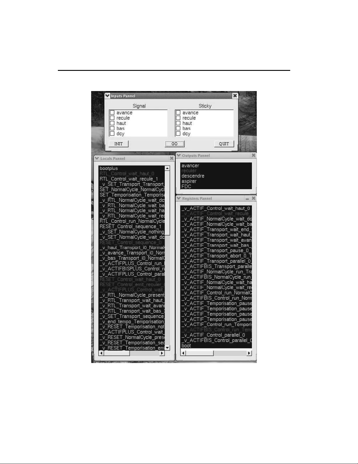
apport   de recherche ISSN 0249-6399 ISRN INRIA/RR--6424--FR+ENG Thème COG INSTITUT N A TION AL DE RECHERCHE EN INFORMA TIQUE ET EN A UTOMA TIQUE Modular Compilation of a Sync hronous Language Daniel Gaffé — Annie Ressouche — V alérie Roy N° 6424 April 25, 2022 Unité de recherche INRIA Sophia Antipolis 2004, route des Lucioles, BP 93, 06902 Sophia Antipolis Cedex (France) Téléphone : +33 4 92 38 77 77 — Téléco pie : +33 4 92 38 77 65 Modular Compilation of a Synchr onous Language Daniel Gaffé ∗ , Annie Ressouche † , V alérie Roy ‡ § Thème COG — Systèmes cogn itifs Projet Pulsar Rapport de recherche n° 6424 — April 25, 2022 — 61 pages Abstract: Synchro nous languages r ely on formal m ethods to facilitate th e d ev elope ment of app li- cations in an efﬁcient and reusable w ay . In fact, formal method s ha ve been advocated as a means of increasing the reliability of systems, especially those which are safety or business critical. I t is even more difﬁcult to de velop automatic speciﬁcation and veriﬁcation t ools du e to limitations such as state explosion, unde cidability , etc... In this work, we design a n ew speciﬁcation mod el based o n a reac- ti ve s ynch rono us approac h. W e beneﬁt from a formal framew ork well suited to per form co mpilation and forma l v alidation of systems. In practice, we design and implement a special purpose language ( L E ) wi th two sem antic: its behav ioral semantic helps u s to d eﬁne a p rogr am by the s et of its beha v- iors and avoid am biguity i n progra ms in terpretation ; its equationa l semantic allo ws the co mpilation of progr ams in to software and hardware targets (C code, Vhdl code, Fpga synthesis, Model checker input f ormat). Our approach is r elev ant with respect to the two main r equirem ents of critical realistic applications: modular compilation allows us to deal with large systems, while mo del-based approach provides us with formal validation. There is still a lack of e fﬁcient and modu lar compilation means for synchro nous languages. Despite o f r elev ant attempts to optimize g enerated code, no app roach considers modu lar compilation. Th is repor t tackles this problem by intro ducing a compilation tech- nique which relies on the equational semantic to ensure modularity completed by a ne w algorithm to check causality cycles in the whole program without checking again t he ca usalty of sub programs. Key-words: synchro nous languag e, modu lar comp ilation, beh avioral semantic, eq uational co n- structive semantic, mod ularity , separate comp ilation. ∗ I3S Laboratory and CNRS † INRIA Sophia Antipol is ‡ CMA ENM Sophia Antipol is § thanks to S. Moisan and J.P Rigault for their carefu l rea ding a nd their fruitful suggestions Compilation modulair e d’un langage synchr one Résumé : Dans ce rappor t, no us étudions le développ ement de systèmes critiques. Les méthod es formelles se sont avérées un m oyen efﬁcace pou r augm enter la ﬁabilité d e tels systèmes, en parti- culier ceux qui req uièrent une ce rtaine sécurité de fo nctionn ement. Neanmoins, le dé veloppemen t d’outils automatiqu es de spé ciﬁcation et de vér iﬁcation e st limité en tre autre par la taille des mo- dèles form els des systèmes ou par d es problèm es d’indécidab ilité. Dans ce trav ail, nous déﬁnissons un langag e ré actif synchro ne ( L E ) dédié à la spéciﬁcation d e systèmes critiq ues. Ce faisant, nous bénéﬁcion s d ’un cadre formel sur lequel no us nous ap puyo ns po ur compiler sépar ement et valider les applications. Plus précisement, nous déﬁnissons deux sémantique s p our notre langage : un e sé- mantique comportemen tale q ui associe à un pro gramm e l’ensemb le de ses comp ortements et évite ainsi toute am biguité dans l’in terpretatio n des prog rammes. Nous déﬁn issons aussi un e sémantiqu e équation nelle dirigeant la compilation de prog rammes vers d ifférentes cibles (cod e c, code vhdl, syn - thétiseurs fpga, observateurs), p ermettant ainsi de traiter des applications lo gicielles et maté rielles et aussi de les valider . Notre appro che est pertinen te v is à v is des deu x principales exigenc es de réelles applications critiqu es: la compilation mo dulaire permet de traiter des app lications conséque ntes et l’appro che f ormelle permet la validation. On peut constater que le domaine des lan gages synchr ones manque en core de méthodes pour co mpiler les pr ogramm es de façon efﬁcace et m odulaire . Bien sur , certaines app roches optimisen t les cod es prod uits d’un facteur important, mais aucune d’entre elles n’envisagent une comp ilation modulaire. Mots-clés : langage synchrone, compilation modulaire , sémantique comportem entale séman tique constructive equatio nnelle, modularité, compilation séparée. LE Synchr o nous Language 3 Contents 1 Introduction 5 2 LE Language 6 2.1 LE Statements . . . . . . . . . . . . . . . . . . . . . . . . . . . . . . . . . . . . . . 7 2.1.1 Non T empor al Statem ents . . . . . . . . . . . . . . . . . . . . . . . . . . . 7 2.1.2 T empora l Statements . . . . . . . . . . . . . . . . . . . . . . . . . . . . . . 8 2.1.3 Automata Speciﬁcation . . . . . . . . . . . . . . . . . . . . . . . . . . . . . 8 3 LE Behavioral Semantic 9 3.1 Mathematical Context . . . . . . . . . . . . . . . . . . . . . . . . . . . . . . . . . . 9 3.2 LE Behavioral Semantic . . . . . . . . . . . . . . . . . . . . . . . . . . . . . . . . 13 4 LE Equational Semantic 19 4.1 Equation al Semantic F oun dations . . . . . . . . . . . . . . . . . . . . . . . . . . . 20 4.2 Equation al Semantic of LE Statements . . . . . . . . . . . . . . . . . . . . . . . . . 22 4.3 Equiv alence between Behavioral a nd Circuit Semantic . . . . . . . . . . . . . . . . 2 6 5 LE Modular Compilation 34 5.1 Introd uction . . . . . . . . . . . . . . . . . . . . . . . . . . . . . . . . . . . . . . . 34 5.2 Sort algorithm: a PER T family method . . . . . . . . . . . . . . . . . . . . . . . . . 3 6 5.2.1 Sorting algorithm Description . . . . . . . . . . . . . . . . . . . . . . . . . 36 5.2.2 Linking two P artial Order s . . . . . . . . . . . . . . . . . . . . . . . . . . . 37 5.3 Practical Issues . . . . . . . . . . . . . . . . . . . . . . . . . . . . . . . . . . . . . 37 5.3.1 Effecti ve compilation . . . . . . . . . . . . . . . . . . . . . . . . . . . . . . 37 5.3.2 Effecti ve Finalization . . . . . . . . . . . . . . . . . . . . . . . . . . . . . . 37 5.3.3 Compilation scheme . . . . . . . . . . . . . . . . . . . . . . . . . . . . . . 38 5.4 Benchmark . . . . . . . . . . . . . . . . . . . . . . . . . . . . . . . . . . . . . . . 40 6 Example 40 6.1 Mecatronics System Description . . . . . . . . . . . . . . . . . . . . . . . . . . . . 40 6.2 Mecatronics System LE Implem entation . . . . . . . . . . . . . . . . . . . . . . . . 4 1 6.3 Mecatronics System Simulation and V eriﬁcation . . . . . . . . . . . . . . . . . . . . 43 7 Conclusion 46 A LE Grammar 49 B PER T Algorithms 51 B.1 First Step of PER T ALGORIT HM . . . . . . . . . . . . . . . . . . . . . . . . . . . 51 B.2 Second Step of PER T Algo rithm . . . . . . . . . . . . . . . . . . . . . . . . . . . . 5 1 RR n° 6424 4 Gaffé & Ressouche & Roy C LE Control Example Code 53 C.1 Control Mod ule Speciﬁcation . . . . . . . . . . . . . . . . . . . . . . . . . . . . . . 53 C.2 T empo risation module Speciﬁcation . . . . . . . . . . . . . . . . . . . . . . . . . . 53 C.3 NormalCy cle module Speciﬁcation . . . . . . . . . . . . . . . . . . . . . . . . . . . 54 D Condition Law Expansion 56 E LE Statement Circuit Description 57 INRIA LE Synchr o nous Language 5 1 Introd uction W e addr ess the design of safety -critical con trol-do minated systems. B y design we me an all the work tha t mu st b e d one fr om the initial speciﬁcation o f a system to the em beddin g of th e validated software into its target site. Th e way co ntrol-d ominated systems work is r ea ctive in the sense of D. Harel and A. Pnueli deﬁnitio n[11]: they re act to extern al stimu li at a speed deﬁn ed and controlled by the system’ s environment. T he evolution of a reactive system is a sequence of r eactions raised by the environmen t. A control-d ominated app lication can then be natur ally decom posed into a set of commun icating r eactive sub-system s each dealing with some speciﬁc part of the global behavior , combined together to achieve the global go al. It is now stated that gen eral purpo se programm ing lang uages are not suited to design rea ctiv e sys- tems: they are clearly inefﬁcient to deal with the inheren t complexity o f such systems. From now on, the rig ht mann er to proceed is to design lang uages de dicated to reactive systems. T o this aim, synchr on ous lan guages such as Estere l[3] and SyncChar ts [1 ], dedica ted to specify e vent-driven applications; Lustre and Signal[9], data ﬂow lang uages well suited to descr ibe signal processing ap- plications like, ha ve been designed. They are model-based languages to allo w formal veriﬁcation of the system behavior and they agr ee on three main features: 1. Concurr ency : they suppor t fu nctional concurrency an d th ey rely on notations that express concur rency in a user-friendly manner . L E ado pts an imperative Esterel- like style to express parallelism. Howe ver, the semantic of co ncurr ency is th e same for all synch ronou s lan guages and simultaneity of ev ents is primitive. 2. Simplicity : the lang uage fo rmal models are simp le (usually me aly m achines or n etlists) an d thus formal reasoning is made tractable. In particular, the semantic for p arallel composition is clean. 3. Synchr o ny : they sup port a very simple e xecution model. First, memo ry is initialized and then, for e ach inp ut event set, outputs are co mputed and then memory is upd ated. Moreover , all mentioned actions are assumed to take ﬁnite memory and time. Synchro nous langu ages rely on the synchr o nous h ypothesis which assumes a d iscrete lo gic tim e scale, made of instants correspon ding to reactions of th e system . All the e ven ts concern ed by a reaction are simultaneous: input events as well as trigger ed output events. As a co nsequen ce, a reaction is instantaneous (we co nsider that a reaction takes no time), there are no concu rrent partial reactions, and determinism is thus ensured. There are n umero us advantages to the s ync hrono us approa ch. The main o ne is that temporal s eman - tic is simpliﬁed, than ks to the afor e mentioned log ical time. This leads to clear tempo ral constructs and easier tim e reasoning. Another key advantage is the reduction of state-space exp losion, than ks again to discrete logical time: systems e volve in a sequ ence o f discrete steps, a nd nothing occu rs b e- tween two successive steps. A ﬁrst consequen ce is that program debugging, testing, and validating is easier . In particu lar , formal veriﬁcation of synchrono us progr ams is possible with techniqu es lik e model checkin g. An other con sequence is that synchron ous language compilers are able to g enerate automatically embeddable code, with perform ances that can be measured precisely . RR n° 6424 6 Gaffé & Ressouche & Roy Although sy nchron ous lang uages have b egun to f ace th e state explosion problem, th ere is st ill a need for further re search on their efﬁcient an d modular compilation. The in itial compilers tr anslated the progr am into an extended ﬁnite state machine. The drawback of this approach is the p otential state explosion prob lem. Poly nomial co mpilation was ﬁrst achieved by a tran slation to equation systems that sym bolically encod e the auto mata. This appro ach is successfully used fo r hard ware synthesis and is the c ore of com mercial tools [1 5] but the generated software may be very slo w . T hen several approa ches tran slate the pr ogram into event g raphs [16] o r con curren t data ﬂow g raphs [7, 13] to generate efﬁcient C code. All th ese meth ods have been u sed to optimiz e the comp ilation times as well as the size and the execution of the gen erated code. Howe ver non e o f these ap proach es con sider a modu lar compilation . Some a ttempts allow a dis- tributed compilation of programs [16, 7] b ut no comp ilation mechanism relies on a modular seman- tic of pr ogram s. Of course there is a fundamental c ontradictio n in relying o n a formal sema ntic to compile reactive systems becau se a perfect semantic would combine three impo rtant properties: r esponsiveness , mo dularity and causality . Res pon siv eness me ans that w e c an deal with a logical time and we can consider that outpu t e vents oc cur in the same reaction as the inp ut events cau sing them. It is one of the found ations o f the synchro nous hypoth esis. Causality means that for each ev ent g enerated in a reactio n, the re is a cau sal chain of events lead ing to this g eneration ; no causality loop m ay oc cur . A seman tic is modular wh en “environment to compon ent” and “ compo nent to co m- ponen t” communication are treated symmetrically . In particular, th e semantic of the compo sition of two reactiv e systems can b e deduced fro m the respective sema ntic of each sub-p art. Anoth er aspect of modu larity is the cohere nt view each subsystem h as of what is goin g on . When an event is p resent, it is broad casted all around the system and is immediately av ailable for e very part which listens to it. Unfortu nately , there exists a theor em (“the RMC bar rier theorem ”) [ 12] that states th at these th ree proper ties cannot hold togeth er in a seman tic. Synchronou s semantic are responsive and mo dular . But causality rem ains a pro blem in these semantic and modu lar com pilation mu st be comp leted by a global causality checking . In this paper we intro duce a reactive synchro nous lan guage, we deﬁne its be havioral seman tic that giv es a me aning to pr ogram s and an equ ational semantic allowing ﬁrst, a m odular com pilation and, second, a separate veriﬁcation of properties. Similarly to o ther synchronous semantic, we must check that programs h av e no potential c ausality loop. As already mention ed, causality can only be checked globally since a bad causality m ay be created when perf orming the parallel comp osition of two c ausal sub programs. W e com pile L E p rogram s into equation systems and th e program is causal if its com pilation is cycle free. The major c ontribution of our approac h relies on the intro duction of a new sorting alg orithm that allo ws us to start fro m already compiled and checked su bprog rams to compile and check the overall pr ogram without sorting again all the equations. 2 LE Language L E language belon gs to the family of reactiv e synch rono us languages. It is a d iscrete contr ol domi- nated language. W e ﬁrst describ e its syntax (the ov erall grammar is detailed in appendix A). The L E languag e unit are n amed mo dules . The la nguag e’ s op erators and constructio ns are chosen to ﬁt the description o f reacti ve ap plications as a set of concur rent commu nicating sub- systems. INRIA LE Synchr o nous Language 7 Communica tion takes place between modu les o r betwe en a module and its environment. Sub -system commun icates v ia events . The module i nterface declares the set of input events it reacts to and the set o f output events it emits. For instance, the follo wing piece of code shows the declar ativ e part of a Contr ol mod ule used in the example in section 6. module Control: Input:forward , backw ard, upward, do wnward, StartCycle; Output:MoveFo r, Move Back, MoveDown, SuckUp, EndCycle ; 2.1 LE Statements The mod ule body is expressed using a set of con tr ol operator s . Th ey are the cornerstone of the languag e because they op erate over e vent’ s status. Some operators terminate instantaneously , some other takes at least one instant. W e mainly disting uish two k inds of operator s: usual pro grammin g languag e o perator s and operators d ev oted to deal with logical time. 2.1.1 Non T emporal Sta tements L E lan guage of fers two basic instructions: • The nothing instruction does "nothing " and terminates instantane ously . • The event emission instruction ( emit speed ) sets to presen t the status of the emitted signal. Moreover , som e operators help us to b uilt compo site instructions: • The present-then-else instruction ( pr esent S { P1} else { P2} ) is a usual con ditional statement except that boolean combinations of signals status are used as conditions. • In the sequence instruction ( P 1 ≫ P 2 ) the ﬁrst sub-instru ction P 1 is executed. T hen, if P 1 terminates instantan eously , the sequence executes imm ediately its second in struction P 2 and stop s wh enever P 2 stops. If P 1 stops, th e seque nce stops. The sequen ce terminates at the same instant as its seco nd sub-instruc tion P 2 terminates. If the two sub-instructio ns are instantaneou s, the sequence terminates instantaneously . • The parallel instruction ( P 1 k P 2 ) begins the execution o f its two sub-instruction s at the same instant. It terminates when b oth su b-instructio ns terminate. When th e two sub- instructions are instantaneou s, the parallel is instantaneous. Notice that the parallel in struction agrees with the synchro nous hypothesis an d allows th e simultaneity of trigger signals causing P 1 or P 2 . • A str ong or weak preemption instruction over a signal S ca n surro und an instruction P as in: abort P w hen S . While the sign al status evaluates to “absent”, instru ction P contin ues its execution. The in stant the event e valuates to “ present”, the instru ction is forced to termin ate. When th e instru ction is preem pted, the weak preemp tion let the instructio n ends its cu rrent execution while the str ong one does no t. If the instructio n ter minates norm ally without be en preempted , t he preem ption instruction also terminates and the program ex ecution continues. RR n° 6424 8 Gaffé & Ressouche & Roy • A Loo p instruction ( l oop { P } ) surroun ds an instruction P . Instruc tion P is autom atically restarted the same instant it term inates. T he bod y of a lo op can not be in stantaneous since it will start again the execution of its body within the s ame in stant. • Local sign als instruction ( l ocal S { P } ) is used to enca psulate comm unication chann els be- tween two sub systems. The sco pe of S is restricted to P . As a con sequence, eac h local signal tested within the body of the local instruction must be emitted from the body . • A module call instruction ( Ru n ) is used to r un an e xtern al mod ule inside another module. Re- cursive calls of mod ule are not allowed. Ru nning a mo dule does not terminate in stantaneously . In th e de clarative pa rt of the m odule, you can specify the paths wh ere the already compiled code of the called modu les are: Run: "./TEST/contro l/" : T emporisation; Run: "./TEST/contro l/" : N ormalCycle; 2.1.2 T emporal Stat ements There are two temporal operators in L E . • The pause instruction stops for exactly one reaction. • The waiting instruction ( wait S ) waits the presence of a signal. Th e ﬁrst time the e xecution of the prog ram reaches a wait instruction , the execution stops (whatever the signal status is). At the be ginn ing of the f ollowing instan t, if the signal s tatus is tested “present” the in struction terminates and the prog ram continues its e xecution, otherwise it stays stopped. 2.1.3 A utomata Speciﬁcation Because it remains difﬁcult to desig n an au tomaton -like beh avior using the previously m entioned operator s, our language offers an a utomato n description as a native construction . An autom ata is a set of states a nd lab eled tran sitions between states. Some tr ansitions ar e initial and start the autom ata run while termina l states indicate th at the au tomaton com putation is over . T he lab el of tran sitions have two ﬁelds: a trigger which is a b oolean combination of signal status an d an output which is the list of signals emitted when the tra nsition is tak en (i.e wh en the trigger par t is tru e). L E automata are Mealy mach ines and th ey have a set of input sign als to deﬁne transition triggers and a set of o utput signals that can be emitted when a transition is raised. In L E , the bod y of a m odule is either an instruction o r an auto maton. It is not allowed to build new instructions by co mbining instru ctions and au tomata. For instance, the only w ay to put in parallel an automaton and th e em ission of a signal is to call the module th e body of which is the automata thro ugh a run operation. Practically , we o ffer a syntactic mean s to describe an autom aton (see append ix A for a detailed synta x). Moreover , ou r graphica l too l ( G A L A X Y ) help s users edit automata and generate the L E code. INRIA LE Synchr o nous Language 9 3 LE Beha vioral Semantic L E behavioral sem antic is u seful to g iv e a mean ing to e ach program an d thus to deﬁn e its beh avior without ambigu ity . T o de ﬁne the behavioral semantic of L E , we ﬁrst intro duce a logical con text to represent e vents, th en we d eﬁne the L E process calcu lus in or der to describe the beha vioral semantic rules. 3.1 Mathematical Context Similarly to o thers syn chron ous reactive lang uages, L E han dles br oadcasted signals as co mmuni- cating means. A pr ogram r eacts to inp ut events by produ cing ou tput ev ents. An event is a signal carrying some in formatio n related to its statu s . The set of sign al status ξ ( ξ = { ⊥ , 0 , 1 , ⊤ } ) 1 is intented to record the status of a signal at a giv en instant. Let S be a signal, S x denotes its instant current s tatus. More p recisely , S 1 means that S is p resent, S 0 means that S is ab sent, S ⊥ means that S is neither present nor absent and ﬁnally S ⊤ correspo nds to an event who se status can not be in - duced because it has tw o incompatible s tatus in tw o dif feren t sub parts o f the pro gram. For instance, if S is both absent and present, then it turn s ou t to hav e ⊤ status and thus an error occurs. Indeed. the set ξ is a comp lete lattice with the ≤ order : ⊤ ր տ 0 ↑ 1 տ ր ⊥ Composition Laws f or ξ W e deﬁne 3 internal composition la ws in ξ : ⊞ , ⊡ an d ¬ (to extend the usua l operations deﬁned f or classical boolean set I B), as follows: The ⊞ law is a binary operation whose result is the upper bound of its operands: ⊞ 1 0 ⊤ ⊥ 1 1 ⊤ ⊤ 1 0 ⊤ 0 ⊤ 0 ⊤ ⊤ ⊤ ⊤ ⊤ ⊥ 1 0 ⊤ ⊥ Particularly: • ⊥ ⊞ ⊥ = ⊥ ; • 1 ⊞ 0 = 0 ⊞ 1 = ⊤ ; 1 we also denote true and false val ues of ξ boolean algebra by 1 and 0 by m isuse of language. Ne verthel ess, when some ambiguit y could occur , we will denote them 1 ξ , 0 ξ . RR n° 6424 10 Gaffé & Ressouche & Roy • ⊤ is an absorb ing element; The ⊡ law is a binary oper ation whose result is the lo wer boun d of its operan ds: ⊡ 1 0 ⊤ ⊥ 1 1 ⊥ 1 ⊥ 0 ⊥ 0 0 ⊥ ⊤ 1 0 ⊤ ⊥ ⊥ ⊥ ⊥ ⊥ ⊥ Particularly: • ⊤ ⊡ ⊤ = ⊤ ; • 1 ⊡ 0 = 0 ⊡ 1 = ⊥ ; • ⊥ is an absorb ing element; Finally , the ¬ law is an inverse law in ξ : x ¬ x 1 0 0 1 ⊤ ⊥ ⊥ ⊤ The set ξ with these 3 operations veriﬁes the axioms of Bo olean Algebra : co mmutative a nd ass ocia- ti ve axioms for ⊞ an d ⊡ , distrib utive ax ioms both for ⊡ over ⊞ and for ⊞ ov er ⊡ , neutral elem ents for ⊞ and ⊡ and comp lementarity . Commutativity: x ⊞ y = y ⊞ x x ⊡ y = y ⊡ x (1) Associativity: ( x ⊞ y ) ⊞ x = x ⊞ ( y ⊞ z ) ( x ⊡ y ) ⊡ x = x ⊡ t ( y ⊡ z ) (2) Distributi vity: x ⊡ ( y ⊞ z ) = ( x ⊡ y ) ⊞ ( x ⊡ z ) x ⊞ ( y ⊡ z ) = ( x ⊞ y ) ⊡ ( x ⊞ z ) (3) Neutral elements: x ⊞ ⊥ = x x ⊡ ⊤ = x (4) Complemen tarity: x ⊞ ¬ x = ⊤ x ⊡ ¬ x = ⊥ (5) Axioms (1) and (4) are obvious lo oking at the previous tables that deﬁne the ⊞ and ⊡ laws. Ax ioms (2) a nd (4) are also obviously tru e but their pro ofs necessitate to comp ute the ap propr iate tables. Finally , axiom (5) results from the following tab le: x x ⊞ ¬ x x ⊡ ¬ x 1 1 ⊞ 0 = ⊤ 1 ⊡ 0 = ⊥ 0 0 ⊞ 1 = ⊤ 0 ⊡ 1 = ⊥ ⊤ ⊤ ⊞ ⊥ = ⊤ ⊤ ⊡ ⊥ = ⊥ ⊥ ⊥ ⊞ ⊤ = ⊤ ⊥ ⊡ ⊤ = ⊥ INRIA LE Synchr o nous Language 11 As a consequenc e, ξ is a Boolean algebra and the following theorems are v alid: Identity law: x ⊞ x = x x ⊡ x = x Redundan cy law: x ⊞ ( x ⊡ y ) = x x ⊡ ( x ⊞ y ) = x Morgan la w: ¬ ( x ⊞ y ) = ¬ x ⊡ ¬ y ¬ ( x ⊡ y ) = ¬ x ⊞ ¬ y Neutral element: x ⊞ ⊤ = ⊤ x ⊡ ⊥ = ⊥ In such a setting, xor , n or , n and , ⇔ , ⇒ are deﬁned : x xor y = x ⊡ ¬ y ⊞ y ⊡ ¬ x x nor y = ¬ x ⊡ ¬ y x nand y = ¬ x ⊞ ¬ y x ⇔ y = ( ¬ x ⊡ ¬ y ) ⊞ ( x ⊡ y ) x ⇒ y = ¬ x ⊞ y Hence, we can apply these cla ssical r esults concerning Boole an alg ebras to solve eq uation systems whose variables belong to ξ . For instan ce, the equ ational semantic detailed in section 4 relies o n boolean algebra properties to compu te sign al status as solution of status equations. Moreover , since ξ is a lattice, th e ⊞ and ⊡ opera tions are monoton ic: let x , y and z be elements o f ξ , ( x ≤ y ) ⇒ ( x ⊞ z ≤ y ⊞ z ) and ( x ≤ y ) ⇒ ( x ⊡ z ≤ y ⊡ z ) . Condition Law W e in troduc e a condition la w ( ◭ ) in ξ to driv e a signal status with a boolean condition: ξ × I B − → ξ ( x, c ) 7− → x ◭ c This law is deﬁned by the follo wing table: x c x ◭ c 1 0 ⊥ 0 0 ⊥ ⊤ 0 ⊥ ⊥ 0 ⊥ 1 1 1 0 1 0 ⊤ 1 ⊤ ⊥ 1 ⊥ This co ndition law allows us to c hange the status of an event acc ording to a b oolean c ondition . It will be useful to deﬁne both L E b ehavioral and equational sema ntic since the status of signals depen d of the termination of the in structions tha t compose a module. I ntuitively , a signal keeps its status if the condition is true, otherwise its status is set to ⊥ . RR n° 6424 12 Gaffé & Ressouche & Roy Relation between ξ and I B 2 ξ is bijective to I B × I B. W e deﬁne the following encoding: signal status encoding 1 11 0 10 ⊤ 0 1 ⊥ 0 0 Hence, a signal status is enc oded by 2 boolean variables. The ﬁrst boolean variable of th e status o f a signal ( S ) is called its deﬁnitio n ( S def ), while the second one is called its v alue ( S val ). Accord ing to the encoding law , when S def = 0 th e signal S h as either ⊤ o r ⊥ value f or s tatus and it is not deﬁned as p resent or absent. On the opp osite, wh en S def = 1 , the sign al is either presen t or a bsent. It is why we choose to denote the ﬁrst boolean projection of a signal status by S def . I B is the classical bo olean set with 3 op erators and (denoted .) , or (denoted +) and no t ( denoted x , fo r boolean x ). Accor ding to the previous encod ing of ξ into I B × I B and after algebr aic simpliﬁcation, we hav e the follo wing equalities r elated to ⊞ , ⊡ a nd ¬ opera tors. Let X an d Y be 2 elements of ξ : ( X ⊞ Y ) def = X def . Y def .Y val + Y def .X def .X val + ( X def .Y def ) . ( X val ⊕ Y val ) ( X ⊞ Y ) val = X val + Y val ( X ⊡ Y ) def = X def . Y def .Y val + Y def .X def .X val + ( X def .Y def ) . ( X val ⊕ Y val ) ( X ⊡ Y ) val = X val .Y val ( ¬ X ) def = X def ( ¬ X ) val = X val ( X ◭ c ) def = X def .c ( X ◭ c ) val = X val .c where ⊕ is the exclusive o r operator of classical bo olean set. The proof of the last equality is detailed in appendix D. On the o pposite side, we can expand each bo olean elemen t into a statu s m ember, 0 co rrespon d to 0, and 1 to 1 . More precisely let x be an element o f I B and ξ ( x ) its correspo nding status, then ξ ( x ) def = 1 an d ξ ( x ) val = x . Notion of En v ironment An envir onment is a ﬁnite set of events. En viro nments are useful to record the c urrent s tatus of signals in a reaction. Th us a signal has a unique status in an en vironm ent: if S x and s y belongs to the same en vironm ent, th en x = y . W e exten d the operation deﬁned in ξ to en vironm ents. L et E and E ′ be 2 environments: INRIA LE Synchr o nous Language 13 E ⊞ E ′ = { S z |∃ S x ∈ E , S y ∈ E ′ , z = x ⊞ y } E ⊡ E ′ = { S z |∃ S x ∈ E , S y ∈ E ′ , z = x ⊡ y } ¬ E = { S ¬ x |∃ S x ∈ E } E ◭ c = { S ◭ c | S ∈ E } W e d eﬁne a relation (  ) on en viron ments as fo llows: E  E ′ iﬀ ∀ S x ∈ E , ∃ S y ∈ E ′ | S x ≤ S y Thus E  E ′ means that E is includ ed in E ′ and that eac h element of E is less tha n an element of E ′ accordin g to the lattice order of ξ . As a consequence, the  relatio n is a total order on environments and ⊞ and ⊡ operatio ns are monotonic according to  . Finally , we will deno te E ⊤ , the en viro nment where all events ha ve ⊤ status. 3.2 LE Beha vioral Semantic In order to describe the behavioral semantic of L E , we ﬁrst introd uce a pr ocess algebra associated with the languag e. Then we can de ﬁne the semantic with a set of rewriting r ules that determines a progr am execution. The semantic form alize a reaction of a prog ram P accord ing to an event inpu t set. P E ′ 7− → E P ′ has the usual mean ing: E an d E ′ are respectively inpu t and output en vironm ents; progr am P reacts to E , reach es a n ew state repre sented b y P ′ and th e ou tput environment is E ′ . T o compu te such a re action we r ely on the beh avioral semantic of L E . This semantic supp orts a rule-based speciﬁcation to descr ibe the beh avior of e ach operator of L E pro cess algebra associated with L E langu age. A rule h as the for m: p E ′ ,T E RM − − − − − − − → E p ′ where p and p ′ are elem ents o f L E pro cess algebra. E is an environment th at speciﬁes the status o f th e signals d eclared in the scope of p , E ′ is the o utput environment and T E RM is a boolean ﬂag true when p terminates. This notion o f termination differs f rom th e on e u sed in Esterel language successive behavioral semantic. It m eans from th e curren t reaction , p is able to terminate an d this inform ation will be sustained un til the real termination occurs. Let P be a L E pr ogram and p its corr espondin g process algeb ra term. Given an input event set E , a reaction is computed as follows: P E ′ 7− → E P ′ iﬀ p E ′ , T E RM − − − − − − − → E p ′ LE Process Calculus (PLE) The P L E process algebra associated to L E language is deﬁned as follows: • nothing ; • halt ; • ! s (emit s ); RR n° 6424 14 Gaffé & Ressouche & Roy • wait s ; • iwait s (wait immediate s ); • s ? p : q (present s { p } else { q }); • p k q ; • p ≫ q ; • p ↑ s (abort { p } when s ); • p ∗ (loop {p}); • p \ s (local s { p }); • A ( M , T , C ond, M f , O , λ ) . Auto mata A is a structure made of 6 compon ents: 1. a ﬁnite set o f macr o states ( M ). Each macro state M may be is itself compo sed of a sub term p ( denoted M [ p ] ); 2. a ﬁnite set of cond itions ( C ond ); 3. a ﬁnite set of transitions ( T ) . A transition is a 3-up le < M , c, M ′ > where c ∈ C ond is a boolean condition raising the transition from macro st ate M to macro state M ′ . W e will denote M → M ′ for short in the rest of the report and c M → M ′ will denote the condition associatesd with the transition. . T is also compo sed of initial transitions o f the form: → M ′ . They are useful to start the au tomata run. When c ondition c is true, the m acro state M ′ is reached; 4. a ﬁn al macro state M f ; 5. a ﬁnite set of outp ut signals ( O ) pa ired with an output function λ th at links macro states and ou tput signals: λ : T − → P ( O ) , deﬁned as follows: λ ( M → M ′ ) = o ⊆ O is th e set of output signals emitted when the trigger condition c M → M ′ is true. Each instruc tion of L E has a natura l translation as an o perator of the p rocess algebr a. As a co nse- quence, we associate a term of t he process a lgebra with the body of e ach program wh ile th e interface part allows to build the g lobal environment u seful to deﬁne the p rogram reaction a s a rewriting of the behavioral semantic. Notice that the operato r iwait s does not cor respond to any instruction of the language, it is introd uced t o express the seman tic of th e wait statement. I t is a m eans to expr ess that the b ehavior of a term takes at le ast o ne in stant. It is the case of wait s that skip an instant before reacting to the presence of s . More precisely , we introduce a mapping: Γ : L E → P L E , which associates a P L E term with each L E progr am. Γ is de ﬁned according to the syntax of the L E languag e. Let P be a L E progr am, Γ( P ) is structurally deﬁned on the body of P . • Γ(nothing) = nothing ; • Γ(halt) = ha lt ; INRIA LE Synchr o nous Language 15 • Γ(emit s ) =! s ; • Γ(w ait s ) = wait s ; • Γ(present s P 1 else P 2 ) = s ?Γ( P 1 ) : Γ( P 2 ) ; • Γ( P 1 k P 2 ) = Γ( P 1 ) k Γ( P 2 ) ; • Γ( P 1 ≫ P 2 ) = Γ( P 1 ) ≫ Γ( P 2 ) ; • Γ(ab ort P 1 when s ) = Γ( P 1 ) ↑ s ; • Γ(lo op { P 1 } ) = Γ( P 1 ) ∗ ; • Γ(lo cal s { P 1 } ) = Γ( P 1 ) \ s ; • Γ(run P 1 ) = wait tick ≫ Γ( P 1 ) where tick is a “clock” signal present in each reaction; • Γ( A ( M , T , C ond, M f , O , λ ) = A ( M , T , C ond, M f , O , λ ) . Behavioral Semantic Rules The basic oper ators o f L E pro cess algebra have the following rewriting r ules. Both nothing and halt have no inﬂu ence on the cu rrent environment, but the former is always re ady to lea ve and the latter never . The emit o perator is ready to leave and the signal emitted is set present in the en viro nment 2 . nothing E , 1 − − − → E nothing ( nothing ) halt E , 0 − − − → E nothing ( halt ) ! s E [ s ← 1] , 1 − − − − − − − → E nothing ( emit ) W ait The semantic of wait is to wait at least one instan t. Thus, to express its behavior, we introduce the iwait o perator . Then , wait s is n ot rea dy to le av e, and rewrites in to iwait s . This rewriting behaves like wait s except that it reacts instantaneously to the signal presence. wait s E , 0 − − − → E iwait s ( wait ) s 1 ∈ E iwait s E , 1 − − − → E nothing ( iwai t 1) s 1 6∈ E iwait s E , 0 − − − → E iwait s ( iwai t 2) 2 In the follo wing, we will denote s ← 1 the setti ng of s ’v alue to 1 ( ξ ( s ) = 1 ) RR n° 6424 16 Gaffé & Ressouche & Roy Present The sem antic o f s ? p : q operato r depends on the status of s in the initial environmen t E . If s is p resent ( resp a bsent) in E , the opera tor behaves like p (re sp q ) (ru les pr esent 1 and pr esent 2 ). Otherwise, if s is un deﬁned we cannot pro gress in the rewriting system (rule pr esen t 3 ) and if the computatio n of s inter nal status results in ⊤ , it is an err or and this last is pr opagated (each ev ent is set to error in the en viro nment). p E p , T E RM p − − − − − − − − → E p ′ , q E q , T E RM q − − − − − − − − → E q ′ , s 1 ∈ E s ? p : q E p , T E RM p − − − − − − − − → E p ′ ( pres e nt 1) p E p , T E RM p − − − − − − − − → E p ′ , q E q , T E RM q − − − − − − − − → E q ′ , s 0 ∈ E s ? p : q E q , T E RM q − − − − − − − − → E q ′ ( pres e nt 2) p E p , T E RM p − − − − − − − − → E p ′ , q E q , T E RM q − − − − − − − − → E q ′ , s ⊥ ∈ E s ? p : q E , 0 − − − → E s ? p : q ( pres e nt 3) p E p , T E RM p − − − − − − − − → E p ′ , q E q , T E RM q − − − − − − − − → E q ′ , s ⊤ ∈ E s ? p : q E ⊤ , 1 − − − − → E s ? p : q ( pres e nt 4) Parallel The pa rallel ope rator computes i ts t wo arguments according to the broadcast of sign als b etween both sides and it terminates when both sides do. p E p , T E RM p − − − − − − − − → E p ′ , q E q , T E RM q − − − − − − − − → E q ′ p k q E p ⊞ E q , T E RM p .T E RM q − − − − − − − − − − − − − − − − − → E p ′ k q ′ ( paral l el ) Sequence The seque nce operator h as the usual behavior . While the ﬁrst argument does not terninate we do n’t begin th e computation of the second argument (ru le seq uence 1 ). When it terminates , we start the second argument (rule seq ue nce 2 ). p E p , 0 − − − → E p ′ p ≫ q E p , 0 − − − → E p ′ ≫ q ( seq ue n ce 1) p E p , 1 − − − → E nothing , q E q , T E RM q − − − − − − − − → E p q ′ p ≫ q E q , T E RM q − − − − − − − − → E q ′ ( seq ue n ce 2) INRIA LE Synchr o nous Language 17 Abort The beh avior of the abo rt ope rator ﬁrst d erives the body of t he statement. Thus, if the aborting signal is presen t is the input environmen t, then the statemen t rewrites in n othing and termina tes (rule abort 1 ) . If it is not, the body of the statement is deri ved again (rules abort 2 and abor t 3 ) p E p ,T E RM p − − − − − − − → E p ′ , s 1 ∈ E p ↑ s E p , 1 − − − → E nothing ( abort 1 ) p E p , 1 − − − → E nothing , s 1 6∈ E p ↑ s E p , 1 − − − → E nothing ( abort 2 ) p E p , 0 − − − → E p ′ , s 1 6∈ E p ↑ s E p , 0 − − − → E p ′ ↑ s ( abort 3 ) Loop Loop operator nev er terminates and p ∗ b ehaves as p ≫ p ∗ . p E p , 0 − − − → E p ′ p ∗ E p , 0 − − − → E p ′ ≫ p ∗ ( loop ) Local Local operato r behaves as an encap sulation. L ocal signals are no longer visible in the surr oundin g en viro nment. p E p , T E RM p − − − − − − − − → E ∪ s ⊥ p ′ p \ s E p −{ s } ,T E RM p − − − − − − − − − − − → E p ′ \ s ( loca l ) A uto mata Automata are deterministic (i.e ∀ M ∈ M , ∃ ! M → M ′ ∈ T such that c M → M ′ = 1 ). The semantic of au tomata term s relies on m acro state semantic. A macro state does not term inate within a single re action. Its dur ation is at least one instant. Thus, M [ p ] waits an instant and then h as the same behavior than p. M [ p ] E , 0 − − − → E p If the macro state is only a state without sub term p , then M E , 0 − − − → E nothing RR n° 6424 18 Gaffé & Ressouche & Roy Now , we deﬁne the rewriting rules for a utomata A . The e valuation of a condition c ∈ C ond de pends on the cur rent status o f sign als in the environment. T o deno te the current value of a co ndition we will use the following notation: E | = c = b Axiom: → M ∈ T , E | = c → M = 1 A E [ s ← 1 | s ∈ λ ( → M )] , 0 − − − − − − − − − − − − − → E < A , M , M [ p ] > ( automata 0) Re writing ru les for automata describe the behavior of a reaction as usual. Thus, we deﬁne rewriting rules o n a 3 -uple: < A , M , p > . The ﬁrst element of the tuple is the autom aton we consider, the second is the macr o state we are in, and th e third is the curren t ev aluation o f the sub term inv olved in this macro state. p E p ,T E RM − − − − − − − → E p ′ , ∀ M ′ such that M → M ′ ∈ T E p | = P c M → M ′ 6 = 1 < A , M , p > E p , 0 − − − → E < A , M , p ′ > ( automata 1) ∃ M ′ such that M → M ′ ∈ T and E | = c M → M ′ = 1 < A , M , p > E [ s ← 1 | s ∈ λ ( M → M ′ )] , 0 − − − − − − − − − − − − − − − → E < A , M ′ , M ′ [ p ] > ( automata 2) p E p , 1 − − − → E nothing < A , M f , p > E p , 1 − − − → E nothing ( automata 3) Rule automata 0 is the axion to start the e valuation of the autom aton. Rule automata 1 expresses the behavior o f A auto mata when all th e transition tr igger condition s are f alse: in such a case, the sub term associated with the curr ent macro state is der iv ed (whate ver the deriv ation is) an d the automata does not terminate. On the opposite side, rule a utomata 2 expr esses the au tomata be havior when a transition cond ition beco mes true. In su ch a case, the automata steps to th e next macro state sp eciﬁed in th e condition and the emitted sign als associated with the transition are set to 1 in th e e n viron ment. Finally , rule automata 3 is applied when the e valuation o f the term included in the ﬁnal macro state is over; th en the automata computatio n is terminated. The beh avioral semantic is a “mac ro” semantic th at gives the meaning of a r eaction fo r each term of the L E p rocess a lgebra. Nevertheless, a reactio n is the least ﬁxed po int of a micro step semantic that com putes the outpu t en viro nment fr om th e initial one. Accord ing to the fact that the ⊞ and ⊡ ope rations are monotonic with respe ct to the  ord er , we c an rely on the w ork abo ut d enotation al semantic [8] to ensur e that for each ter m, th is least ﬁxed point exists. Practically , we ha ve p E ′ − → E p ′ if there is a sequence of micro steps semantic: p E 1 − ։ E p 1 , p 1 E 2 − ։ E 1 p 2 , ..... INRIA LE Synchr o nous Language 19 At each step E i +1 = F i ( E i ) , since the F i function s are some combinatio ns of ⊞ o perator and ◭ condition law , th ey are mon otonic an d then ∀ i, E i +1  F i ( E i ) . Then, we have E ′ = ⊔ n F n ( E n ) , thus it turn s out that E ′ is the least ﬁxpoin t of the family of F n function s. But, ξ boolean algebr a is a complete lattice, then so is the set of en vironm ents, as a co nsequen ce su ch a least ﬁxpoin t e xits. 4 LE Equational Semantic In this section, we intro duce a constructive circuit semantic for L E which gives u s a practical mean s to compile L E program s in a modu lar w ay . The behavioral semantic d escribes how the p rogram reacts in an instant. It is logically c orrect in the sense that it comp utes a single output en vironm ent for eac h inpu t e vent en vironmen t when ther e is no causality cycles. T o face this causality cycle p roblem speciﬁc to synchro nous app roach, con- structive semantic have bee n introdu ced [2]. Such a sem antic for synchr onou s langu ages ar e th e application of constructive boole an lo gic theory to synchro nous lan guage semantic deﬁn ition. The idea of constructive semantic is to “forbid self-justiﬁcation a nd any kind o f specu lativ e reasoning replacing them by a fact-to- fact pro pagation ”. I n a reaction, signal status are estab lished following propag ation laws: • each input signal status is determin ed by the en v ironmen t; • each unknown signal S becomes present if an “emit S ” can be executed; • each unknown signal S becomes absent if an “emit S ” cannot be executed; • the then branch of a test is executed if the signal test is present; • the then branch of a test is not executed i f the signa l cannot be present; • the else branch of a test is executed if the signal test is absent; • the else branch of a test is not executed if the signal test cannot be absent; A pro gram is constructive if and only if fact propag ation is sufﬁcient to estab lish the presence or absence of all signals. An elegant mean s to d eﬁne a constructive semantic for a lan guage is to translate each pro gram into a con structive circuit. Such a translation ensu res that pro grams containin g no cyclic instantaneou s signal depen dencies are translated in to cycle free circuits. Usually , a boolean seque ntial circ uit is deﬁned b y a set of wires W , a set of r egisters R , and a set of boolean e quations to assign values to wires and registers. W is pa rtitioned into a set of input wires I , ou tput wires O an d a set o f local wires. The circ uit computes output wire values from inpu t wires an d register values. R egisters are boolean m emories that feed back the circuit. The com putation o f circuit outputs is done accord- ing to a p ropag ation law and to ensure that this pr opagatio n leads to logica lly co rrect solutions, a constructive value propagatio n law is supported by the computation. RR n° 6424 20 Gaffé & Ressouche & Roy Constructive P ropagation Law Let C be a c ircuit, I its inp ut wire set, R v a register valuation (also called a “state”) and w a wire expression. Follo wing [2], th e constructive prop agation law ha s the fo rm : I , R v ⊢ w ֒ → b , b is a boolean v alue and the law means that under I and R a ssumptions, w evaluates to b . The deﬁnition of the the law is : I , R v ⊢ b ֒ → b I , R v ⊢ w ֒ → b if I ( w ) = b I , R v ⊢ w ֒ → b if R ( w ) = b I , R v ⊢ w ֒ → b if w = e ∈ C , I , R v ⊢ e ֒ → b I , R v ⊢ w ֒ → b if w = e, I , R v ⊢ e ֒ → b I , R v ⊢ w ֒ → 1 if w = e + e ′ , I , R v ⊢ e ֒ → 1 or I , R v ⊢ e ′ ֒ → 1 I , R v ⊢ w ֒ → 0 if w = e + e ′ , I , R v ⊢ e ֒ → 0 and I , R v ⊢ e ′ ֒ → 0 I , R v ⊢ w ֒ → 1 if w = e.e ′ , I , R v ⊢ e ֒ → 1 and I , R v ⊢ e ′ ֒ → 1 I , R v ⊢ w ֒ → 0 if w = e.e ′ , I , R v ⊢ e ֒ → 0 or I , R v ⊢ e ′ ֒ → 0 The ֒ → pr opagatio n law is th e logical ch aracterization of constructive circuits. Nev ertheless, this notion also su pports two eq uiv alent char acterizations. The deno tational on e relies on three -values boolean (I B ⊥ = {⊥ , 0 , 1 } ) an d a cir cuit C with n wires, inp ut wire s et I and registers R is considered as a mo notonic functio n C ( I , R ) : I B n ⊥ − → I B n ⊥ . Such a function h as a least ﬁx ed po int and this latter is eq ual to the solutio n o f the eq uation system associated to the logical point of vie w . On the other hand, th e electric cha racterization uses the in ertial delay model of Brozowski and requ ires electric stabilization for all delays. In [14], it is shown that a circuit C is constructiv e fo r I and R if and only if for any delay assignment, all wires stabilize after a time t. The resulting electrical wire values are equal to logical propagatio n app lication results. 4.1 Equational Semantic F oundations L E circuit sem antic associates a sp eciﬁc circu it with eac h oper ator of th e langu age. This circuit is similar to sequential b oolean circuits except that wir e values are elements of ξ boolean alge bra. As a consequen ce, the equ ation system associated with such a circuit hand les ξ v alued variables. As already mentioned , solutions of equation system allo w to deter mine all signal status . T o express the sem antic o f each statement in L E , we ge nerate a circuit whose interface handles the following wire s to propag ate in formatio n and so to ensure synchro nization between statem ents. • SET to pro pagate the control (input wire); • RESET to pr opagate reinit (input wire); • RTL ready to leav e wire to indicate th at the statemen t can terminate in th e reaction (or in a further one); W ires used to synchronize sub programs are never eq ual to ⊥ or ⊤ . They can be co nsidered as boolean and the on ly values they can bear are true or false. Thus, acc ording to our tran slation from INRIA LE Synchr o nous Language 21 Set Reset E’ E H ACTIF RTL Figure 1: Circu it semantic for a L E statement ξ to I B × I B : SET def = RESET def = R TL def = 1 . In the following, we will denote P S the set of synch ronization wires of P . Moreover , for statemen ts that do not ter minate instantaneou sly , a register is intr oduced (called ACTIF ). Similarly to co ntrol wires, ACTIF def = 1 . W e will denote P R the set of registers of a program P . In order to deﬁne the equational semantic, we in troduce an operator: ⊠ tha t acts on the elem ent of ξ whose boolean deﬁnition value is 1. L et ξ I B = { x ∈ ξ | x def = 1 } : ⊠ : ξ × ξ I B − → ξ I B ( x, y ) − → (1 , x def .x val .y val ) This n ew operatio n will be u seful to deﬁne th e p rodu ct between a real ξ v alued s igna l an d a synchro- nization wire or register . It is different from ◭ o peration , since this latter deﬁnes a “mu x” operation and not a produ ct. In a ddition, we introduce a P r e opera tion on e n viron ment in ord er to express the semantic of op- erators that do no t react instan taneously . It allows to mem orize all the status of curren t instances of ev ents. As already said, an environment is a set of events, but circu it seman tic han dles wider en viro nments th an beha vioral seman tic. In the latter, th ey contain only inpu t and o utput events, while in equation al seman tic they also con tain e vent duplication and wires and registers. Let E be an en viron ment, we denote E ↾ I the input events of E and E ↾ O the outp ut ones. P re ( E ) = { S ⊥ | S x ∈ E , S 6∈ E ↾ I , S 6∈ E ↾ O } ∪ { S x pre | S x ∈ E , S 6∈ E ↾ I , S 6∈ E ↾ O } The P r e ( E ) operation consists in a duplication of e vents in th e environment. Each e vent S x is recorde d in a new ev ent S x pre and th e current value of signal S is set to ⊥ in ord er to be reﬁne d in the current com putation . But, P re ( E ) o peration does not co ncern inter face signals be cause it is useless, only their value in th e current instant is relev ant. Moreover , th is opera tion u pdates the registers values: we will den ote ACTIF + the value of th e register AC TIF comp uted for the next reaction. RR n° 6424 22 Gaffé & Ressouche & Roy In L E equational semantic, we consider ξ - circuits i. e circuits char acterized by a set of ξ -wires, a set of ξ -registers an d an environment E where ξ -wires and ξ -registers have associated ξ values. Th e ξ -c ircuit sch ema is described in ﬁgure 1. The ξ -circu it 3 associated with a statement has an inpu t en viro nment E and g enerates a nd outpu t environment E’. Th e en viron ment include input, o utput, local and register status. W e rely o n the general th eory o f boo lean constructiveness pre viously deta iled. Let C be a ξ -circuit, we tran slate C into a b oolean circuit. M ore pre cisely , C = ( W , R , E ) wh ere W is s set o f ξ -wires and R a set of ξ -r egisters. E is com posed of a set of equations of th e form x = e in order to compute a status for wires and registers. Now , we translate C into the following b oolean circuit C B = ( W B , R B , D B ) wher e W B is a set of boolean wires, R B a set of boolea n registers and D B a set of boolean equations. W B = { w def , w val | w ∈ W } R B = { w def , w val | w ∈ R } D B = { w def = e def , w val = e val | w = e ∈ E } e def and e val are computed according to the algebraic rules detailed section 3.1. Now we deﬁne the constructi ve pro pagation law ( ) f or ξ - circuits. Let C be a ξ -cir cuits with I ⊆ E as inpu t wire set and R ⊆ E as register set, the deﬁnition of the constructive propagation la w for C is: E ⊢ w bb ⇔ I B , R B ⊢ w def ֒ → bb def and I B , R B ⊢ w val ֒ → bb val . This deﬁnition is the core o f the eq uational semantic. W e rely on it to compile L E prog rams in to boolean equ ations. Th us, w e beneﬁt from BDD rep resentation and optimizations to get an efﬁcient compilation means. Mo reover , we also rely on BDD representation to impleme nt a separate compi- lation mechanism. Giv en P a L E statemen t. Let C ( P ) be its associated circuit 4 and E be an inp ut environment. A r eac- tion f or the c ircuit semantic correspond s to the com putation of an outp ut e n viron ment composition of E an d the synchronizatio n equ ations of P . W e denote • this co mposition operation: E ′ = E • C ( P ) if and only if E ∪ C ( P ) ⊢ w bb, a nd E ′ ( w ) = bb, ∀ w ∈ E ∪ C ( P ) . Now , we deﬁne the circuit semantic for each statemen t of L E . W e will denote: h P i E the ou tput en viro nment o f P b uilt fro m E inpu t en v ironmen t. 4.2 Equational Semantic of LE Statement s Nothing The circuit for nothing is described in ﬁgure 9 (a) in appe ndix E. The corresponding equatio n system is the following: h nothing i E = E • { R TL = S ET } 3 in what follo w , when no ambiguity remains, we will omit the ξ preﬁx when speaking about ξ -circuit. 4 the equati ons deﬁning its SE T , RESET and R TL wires and the equati ons deﬁning its registers when it has some INRIA LE Synchr o nous Language 23 Halt The circuit for halt is describe d in ﬁgure 9(b) i n appen dix E . The statement is never read y to lea ve instantaneou sly . h halt i E = E • { R TL = 0 } Emit The emit S statement circuit is described in ﬁgu re 10 in appendix E. As soon as the stateme nt receive the contr ol, it is r eady to leave. R TL and SE T wires are eq ual and the emitted signal S is present in th e outpu t en vironm ent. W e d on’t straightly put the value o f S to 1 in the en viro nment, we perf orm a ⊞ operation with 1 in order to keep the possible value ⊤ and th en transmit err ors. Moreover , th e latter is driven with the boo lean v alue of R TL wire: h emit S i E = (E[ S ← (1 ⊞ ξ ( S ))]) ◭ R TL va l • { R TL = SET } Pause The circu it for pau se is d escribed in ﬁgure 11(a ) in app endix E. This statement does n ot terminate instantaneou sly , as a consequen ce a register is created and a P r e o peration is app lied to the outp ut en viro nment: h pause i E = P re (E) •  R TL = ACTIF ACT IF + = (SET ⊞ ACTIF) ⊠ ¬ RESET ﬀ W ait The circuit f or wait is described in ﬁgu re 11(b) in appendix E. The w ait S statement is very similar to the pause o ne, except that the ready to lea ve wire is dri ve by the presence of the aw aited signal: h w ait S i E = P re (E) •  R TL = ACTIF ⊠ S ACT IF + = (SET ⊞ ACTIF) ⊠ ¬ RESET ﬀ Present The circuit fo r P r esent S { P 1 } else { P 2 } is described in ﬁgu re 12 in appendix E . Let E be an input environment, the SET co ntrol wire is prop agated to the then op erand P 1 assuming signal S is present wh ile it is propag ated to the else oper and P 2 assuming that S is absent. The resultin g en viro nment E’ is the ⊞ law applied to the respe ctiv e outgoin g en vironm ents of P 1 and P 2 . Let E’ be h P rese nt S { P 1 } else { P 2 }i E , E’ is deﬁned as follows: RR n° 6424 24 Gaffé & Ressouche & Roy E ′ = 2 6 6 4 h P 1 i E ◭ ( S def .S va l ) ⊞ h P 2 i E ◭ ( S def . S va l ) ⊞ E ◭ ( S def .S va l ) ⊞ E ⊤ ◭ ( S def .S va l ) 3 7 7 5 • 8 > > > > < > > > > : SET P 1 = SET ◭ ( S def .S va l ) SET P 2 = SET ◭ ( S def . S va l ) RESET P 1 = RESET RESET P 2 = RESET R TL = R TL P 1 ⊞ R TL P 2 ⊞ (1 ◭ S def .S va l ) 9 > > > > = > > > > ; Parallel Figure 13 in appen dix E shows the circuit fo r P 1 k P 2 . The outpu t en viro nment contains the upper bound of re spectiv e e vents in the outp ut environmen ts of P 1 and P 2 . Th e pa rallel is ready to leave when both P 1 and P 2 are: h P 1 k P 2 i E = h P 1 i E ⊞ h P 2 i E • 8 > > > > > > > > < > > > > > > > > : SET P 1 = SET SET P 2 = SET RESET P 1 = RESET RESET P 2 = RESET ACT IF 1 + = (R TL P 1 ⊞ ACTIF 1 ) ⊠ ¬ RESET ACT IF 2 + = R TL P 2 ⊞ ACTIF 2 ) ⊠ ¬ RESET R TL = (R TL P 1 ⊞ ACTIF 1 ) ⊠ (R TL P 2 ⊞ ACTIF 2 ) 9 > > > > > > > > = > > > > > > > > ; Sequence Figure 14 in a ppend ix E shows the circuit for P 1 ≫ P 2 . The con trol is passed o n from P 1 to P 2 : when P 1 is ready to lea ve then P 2 get the control (equation 1) and P 1 is reseted (equation 2) : h P 1 ≫ P 2 i E = h P 1 i E ⊞ ( h P 2 i h P 1 i E ◭ R TL P 1 val ) • 8 > > > > < > > > > : SET P 1 = SET SET P 2 = R TL P 1 (1) RESET P 1 = RESET ⊞ R TL P 1 (2) RESET P 2 = RESET R TL = R TL P 2 9 > > > > = > > > > ; Abort The abort statemen t has for semantic the circuit described in ﬁgure 15 in appendix E. A register is introdu ced since the operator semantic is to no t react in stantaneously to the presence of the aborting signal: h a bor t P when S i E = h P i E • 8 > > < > > : SET P = SET RESET P = ( ¬ RESET ⊡ S ) ⊞ R ESET R TL = ( ¬ S ⊡ R TL P ) ⊞ ( S ⊠ (SET ⊞ ACTIF)) ACT IF + = (SET ⊞ ACTIF) ⊠ ¬ RESET 9 > > = > > ; INRIA LE Synchr o nous Language 25 Loop The statement loop {P} has for semantic the circuit described in ﬁgu re 16 in appendix E. Th e loop statement does not terminate and similarly to its behavioral semantic, its circuit semantic is equal to the one of P ≫ lo op P: h l oop P i E = h P i E • 8 < : SET P = SET ⊞ R TL P RESET P = RESET R TL = 0 9 = ; Local The local S {P} statemen t restricts the scop e of S to sub statement P . At the opposite to interface signals, such a signal can b e both tested and emitted. Thus, we consid er that S is a new signal that does not belong to the inpu t en vironm ent (it always possible, up to a ren aming operation ). Let SET , RESET and R TL b e the respective inpu t and output wires of the circu it, the equ ations o f local S {P} are: h l ocal S { P } i E = h P i E • 8 > > < > > : SET P = SET RESET P = RESET R TL = R TL P S = ⊥ 9 > > = > > ; Run{P} The circuit for run statement is describe d in ﬁgure 1 7 in ap pendix E. Intu itiv ely , run { P} behav es similarly to P if P does not react instan taneously , and to pause k P . T hus, we get the fo llowing equation systems: h r un P i E = P re (E) ⊞ h P i E • 8 > > > > < > > > > : SET P = SET RESET P = RESET ACT IF 1 + = (SET ⊞ ACTIF 1 ) ⊠ ¬ RESET ACT IF 2 + = (R TL P ⊞ ACTIF 2 ) ⊠ ¬ RESET R TL = ACTIF 1 ⊠ (R TL P ⊞ ACTIF 2 ) 9 > > > > = > > > > ; A uto mata As already d iscussed, an automata is a ﬁnite set of macr o states . A macro state does no t r eact in stan- taneously , but takes at least an in stant. Figure 18 in ap pendix E d escribes th e circuit sem antic f or A ( M , T , C ond, M f , O , λ ) . The equation al sema ntic of automata is the following set of equation s: RR n° 6424 26 Gaffé & Ressouche & Roy hAi E = X M ∈M h M i E M • [ M ∈M 8 > > > > < > > > > : SET M = ( X M i → M ∈T R TL M i ◭ c M i → M ) ⊞ (SET ◭ X → M ∈T c → M ) RESET M = X M → M i ∈T R TL M ◭ c M → M i ) ⊞ RESET R TL = R TL M f 9 > > > > = > > > > ; where E M is deﬁned by: E [ s ← 1 ◭ c → M | s ∈ λ ( → M )] ◭ X → M ∈T c → M ) ⊞ X M i → M ∈T ( h M i i E [ s ← 1 ◭ c M i → M | s ∈ λ ( M i → M )] ) ◭ c M i → M T o complete au tomata circuit seman tic deﬁnition , we now detail the circuit for macro states. Let M be a single macro state (which doe s not co ntain a run P in struction), then its associated cir cuit is similar to the one of pause : h M i E = P r e (E) •  ACT IF + = (SET M ⊞ ACTIF) ⊠ ¬ R ESET M R TL M = AC T I F ﬀ Otherwise, if the mac ro state M co ntains a r un P in struction, its circuit is the combination of equ a- tions for single macro state and equations for r un operato r: h M i E = P re ( h P i E ) • 8 > > > > < > > > > : SET P = AC TIF 1 RESET P = RESET M ACT IF 1 + = (SET M ⊞ ACTIF 1 ) ⊠ ¬ RESET M ACT IF 2 + = (R TL P ⊞ ACTIF 2 ) ⊠ ¬ RESET M R TL M = AC TIF 1 ⊠ (R TL P ⊞ ACTIF 2 ) 9 > > > > = > > > > ; Notice that a register is g enerated for each state, b ut in p ractice, we create on ly log 2 n registers if the automaton has n states acc ording to the well-known b inary encodin g of states. 4.3 Equi valence between Behavioral an d Ci r cuit Semantic The circuit semantic allo ws us to compile L E pro grams in a compositional way . Given a non basic statement p O p q (let Op be an operator of L E ), then its associa ted circuit is deduced from h p i E and h q i E applying the semantic ru les. On the other hand, the b ehavioral semantic giv es a m eaning to each pr ogram and is logically co rrect, and we prove now that these two seman tic agree on b oth the set o f emitted sign als and the termin ation ﬂag value for a L E p rogr am P . T o prove this equiv a- lence, we consider a global input en v ironm ent E c ontaining input e vents an d output e vents set to ⊥ . Considering the circuits semantic, the global en viron ment ( denoted E C ) is E ∪ P S ∪ P R . T o prove the equ iv alence between b ehavioral and circu it semantic, ﬁrst we introdu ce a notation: let P be a L E statement, S E T ( P ) , RE S E T ( P ) and R T L ( P ) will d enote respectively the SET , RESET and R TL wires of P . Secon d, we introduce the notion of size for a statement. INRIA LE Synchr o nous Language 27 Deﬁnition W e d eﬁne ⌈ P ⌉ , the size of P as fo llows: • ⌈ nothing ⌉ = 1; • ⌈ halt ⌉ = 1; • ⌈ emit ⌉ = 1; • ⌈ pause ⌉ = 1; • ⌈ wait ⌉ = 1; • ⌈ present { P 1 } e lse { P 2 }⌉ = ⌈ P 1 ⌉ + ⌈ P 2 ⌉ +1; • ⌈ P 1 k P 2 ⌉ = ⌈ P 1 ⌉ + ⌈ P 2 ⌉ +1; • ⌈ P 1 ≫ P 2 ⌉ = ⌈ P 1 ⌉ + ⌈ P 2 ⌉ +1 ; • ⌈ abort { P } when S ⌉ = ⌈ P ⌉ +1; • ⌈ loop { P }⌉ = ⌈ P ⌉ +1; • ⌈ local S { P } ⌉ = ⌈ P ⌉ +1; • ⌈ automata ( M , T ) ⌉ = P ⌈ M i ⌉ such that M i ∈ M +1; Theorem. Let P be a L E statement an d E C an inp ut envir onment, F or each r eaction, th e following pr o perty holds: Γ( P ) E ′ , TERM( P ) val − − − − − − − − − − → E Γ( P ) ′ , wher e E = E C − { w | w ∈ P S or w ∈ P R } ; T E R M = R T L ( P ) val ; and h P i E C ↾ O = E ′ ↾ O Proof W e perfor m an inductive p roof on the size of P . No tice that the p roof r equires to disting uish th e initial reaction f rom the oth ers. In this reaction, S E T ( P ) = 1 and it is the on ly instant when this equality holds. F or statement reacting instantaneo usly , we co nsider only an initial reactio n since considerin g following r eactions is meaning less for them. RR n° 6424 28 Gaffé & Ressouche & Roy ⌈ P ⌉ = 1 , W e perfor m a p roof by inductio n o n the length of P . Fi rst, we prove the theo rem for basic state- ments whose length is 1. According to the previous d eﬁnition of ⌈⌉ , P is eith er nothing , hal t , emit , pause or wait . 1. P = nothi ng ; then Γ( P ) = nothing . Following th e equational semantic for nothing statement: h P i E C = E C • { RT L ( P ) = S E T ( P ) } Hence, h P i E C ↾ O = E C ↾ O = E ↾ O = E ′ ↾ O . Moreover , RT L ( P ) = S E T ( P ) = 1 thus RT L ( P ) val = 1 ; 2. P = halt ; then Γ( P ) = halt . Similarly to nothin g , h P i E C ↾ O = E ′ ↾ O and R T L ( P ) = 0 thus RT L ( P ) val = 0 ; 3. P = emit S ; then Γ( P ) = ! S . As well in the beh avioral rule for ! as in the circu it e quations for emit , we s et the status of signal S to 1 in the respectiv e e n viron ments. From the deﬁnition, E C ↾ O = E ↾ O thus obviou sly , h P i E C ↾ O = E ′ ↾ O . Mor eover , RT L ( P ) = S E T ( P ) = 1 thu s, RT L ( P ) val = 1 . 4. P = wait S ; According to the circuit seman tic, C ( P ) has a register wir e an d we denote it AC T I F ( P ) . The equations for wait are: h P i E = P r e (E) •  RT L ( P ) = AC T I F ( P ) ⊠ S AC T I F ( P ) + = ( S E T ( P ) ⊞ AC T I F ( P ) ) ⊠ ¬ R E S E T ( P ) ﬀ The proof of the theorem falls into two cases: (a) A CTIF(P)=0 , we are in the in itial reaction and then S E T ( P ) = 1 , RE S E T ( P ) = 0 . it is obviou s that AC T I F ( P ) + = 1 . Then AC T I F ( P ) b ecomes 1 in th e en vironm ent accordin g to the P r e oper ation and all output wires keep th eir status in E ′ C . When such a reaction occur s, in the b ehavioral seman tic deﬁnition, the w ait rule is applied . Follo wing this rule E ′ = E . Thus, h P i E C ↾ O = E C ↾ O = E ↾ O = E ′ ↾ O , acco rding to th e P re operation deﬁnition wh ich does not concern o utput signals. From the equations above, we get RT L ( P ) = 0 whatev er the status of S is and then RT L ( P ) val = 0 ; this is in compliance with the wai t r ule. Ano ther situation whe re AC T I F ( P ) = 0 is when RE S E T ( P ) h as been set to 1 in the previous reaction. This case occurs on ly if th e wait statement is the ﬁrst part o f a ≫ oper ator o r th e internal statemen t of an abort op erator . In both cases, RT L ( P ) = 0 then RT L ( P ) val = 0 = T E RM Γ( P ) and in both semantic the outgoing en viron ments remain unchan ged a nd then the theorem still holds. INRIA LE Synchr o nous Language 29 (b) A CTIF(P) = 1 . we a re not in the initial reaction. Then, the co rrespon ding rules ap plied in beha vior al sem antic are either iwait 1 or iw a it 2 de pendin g of S status in the environ- ment. Similarly to item 1, neither iw ait 1 and i wai t 2 rules no r P r e o peration change en viro nment o utput signals, thus h P i E C ↾ O = E ′ ↾ O . If S 1 ∈ E C then S 1 ∈ E since it is either an input signal or a local one for the statement and then we apply rule iw ait 1 , then RT L ( P ) = 1 a nd thus R T L ( P ) val = 1 . Otherwise, if S x ∈ E C , x 6 = 1 and AC T I F ( P ) ⊠ S = (1 , S def .S val .AC T I F ( P ) val ) = (1 , 0) for S = 0 , ⊥ or ⊤ . Th us RT L ( P ) = 0 and R T L ( P ) val = 0 . ⌈ P ⌉ = n Now we study the inductive step, Assume that the theorem holds for statement whose len gth is less than n. W e study the case where the size of P is n. Then P is either p resent , k , ≫ , abort , loop , local or automata statement. 1. P = prese nt S { P 1 } else { P 2 } ; Thus, accord ing to the equa tional semantic, we kno w that: 8 > > < > > : h P 1 i E C ◭ ( S def .S va l ) ⊞ h P 2 i E C ◭ ( S def . S va l ) ⊞ E C ◭ ( S def .S va l ) ⊞ E C ⊤ ◭ ( S def .S va l ) 9 > > = > > ; • { R T L ( P ) = R T L ( P 1 ) ⊞ RT L ( P 2 ) ⊞ (1 ◭ S def .S va l ) } ⊂ h P i E C On the other hand, Γ( P ) = S ? p 1 : p 2 where p 1 = Γ( P 1 ) and p 2 = Γ( P 2 ) . The beh avioral semantic relies on the four rules deﬁned in section 3.2: By induction , we kno w that h P 1 i E C ↾ O = E ′ 1 ↾ O and h P 2 i E C ↾ O = E ′ 2 ↾ O where E ′ 1 (resp E ′ 2 ) is the output e n viron ment of p 1 (resp p 2 ) co mputed fro m E input en viro nment, and RT L ( P 1 ) val = T E R M p 1 and RT L ( P 2 ) val = T E RM p 2 . T o pr ove the theorem for p resent operator, we study the dif ferent po ssible status of S in th e inpu t environment ( commo n to both semantic). (a) If S is pr esent, then S def = 1 and S val = 1 . For the o utput signal valuation, since S def .S val = 1 , fro m th e in duction hypothesis we de duce that h P i E C ↾ O = E ′ ↾ O . Con- cerning the RT L wire and termin ation ﬂag, if we consider p resent op erator equatio ns, since S def = 1 and S val = 1 , we d educe that S E T ( P 1 ) = 1 and S E T ( P 2 ) = 0 . Thus R T L ( P 2 ) = 0 too: either P 2 has no register an d then its R T L value d epend s straightly of the S E T v alue, or P 2 has a register . In this case, its RT L value de- pends of register value, but this latter cann ot be 1 wh ile the S E T value is 0. Thu s, RT L ( P ) val = RT L ( P 1 ) val = T E R M P 1 = T E R M Γ( P ) with respect to rule pr esent 0 in the behavioral semantic. (b) If S is absen t, the prove is similar with S def = 1 an d S val = 0 an d accordin g to the fact that rule pres ent 1 is applied from the behavioral semantic. RR n° 6424 30 Gaffé & Ressouche & Roy (c) If S s tatus is ⊥ , then S def = 0 and S val = 0 . In this case h P i E C = E C and E ′ = E , thus th e resu lt con cerning outpu ts is o bvious by ind uction. Conce rning RT L wire s and termination ﬂag, since S def = 0 thus both S E T ( P 1 ) and S E T ( P 2 ) are 0 and then also RT L ( P 1 ) and RT L ( P 2 ) are. Thus R T L ( P ) = 0 and RT L ( P ) val = 0 = T E R M Γ( P ) accordin g to rule pres ent 3 from behavioral semantic. (d) If S has status ⊤ , then an error occurs and in b oth semantic all signals in the environment are set to ⊤ . In this case, RT L ( P ) = 1 and a ccordin g to rule p res ent 4 of behavioral semantic, RT L ( P ) val = T E R M Γ( P ) = 1 . 2. P = P 1 k P 2 ; Thus, equation s for P are the following: h P i E C = h P 1 i E C ⊞ h P 2 i E C • 8 > > > > > > > > > > < > > > > > > > > > > : S E T ( P 1 ) = S E T ( P ) S E T ( P 2 ) = S E T ( P ) RE S E T ( P 1 ) = RE S E T ( P ) RE S E T ( P 2 ) = RE S E T ( P ) AC T I F 1 ( P ) + = ( RT L ( P 1 ) ⊞ AC T I F 1 ( P )) ⊠ ¬ R E S E T ( P ) AC T I F 2 ( P ) + = RT L ( P 2 ) ⊞ AC T I F 2 ( P ) ⊠ ¬ RE S E T ( P ) RT L ( P ) = ( RT L ( P 1 ) ⊞ AC T I F 1 ( P )) ⊠ ( RT L ( P 2 ) ⊞ AC T I F 2 ( P )) 9 > > > > > > > > > > = > > > > > > > > > > ; In P L E pro cess algebra, Γ( P ) = p 1 k p 2 , where p 1 = Γ( P 1 ) and p 2 = Γ( P 2 ) . W e recall the para l le l rule of beh avioral semantic for k : p 1 E ′ 1 , T E RM p 1 − − − − − − − − − → E p ′ 2 , p 2 E ′ 2 , T E RM p 2 − − − − − − − − − → E p ′ 2 p E ′ 1 ⊞ E ′ 2 , T E RM p 1 .T E RM p 2 − − − − − − − − − − − − − − − − − − − → E p ′ 1 k p ′ 2 By ind uction , we k now tha t h P 1 i E C ↾ O = E ′ 1 ↾ O and h P 2 i E C ↾ O = E ′ 2 ↾ O and R T L ( P 1 ) val = T E R M p 1 and RT L ( P 2 ) val = T E R M p 2 . Both eq uational and beh avioral s eman tic perfo rm the same ⊞ op eration on the environmen ts resulting o f the compu tation of the respective semantic on the two op erands. Thu s, the result concern ing the outputs is straightly dedu ced from t he in duction hypothesis. Concernin g the RT L wire, ( R T L ( P 1 ) ⊠ RT L ( P 2 )) val = ( RT L ( P 1 ) val .RT L ( P 2 ) val by deﬁnition of ⊠ oper ation and according to the fact th at RT L ( P 1 ) def = RT L ( P 2 ) def = 1 ,and by induction RT L ( P ) val = T E R M p 1 .T E R M p 2 = T E R M Γ( P ) . 3. P = P 1 ≫ P 2 ; The equation s for ≫ operator are the following: h P i E C = h P 1 i E C ⊞ ( h P 2 i h P 1 i E C ◭ RT L ( P 1 )) • 8 > > > > < > > > > : S E T ( P 1 ) = S E T ( P ) S E T ( P 2 ) = RT L ( P 1 )(1) RE S E T ( P 1 ) = RE S E T ( P ) ⊞ RT L ( P 1 )(2) RE S E T ( P 2 ) = RE S E T ( P ) RT L ( P ) = R T L ( P 2 ) 9 > > > > = > > > > ; INRIA LE Synchr o nous Language 31 In P L E process algebra, Γ( P ) = p 1 ≫ p 2 where p 1 = Γ( P 1 ) and p 2 = Γ( P 2 ) . The proof depen ds of the value of RT L ( P 1 ) in the equatio nal s emantic: (a) RT L ( P 1 ) = 0 ; By in duction we know that p 1 E ′ 1 ,T E RM p 1 − − − − − − − − → E p ′ 1 and T E RM p 1 = RT L ( P 1 ) val = 0 . Then, in th e be havioral semantic , rule se q uen c e 1 is ap plied. Thus, T E RM Γ( P ) = 0 and E ′ = E ′ p 1 . In the equ ational semantic, S E T ( P 2 ) = R T L ( P 1 ) thus S E T ( P 2 ) = 0 and so is RT L ( P 2 ) ( see the pr oof of present operator) an d R T L ( P ) too. RT L ( P 1 ) val = 0 an d according to ◭ de ﬁnition, ( h P 2 i h P 1 i E C ◭ RT L ( P 1 )) = E ⊥ . T hus, h P i E C = h P 1 i E C • C ( P ) , and h P i E C ↾ 0 = h P 1 i E C ↾ O . On the o ther hand , in behavioral seman tic, we have E ′ ↾ O = E ′ p 1 . Th us, from induction hypothesis, we deduce that: h P i E C ↾ O = E ′ ↾ O . (b) RT L ( P 1 ) = 1 ; In this case, T E RM p 1 = RT L ( P 1 ) val = 1 an d rule seque nce 2 is ap plied in th e behavioral semantic. By in duction, we know tha t T E R M p 2 = RT L ( P 2 ) val . But, RT L ( P ) = RT L ( P 2 ) then RT L ( P ) val = T E R M p . F or en vironm ents, By inductio n, we also know that h P 1 i E C ↾ O = E ′ p 1 ↾ O . In b oth sem antic, the o nly way to change the value of an output signal in the en viron ment is with the help of the e mit operator . Then , if the status of an o utput signal o change in h P 1 i E C it is because P 2 in volves an e mit o instruction. Hen ce, rely ing on the in duction hyp othesis, we k now that o has the same status in h P 1 i E C and in E ′ p 1 . But, o status cann ot be changed in two different ways in h P i E C and E ′ since e mit o perator performs the same o peration on e n viron ments in both semantic. 4. P = abort P 1 when S ; Thus, the outpu t en v ironmen t is the solution of the following equations: h P i E C = h P 1 i E C • 8 > > < > > : S E T ( P 1 ) = S E T ( P ) RE S E T ( P 1 ) = ( ¬ ( RE S E T ( P ) ⊡ S ) ⊞ RE S E T ( P ) RT L ( P ) = ( ¬ S ⊡ RT L ( P 1 )) ⊞ ( S ⊠ ( S E T ( P ) ⊞ AC T I F ( P ))) AC T I F ( P ) + = ( S E T ( P ) ⊞ AC T I F ( P )) ⊠ ¬ R E S E T ( P ) 9 > > = > > ; Γ( P ) = p 1 ↑ s where p 1 = Γ( P 1 ) . First, notice that in abort 1 , abort 2 an d abor t 3 of beha vioral seman tic, the ou tput environment E ′ is E ′ p 1 . Similarly in the equational semantic E ′ C is E ′ C 1 improved by the set of co nnexion wire equatio ns for abort statement. Then, a pplying the indu ction hypothesis, we can d educe E ′ ↾ O = h P i E C ↾ 0 . Now , we prove that termination wire coincides with termin ation ﬂag in r espective equational and b ehavioral semantic. W e study ﬁrst the case where we S is present and th en the case when it is not. RR n° 6424 32 Gaffé & Ressouche & Roy (a) S 1 ∈ E ; Thus, S 1 ∈ E C too. In this case, RT L ( P ) = S E T ( P ) ⊞ AC T I F ( P ) . In the in itial reaction S E T ( P ) = 1 an d AC T I F ( P ) = 0 and in fur ther rea ction S E T ( P ) = 0 and A C T I F ( P ) = 1 . T hen, in all reactio ns RT L ( P ) = 1 . On th e oth er h and, it is rule abor t 1 that is applied in beha vior al semantic and th us RT L p = 1 . Hence, RT L ( P ) val = T E R M p . Howev er, AC T I F ( P ) can become 0 . But, that means that in a previous reaction RE S E T ( P ) = 1 and P is encomp assed in a m ore gen eral state- ment P g which is either an other abor t or a sequence statement since there are the only operator s that set th e RE S E T wire to 1. If P g is an ab ort statemen t, its abortion signal is 1 in the inpu t environment and then we are in one o f the previous case already studied. Otherwise, that means that P is encompa ssed in the ﬁrst operan d of P g whose RT L is 1 and we can rely on the reasonin g performed for sequence operator to get the result we want. (b) S 1 / ∈ E ; Thu s, S 1 / ∈ E C too. If we expan d the value of S in the RT L eq uation, we get RT L ( P ) = RT L ( P 1 ) . In the behavioral semantic e ither ru le abor t 1 or abort 2 is applied accordin g to the value of T E R M p 1 . But, whatever this value is, by induction we g et the result. 5. P = loop { P 1 }; Thus, h P i E C = h P 1 i E C • 8 < : S E T ( P 1 ) = S E T ( P ) ⊞ RT L ( P 1 ) RE S E T ( P 1 ) = R E S E T ( P ) RT L ( P ) = 0 9 = ; Γ( P ) = Γ( P 1 ) ∗ and rule l oop is applied in the behavioral semantic to co mpute the reaction of Γ( P ) . Acco rding to this latter , p 1 ∗ E ′ 1 , 0 − − − → E p ′ 1 ≫ p 1 ∗ when p 1 E ′ 1 ,T E RM p 1 − − − − − − − − → E p ′ 1 . By induction , we kn ow that h P 1 i E C ↾ O = E ′ p 1 ↾ O thus h P i E C = E ′ ↾ O and RT L ( P ) = 0 thus RT L ( P ) val = 0 = T E RM Γ( P ) . 6. P = local S { P 1 }; According to the equation al semantic, the following equations deﬁned the l ocal o perator : h P i E C = h P 1 i E C • 8 > > < > > : S E T ( P 1 ) = S E T ( P ) RE S E T ( P 1 ) = R E S E T ( P ) RT L ( P ) = R T L ( P 1 ) S = ⊥ 9 > > = > > ; In P L E process algebra Γ( P ) = p 1 \ S where Γ( P 1 ) = p 1 . l ocal rule is applied in the behavioral semantic: Γ( P ) E ′ 1 −{ S } ,T E RM p 1 − − − − − − − − − − − − → E p ′ 1 \ S when p 1 E ′ 1 ,T E RM p 1 − − − − − − − − → E ∪{ S } p ′ 1 . Following th e induction hypo thesis, h P 1 i E C ↾ O = E ′ p 1 ↾ O and RT L ( P 1 ) val = T E RM p 1 . Then h P 1 i E C − { S } ↾ O = E ′ p 1 ↾ O −{ S } a nd h P i E C ↾ O = E ′ ↾ O , straightly fr om the indu ction hypoth esis. INRIA LE Synchr o nous Language 33 7. P = run { P 1 } The run operato r is not a primitive one , and we deﬁned it as: wait tick ≫ P 1 . Thu s, the proper ty holds for run oper ator since it holds for both w ait and k op erators. 8. P = A ( M , T , C ond, M f , O , λ ) . Automata are both terms in P L E process algebra and progr ams in L E language. Th e equations for automata are the following: h P i E C = X M ∈M h M i E M • [ M ∈M 8 > > > > > > > > > > < > > > > > > > > > > : S E T ( M ) = ( X M i → M ∈T RT L ( M i ) ◭ c M i → M ) ⊞ ( S E T ( P ) ◭ X → M ∈T c → M ) RE S E T ( M ) = X M → M i ∈T RT L ( M ) ◭ c M → M i ⊞ RE S E T ( P ) RT L ( P ) = RT L ( M f ) 9 > > > > > > > > > > = > > > > > > > > > > ; where E M is deﬁned by: E [ s ← 1 ◭ c → M | s ∈ λ ( → M )] ◭ X → M ∈T c → M ) ⊞ X M i → M ∈T ( h M i i E [ s ← 1 ◭ c M i → M | s ∈ λ ( M i → M )] ) ◭ c M i → M First of a ll, let u s con sider macro states. These latter are either single macro states equivalent to a pause statement, or they contains a run P instruction and then are equiv alent to a pause ≫ P instruction. In both cases, we h av e already prove that the theorem h olds. Now , to prove the theor em for automa ta, we perform an inductiv e reasoning on the sequen ce of reactions. In th e ﬁrst reaction S E T ( P ) = 1 . All the RT L ( M ) ar e 0, since macro states have at least a one instan t duration, th us R T L ( P ) val = 0 . On the other side, in behavioral semantic, ru le automaton 0 is applied and T E R M p = 0 too. For en vironmen ts, for each mac ro states M , in the ﬁrst reaction E M = E C [ s ← 1 when c → M = 1 and s ∈ λ ( → M ) and → M ∈ T ] When looking at equatio ns relate d to M , we see that no o utput sign al status can be modiﬁed in th e ﬁrst r eaction: either it is a single macr o state and then no ou tput signal is modiﬁed whatever the reaction is, or it contain s a run P 0 statement but S E T ( P 0 ) can not be true in the initial reaction an d so n o outp ut signa l status can ’t be modiﬁed (th e only o perator that modiﬁed output status is the emit one, and if the S E T wire of an emit statemen t is not 1, the status of the emitted signal remains unchanged ). T hus, as well the behavioral sem antic in rule automata 0 as the equationa l semantic set to 1 in the ir respective environment o utput signal emitted in the initial transitions that teach M . Hence, E C ↾ O = E ↾ O . RR n° 6424 34 Gaffé & Ressouche & Roy Now , we con sider that the result is proved for th e p revious n reactions, and we prove the result fo r th e n + 1 reaction. In this reaction , for each mac ro state M 6 = M f , if ther e is no transition M i → M such that c M i → M =1, th en E M = E C n where E C n in the environment obtained af ter the previous n reaction s. Thus, h M i E M is E C n • C ( M ) wher e C ( M ) is the set of equations related to macro state M . In th e behavioral semantic, it is rule automaton 1 which is applied and thus r elying both on indu ction hypothesis ensuring that E C n ↾ O = E n ↾ O and on the fact that th e theorem is true fo r macr o s tate, we ded uce th e result. Concerning the T E R M ﬂag, a s M is not ﬁnal, S E T ( M f ) = 0 and so is R T L ( M f ) . Hen ce, RT L ( P ) = 0 , thus RT L ( P ) val = 0 to o and RT L Γ( P ) too (cf rule au tomaton 1 ). On the other hand, if there is a transition M i → M such that c M i → M = 1 , E M = E C n ⊞ h M i i E C n [ s ← 1 | s ∈ λ ( M i → M )] . If there is a transition M k → M such that c M k → M =1, thus similarly to the case wh ere n = 1 , we have E M = E C n [ s ← 1 when c M k → M = 1 and s ∈ λ ( M k → M ) and → M ∈ T ] Since E C n is th e resulting en vironm ent of the previous instant, we k now that E C n ↾ O = E n ↾ O On the o ther hand, it is rule automaton 2 that is applied in the behavioral semantic and th e output en viro nment is modiﬁed in the same way for both sema ntic. Similarly to the ﬁrst instant, equ ations for M cannot modiﬁed the environment the ﬁrst instant wher e S E T M is 1. Then, E C n +1 ↾ O = E n +1 ↾ O . In th is c ase RT L ( M f ) is still 0 , thus RT L ( P ) = 0 and so is RT L ( P ) val . Henc e, according to rule automaton 2 , result for T E R M ﬂag ho lds. Now , we will co nsider that th ere is a transition M k → M f such that c M k → M f = 1 5 . In this case, a similar reasoning to the c ase where M is not a ﬁnal macro state concern ing out- put en viro nments holds. For term ination ﬂag, in equatio nal semantic, R T L ( P ) = 1 wh en RT L ( M f ) = 1 . A similar situatio n holds for behavioral semantic where it is ru le a u tomata 4 which is applied. The n, the result is deduced from the genera l induction h ypothe sis since the size of macro states is less than the size of autom ata from the deﬁnition. ♣ 5 LE Modular Compilation 5.1 Intr oduction In the pre vious section, we ha ve shown tha t every con struct of th e langu age has a s eman tic expressed as a set of ξ eq uations. The ﬁrst c ompilation step is the gen eration of a ξ equatio n system fo r eac h L E prog ram, Accor ding to the semantic la ws d escribed in section 4. Then , we tr anslate each ξ circuit into a boole an cir cuit relying on the b ijectiv e map fro m ξ -algeb ra to I B × I B deﬁn ed in section 3. This encodin g allows u s to translate ξ equ ation system into a boo lean e quation system (each equ ation being encod ed by two b oolean equ ations). Thus, we can rely o n a con structive propaga tion law to implement equation system evaluation and then, generate cod e, simulate or lin k with externa l code. But this app roach requ ires to ﬁnd an evaluation order, v alid for all syn chrono us instants. Usually , 5 the demonstrati on is the same when the transition is initial (i.e c → M f = 1 ) INRIA LE Synchr o nous Language 35 in the mo st popular synchr onou s lang uages existing, this order is static. This static or dering forbid s any separa te com pilation me chanism as it is illustrated in the following examp le. Let u s consider the two modules first and second compiled in a separate way . Depend ing on the order cho sen for sor ting in depend ant variables o f e ach modules, their p arallel combination may l ead to a causality problem (i.e there is a depend ency cycle in the resulting equation system). normal evaluation way (1) wrong causality cycle (2) Input: I1,I2; Output: O1,O2; loop { pause >> { present I1 {emit O1} || present I2 {emit O2} } end module first: Input: I3; Output: O3; loop { pause >> present I3 {emit O3} } end module second: Input: I; Output O; local L1,L2 { || } end module final: run first[ L2\I1,O\O1,I\I2,L1\O2] run second[ L1\I3,L2\O3] O1 I1 O3 I3 O2 I2 O2 I2 O1 I1 O3 I3 Figure 2: Causality cycle generation: O1, O2 and O3 signals are independen t. But, when ch oosing a total order, we can introd uce a causality cycle. If orderin g (1) is chosen, in module ﬁnal, taking into account th e renaming, we o btain the system: { L1 = I, L 2 = L1, O = L2 } which is well sorted. At the opposite, if we ch oose ordering (2) , in m odule ﬁnal we get: { L 2 = L1, O = L2 ,L1 = I } which has a causality cycle. Figure 2 descr ibes a L E module ca lling two sub modules. T wo c ompilation scen arios are shown on the right p art of th e ﬁgure. The ﬁ rst one leads to a so rted equ ation system while the second introdu ces a fake causality cycle that prevents any code gene ration. Independen t signals must stay not re lated: we aim at building an incr emental par tial o rder . Hence, w hile orderin g the equation system, we keep en ough in formatio n o n signa l causality to preserve the indepen dence o f signa ls. At this aim, we deﬁne two variables fo r each equation, n amely ( Early Date , Late Date ) to reco rd the le vel wh en the equ ation can (resp. m ust ) be e valuated. Each le vel is compo sed o f a set of indepen dent eq uations. Level 0 char acterizes t he equa tions ev aluated ﬁrst because they only depend of free variables, while lev el n+1 characterizes the equation needed the ev aluation of v ariables from lower levels (from n to 0) to be e valuated. Equ ations of s ame lev el are independen t and so can be evaluated wha tev er the chosen order is. T his m ethodo logy is derived f rom the PERT method. This latter is well known for decades in the ind ustrial pro duction . Historically , this m ethod h as been invented for the sp atial con quest, b ack to the 60 th when the NASA was facing the problem of RR n° 6424 36 Gaffé & Ressouche & Roy synchro nizing 30,00 0 indepen dent, thus "concurr ent", dealers to b uilt the Saturne V rocket. 5.2 Sort algorithm: a PER T family method Usually , the PERT metho d is applied in a task manage ment context and eac h task has a duration . In our usage, tak ing accou nt duration of task makes no sense a nd the alg orithm we rely on to implement the PERT metho d is simpliﬁed. It is divided into two phasis. Th e ﬁrst step constructs a forest wh ere each tree repr esents variable depend encies. Th us an initial partial o rder is built. T he seco nd step is the re cursive prop agation of ea rly a nd late dates. If du ring th e pr opagatio n, a cycle is fo und there is a causality cycle in the prog ram. Of c ourse the propagatio n ends since th e numb er of variables is ﬁnite. At worst, if the algo rithm is successful (no causality cycle is fo und), we can ﬁnd a total order with a single variable per lev el (n v ariab les and n le vels). 5.2.1 Sorting algo rithm Description More precisely , the ﬁrst step builds two depen dency sets ( upstr eam, downstr eam ) for each v ariable with respect to the eq uation which deﬁnes it. This ﬁrst algorith m is detailed in append ix B.1 . The upstr eam set of a variable X is the set of variables needed by X to be compu ted while the down- str eam set is the variables that n eed th e value of X to be evaluated. In practice, boo lean equ ation systems ar e im plemented u sing binary d ecision d iagrams ( BDDs). Conseq uently the computation of the downstream tab le is given fo r free by the BDD library . a = x + y b = x + not z c = a + t d = a + c e = a + t (a) E quation sys- tem x y z t inputs a b e variables downstream dependance upstream dependance d c (b) Dependenc es forest x y 0 1 2 b c e d a z t x y z t a b 0 1 2 c e 3 d 0 1 2 b e d z 3 c t x y a x y z t a b c e d 0 1 x y z t a b 0 1 c e d Early dates Late dates x early propagation c late propagation d late propagation (c) Date propagation Figure 3: The dependence for est and prop agation law application fo r a spe ciﬁc equation system.Th e different p ert le vels are speciﬁed on the left hand side of ﬁgure 3(c). W e illustrate, the sortin g algorithm we built on an exam ple. L et us co nsider the set of eq uations ex- pressed in ﬁgure 3(a). Af ter the ﬁrst s tep, we o btain the depen dencies for est descr ibed in ﬁgure 3(b) , INRIA LE Synchr o nous Language 37 Then, we p erform early and late dates prop agation. Initially , all variables are co nsidered inde pen- dent and their da tes ( early , late ) are set to ( 0 , 0 ) . The seco nd step r ecursively propagates the Early Dates from the input and the register variables to the output v ariables and propagates the Late Dates from the o utput variables to the inp ut and the register ones accord ing to a n log n prop agation algo- rithm. The algor ithm that implem ents this second phasis is detailed in appendix B.2. Following the example presented in ﬁgure 3(a), the algorithm results in the dependencies described in ﬁgure 3(c). 5.2.2 Linking two Partial Orders The a pproac h allows an efﬁcient merge of two alrea dy sorted equ ation systems, usefu l to p erform separate compilation. T o lin k th e forest computed for modu le 1 with the forest computed fo r mod- ule 2, we do n’t n eed to launch again the sorting algo rithm from its initial step. In fact, it is sufﬁcient to on ly adjust th e ear l y ( lat e ) dates of the co mmon variables to bo th equation systems and their depend encies. Notice th at the linking operation ap plies ξ -algebra p lus op erator to merge common equations (i.e equatio ns which compute the same variable). Then, we need to adjust ev aluatio n dates: ev ery o utput variable of m odule 1 pr opagates new l ate date for every downstream variables. Con- versely , e very input v ariable of modu le 2 propagates n ew ear l y date f or ev ery upstream variables. 5.3 Practical Issues W e h av e mainly detailed the theoretical aspect of our approach , an d in this section we will discuss the practical issues we hav e implemen ted. 5.3.1 Effective compilation Relying on th e equational s emantic, we compile a L E program i nto a ξ -alg ebra equation system. W e call the comp ilation tool that achieves such a task C L E M (Com pilation of LE Module) . In order to perfor m separate comp ilation of L E p rogram s, we deﬁne an intern al compilatio n for mat called L E C ( L E Compiled code). This format is high ly inspired from the Berkeley Lo gic I nterchan ge Format ( B L I F 6 ). T his latter is a very compact fo rmat to represent netlists an d we just add to it syntactic means to record the early d ate and late date of eac h equation. Practically , C L E M co mpiler, amon g other outp ut codes, generates L E C form at in orde r to r euse alread y comp iled code in an efﬁcient way , thanks to the P E RT algorithm we implement. 5.3.2 Effective Finalization Our approach to compile L E pr ogram s into a sorted ξ eq uation system in an efﬁcient way requires to be comp leted by what we call a ﬁn alization phasis to be effective. T o gen erate cod e for simu lation, veriﬁcation or ev aluation, we must start from a valid boo lean eq uation systems, i.e we consider only equation systems where no event has value ⊤ , since that means ther e is a n error an we pro pagate this value to each elem ent of the en viro nment in th e semantic p reviously described . V alidity also means well sorted equation systems, to av oid to deal with pro grams h aving causality cycle. B ut in 6 http://embedde d.eecs.berkele y.edu/Research /vis RR n° 6424 38 Gaffé & Ressouche & Roy our approach we never set input e vent status to absent . Hence, we introdu ce a ﬁnalization operation which replaces all ⊥ in put ev ents by ab sent events an d propa gates this information in all equ ations related to local variables and outputs. Notice that the ﬁnalization op eration is harmless. The sorting algorithm relies o n pro pagation of signal status, and the substitution of ⊥ by abse nt cann ot change the resulting sorted en viron ment. Let us illustrate the ﬁnalization m echanism o n an example. In th e following code O 1 and O 2 depen ds on the I status: loop { present I {emit O1} else {emit O2} >> pause } Before ﬁnalization, we get the following e quation system: O 1 def = I def O 1 val = I val .I def O 2 def = I def O 2 val = ¬ I val .I def W e c an see that O 1 def and O 2 def are not constant because I is not necessarily deﬁned for each instant (i.e I def can be 0 if I is ⊥ ). After ﬁn alization I def is set to 1 an d I val remains free. Accor ding to the mapping f rom ξ algeb ra to I B × I B, an ev ent X such that X def = 0 is either ⊤ or ⊥ . Since, we discar d equatio n systems where an event has value ⊤ , T o switch f rom ⊥ value to absent value, it is su fﬁcient to set th e def part of a variable to 1. Now for each logical in stant th e status ( p r esent , absent ) of I is known. The O 1 and O 2 equ ations become: O 1 def = 1 O 1 val = I val O 2 def = 1 O 2 val = ¬ I val W e bring together co mpilation and ﬁnalization processus in a too l named C L E F ( Compilation of LE progr ams a nd Finalization). 5.3.3 Compilation scheme Now , we detail the toolk it we have to specify , c ompile , simu late and execute L E p rogram s. A L E ﬁle can be d irectly written. In the case o f autom aton, it can be generated by auto maton editor like galaxy too. Each L E modu le is co mpiled in a L E C ﬁle and includ es one instance of the RU N modu le referenc es. Th ese referen ces can be already c ompiled in the past by a ﬁrst call of th e c lem com piler . When the compiled process will done, the ﬁnalization will simplify the ﬁnal equation s and generate a ﬁle in the target use: simulation, safe ty pr oofs, hard ware d escription o r software code. That is summed up in the ﬁgure 4. INRIA LE Synchr o nous Language 39 CLEF automaton editor (like galaxy) simulation software hardware codes descriptions formal proofs software models blif vhdl c esterel,lustre TARGETS FINALISER LE human codes LE generated codes LEC file already compiled LEC COMPILER and LINKER CLEM Figure 4: Co mpilation Scheme RR n° 6424 40 Gaffé & Ressouche & Roy 5.4 Bench mark T o complement the e xper imentation of the examp le, we ha ve done some tests about the C L E M com- piler . So we ar e interested in the ev olution of the gener ated code enlarging with respect to the numb er of parallel processes in creasing. A good indicator is the nu mber of generated registers. Ind eed, with n registers, we can implemen t 2 n states in an automato n. The chosen process is very simpler , not to disturb the result: module WIO: Input: I; Output: O; wait I >> emit O end which waits the I signal an d emits th e signal O one time a s soon as I occurs. Here is the ob tained table by the ﬁgure 5: 10 20 30 40 50 60 70 80 90 100 number of process 100 150 200 250 300 350 400 450 500 50 499 74 49 24 99 149 199 249 299 349 399 449 latches of number Figure 5: E volution o f the Registers number The relation b etween n umber s of processes and numb er o f registers seems to be lin ear , that is an excellent thing! The linea r o bserved factor of 5 is on ly charac terized by the equ ational seman tic of parallel a nd run statements. In a next equationnal semantic, this number should be reduced. 6 Example W e illustrate L E usage on an indu strial example co ncerning the design of a m ecatronics p rocess control: a p neumatic prehensor . W e ﬁrst de scribe ho w the system works. Then we pr esent th e system implementation with L E langua ge. Finally , simulation and veriﬁcation are performed . 6.1 Mecatr onics System Description A pneu matic preh ensor takes and assembles cogs and a xes. The physical system mainly consists of tw o double acting pneumatic cylinders and a suction pad. This e xamp le has been taken as a INRIA LE Synchr o nous Language 41 benchm ark by an automation specialist gr oup 7 , to expe riment new method s of design and analysis of discrete event systems . T he ( U cycle) kinema tics of th e system is describ ed in Fig.6. Note that the horizon tal mo tion must always be done in the high position. move backward move forward move downward with suction without suction cog assembling waiting position 1s cog source Figure 6: A pneumatic prehensor The horizontal motion pneumatic cylinder is driven by a bistable dire ctional con trol valve (bistable D C V ). The associate d com mands are MoveFor (sho rt fo r move f orward) and MoveBack (shor t for move backward). The vertical cylinder is d riven b y a monostable directional contr ol valve 5 /2 whose active actio n is MoveDown (move downward). In the absence o f a ctiv ation, the cylinder comes back to its o rigin position (high position). Th e suction pad ( SuckUp command) is activ ated by a monostable D C V (the suction is done by a V e nturi effect). time management forward control backward upward downward MoveFor MoveBack MoveDown SuckUp EndCycle startCycle Figure 7: I nput/ou tput signals 6.2 Mecatr onics System LE Implementation In what follow we consider the control part of the system. Fig.7 g athers inco ming i nfo rmation (f rom the limit switches associated with the cylinders) and outgoin g command s (to the pre- actuators). T o implement this application in L E langu age, we adop t a to p d own speciﬁcation techn ique. At the high- est hierar chical lev el , the co ntroller is th e par allel comp osition of an initialization part fo llowed by the no rmal cycle runnin g an d a tem porisation m odule. This last is raised b y a signal star t_tempo and emits a signal en d_tempo when the temp orisation i s over . Of co urse, these two signals are not in overall interface of the contro ller , they are on ly use to establish the commun ication be tween th e two parallel sides. The following L E program implements the high le vel part of the controller: module Control: 7 http://www.lur pa.ens-cachan. fr/cosed RR n° 6424 42 Gaffé & Ressouche & Roy Input:forward , backw ard, upward, do wnward, StartCycle; Output:MoveFo r, Move Back, MoveDown, SuckUp, EndCycle ; Run: "./TEST/contro l/" : T emporisation; "./TEST/contr ol/" : NormalCycle; local start_tempo, end_tempo { { wait upward >> emit MoveFor >> wait backward >> run NormalCycle } || { run Temporisation } } end The second lev el of the speciﬁcatio n describ es temporisation an d norm al cycle phasis. Both T em- porisation and Nor malCycle mo dules a re d eﬁned in external ﬁles. T e mporisation module p erform s a delay ing opera tion (waiting for ﬁve successi ve reactions and then emitting a signal end _tempo . The overall L E code is d etailed in ap pendix C. In this section, we only d iscuss the NormalCy cle module implementatio n. Nor malCycle implementatio n is a lo op whose bo dy speciﬁes a single cy- cle. Acco rding to t he speciﬁcation , a s ingle cycle is composed o f commands to mov e the pneumatic cylinders with respe ct to their positions and a call to a third le vel of implementation (T ranspor t) to specify the suction pad activity . module Transport : Input: end_tempo, upward, forward, downward; Output: MoveFor, MoveDown, SuckUp; local exitTransport { { emit MoveDown >> wait end_tempo >> wait upward >> emit MoveFor >> wait forward >> emit MoveDown >> wait downward >> emit exitTranspor t } || abort { loop { pause >> emit SuckUp }} when exitTransport } INRIA LE Synchr o nous Language 43 end module NormalCycle : Input: St artCycle, downward, upward, backward, forward, end_tempo; Output: start_tempo, MoveDown, MoveBack, MoveFor, SuckUp, EndCycle ; { present StartCycle { nothing} else wait StartCycle} >> { loop { emit MoveDown >> wait downward >> emit start_tempo >> run Transport >> wait upward >> emit MoveBack >> wait backward >> emit EndCycle } } end T o compile the overall p rogra ms, we per formed a separate co mpilation: ﬁrst, T emporisatio n and NormalCycle modules have been com piled and respectively sa ved in lec format ﬁle. Second, the main Control module has been compiled accordin g to o ur compilation scheme (see ﬁgure 4). 6.3 Mecatr onics System Simulation and V eriﬁcation T o ch eck the b ehavior of o ur implemen tation with respect to the spe ciﬁcation, we ﬁrst simulate it an d then perfo rm model-check ing veriﬁcation . Both simulation and veriﬁcation relies on the gene ration of blif format from clem compiler . Figure 8 shows the result of Con trol s imulatio n with a gr aphical tool we hav e to simulate blif format modules. On anoth er hand, to for mally prove safety prop erties we rely on model ch ecking techniqu es. In this approach , th e correctn ess of a system with respect to a desired beh avior is veriﬁed by check- ing wh ether a stru cture that models th e system satisﬁes a formu la describing that behavior . Such a form ula is usua lly written by using a temporal logic. Most existing veriﬁcation techn iques a re based on a representatio n o f the co ncurren t system b y mean s o f a labeled transition system (L TS). Synchro nous lang uages are well k nown to h av e a clear semantic that allows to express the set o f behaviors o f progra m as L TSs and thus m odel checking techniques are a vailable. Then, they r ely on formal m ethods to b uild depend able software. The same occ urs for L E lang uage, the L TS model o f a program is naturally encoded in its equational semantic. A veriﬁcation means suc cessfully used for sy nchron ous formalisms is that of observer monito ring [10]. According to th is tech nique, a safety prop erty φ can be mapp ed to a progr am Ω wh ich r uns in p arallel with a progr am P and observes its behavior , in the sense that at each instant Ω reads RR n° 6424 44 Gaffé & Ressouche & Roy Figure 8: Contro l module simulation panels INRIA LE Synchr o nous Language 45 both inp uts and outputs o f P . If Ω detects th at P has v iolated φ then it broad casts an "alarm " signa l. As a consequ ence, we can r ely on mo del ch ecking b ased tools to verify prop erty of L E lang uage. But, o ur app roach p rovides us with separate co mpilation an d requ ires to be comple ted b y a mo d- ular veriﬁcatio n. W e aim at proving safety pro perties are pr eserved through L E langu age operato r application. T o verify that the suction is maintained f rom the instant whe re the cycle begins up to the c ycle ends, the following observer can be written in L E . module CheckSuckUp; Input SuckUp, S; Output exitERROR; present SuckUp { present S {nothing} else {wait S}} else {pause>> emit exitERROR} end module SuctionObs: Input:forward , backw ard, upward, do wnward, StartCycle, Output:MoveFo r, Move Back, MoveDown, SuckUp, EndCycle ; Output: ERROR; local exitERROR { abort { loop { present StartCycle {nothing} else {wait StartCycle} >> present MoveDown {nothing} else {wait MoveDown } >> present downward {nothing} else { wait downward} >> present MoveDown {nothing} else { present SuckUp {run CheckSuckUp[up ward\S] >> run CheckSuckUp[Mov eFor\S] >> run CheckSuckUp[for ward\S] >> run CheckSuckUp[Mov eDown\S] >> wait downward } else {emit exitERROR} } } when exitERROR >> emit ERROR } RR n° 6424 46 Gaffé & Ressouche & Roy } end T o specify the ob server we ﬁrst deﬁn e a modu le (CheckSuck Up) which check s wether the signal SuckUp is presen t and goes in th e state wher e signal S is present. If SuckUp is absent , exitERR OR is em itted. Calling this mod ule, the observer tests the presence of signal SuckUp in each possible states reached when cylinders mov e. T o achie ve the property checking, we comp ile a global module made o f the Control modu le in parallel with the SuctionObs mo dule and we r ely o n mod el ch ecker to ensure that ERR OR is never emitted. By the time, we gener ate the B L I F format back end for the global mo dule an d we call xeve mod el-checker [4] to perfor m th e veriﬁcation. In the fu ture, we inte nd to interface NuSMV [5] model-chec ker . The chosen example is a very simple one but we hop e und erstandable in the fr amew ork of a paper . Nev ertheless, we co mpiled it glo bally and in a separate w ay . The global compilation takes about 2 .7 s wh ile the separ ate on e takes 0.6 s on the same m achine. W e th ink that it is a sm all b ut promising result. 7 Conclusion In this w ork, we have presente d a new synchr onou s langua ge L E that suppor ts separ ate compilation. W e deﬁne d its b ehavioral seman tic giving a mea ning to each p rogram and a llowing us to rely on formal method s to achie ve veriﬁcation . Then, we also deﬁned an equational s eman tic to get a means to really c ompile pro grams in a separate way . Ac tually , we have implem ented th e cl em/clef compiler . This compiler is the core of the design c hain (see section 5.3.3) we have to specify control- dominated pro cess fr om different fr ont-end s: a graph ical editor dev oted to au tomata drawing, or direct L E languag e spe ciﬁcation to se veral families of back-ends: • code gener ation : we generate eith er e xecutable co de as C code or model- driven code: Esterel, Lustre code for software applications and Vhdl for harware tar gets. • simulation tools : thanks to the blif for mat gener ation we can r ely o ur own simulato r ( b lif_simul ) to simulate L E prog rams. • veriﬁcation tools : B L I F is a well-suited f ormat to se veral mo del-checkers(xeve, sis) an d ha s its automata equiv alence veriﬁer (blif2autom, blifequiv). In the future, we will focus o n thr ee main dir ections. The ﬁr st on e conc erns o ur co mpilation method - ology . Relying on an equa tional semantic to g et mo dular co mpilation cou ld le ad to genera te inefﬁ- cient code . T o a void this d rawback, we plan to stud y oth ers equation al semantic rules (in particular for p arallel and run st atemen ts) m ore suited for optimization. The second improvement we aim at, is the extension of the language. T o b e able to d eal with control-dom inated systems with data (lik e sen- sor han dling), we will e xtend the syntax o f the lang uage on th e ﬁrst hand. On the oth er hand, we pla n to integrate abstract in terpretation techniques (like polyhe dra intersection, among o thers) [6] to take INRIA LE Synchr o nous Language 47 into ac count data c onstraints in control. Moreover , we also need to comm unicate with signal proce ss- ing or auto mation world throug h their sp eciﬁc tool Matlab /Simulink ( http://www .m athworks.com ). Another lang uage extension is to allow a bound numb er of par allel o perators. This extension is frequen tly required by u sers to specify their applications. Semantic ru les for this new bou nd paral- lel operator cannot be straightly d educed from the actual rules we have, and require a d eep change but then would impr ove L E expr essi veness. Finally , we are interested in im proving ou r veriﬁcation means. The synchro nous ap proach provid es us with w ell-suited mod els to ap ply mod el checking technique s to L E program s. The mor e efﬁcient way seems to dir ectly interface a powerful m odel- ckecker (as NuSMV [5]) a nd to be able to run its p roperty violation scen arios in our simulation to ol. Moreover , our modu lar app roach opens n ew ways to modular veriﬁcation. W e need to p rove that L E operator s preserve prop erties: if a program P v erify a p roperty φ , then all pro gram using P shou ld verify a property φ ′ such that the “restriction” of φ ′ to P implies φ . Refer ences [1] C. André, H. Bou faïed, an d S. Dissoubray . Synccharts: u n m odèle graphiqu e synchron e pour système réactifs complexes. In R eal-T ime Systems(RTS’98) , pages 175 –196, P aris, France, January 1998. T eknea. [2] G. Berry . The Con structive Semantics of Pur e Ester el . Draft Book, av ailable at: http://www .estere l-technolo gies.com 1996 . [3] G. Berry . The Foundations of Esterel. I n G. Plotkin, C . Stearling, and M. T ofte, editors, Pr oof, Language, a nd Interaction, Es says in Hon or of Robin Milner . MIT Press, 2000. [4] Amar Bouali. Xeve , an esterel veriﬁcation en viro nment. T ech nical r eport, CMA-E cole d es Mines, 1996. [5] A. Cimatti, E. Clarke, E. Giunchiglia, F . Giunchiglia, M. Pistore, M. Roveri, R. S ebastiani, and A. T acchella. N uSMV 2: an OpenSource T ool for Sym bolic Model Check ing. In Ed Brinksma and Kim Guld strand Larsen , editors, Pr oceeeding CA V , numbe r 2404 in LNCS, pag es 359–3 64, Copenhag en, Dan mark, July 2002. Springer-V erlag. [6] P . Couso t and R. Cousot. On Ab straction in S oftware V er iﬁcation. In Ed Brinksma and Kim Guldstrand Larsen, editor s, Pr oceeed ing CA V , number 2404 in LNCS, pages 37,56 , Copenhag en, Dan mark, July 2002. Springer-V erlag. [7] S.A. Edwards. Compiling esterel into sequential code. In Pr oceed ings of the 7th International W orkshop on Hardwar e/S oftwar e Cod esign (CODES 99) , pages 147–1 51, Rome , Italy , May 1999. [8] M. Gor don. The Den otationa l Description of Pr ogramming Lan guages . Spr inger-V erlag, 19 79. [9] N. Halbwachs. Sy nchr o nous P r ogramming of Reactive Systems . Klu wer Academic, 1993. RR n° 6424 48 Gaffé & Ressouche & Roy [10] N. Halbwachs, F . Lag nier, and P . Ray mond. Synchro nous ob servers and the v eriﬁcation of reactive systems. In M. Niv at, C. Rattray , T . Rus, and G. Scollo, editors, Third I nt. Con f. on Algebraic Methodology and Softwar e T echn ology , AMAST’93 , T wente, June 1993. W o rkshop s in Computing, Springer V erlag. [11] D. Harel an d A. Pnueli. On the development of reactiv e systems. I n NA TO, Advanced Study in- stitute on Logics and Mod els fo r V eriﬁcatio n an d Speciﬁ cation o f Co ncurr ent Systems . Sp ringer V erlag, 1985. [12] C. Huizing and R. Ger th. Sem antics of re activ e systems in ab stract time. In Rea l T ime : The- ory in Practice, Pr oc of REX worksho p , pa ges 291–3 14. W .P . de Roever and G. Roze nberg Eds,LNCS, June 1991. [13] D. Poto p-Butucar u and R. De Simone. F ormal Metho ds and Mod els for System Design , ch apter Optimizations f or F aster Execution of Esterel Pro grams. Gupta, P . LeGuernic, S. Shuk la, an d J.-P . T alp in, Eds ,Kluwer, 200 4. [14] T . Shiple. F o rmal Analysis of Cyclic Cir cuits . PhD thesis, Uni versity of California, 1996. [15] Esterel T echno logies. E sterel studio suite, www .estereltechno logies.com . [16] D. W eil, V . Bertin , E. Closse, M. Poize , P . V enier, and J. Pulou. E fﬁcient compilation of es- terel for rea l-time embedded s ystems. In Pr oceed ings of the 2000 Internation al Confer ence on Compilers, Ar chitectur e, an d S ynthesis for Embedd ed Systems, , p ages 2 –8, San Jose, Califor- nia, United States, November 2 000. INRIA LE Synchr o nous Language 49 A LE Grammar In this app endix, we describe the co mplete g rammar of the L E langu age. That description supports the following agreements: • <> notation repre sents tokens, fo r instance represents the name module ; • two speciﬁc to kens are intro duced: I DENT fo r identiﬁer and STRING to denote a usual string ; • the notation ⋆ and + are u sed fo r repetition : sig nal _ name⋆ mean s a num ber of sig nal _ name , possibly 0,while sig n a l _ name + me ans at least one occurrenc e; • the single charater are straighly written (as {,},[,] , and \ ). • the charac ter # denotes the empty word; program: module_name ’:’ module_interfac e modul e_body ; module_interf ace : i nput_signal_l ist out put_signal_li st run_decl_l ist; input_signal_ list : # | signal_name+ ’;’ ; output_signal _list : # | signal_name+ ’;’ ; run_decl_list : # | run_declaration+ ; run_declarati on: pat h ’:’ module_name; module_body : instruction | automaton ; instruction : statement | ’{’ instruction ’}’ ; statement : parallel | sequence | present | loop | wait | emit | abort | nothing | pause | halt | local | run ; parallel : instruction ’||’ instruction ; sequence : instruction ’>>’ instruction ; present : xi_expression instruction instruction ; RR n° 6424 50 Gaffé & Ressouche & Roy loop : ’{’ instructio n ’}’ ; wait : signa l_name ; emit : signal_name ; abort : ’{’ instruction ’}’ signal_name ; pause : ; nothing : ; halt : ; local : < local> signal_name+ ’{’ instruction ’}’ run : module_name renaming ; renaming : # | ’[’ single_renaming+ ’]’ ; single_renami ng : sig nal_name ’\’ signal_name automaton : state+ transition_d ef ; state : state_name opt_final opt_run action ’;’ ; opt_run: # | run ; transition_de f : transition+ ; transition : opt_initial opt_final opt_source_sta te trigger action opt_target_stat e ; opt_source_st ate: # | stat e_name; opt_target_st ate: # | ’->’ state _name; opt_initial : # | ; opt_final: # | ; trigger: # | xi_expression ; action: # | ’/’ signal_name+ ; xi_expression : xi_expression xi_expression | xi_expressi on xi_expression | xi_expressi on | ’{’ xi_expression ’}’ | signal_name ; signal_name : IDENT; module_name : IDENT; path : STRING; INRIA LE Synchr o nous Language 51 B PER T Algorithms B.1 First Step of PER T ALGOR ITHM The f ollowing algorithm is th e ﬁrst step of the overall PER T alg orithm w e implement. It builds a forest of v ariable dep enden cy trees. for each equation xi=fi(...,xj, ...) begin for all j needed by fi begin Upstream[i].a dd(j); Downstream[j] .add(i) end end B.2 Second Step of PER T Al gorithm The s econ d step of the PER T algorithm we implement consists in the propagation of the Early Dates from the inp uts and th e registers, to the outp uts. Similarly , the Late Dates are propag ated from th e outputs to the inputs and the registers according to the following algorith m: for each variable id i begin if(Upstream[i ] = emp ty set) begin / * final output * / late[i]=0 for each j in Downstream[i] begin late_propagat ion(j,1) end end if(Downstream [i] = e mpty set) begin / * real input or constante * / early[i]=0 for each j in Upstream[i] begin early_propaga tion(j,1) end end end function late_propagation (id,date) begin RR n° 6424 52 Gaffé & Ressouche & Roy if(late[id] < date) begin late[id]=date for each j in Dowstream[i d] begin late_propagat ion(j,date+1 ) end end end function early_propagatio n(id,date) begin if(early[id] < date) begin early[id]=dat e for each j in Upstream[id ] begin early_propaga tion(j,date+ 1) end end end INRIA LE Synchr o nous Language 53 C LE Contr ol Example Code In this appendix, we detail the L E code for the Contr ol example described in section 6. C.1 Contr ol Module Speciﬁcation The main ﬁle of the Contr ol exam ple is Contr ol.le . W e gi ve its content: ;;=========== ============ ============================= ;; LE specification for a mecatronic system ;; Main file: Control specification ;;=========== ============ ============================= module Control: Input: fo rward, backward, upward, downward, StartCycle; Output: MoveFor, MoveBack, MoveDown, SuckUp, EndCycle; Run: "/home/ar/GnuS trl/work-ar/ TEST/control/" : Temporisation; "/home/ar/Gnu Strl/work-ar /TEST/control /" : No rmalCycle; local start_tempo, end_tempo { { wait upward >> emit MoveBack >> wait backward >> run NormalCycle } || { run Temporisation } } end The C ontr ol module calls two external mod ules T emporisatio n and NormalCycle . The paths to T e m- porisation.le and NormalCycle.le ﬁles where the re spective L E codes of these called modu les are, is giv en in Contr ol module interface. During co mpilation, a ﬁle te mporisation.lec (resp Normal- Cyle.lec ) is search ed in the compilatio n lib rary . If T emporisation (r esp NormalCycle ) has not been already comp iled then it is compiled . Thus, in both cases, th e comp iled code is included in Contr ol module code. C.2 T emporisation module Speciﬁcation ;;=========== ============ ============================= ;; LE specification for a mecatronic system ;; Temporisation specification ;;=========== ============ ============================= RR n° 6424 54 Gaffé & Ressouche & Roy module Temporisatio n : Input: st art_tempo; Output: end_tempo; present start_tempo { pause >> pause >> pause >> pause >> emit end_tempo } else nothing end C.3 NormalCycle module Speciﬁcation ;;=========== ============ ============================= ;; LE specification for a mecatronic system ;; Normal cycle specification ;;=========== ============ ============================= module Transport : Input: end_tempo, upward, forward, downward; Output: MoveDown,MoveFor, SuckUp; local exitTransport { { emit MoveDown >> wait end_tempo >> wait upward >> emit MoveFor >> wait forward >> emit MoveDown >> wait downward > > emit exitTranspo rt } || abort { loop { pause >> emit SuckUp }} when exitTransport } end module NormalCycle : Input: StartCycle, downward, upward, backward, end_tempo, forward; Output: start_tempo, MoveDown,MoveBac k, EndC ycle, MoveFor, SuckUp; { present StartCycle { nothing} else wait StartCycle } INRIA LE Synchr o nous Language 55 >> { loop { emit MoveDown >> wait downward >> emit start_tem po >> run Transport >> wait upward >> emit MoveBack >> wait backward >> emit EndCycle } } end The N ormalCycle mod ule called itself a T ransport module, but contrary to Contr o l module, the speciﬁcation of th e called m odule is given in th e same ﬁle. Thus, no p ath has to be sup plied in NormalCycle interface. RR n° 6424 56 Gaffé & Ressouche & Roy D Condition Law Expansion In this app endix, we discuss how a term f rom ξ algebra resulting of th e applicatio n of the cond ition law is expanded in a pair of boolean values in I B.. Let us consider a ξ term X . W e recall tha t X is isomorph ic to a pair of boolean ( X def , X va ; ) (see sectio n 3.1) and we want to pr ove the following equalities: ( X ◭ c ) def = X def .c and ( X ◭ c ) val = X val .c , where c ∈ I B . These equalities are very useful for implementing the condition la w in the comp ilation phasis. First, relying o n the deﬁnition of the isomorphism b etween ξ alg ebra and I B × I B, we can expand the encodin g of the condition law as follow: X X def X val c ( X ◭ c ) ( X ◭ c ) def ( X ◭ c ) val 1 1 1 0 ⊥ 0 0 0 1 0 0 ⊥ 0 0 ⊤ 0 1 0 ⊥ 0 0 ⊥ 0 0 0 ⊥ 0 0 1 1 1 1 1 1 1 0 1 0 1 0 1 0 ⊤ 0 1 1 ⊤ 0 1 ⊥ 0 0 1 ⊥ 0 0 where c ∈ I B. Thus, we can deduce: ( X ◭ c ) def = X def .X val .c + X def . X val .c = X def .c. ( X val + X val ) = X def .c ( X ◭ c ) val = X def .X val .c + X def .X val .c = X val .c. ( X def + X def ) = X val .c INRIA LE Synchr o nous Language 57 E LE Statement Cir cuit Description In this append ix, we show the circu its cor respond ing to L E statement. W e rely on them to com pute the equational semantic of each L E operator . E’ E Set Reset RTL (a) Circuit for nothing E E’ 0 Reset Set RTL (b) Circuit for halt Figure 9: Basic L E statements circuit semantic RTL ACTIF Reset Set E S 1 S’ E’ H Figure 10: Circuit for emit S RR n° 6424 58 Gaffé & Ressouche & Roy E E’ ACTIF H Reset Set RTL (a) Circuit for pause E E’ H ACTIF Reset Set RTL S (b) Circuit for wait Figure 11: Pause and W ait L E statemen ts circuit semantic P1 P1 Reset Set Reset P2 P2 Set P1 P2 RTL RTL RTL P1 P2 E E’ Set Reset S Figure 12: Circuit for Pres ent S { P 1 } else { P 2 } INRIA LE Synchr o nous Language 59 E E’ P1 P1 Set P2 P2 Set P1 P2 RTL RTL RTL P1 P2 Set Reset Reset Reset Figure 13: Circuit for P 1 k P 2 E E’ P1 Set P1 Reset RTL P1 P2 P2 P2 RTL P2 Set P1 RTL Reset Set Reset Figure 14: Circuit for P 1 ≫ P 2 RR n° 6424 60 Gaffé & Ressouche & Roy RTL P Reset P P RTL Set P ACTIF Set E H E’ Reset S Figure 15: Circuit for abort P when S E E’ RTL P Set P 0 Reset P P Reset Set RTL Figure 16: Circuit for loop {P} INRIA LE Synchr o nous Language 61 H P P P Set Reset RTL P ACTIF Reset Set RTL E E’ Figure 17: Circuit for run {P} E E’ RTL M final M final M init M Reset M Set M Reset Set RTL Figure 18: Circuit for A (M init , .., M , ..., M ﬁnal ) RR n° 6424 Unité de recherche INRIA Sophia Antipolis 2004, route des Lucioles - BP 93 - 06902 Sophia Antipolis Cedex (France) Unité de reche rche INRIA Futurs : Parc Club Orsay Uni versité - ZAC des V ignes 4, rue Jacques Monod - 91893 ORSA Y Cedex (Franc e) Unité de reche rche INRIA Lorraine : LORIA, T echnopôle de Nancy -Brabois - Campus scientiﬁque 615, rue du Jardin Botani que - BP 101 - 54602 V illers-lè s-Nancy Cedex (France) Unité de reche rche INRIA Rennes : IRISA, Campus univ ersitai re de Beaulie u - 35042 Rennes Cedex (Franc e) Unité de reche rche INRIA Rhône-Alpes : 655, aven ue de l’Europe - 38334 Montbonnot Saint-Ismie r (France) Unité de recherch e INRIA Rocquen court : Domaine de V oluceau - Rocquencourt - BP 105 - 78153 Le Chesnay Cedex (France) Éditeur INRIA - Domaine de V olucea u - Rocquenc ourt, BP 105 - 78153 Le Chesnay Cedex (France) http://www .inria.fr ISSN 0249 -6399

Modular Compilation of a Synchronous Language

Original Paper

Comments & Academic Discussion

Leave a Comment

Original Paper

Related Papers

Comments & Academic Discussion

Leave a Comment