Multiscale Inference for High-Frequency Data

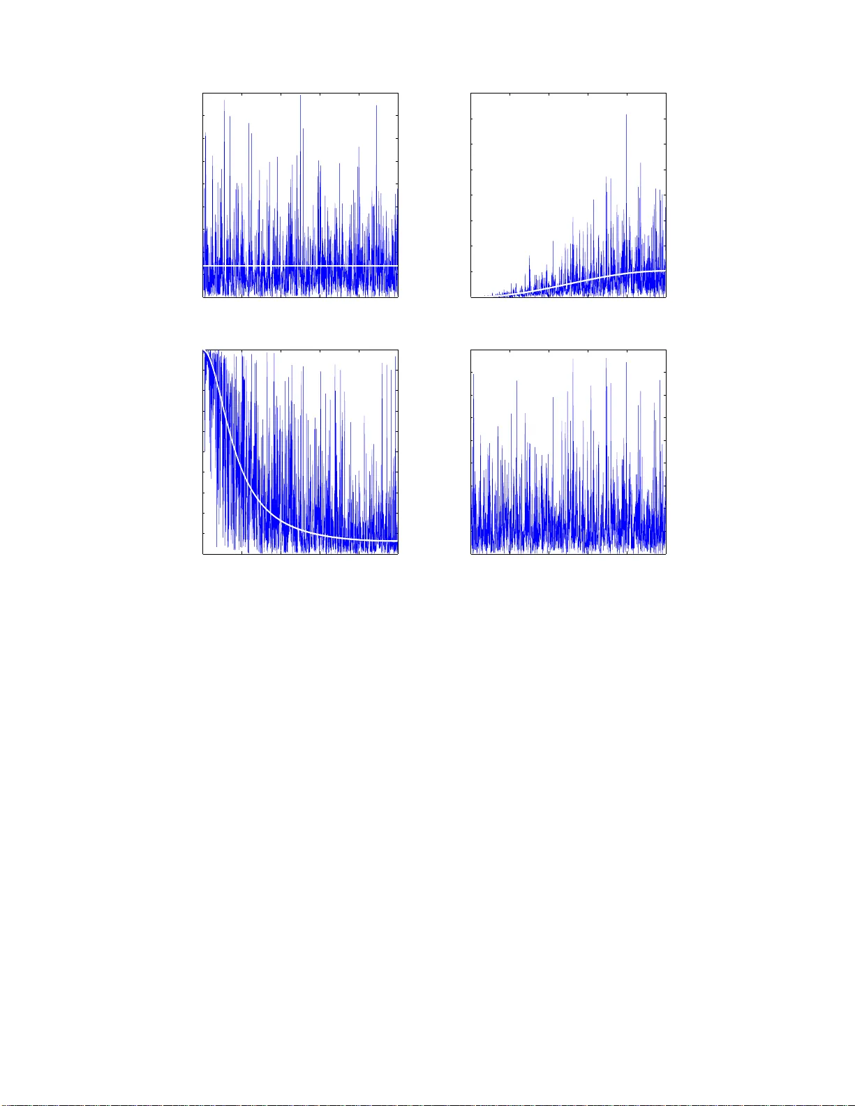
ST A T . SCI. REPOR T 290/ST A TISTICS SECTION REPOR T TR-08-01 1 Multiscale Inference for High-Frequenc y Data Adam Sykulski, Soﬁa C. Olh ede and Grigorios A. Pa vlioti s Abstract This paper pro poses a novel m ultiscale estimator fo r the integrated v olatility o f an It ˆ o process, in the presence of mar ket microstru cture noise (ob servation error). The m ultiscale structu re of the observed process is r epresented frequen cy-by-fr equency and the conce pt of the multiscale ratio is intro duced to quantify the bias in the realized integrated volatility due to th e observation err or . Th e multiscale r atio is estimated fro m a single sample path , and a frequen cy-by-fr equency bias cor rection pro cedure is proposed, which simultan eously reduces variance. W e extend the method to include correlated o bservation erro rs and provide the implied time domain form of the estimatio n proced ure. The ne w method is im plemented to estimate the integrated volatility f or the Heston a nd other models, and the improved pe rforman ce o f our metho d over existing meth ods is illustrated by simu lation studies. Index T erms Bias correction ; market micro structure no ise; r ealized volatility; multiscale inferen ce; Whittle likeliho od. I . I N T RO D U C T I O N Over the las t f ew decades there has been an explosion o f a vailable data in div erse areas such as econ ometrics, atmosphere/oc ean scienc e an d molec ular b iology . It is es sential to use this av ailable data when developing and testing mathe matical mode ls in phy sics, ﬁnanc e, b iology a nd othe r disciplines . It is imperati ve, therefore, to develop accurate and e f ﬁcien t method s for making statistical inferen ce in a p arametric a s well as a non-pa rametric setting. Many interesting p henomen a in the science s are inherently multiscale in the sens e that there is an abundanc e of chara cteristic temporal an d s patial scales . It is q uite often the case that a simpliﬁed, coarse-graine d model is used to describe the es sential features of t he problem under in vestigation. A v a ilable data is then used to estimate parameters in this re duced model [12], [17], [18]. T his renders the problem of s tatistical inference quite s ubtle, since the simpliﬁed models that are be ing u sed a re c ompatible with the data only a t sufﬁciently lar ge scales. In particular , it is not clear how an d if the high frequen cy d ata that is av ailable s hould b e used in the statistical inference proc edure. On the othe r hand in many applications s uch as econ ometrics [32 ] a nd oc eanog raphy [13] the observed data is contaminated b y high frequency observation e rror . Statistical inference for data with a multi sca le structure a nd for da ta contaminated b y high frequ ency noise share c ommon features. In particular the main d if ﬁculty in bo th problems is that the mod el that we wish to ﬁt the data to is not compatible with the data at a ll scales. Th is is an example of a model misspec iﬁcation problem [20, p. 192]. Parametric and non-parame tric estimation for systems with multiple scales and/or the usa ge of high frequen cy data has been s tudied quite extens i vely in the las t few years for the two diff erent types of models. First, the problem of estimating the integrated stochastic volatility in the presence of high frequency observation noise has been co nsidered by various au thors [1], [36]. Similar models and inferenc e problems have also been studied in the context of oceanic transp ort [13]. It was a ssumed in [1], [36] that the obse rved proces s cons ists o f tw o parts, an It ˆ o p rocess X t (i.e. the solution of an SDE, which is a semimartingale) wh ose integrated stoch astic volatil ity (quadratic variation h X t , X t i ) we w ant to estimate, a nd a h igh frequ ency noise compo nent ε t j Y t j = X t j + ε t j . (1) { Y t j } N +1 j =1 are the s ampled obse rvati ons . The additional no ise { ε t j } N +1 j =1 was used to model market microstructure. It was sho wn for the model of (1) that using high frequency da ta leads to a symptotically biased estimators. In particular if all avail able da ta is u sed for the e stimation of the qu adratic variation of X t then the realized inte g rated A. Sykulski and G. A. Pavliotis are with the Department of Mathematics, Imperial College London, South K ensington Campus, SW7 2AZ London, UK (adam.sykulski03@imperial.ac.uk, g.pavliotis@imperial.ac.uk), tel: +44 20 7594 8564, fax +44 20 7594 8517. S. C. Olhede is wi th the Department of S tatistical S cience, Uni versity College London, Gower Str eet, L ondon W C1 E6BT , UK (s.olhede@ucl.ac.uk), t el: +44 20 7679 8321, fax: +44 20 7383 4703. ST A T . SCI. REPOR T 290/ST A TISTICS SECTION REPOR T TR-08-01 2 volatility [ Y t , Y t ] con verges to the a ggregated variance of the differenced obse rvati on noise . Subsa mpling is the refore neces sary for the acc urate estimation of the integrated volatility . An algo rithm for e stimating the integrated volatility which consists of s ubsamp ling at an optimal sa mpling rate co mbined with averaging an d an app ropriate d ebiasing step was propos ed in [1], [36 ]. V arious other estimators were sug gested in [11], [15], [32], [36] for proces ses contaminated by high frequency nuisance s tructure. Second ly , parame ter estimation for fast/slo w sys tems of SDEs for which a limiting S DE for the slow variable can be rigorously shown to exist was s tudied in [24]–[26]. In these papers the problem of making inferences for the parameters of the limiting (coa rse-grained) SDE for the slow variable from obs erved d ata generated by the fast/slo w s ystem w as examined. It w as shown that the maximum likelihood e stimator is asy mptotically bias ed. In order to correctly estimate the parameters in the drift and the diffusion co efﬁcient of the c oarse-grained model from observations of the slow/f ast sys tem using max imum likelihood, subs ampling at an app ropriate rate is ne cess ary . The subsa mpling rate depe nds on the ratio b etween the c haracteristic time scales of the fast a nd slow variables. A similar p roblem, with n o explicit sc ale se paration, was studied in [7]. All o f the pape rs mentioned above propose inference method s in the time doma in. Y et, it would seem natural to an alyse multiscale and high frequency prope rties of the data in the frequency domain. Most of the time do main methods can b e put in a uniﬁed framework as linear ﬁltering techniques , i.e. as a co n volution with a linear kernel, of some time-domain qu adratic function of the da ta. T he understan ding of the se metho ds is enha nced by s tudying them d irectly in the freque ncy domain, as con voluti ons in time are multiplications in frequency . Fourier d omain estimators of the integrated volatility have been p roposed for obse rvati ons devoi d o f microstructure features, se e [2], [14], [21]. Fourier domain estimators have also be en u sed for estimating n oisy It ˆ o p rocesse s (i.e. proces ses of the form 1 ), see [ 22], [29], [30], b ased on smo othing t he time domain quantities by using only a limited numbe r of freque ncies in t he reconstruction. The bias in t he realized integrated volatilit y of the observed proc ess Y t j due to the obs ervation n oise ε t j can be understood directly in the fr eque ncy domain, since the energy as sociated wit h each frequency is contaminated by the microstructure no ise proc ess. This bias is pa rticularly damaging at high frequen cies. In this article we propose a frequency-by-frequency de-biasing procedu re to improve the accu racy of the es timation of the integrated volatilit y . The propos ed estimation me thod can a lso be viewed in the time domain as smoo thing the es timated autoc ov ariance of the increments of the process , but where the implied time domain smoothing kernel is itself estimated from the observed p rocess. In this p aper we will consider a regularly sa mpled It ˆ o process with additi ve wh ite noise ε t j superimpose d upon it a t eac h observation po int t j , cf (1). The It ˆ o proce ss satisﬁes a n SDE of the form dX t = µ t dt + σ t dB t , X 0 = x 0 . (2) B t denotes a standa rd o ne dimensiona l Brownian motion and µ t , σ t are (in gen eral) It ˆ o process es, se e for example the He ston model which is s tudied in Section III. T he Bro wnian motions dri ving the three It ˆ o proc esses c an be correlated. The observations and the process are relate d through Y t j = X t j + ε t j , j = 1 , 2 , . . . , N + 1 , t j := j − 1 N T = ( j − 1)∆ t. (3) W e assume the data is regularly spac ed. The length of the path T is ﬁxed. The additive no ise { ε t j } N +1 j =1 is initially taken to be a white noise proc ess with variance σ 2 ε , and it is as sumed to be indep endent of the noise that driv es the It ˆ o proce ss X t . Our ma in objective is to estimate the integrated volatilit y , h X , X i T = R T 0 σ 2 t dt of the It ˆ o process { X t } , from the se t of o bservations  Y t j  N +1 j =1 . In the ab sence of market micros tructure noise (i.e., when Y t j = X t j , j = 1 , . . . , N + 1 ) the integrated volati lity ca n be estimated from the realized integrated volati lity o f the process { Y t } [32]. In the prese nce of market microstructure noise this is no longer true, see also [36], an d a dif ferent estimation procedu re is necessa ry . The propose d estimator c an be d escribed rough ly as follows. Let { J ( X ) k } den ote the Discrete Fourier Transform (DFT) of the differenced sampled X t process , and similarly for Y t j and ε t j . The integrated volatility can be written in terms of the in verse DFT of the variance of J ( X ) k . W e calculate the bias in the variance of J ( Y ) k , when using its sa mple estimator to estimate the variance o f J ( X ) k . The high frequency c oefﬁcients are he avily con taminated by the micros tructure no ise. W ith a formula for the bias it is possible to debias the e stimated variance of the Fourier transform at every freque ncy , with the unkn own p arameters o f the bias estimated using the Whittle likelihood [34], ST A T . SCI. REPOR T 290/ST A TIST ICS SECTION REPOR T TR-08-01 3 [35]. This produces a de biased estimator of t he integrated v olatility via an a ggregation o f the e stimated v ariance , and we sho w also that the variance of the proposed es timator is reduc ed by the de biasing. Our estimator shows highly compe titi ve mean square error performance; it also has several a dvantages over existing es timators. Fir st, it is robust wi th respec t to the signal to noise ratio; furthermore, it is ea sy to formulate and to implement; in addition, it rea dily genera lizes to the case of correlated observation e rrors (in t ime). Finally , the p roperties of our es timator are tr ans parent us ing frequency domain a nalysis. The rest o f the pap er is organized as follo w s. In Se ction II we introduce o ur estimator and present some of its properties, stated in Th eorems 1 and 2. W e also discuss the time-domain understanding of the prop osed method and the extension of the metho d to the cas e where the observation noise is co rrelated. In Sec tion III we present the results o f Monte Carlo s imulations for our es timator . Section IV is res erved for c onclusion s. V arious technical results are included in the ap pendices . I I . E S T I M AT I O N M E T H O D S Let  Y t j  be given by (3), where the noise  ε t j  is indepe ndent o f  X t j  , is z ero-mean an d its variance at any time is eq ual to σ 2 ε . The s implest estimator of the integrated volatility o f X t would ignore the high fr equ ency compone nt of the data and use the re alized integrated volatil ity of the observed process . The realized integrated volatil ity is giv en by \ h X, X i ( b ) T = [ Y , Y ] T ≡ N X j =1  Y t j +1 − Y t j  2 = O  1 ∆ t  . (4) This es timator is both inc onsistent and biase d, see [15]. For c omparativ e purposes , we de ﬁne also the realized integrated volatil ity of the sa mpled proce ss { X t j } : \ h X, X i ( u ) T = [ X , X ] T ≡ N X j =1  X t j +1 − X t j  2 = O ( N ∆ t ) = O (1) . (5) This canno t b e used in prac tice as X t j is n ot directly o bserved. Both these are es timators o f the integrated volatility (quadratic variation) of X . A. F our ier Domain Pr operties W e shall start by d eri ving an alternati ve representation of (4) to moti vate furt her development. Firstly we deﬁne the increment p rocess of a sa mple from a ge neric time se ries U t j , j = 1 , . . . N + 1 by ∆ U t j = U t j +1 − U t j , j = 1 , . . . N , and then the discrete F ourier Tr ans form of ∆ U t j by J ( U ) k as by [27][p. 206] J ( U ) k = r 1 N N X j =1 ∆ U t j e − 2 π it j f k , f k = k T , U = X , Y , ε. (6) Our propos ed es timator will be b ased on examining the sec ond order properties of { J ( Y ) k } .    J ( Y ) k    2 is the pe ri- odogram [5] d eﬁned for a time se ries and is an inefﬁcient e stimator of v ar { J ( Y ) k } = S ( X ) k ,k . Firstly we examine the properties of { J ( X ) k } . W e hav e, with µ j = 1 ∆ t R j ∆ t ( j − 1)∆ t µ s ds de noting the l oca l average of µ t , ∆ X t j = Z j ∆ t ( j − 1)∆ t [ µ s ds + σ s dW s ] = µ j ∆ t + Z j ∆ t ( j − 1)∆ t σ s dW s , J ( X ) k = r 1 N N X j =1 ∆ X t j e − 2 iπ kj N = r 1 N N X j =1 " ∆ t µ j + Z j ∆ t ( j − 1)∆ t σ s dW s # e − 2 iπ kj N = O  ∆ t 1 / 2 T k  + r 1 N N X j =1 Z j ∆ t ( j − 1)∆ t σ s dW s e − 2 iπ kj N . (7) ST A T . SCI. REPOR T 290/ST A TIST ICS SECTION REPOR T TR-08-01 4 W e de ﬁne ˜ J ( X ) k = r 1 N N X j =1 Z j ∆ t ( j − 1)∆ t σ s dW s e − 2 iπ kj N , and this to leading order approx imates J ( X ) k as ∆ t → 0 for all but a few frequen cies. W e can a lso note that, since µ s is an It ˆ o proc ess, it h as almos t surely continuous paths, which i mplies that ∆ t 2 N − 1 X k =0       r 1 N N X j =1 µ j e − 2 iπ kj N       2 ∼ X k     1 √ N ∆ tN /k     2 = O (∆ t ) (8) ∆ t N − 1 X k =0       r 1 N N X j =1 µ j e − 2 iπ kj N       ∼ X k     1 √ N ∆ tN /k     = O  log(∆ t ) √ ∆ t  , (9) as ∆ t P j µ j e − 2 iπ kj N = O  T k  . So we only ne ed, to leading order , calcu late P N − 1 k =0    ˜ J ( X ) k    2 = O (1) when calculating the p roperties of P N − 1 k =0    J ( X ) k    2 from (8) and (9 ). More formally we note that N − 1 X k =0    J ( X ) k    2 = N − 1 X k =0    ˜ J ( X ) k    2 + O  log(∆ t ) √ ∆ t  . W e need to determine the ﬁrs t and seco nd order structure of { ˜ J ( X ) k } k . In ge neral { ˜ J ( X ) k } k is a co mplex-v alued random v ector , which may n ot be a samp le from a multi variate Ga ussian distribution. Th e c ovari anc e matrix o f a complex random vector Z is given by co v { Z , Z } = E  ZZ H  − E { Z } E { Z } H [23], [28]. W e hav e E n ˜ J ( X ) k o = 0 , k = 1 , . . . , N − 1 . Furthermore, with ˜ S ( X ) k 1 ,k 2 = E n ˜ J ( X ) k 1 ˜ J ( X ) ∗ k 2 o , ˜ S ( X ) k 1 ,k 2 = 1 N E ( N X n =1 Z n ∆ t ( n − 1)∆ t N X l =1 Z l ∆ t ( l − 1)∆ t σ s dW s σ t dW t e − 2 iπ ( k 1 n N − k 2 l N ) ) = 1 N N X n =1 Z n ∆ t ( n − 1)∆ t N X l =1 Z l ∆ t ( l − 1)∆ t E { σ s dW s σ t dW t } e − 2 iπ ( k 1 n N − k 2 l N ) . = 1 N N X n =1 Z n ∆ t ( n − 1)∆ t N X l =1 Z l ∆ t ( l − 1)∆ t E { σ s σ t } δ nl δ ( t − s ) e − 2 iπ ( k 1 n N − k 2 l N ) dsdt. In pa rticular we have that ˜ S ( X ) k ,k = 1 N Z T 0 E  σ 2 s  ds + O  ∆ t 2  := σ 2 X + O  ∆ t 2  = h X, X i T N + O  ∆ t 2  , (10) where the error terms a re due t o the Riemann approximation to an integral and t hus it follo ws t hat N − 1 X k =0 ˜ S ( X ) k ,k = Z T 0 E  σ 2 s  ds + O (∆ t ) . (11) σ 2 X does not depend o n the value of k b ut is con stant irrespectively of the value of k . Mallia vin and Mancino [21] in c ontrast un der very light assump tions show h ow the Fourier coe f ﬁcien ts of { σ 2 t } can be calcula ted from the Fourier co efﬁcients of dX t , using a Parsev al-Rayleigh relationsh ip, see also [22], [30]. W e can from (10) make a stronger link from the Fourier transform to the integrated volatilit y tha n that of the Parseval-Rayleigh relationship, and sh all use t his ‘uniformi ty of ene r gy’ to estimate the mi crostructure bias. ST A T . SCI. REPOR T 290/ST A TIST ICS SECTION REPOR T TR-08-01 5 W e note tha t the c ov ariance betwee n different frequencies is gi ven by: ˜ S ( X ) k 1 ,k 2 = 1 N N X n =1 Z n ∆ t ( n − 1)∆ t E  σ 2 t  dte − 2 iπ n ( k 1 N − k 2 N ) = 1 N Z T 0 E  σ 2 t  dte − 2 iπ t ( k 1 T − k 2 T ) + O  ∆ t 2  . Let Σ ( f ) := R T 0 E σ 2 t e − 2 iπ f t dt . W e can b ound the size of Σ( k 1 T − k 2 T ) as | k 1 − k 2 | increa ses. As E  σ 2 t  is s mooth in t the modulus of t he covariance ca n b e bounded f or increasing | k 1 − k 2 | , as the Fourier tr ans form Σ ( k 1 T − k 2 T ) decays prop ortionally to | k 1 − k 2 | − α − 1 where α is the number of s mooth deriv ativ es of E  σ 2 t  . W e c an also d irectly note that the variance o f the d iscrete Fourier trans form of the no ise is precisely (this is not a large sa mple result) S ( ε ) k 1 ,k 2 = σ 2 ε | 2 sin ( π f k 1 ∆ t ) | 2 δ k 1 ,k 2 , (12) by virtue of being the ﬁrst diff erenc e of white noise (see also [4]). The naive estimator can therefore be re written as, with S ( Y ) k 1 ,k 2 = co v { J ( Y ) k 1 , J ( Y ) k 2 } : \ h X, X i ( b ) T = N X j =1 ∆ Y 2 t j = N − 1 X k =0    J ( Y ) k    2 , (13a) b S ( Y ) k ,k =    J ( Y ) k    2 , (13b) E  \ h X, X i ( u ) T  = N − 1 X k =0 ˜ S ( X ) k ,k + O  log(∆ t ) √ ∆ t  + O (∆ t ) (13c) ≡ N − 1 X k =0 S ( X ) k ,k . (13d) The Parsev al-Rayleigh relations hip in (13a) is discu ssed in [22], and is u sed in [21]. W e s hall now develop a frequency domain s peciﬁca tion of the bias of the naive estimator . Lemma 1: (Frequen cy Domain Bias of the Naive Estimator) Let X t be an It ˆ o proces s and as sume tha t the covari anc e of J ( X ) k 1 and J ( X ) k 2 to be S ( X ) k 1 ,k 2 with the chos en sa mpling. Then the naive estimator of the integrated volatil ity gi ven b y (13) has an expec tation given by: E  \ h X, X i ( b ) T  = N − 1 X k =0  ˜ S ( X ) k ,k + σ 2 ε | 2 sin( π f k ∆ t ) | 2  + O  log(∆ t ) √ ∆ t  (14) = E  \ h X, X i ( u ) T  + N − 1 X k =0 σ 2 ε | 2 sin( π f k ∆ t ) | 2 + O  log(∆ t ) √ ∆ t  = O (1) + O (∆ t − 1 ) + O  log(∆ t ) √ ∆ t  . Pr oof: This resu lt follows from the independenc e of { ε t } a nd { X t } , comb ined with (11) a nd (12). W e notice directly from (14) that the relati ve frequency contribution of ∆ X t and ε t , i.e. S ( X ) k ,k compared to the n oise co ntrib ution σ 2 ε | 2 sin( π f k ∆ t ) | 2 determines the inherent b ias of \ h X, X i ( b ) T . Es timator (13) is incons istent and bias ed since it is equ i valent to estimator (4), and su ch a proc edure would give an unbiase d estimator of the integrated volati lity o nly whe n σ 2 ε = 0 . When the estimator is expresse d in the time do main the microstructure cannot b e disentangled from the It ˆ o proces s. On the other ha nd in the frequency doma in, from the very na ture o f a mu ltiscale proces s, the con trib utions to b S ( Y ) k ,k can be disentangled. ST A T . SCI. REPOR T 290/ST A TIST ICS SECTION REPOR T TR-08-01 6 B. Multiscale Modelling T o correct the b iased estimator we nee d to c orrect the usage of the bias ed e stimator of S ( X ) k ,k , b S ( Y ) k ,k , at eac h frequency . W e therefore deﬁne a new shrinkag e estimator [33, p. 155] of S ( X ) k ,k by b S ( X ) k ,k ( L k ) = L k b S ( Y ) k ,k . (15) 0 ≤ L k ≤ 1 is refe rred to as the multiscale ratio and its optimal form for perfect bias c orrection is for a n arbitrary It ˆ o process giv en by L k = S ( X ) k ,k S ( X ) k ,k + σ 2 ε | 2 sin( π f k ∆ t ) | 2 . (16) This qu antity can not be calculated w ithout exp licit knowledge of S ( X ) k ,k and σ 2 ε . W e c an howev er use (10) to s implify (16) to obtain L k = σ 2 X σ 2 X + σ 2 ε | 2 sin( π f k ∆ t ) | 2 . (17) For a ﬁxed 0 ≤ L k ≤ 1 E n b S ( X ) k k ( L k ) o = L k E     J ( Y ) k    2  = σ 2 X + O ∆ t 3 / 2 k ! , where the order terms follow from the co ntinuity of µ s . W e can deﬁne a new es timator for the true L k via: \ h X, X i ( m 3 ) T = N − 1 X k =0 b S ( X ) k k ( L k ) , where E  \ h X, X i ( m 3 ) T  = h X, X i T + O  log(∆ t ) √ ∆ t  . Recall that h X , X i T = O ( T ) = O (1) . Co nseque ntly , to lead ing order we can remove the bias from the na i ve estimator if we know the multiscale ratio. W e shall no w develop a multiscale understanding o f the p rocess under observation an d use this to cons truct an es timator for the multisca le ratio. C. Estimation of the Mu ltiscale Ratio W e hav e a two-parameter description on how the energy should be adjus ted at each frequency . W e only ne ed to de termine estimators of σ =  σ 2 X , σ 2 ε  . W e propose to implement the estimation us ing the Wh ittle likelihood methods (see [3] or [34], [35]). For a time-domain sample ∆Y = (∆ Y t 1 , . . . , ∆ Y t N ) t hat is stationary , if suitable conditions are satisﬁe d, see for exa mple [8], t hen the Whittle likelihood a pproximates the time doma in likelihood, with improving app roximation as the sample size increas es. It is possible to sh ow a number o f suitable properties of estimators base d on the Whittle likelihood, see [34], [35]. For process es that are not stationary , such cond itions are in ge neral not met, an d so the function can be used as a n objec ti ve function to cons truct estimators, but not as a true li kelihood. The Whittle log -likeli hoo d is deﬁned [34], [35] by l ( S ) ≡ log   N/ 2 − 1 Y k =1 1 S ( Y ) kk e − b S ( Y ) kk S ( Y ) kk   = − N/ 2 − 1 X k =1 log  S ( X ) kk + σ 2 ε | 2 sin( π f k ∆ t ) | 2  − N/ 2 − 1 X k =1 b S ( Y ) kk S ( X ) kk + σ 2 ε | 2 sin( π f k ∆ t ) | 2 . If { ∆ X t } is not stationary , then as long as the total c ontribut ions of the covari anc e of the incremental process can be bounded , using this likelihood will asymptotically (in ∆ t − 1 ) p roduce suitable e stimators, as we sh all disc uss further . ST A T . SCI. REPOR T 290/ST A TIST ICS SECTION REPOR T TR-08-01 7 Deﬁnition 2.1: (Multiscale Energy Likelihood) The multiscale ener gy log-likelihood is then de ﬁned using (10 ) as: l ( σ ) = − N/ 2 − 1 X k =1 log  σ 2 X + σ 2 ε | 2 sin( π f k ∆ t ) | 2  − N/ 2 − 1 X k =1 b S ( Y ) k k σ 2 X + σ 2 ε | 2 sin( π f k ∆ t ) | 2 . (18) W e s tress that strictly sp eaking this may n ot be a (log-)likelihood, but merely a device for determining the mu ltiscale ratio. W e maximise this function in σ to ob tain a se t of estimators b σ . Theorem 1: (The Estimated Multiscale Ra tio) The es timated multiscale ratio is given by b L k = b σ 2 X b σ 2 X + b σ 2 ε | 2 sin( π f k ∆ t ) | 2 , (19) where b σ 2 X and b σ 2 ε maximise ℓ ( σ ) giv en in ( 18) . b L k satisﬁes b L k L k = 1 + O  ∆ t 1 / 4  . (20) Pr oof: See Ap pendix A. Combining (15) with (19) t he proposed estimator of the spec tral density of { ∆ X t } is: b S ( X ) k k ( b L k ) = b L k b S ( Y ) k k , (21) where b L k is giv en by (19). Theorem 2: (The Multiscale Estimator o f the Inte grated V olatility) Assume that ∆ X t j satisﬁes the conditions of Lemma 1 a nd Theorem 1. The multiscale estimator of the integrated volatil ity deﬁned by \ h X, X i ( m 1 ) T = N − 1 X k =0 b S ( X ) k k ( b L k ) , (22) where b S ( X ) k k ( b L k ) is deﬁned by (21) has a mean and v ariance given b y: E  \ h X, X i ( m 1 ) T  = N − 1 X k =0 S ( X ) k k + O  log(∆ t ) √ ∆ t  + O  ∆ t 1 / 4  = Z T 0 E  σ 2 t  + O  log(∆ t ) √ ∆ t  + O  ∆ t 1 / 4  and v ar  \ h X, X i ( m 1 ) T  = N − 1 X k =0 L 2 k    S ( Y ) k ,k    2 + O (∆ t 1 / 2 ) = O (∆ t 1 / 2 ) . Pr oof: See Ap pendix B. W e also n ote that v ar  \ h X, X i ( m 1 ) T  = N − 1 X k =0 L 2 k    S ( Y ) k ,k    2 + O (∆ t 1 / 2 ) < O  1 ∆ t  = v ar  \ h X, X i ( b ) T  , (23) unless σ ε = 0 . W e n ote that the multiscale e stimator has lower variance than the naiv e method of mome nts estimator \ h X, X i ( b ) T due to the fact that 0 ≤ L k ≤ 1 . W e h ave thus removed bia s and simultaneous ly decreas ed the variance, the latter e f fect usually b eing the main purpose of shrinkag e es timators. Note that if we knew the true multiscale ratio L k and used it rather than b L k (i.e. us ed \ h X, X i ( m 3 ) T ) then we would expect an es timator from this quan tity to recover the same variance as the es timator ba sed on the noise -free o bservations. This loss of efﬁciency is inevitable, ST A T . SCI. REPOR T 290/ST A TIST ICS SECTION REPOR T TR-08-01 8 as we have to estimate L k . F inally we can a lso cons truct a Whittle es timator for the integrated volatilit y by starting from (10) and tak ing \ h X, X i ( w ) T = N b σ 2 X . (24) The sampling prope rties of \ h X, X i ( w ) T are found in Ap pendix A, and b σ 2 X is asymp totically unbiased. The results in App endix A imply that v ar  \ h X, X i ( w ) T  = T σ ε τ 1 / 2 X 16 τ 2 X √ ∆ t. (25) W e s ee tha t the variance d epends on the length of the time course, the inv erse of the sign al to noise ratio, the squa re root of the s ampling period and the fourth power of the “a verage standard deviation” of the X t process ., W e may compare the variance of (23) with the variance of (25), to d etermine which e stimator of \ h X, X i ( w ) T and \ h X, X i ( m 1 ) T is prefe rable. W e s hall return to this question of relati ve pe rformance in the examples sec tion, but intuitiv ely argue that \ h X, X i ( w ) T and \ h X, X i ( m 1 ) T are mo re or les s the same estimator , with the latter estimator be ing more intuit ive to explain. D. T ime Domain Understand ing of the Method W e may write the frequency d omain es timator of the s pectral dens ity of ∆ X t in the time domain to clarify s ome of its properties. W e deﬁne b s ( X ) τ = 1 N N − 1 X k =0 b S ( X ) k k e 2 iπ kτ N , τ ∈ N , which when ∆ X t is a stationary p rocess corresponds to the estimated autocovari anc e seque nce of ∆ X t using the method of moments estimator [5, Ch. 5]. W e then ha ve b S ( X ) k k = L k b S ( Y ) k k , b s ( X ) τ = X u ℓ τ − u b s ( Y ) u , (26) and s o the estimated autoc ov ariance of the ∆ X t process , namely b s ( X ) τ , is a s moothed version of b s ( Y ) τ . W e can therefore view b S ( X ) k k as the Fourier transform of a s moothed version of the a utocovariance seq uence of ∆ Y t . W e let L ( f ) = σ 2 X σ 2 X + σ 2 ε | 2 sin( π f ∆ t ) | 2 , ( 27) be the continuous analog ue of L k . T o ﬁnd the smo othing kernel we are using we need to calculate ℓ τ = 1 N N − 1 X k =0 L k e 2 iπ kτ N = Z 1 2 − 1 2 σ 2 X σ 2 X + 4 σ 2 ε sin 2 ( π f ) e 2 iπ f τ d f + O (∆ t ) . (28) Thus u tilizing integration in the complex p lane (see Appendix C) we obtain that ℓ τ =       σ 2 ε σ 2 X  τ + O   σ ε σ X  2 τ +2  if σ 2 ε < σ 2 X σ X 2 σ ε  1 − σ X σ ε  τ + O  σ 2 X 2 σ 2 ε  1 − σ X σ ε  τ  if σ 2 ε > σ 2 X (29) These a re both decreas ing se quenc es in τ . W e write r τ = σ X 2 σ ε  1 − σ X σ ε  τ . If we can additionally a ssume that L ( f ) decreas es s uf ﬁcien tly rapidly to be ne ar zero by f = 1 π then we ﬁnd that ℓ τ ≈ q τ = σ X 2 σ ε e − σ X σ ε | τ | . ST A T . SCI. REPOR T 290/ST A TIST ICS SECTION REPOR T TR-08-01 9 −25 −20 −15 −10 −5 0 5 10 15 20 25 0 0.01 0.02 0.03 0.04 0.05 0.06 0.07 0.08 0.09 lag, τ l τ r τ q τ φ τ −40 −30 −20 −10 0 10 20 30 40 −0.01 0 0.01 0.02 0.03 0.04 0.05 0.06 0.07 0.08 0.09 lag, τ Fig. 1. ℓ τ as well as r τ and q τ for a chosen valu e of the S NR (left). The approximate weighting fun ctions perfectly mirror the exact calculation. W e overlay a Gaussian kernel with the same spread for comparison. ℓ τ estimated for the MA(6) case (right). In the limit of no obs ervation noise ( σ X σ ε → ∞ ) then this s equen ce becomes a delta function ce ntered at τ = 0 . Let us plot these functions, i.e. ℓ τ , r τ and q τ for a chosen case of σ 2 X /σ 2 ε ≈ 0 . 0331 (the approximate SNR used in a later example), in Figure 1 (left). W e se e that theo ry coincides very well with prac tise, and almos t perfect agreement betwee n the three functions. ℓ τ is howev er a strange choice of kerne l, if dictated by the statistical inference p roblem: it h as heavier tails than the common choice of the Gaussian kernel, and is extremely peaked around zero (a Gauss ian kernel with the same variance has bee n overlaid in F igure 1). This is no t s trange, a s we a re trying to ﬁlter out c orrelations du e to non-It ˆ o behaviour , but c ounter to our intuition abou t s uitable kernel functions , as the d if ferenced It ˆ o proces s exhibits very little covariance at any lag but zero, the s harp pe ak at zero is n ecess ary . E. Correlated Er r ors In many applications we need to cons ider correlated ob servation noise . W e assume that despite being d epende nt the ε t j is a stationary time series. Stationa ry proc esses can be con veniently represented in terms of aggregations of un correlated white noise proces ses, us ing the W old dec omposition theorem [6][p. 187 ]. W e may therefore write the z ero-mean obse rvati on ε t j as ε t j = ∞ X k =0 θ t k η t j − t k , (30 ) where θ t 0 ≡ 1 , P j θ 2 t j < ∞ , and { η t n } sa tisﬁes E { η t n } = 0 and E { η t n η t m } = σ 2 η δ n,m , a mo del also used in [31]. Common practise would in volve approximating the variable by a ﬁnite number of elements in the sum, and thus we truncate (30) to s ome q ∈ Z . W e therefore model the n oise as a Moving A verage (MA) process speciﬁed by ε t j = η t j + q X k =1 θ t k η t j − k , (31) and the cov ariance o f the DFT of the dif ferenced ε t j process takes the form: S ( ε ) k ,k = σ 2 η      1 + q X k =1 θ k e 2 iπ f k      2 | 2 sin ( π f ∆ t ) | 2 . (32) This leads t o deﬁning a new multiscale ratio replacing σ 2 ε | 2 sin ( π f ∆ t ) | 2 of ( 17) with σ 2 η   1 + P q k =1 θ k e 2 iπ f k   2 | 2 sin ( π f ∆ t ) | 2 . W e then obtain a new e stimator of S ( X ) k k . In general the value of q is not known. T o s imultaneously implement model ch oice, we need to penalize the likelihood. W e de ﬁne the corrected Aika ke information criterion (AICC) by [6, p. 3 03] (refer to (18) for l ( σ , θ ) with σ 2 ε | 2 sin ( π f ∆ t ) | 2 replaced by σ 2 η   1 + P q k =1 θ k e 2 iπ f k   2 | 2 sin ( π f ∆ t ) | 2 ) AICC( θ ) = − 2 l ( σ , θ ) + 2 ( p + 2) n n − p − 3 . (33) ST A T . SCI. REPOR T 290/ST A TIST ICS SECTION REPOR T TR-08-01 10 By minimizing this func tion, in σ , θ and q , we obta in the b est ﬁtting mo del for the n oise acco unting for overﬁtting by using the penalty term. W ith this method we retrie ve a new multiplier that is applied in the Fourier do main, which c orresponds to a new smoothe r in the Fourier domain, where the s moothing wind ow (and its smoothing width) h ave b een a utomatically chosen by the data. See an example of such a smoothing window ℓ τ in in Figure 1 (right). Here L k has b een estimated from an It ˆ o process immerse d in an MA nois e proce ss. The spectrum of the MA has a trough at freque ncy 0.42. W e the refore expe ct to reinforce osc illations a t period 1 / 0 . 42 ≈ 2 . 5 , which is evident from the oscillations o f the e stimated kernel. For more de tails of this process s ee section III-E. I I I . M O N T E C A R L O S T U D I E S In this s ection we demons trate the performance of the mu ltiscale estimator through Monte Carlo simulations. W e ﬁrst d escribe the de-biasing proce dure o f the es timator for the Heston Model using Fourier do main graphs. W e then present bias, variance and mea n s quare e rror results of various estimators (including the mu ltiscale e stimator , the n aiv e e stimator a nd the ﬁrst-best estimator developed in [36]), for the Heston Mod el a s well as Brownian and Ornstein Uhlenbe ck process es. W e then co nsider t he case wh ere the sample path in a Hes ton Mod el is much shorter and another case where the microstructure noise is greatly reduced. Finally , we consider the case o f correlated errors a nd show how a stationary noise proce ss ca n be c aptured us ing mode l c hoice metho ds a nd then the integrated volatil ity can be e stimated using the a djusted multisca le estimator . A. The Heston Model The Hes ton mode l is sp eciﬁed in [16]: dX t = ( µ − ν t / 2) dt + σ t dB t , dν t = κ ( α − ν t ) dt + γ ν 1 / 2 t dW t , (34) where ν t = σ 2 t , and B t and W t are correlated 1-D Bro wnian motions. W e will use the same parameter v alues to the ones tha t were used in [36], namely µ = . 05 , κ = 5 , α = . 04 , γ = . 5 and the correlation coef ﬁcient between the two Bro wnian motions B and W is ρ = − . 5 . W e se t X 0 = 0 and ν 0 = 0 . 04 , which is the long time limit of the expe ctation of the proces s ν t . 1 W e calcula te b S ( X ) k k and b S ( ε ) k k directly from simulated data and average acros s realizations , prod ucing Figu re 2, where k is indicated by its freque ncy f k = k / N , a nd only plotted for k = 0 , . . . , N / 2 − 1 , as the sp ectrum (or S ( X ) k k ) is symmetric. W e see directly from thes e p lots that (on average as we sh owed) b S ( X ) k k is c onstant whilst b S ( ε ) k k is strongly increasing with k , c ompletely d warﬁng the other spec trum at large k . (11) implies that an equa l we ighting is given to all frequenc ies for the dif ferenced It ˆ o process. The noise proces s will in contrast ha ve a spectrum that is far from ﬂat, and a suitable bias correction would shrink t he estimator of S ( X ) k k at high er frequencie s. W e also ca lculate b S ( X ) k k and b S ( ε ) k k for one simulated path, d isplayed in Figure 3. Here we have used the sa me sample length T and n oise intensity σ 2 ε as in [36]: T = 1 da y a nd σ 2 ε = 0 . 0005 2 . Th e length of the sample path, T = 1 day or 23 , 400 s with ∆ t = 1 s , correspo nds to one trading day , since we take one trading day to be 6 . 5 h long. No tice the dif ferent shape of the two periodograms. b S ( Y ) k k will not be d istinguishable from b S ( ε ) k k at higher frequencies, de spite the moderate to low intensity of the market microstructure noise. If we obse rved the two components X t and ε t separately , then t he multiscale ratio L k could be e stimated from b S ( X ) k k and b S ( ε ) k k using the me thod of moments formula. In this c ase, we would es timate L k by the sample Fourier T rans form variances e L k = b S ( X ) k k b S ( X ) k k + b S ( ε ) k k . (35) The co rresponding estimator o f the integr ated v olatility be comes \ h X, X i ( m 2 ) T = N − 1 X k =0 e L k b S ( Y ) k k . (36) The es timated multiscale ratio e L k , for the Heston model with the spec iﬁed parameters, is plotted in Figure 4. 1 lim t → + ∞ E ν t = α. ST A T . SCI. REPOR T 290/ST A TIST ICS SECTION REPOR T TR-08-01 11 0 0.1 0.2 0.3 0.4 0.5 0 1 2 3 4 5 6 7 8 x 10 −8 frequency 0 0.1 0.2 0.3 0.4 0.5 0 1 2 3 4 5 6 7 8 9 x 10 −6 frequency Fig. 2. b S ( X ) kk (left) and b S ( ε ) kk (right) averaged over 100,000 realizations. Note the different scaling of the y axis in t he two ﬁgures. 0 0.1 0.2 0.3 0.4 0.5 0 1 2 3 4 5 6 7 8 x 10 −8 frequency 0 0.1 0.2 0.3 0.4 0.5 0 1 2 3 4 5 6 7 8 9 x 10 −6 frequency 0 0.1 0.2 0.3 0.4 0.5 0 1 2 3 4 5 6 7 8 x 10 −8 frequency 0 0.1 0.2 0.3 0.4 0.5 0 1 2 3 4 5 6 7 8 x 10 −8 frequency Fig. 3. A realisation of b S ( X ) kk (top left), a realisation of b S ( ε ) kk (top right) wi th the Whittle estimates superimpose d and of t wo biased corrected estimators of S ( X ) kk , using e L k b S ( X ) kk (bottom left) and b L k b S ( Y ) kk (bottom right). Notice the differen t scales in the four ﬁgures. E stimated spectra are plotted on a li near scale for ease of comparison to t he effect of applying b L k . ST A T . SCI. REPOR T 290/ST A TIST ICS SECTION REPOR T TR-08-01 12 0 0.1 0.2 0.3 0.4 0.5 0 0.1 0.2 0.3 0.4 0.5 0.6 0.7 0.8 0.9 1 frequency Fig. 4. The method of moments estimate e L k from a single realisation, with the W hittle estimate (white line) of L k superimposed. The multiscale ratio cannot be estimated using the method of moments in realistic sce narios, as we only obse rve the ag gregated process Y t and not the two proc esses X t and ε t separately . Figu re 3 displays the es timated multiscale ratio e L k applied to b S ( Y ) k k over one path rea lisation. This plot s uggests that the ene r gy over the high frequenc ies has been s hrunk and that e L k b S ( Y ) k k is a go od app roximation to b S ( X ) k k . It therefore seems not un reasona ble that the summation of this function ac ross frequenc ies should ma ke a goo d app roximation to the integrated volatility . The pa rameters ( b σ 2 X and b σ 2 ε ) are fou nd se parately for each pa th using t he MA TLAB function fmincon on (18). Figure 3 shows b σ 2 X and b σ 2 ε | 2 sin ( π f k ∆ t ) | 2 (in white) plotted over the pe riodograms b S ( X ) k k and b S ( ε ) k k for one s imulated path. The approximated v alues of σ 2 X and σ 2 ε are quite similar to the a veraged periodograms of Figu re 2; in fact the accuracy o f the new estimator depends on how cons istently thes e parame ters a re estimated in the pres ence of limited information from the s ampled proces s Y t . Figu re 4 sho ws the co rresponding es timated multiscale ratio b L k (in white) from this simulated path, as deﬁne d in (19). The fun ction dec ays, as exp ected, so tha t it will remove the high-frequency micros tructure noise i n the s pectrum of Y t ; the ratio is also a good a pproximation of e L k . Figure 3 shows b L k b S ( Y ) k k , which is again similar to b S ( X ) k k . It would appear that the new estimator has successfully remov ed the micros tructure effect from eac h frequency . It is worth no ting tha t the ratios L k and b L k quantify the effect of the multiscale structure of the proces s. If σ 2 ε is zero (ie. there is no microstructure no ise), then no correction will be made to the spec tral density function (the rati o will equal 1 at all frequencies ). So in the case of zero microstructure noise, the es timate w ould recover b S ( X ) k k and from (13) the estimate of the integrated volatil ity would s imply be the realized integrated volatil ity of the o bservable proces s. W e in vestigate the performance of the multisca le estimator using Mon te Ca rlo simulations. In this study 50, 000 simulated paths are ge nerated. T able I disp lays the results of ou r simulation, where biase s, variances and errors are calculated using a Riemann su m approximation of the integral T N N X i =1 σ 2 i = Z T 0 σ 2 t dt. (37) The two es timators \ h X, X i ( u ) T and \ h X, X i ( m 2 ) T (see (5) and (36) respectively) are both included for comparison, ev en thoug h these req uire us e of the unobs ervable X t process . The performance of the ﬁrst-best es timator in [ 36] (denoted by \ h X, X i ( s 1 ) T ) is also included as a we ll-performing an d tested e stimator us ing only the Y t process , as is the nai ve e stimator of the realize d volatility on Y t at the highest frequ ency , \ h X, X i ( b ) T , gi ven in (4) (the ﬁfth-best ST A T . SCI. REPOR T 290/ST A TIST ICS SECTION REPOR T TR-08-01 13 Sample bias Sample variance Sample RMSE \ h X, X i ( b ) T 1 . 17 × 10 − 2 1 . 80 × 10 − 8 1 . 17 × 10 − 2 \ h X, X i ( s 1 ) T 6 . 44 × 10 − 7 2 . 76 × 10 − 10 1 . 66 × 10 − 5 \ h X, X i ( m 1 ) T 2 . 90 × 10 − 7 2 . 59 × 10 − 10 1 . 61 × 10 − 5 \ h X, X i ( w ) T 2 . 63 × 10 − 7 2 . 59 × 10 − 10 1 . 61 × 10 − 5 \ h X, X i ( m 2 ) T 1 . 39 × 10 − 8 2 . 07 × 10 − 10 1 . 44 × 10 − 5 \ h X, X i ( u ) T 1 . 20 × 10 − 8 2 . 06 × 10 − 10 1 . 44 × 10 − 5 T ABLE I S I M U L A T I O N S T U DY C O M P A R I N G T H E N E W E S T I M AT O R W I T H T H E B E S T E S T I M A T O R O F [ 3 6 ] . −4 −3 −2 −1 0 1 2 3 4 x 10 −5 0 500 1000 1500 2000 2500 3000 3500 4000 −4 −3 −2 −1 0 1 2 3 4 5 x 10 −5 0 500 1000 1500 2000 2500 3000 3500 4000 Fig. 5. The histograms of the observed bias of the proposed estimator (a), and the ﬁrst-best estimator (b), ov er 100,000 sample paths. estimator in [36]). W e also inc lude the performance of \ h X, X i ( w ) T , de ﬁned in (24 ). T able I shows that the n ew e stimator , \ h X, X i ( m 1 ) T , is c ompetiti ve with the ﬁrst-best approa ch in [36], \ h X, X i ( s 1 ) T , as an es timator of the integrated volatility for the Heston model with the stated parame ters. For this s imulation the new method performed marginally better . T he similar performance of the tw o estimators is quite remarkable, giv en their different approach ; both estimators in volve a bias-correction, [36] pe rform this globa lly by weigh ting dif ferent sa mpling frequ encies, whilst we co rrect loca lly at eac h frequen cy . The realized integrated volatil ity o f Y t at the highest frequency , \ h X, X i ( b ) T , prod uces disastrous results, a s expecte d. W e also n ote that \ h X, X i ( m 1 ) T performs more or less identically to \ h X, X i ( w ) T . The se two estimators can a lmost be us ed interc hangea bly d ue to the in variance prope rty of a maximum likelihood e stimator . This o bservation is born out by our simulation studies, and we hen ceforth only report results for \ h X, X i ( m 1 ) T . Note that the variance of \ h X, X i ( w ) T can be found from (25 ). T o co mpare theory with simulations we note that the average es timated standard deviation is 1 . 6093 × 10 − 5 whilst the express ion for the variance to lea ding orde r gives an expression for the standard deviation of  v ar  \ h X, X i ( w ) T  1 / 2 = 1 . 0246 × 10 − 5 , u sing the p arameter values of σ 2 X ≈ 6 . 8 × 10 − 9 and σ 2 ε ≈ 2 . 5 × 10 − 7 . A histogram of the ob served bias of the new e stimator is plotted in Figure 5 along with a histog ram o f the observed bias of the ﬁrst-best e stimator in [36]. Th e observed bias of our estimator follows a Gau ssian distrib ution centred at zero, sug gesting that this estimator is unb iased, as ou t results cla im to be true. Co mparing our estimator to the ﬁrst-best estimator , it can be seen that the new estimator has similar magnitudes of error also (henc e the similar Ro ot Mean S quare Error (RMSE)) . ST A T . SCI. REPOR T 290/ST A TIST ICS SECTION REPOR T TR-08-01 14 4 5 6 7 8 9 10 11 x 10 −9 0 500 1000 1500 2000 2500 3000 3500 4000 2.35 2.4 2.45 2.5 2.55 2.6 2.65 2.7 x 10 −7 0 500 1000 1500 2000 2500 3000 3500 4000 Fig. 6. The histograms of the estimated σ 2 X (a) and σ 2 ε (b). Sample bias Sample variance Sample RMSE \ h X, X i ( b ) T 1 . 17 × 10 − 2 1 . 77 × 10 − 8 1 . 17 × 10 − 2 \ h X, X i ( s 1 ) T 6 . 52 × 10 − 7 2 . 68 × 10 − 11 5 . 22 × 10 − 6 \ h X, X i ( m 1 ) T 3 . 02 × 10 − 7 1 . 98 × 10 − 11 4 . 46 × 10 − 6 \ h X, X i ( m 2 ) T 1 . 96 × 10 − 9 6 . 93 × 10 − 13 8 . 32 × 10 − 7 \ h X, X i ( u ) T 3 . 79 × 10 − 9 5 . 44 × 10 − 13 7 . 38 × 10 − 7 T ABLE II S I M U L A T I O N S T U DY F O R T H E B R O W N I A N P RO C E S S . The new e stimator requ ires c alculation of b σ 2 X and b σ 2 ε which will vary over ea ch proces s due to the limited information giv en from the Y t process . The stab ility of this estimation is of great importance if t he estimator is to perform well. Figure 6 shows the distrib ution of the p arameters b σ 2 X and b σ 2 ε over the simulated paths. Th e parameter estimation is quite c onsistent, with all values e stimated within a na rro w range . Figure 2 sugges ts that the se estimates are roughly unbiased; as σ 2 X ≈ 6 . 8 × 10 − 9 and σ 2 ε ≈ 2 . 5 × 10 − 7 (as σ 2 ε | 2 sin ( π f k ) | 2 ≈ 1 × 10 − 6 , at f k = 0 . 5 ). B. Br ownian Process and Ornstein Uhlenbeck Pr ocess W e repeated ou r simulations for a Bro wnian Process g i ven by: dX t = q 2 σ 2 t dB t , (38) where σ 2 t = 0 . 01 . W e o therwise keep t he same simulation setup as before with 50,000 simulated paths of length 23,400. The res ults are display ed in T able II . The n ew e stimator , \ h X, X i ( m 1 ) T , aga in delivers a marked improvement on the nai ve estimator , \ h X, X i ( b ) T , an d performs ma r ginally better than the ﬁrst-bes t es timator in [36 ], \ h X, X i ( s 1 ) T . W e also p erformed a Monte Ca rlo simulation for the Orns tein Uhlenbe ck proces s given by : dX t = X t dt + √ 2 σ t dB t , (39) where also σ 2 t = 0 . 01 . Again we retain the same simulation setup and the results are displayed in T ab le II I . The results are almost identical to that of the Bro wnian process , with the new estimator aga in outperforming other time-domain e stimators. ST A T . SCI. REPOR T 290/ST A TIST ICS SECTION REPOR T TR-08-01 15 Sample bias Sample variance Sample RMSE \ h X, X i ( b ) T 1 . 17 × 10 − 2 1 . 78 × 10 − 8 1 . 17 × 10 − 2 \ h X, X i ( s 1 ) T 6 . 69 × 10 − 7 2 . 66 × 10 − 11 5 . 20 × 10 − 6 \ h X, X i ( m 1 ) T 2 . 95 × 10 − 7 1 . 97 × 10 − 11 4 . 44 × 10 − 6 \ h X, X i ( m 2 ) T 5 . 09 × 10 − 9 6 . 76 × 10 − 13 8 . 22 × 10 − 7 \ h X, X i ( u ) T 6 . 29 × 10 − 9 5 . 33 × 10 − 13 7 . 30 × 10 − 7 T ABLE III S I M U L A T I O N S T U D Y F O R T H E O R N S T E I N U H L E N B E C K P R O C E S S . Sample bias Sample variance Sample RMSE \ h X, X i ( b ) T 1 . 17 × 10 − 3 2 . 29 × 10 − 9 1 . 17 × 10 − 3 \ h X, X i ( s 1 ) T 1 . 00 × 10 − 6 4 . 51 × 10 − 10 2 . 13 × 10 − 5 \ h X, X i ( m 1 ) T 1 . 84 × 10 − 7 4 . 23 × 10 − 10 2 . 06 × 10 − 5 \ h X, X i ( m 2 ) T 4 . 80 × 10 − 8 2 . 42 × 10 − 10 1 . 55 × 10 − 5 \ h X, X i ( u ) T 5 . 27 × 10 − 8 2 . 28 × 10 − 10 1 . 51 × 10 − 5 T ABLE IV S I M U L A T I O N S T U DY F O R S H O RT E R S A M P L E R L E N G T H . C. Compar ing estimators over sho rter sample lengths This s ection c ompares e stimators for a s horter sa mple length which will reduce the beneﬁt of subsampling due to the v ariance iss ues of small-l ength data but will also affect the variance of the multiscale rati o ( cf Theo rem 1). The simulation setup is exactly the same a s before (using the Heston model wit h the s ame parameters) except that T , the simulation length, is reduced by a factor of 10 to 0.1 d ays or 2340 s . Before the results o f the s imulation are reported, it is of interes t to see whether the frequency do main method s developed still model each process accurately . Figure 7 sh ows the c alculated b σ 2 X and b σ 2 ε | sin( π ∆ tf k ) | 2 (in white) toge ther with the periodo grams b S ( X ) k k and b S ( ε ) k k for one simulated path. The estimator stil l approximates the energy structure of the p rocesse s ac curately . Figure 7 also shows the corresp onding estimate of the multiscale ratio b L k (in white) from this simulated pa th (together with e L k ) and the corresp onding plot of b L k b S ( Y ) k k . The new e stimator h as removed the microstructure noise eff ect and ha s formed a g ood a pproximation of b S ( X ) k k . The approximation o f the periodog rams is still ac curate despite the shortening of available data. T able IV d isplays the ac curacy o f the e stimators over the 50,000 simulated pa ths. The ﬁrst-best es timator in [36], \ h X, X i ( s 1 ) T , an d the n ew es timator , \ h X, X i ( m 1 ) T , are once again comparable in performance and b oth estimates are close to the best attainab le RMSE gi ven by , \ h X, X i ( u ) T , the realized integrated volatil ity on X t . D. Compar ing estimators with a low-noise process This section compares e stimators for smaller le vels of mi crostructure noise. Reducing the microstructure noise will reduce the nee d to subsample. The ﬁrst-best estimator in [36], \ h X, X i ( s 1 ) T , will have a higher samp ling freque ncy and the new estimator will reduc e its es timate of b σ 2 ε accordingly . For very sma ll lev els of noise, howev er , the ﬁrst-best e stimator will bec ome zero, a s the op timal numbe r of samples bec omes n (the h ighest avail able). This possibility is now examine d, us ing the Heston model a s before, with all parameters unch anged exce pt the no ise is reduced by a factor o f 10, ie. σ 2 ε = 0 . 00005 2 . Note that the path length is kept at its original length of T = 1 day . Figure 8 shows the e stimates of b σ 2 X and b σ 2 ε | 2 sin ( π ∆ tf k ) | 2 (in w hite) a long with the pe riodograms b S ( Y ) k k and b S ( ε ) k k for o ne simulated path along with the corresponding e stimate of the multiscale ratio b L k (in w hite) (plotted over the approximated e L k ) and the c orresponding plot of b L k b S ( Y ) k k . The es timation metho d works well again; notice how the mag nitude of the microstructure noise has be en greatly reduced (the sca le is now of order 10 − 8 rather than 10 − 6 ) ca using the multiscale ratio L k to b e more tempered across the high frequenc ies than it was b efore, due ST A T . SCI. REPOR T 290/ST A TIST ICS SECTION REPOR T TR-08-01 16 0 0.1 0.2 0.3 0.4 0.5 0 0.5 1 1.5 2 2.5 3 3.5 4 4.5 x 10 −7 frequency 0 0.1 0.2 0.3 0.4 0.5 0 1 2 3 4 5 6 7 8 x 10 −6 frequency 0 0.1 0.2 0.3 0.4 0.5 0 0.1 0.2 0.3 0.4 0.5 0.6 0.7 0.8 0.9 1 frequency 0 0.1 0.2 0.3 0.4 0.5 0 0.5 1 1.5 2 2.5 3 3.5 4 4.5 x 10 −7 frequency Fig. 7. A realisation of b S ( X ) kk (top left), a realisation of b S ( ε ) kk (top right) wi th the W hittle estimates superimposed, t he estimate of L k (bottom left) with the W hittle estimate of L k superimposed and the biased corrected estimator of S ( X ) kk using b L k b S ( Y ) kk (bottom right). Notice the differe nt scales in the four ﬁgures. to the smaller micros tructure noise. Nonethe less, the new estimator has still detecte d the smaller levels of no ise in the d ata. T able V re ports on the resu lts o f 50,000 simulations pe rformed as before. The ﬁrst-bes t e stimator of [36], \ h X, X i ( s 1 ) T , c ategorically failed for this mo del. This is du e to the fact that the optimal numbe r of samples was always e qual to n , the total number of samples av ailable. The refore, the ﬁrst-best e stimator was always ze ro. The second -best estimator in [36], d enoted by \ h X, X i ( s 2 ) T , was reas onably ef fective. This is simply an e stimator that av erage s es timates calculated from sub -sampled p aths at diff erent starting points a nd is therefore asy mptotically biased. The new estimator , \ h X, X i ( m 1 ) T , was remarkably robust, with RMSE very close to the RMSE of estimators based on the X t process . Th e difference in performance between estimators u sing Y t and estimators us ing X t is expected to become smaller with less microstructure noise and this can be se en by the similar order RMSE e rrors between all es timators. Nevertheless, the new e stimator was much clos er in performance to the realized integrated volatil ity o n X t than it was to any other estimator on Y t , a result that demons trates the precision and rob ustnes s of this ne w es timator of int egrated volatilit y . E. Correlated No ise In this section we consider microstructure n oise that is correlated. If this proce ss is stationa ry , the noise process can be mode lled as a n MA process (as d escribed in Se ction II-E), and the c orresponding parameters can be es timated by maximising the multiscale Wh ittle likelihood using (17) and (32). Figure 9 shows the multiscale e stimator ST A T . SCI. REPOR T 290/ST A TIST ICS SECTION REPOR T TR-08-01 17 0 0.1 0.2 0.3 0.4 0.5 0 1 2 3 4 5 6 7 x 10 −8 frequency 0 0.1 0.2 0.3 0.4 0.5 0 1 2 3 4 5 6 7 8 x 10 −8 frequency 0 0.1 0.2 0.3 0.4 0.5 0 0.1 0.2 0.3 0.4 0.5 0.6 0.7 0.8 0.9 1 frequency 0 0.1 0.2 0.3 0.4 0.5 0 1 2 3 4 5 6 7 x 10 −8 frequency Fig. 8. A realisation of b S ( X ) kk (top left), a realisation of b S ( ε ) kk (top right) wi th the W hittle estimates superimposed, t he estimate of L k (bottom left) with the W hittle estimate of L k superimposed and the biased corrected estimator of S ( X ) kk using b L k b S ( Y ) kk (bottom right). Notice the differe nt scales in the four ﬁgures. Sample bias Sample variance Sample RMSE \ h X, X i ( b ) T 1 . 17 × 10 − 4 2 . 11 × 10 − 10 1 . 18 × 10 − 4 \ h X, X i ( s 2 ) T 3 . 53 × 10 − 6 1 . 00 × 10 − 9 3 . 19 × 10 − 5 \ h X, X i ( m 1 ) T 7 . 63 × 10 − 9 2 . 12 × 10 − 10 1 . 46 × 10 − 5 \ h X, X i ( m 2 ) T 7 . 91 × 10 − 9 2 . 06 × 10 − 10 1 . 44 × 10 − 5 \ h X, X i ( u ) T 9 . 83 × 10 − 9 2 . 05 × 10 − 10 1 . 43 × 10 − 5 T ABLE V S I M U L A T I O N S T U DY F O R L OW E R M A R K E T M I C R O S T R U C T U R E N O I S E . applied to the Hes ton Model (with the same parame ters as be fore) with a micros tructure n oise that follows an MA(6) p rocess ( parame ters given in the c aption). The Whittle estimates (in white) form a g ood approximation of b S ( X ) k k and b S ( ε ) k k despite the more complicated n uisance s tructure. The correspon ding es timate of the mu ltiscale ratio b L k (in w hite) therefore removes energy from the correct frequenc ies an d the corresp onding p lot of b L k b S ( Y ) k k is a good approximation of b S ( X ) k k . This is the same noise process and It ˆ o process for which we calculated the op timal smoothing window in sec tion II-E, an d the troug h in the no ise at abou t f = 0 . 42 c orresponds to the oscillations in the kernel plott ed i n Figure 1. If the length of the MA ( p ) p rocess is unkn own, then p c an be determined using (33). In T ab le VI we s how an ST A T . SCI. REPOR T 290/ST A TIST ICS SECTION REPOR T TR-08-01 18 0 0.1 0.2 0.3 0.4 0.5 0 1 2 3 4 5 6 7 x 10 −8 frequency 0 0.1 0.2 0.3 0.4 0.5 0 1 2 3 4 5 6 7 8 9 x 10 −6 frequency 0 0.1 0.2 0.3 0.4 0.5 0 0.1 0.2 0.3 0.4 0.5 0.6 0.7 0.8 0.9 1 frequency 0 0.1 0.2 0.3 0.4 0.5 0 1 2 3 4 5 6 7 x 10 −8 frequency Fig. 9. A realisation of b S ( X ) kk (top left), a realisation of b S ( ε ) kk (top right) wi th the W hittle estimates superimposed, t he estimate of L k (bottom left) wit h the Whittle estimate of L k superimposed and the biased corrected estimator of S ( X ) kk using b L k b S ( Y ) kk (bottom right). In this example we use an MA(6) with θ 1 = 0 . 5 , θ 2 = − 0 . 1 , θ 3 = − 0 . 1 , θ 4 = 0 . 2 , θ 5 = 0 and θ 6 = 0 . 4 . Notice the different scales in the four ﬁgures. MA( p ) θ 1 θ 2 θ 3 θ 4 θ 5 θ 6 θ 7 θ 8 AICC p = 1 0.935 − 3 . 208490 × 10 5 p = 2 0.624 -0.445 − 3 . 239947 × 10 5 p = 3 0.658 -0.459 -0.046 − 3 . 240000 × 10 5 p = 4 0.806 -0.603 -0.101 0.410 − 3 . 262427 × 10 5 p = 5 0.813 -0.606 -0.101 0.411 -0.008 − 3 . 262416 × 10 5 p = 6 0.815 -0.604 -0.097 0.420 -0.003 0.000 − 3 . 262409 × 10 5 p = 7 0.807 -0.613 -0.114 0.413 0.002 -0.002 -0.005 − 3 . 262402 × 10 5 p = 8 0.817 -0.614 -0.128 0.427 0.005 0.011 -0.009 -0.017 − 3 . 262384 × 10 5 T ABLE VI V A L U E S O F θ F O U N D B Y M O D E L L I N G T H E N O I S E P R O C E S S A S A N M A ( P ) P RO C E S S F O R p = 1 , . . . , 8 . M O D E L C H O I C E M E T H O D S ( A I C C ) A R E U S E D T O S E L E C T W H I C H P RO C E S S T O M O D E L T H E N O I S E B Y , I N T H I S C A S E T H E A I C C I S M I N I M I S E D B Y S E L E C T I N G A N M A ( 4 ) W I T H T H E G I V E N PA R A M E T E R S . T H E T R U E N O I S E I S I N D E E D A N M A ( 4 ) P RO C E S S ( W I T H PA R A M A T E R S θ 1 = 0 . 8 , θ 2 = − 0 . 6 , θ 3 = 0 . 1 , θ 4 = 0 . 4 ) . example w ith p = 4 with paramaters θ 1 = 0 . 8 , θ 2 = − 0 . 6 , θ 3 = 0 . 1 , θ 4 = 0 . 4 , Clearly p = 4 is identiﬁed as the best ﬁtting model y ielding near to perfect es timates of the noise parame ters. The estimator is therefore robust to removing the effect o f mi crostructure noise when this process is correlated (and s tationary), e ven if the length of the MA ( p ) process is n ot explicitly known. W e also tested our estimator using Monte Carlo simulations in [31] for a variety of MA(1) process es and the ST A T . SCI. REPOR T 290/ST A TIST ICS SECTION REPOR T TR-08-01 19 results showed a sign iﬁcant reduction in e rror c ompared with not only the naive estimator , but also the estimators based on a wh ite-noise as sumption. Furthermore, the a djusted multiscale estimator pe rformed almost ide ntically to our multiscale estimator when we set θ 1 = 0 a nd recovered a wh ite-noise process , me aning the loss in precision from s earching for a pa rameter unne cess arily was negligible (as to be expected for q ≪ N ). Notice also that in T able VI there app ears to be little loss in precision from estimating more parame ters in the MA (4) proc ess then is required as θ p for p > 4 is alw ays e stimated to be very close to zero. This further d emonstrates the robustness and prec ision of our es timation techn ique. I V . C O N C L U S I O N S The prob lem of estimating the integrated stoch astic volatili ty of an It ˆ o process from noisy observations was studied in this paper . Unlike most previ ous works on this problem, see [26], [36 ], the method for estimating the integrated volatility developed in this p aper is ba sed on the frequency do main represen tation o f both the It ˆ o proces s and the no isy obs ervations. The integrated volatility c an be represe nted as a summation of variation in the proce ss of interest over all frequencies (or s cales). In our estimator we adjust the raw sa mple variance a t each freque ncy . Such an es timator is truly multiscale, as it corrects the estimated en ergy directly at every scale. In othe r words, the estimator is debiased locally a t each frequency , rather than g lobally . T o estimate the degree of scale s eparation in the data we used the Whitt le likelihood, and quantiﬁed the n oise contributi on by the multiscale ratio. V arious p roperties of the multiscale e stimator we re de termined, s ee T heorems 1 and 2. As was illustrated by the s et of examples, our estimator performs extremely we ll on data simulated from the Heston model, a nd is c ompetiti ve with the metho ds propose d by [ 36], under varying signa l-to-noise and sa mpling scena rios. The p roposed estimator is truly mu ltiscale in n ature and adap ts automa tically to the degree of noise contamination o f the d ata, a clear strength. It is also easily impleme nted and c omputationally efﬁcient. The new estimator f or the integrated stocha stic volatility ca n be wri tten as \ h X, X i = X u ℓ − u X k  X t k − u − X t k − u − 1   X t k − X t k − 1  , where the kernel ℓ u is given by (28). W e can compare this estimator with kerne l estimators, se e [10]. Th ere the estimated increme nt squa re ∆ X 2 t is locally smoothed to estimate the diffusion coefﬁcient using a kernel function, K ( · ) . Contrary to this approac h we estimate the integrated volatility by s moothing the e stimated autocovariance of ∆ X t j . In p articular , we us e a d ata-depen dent cho ice of smo othing window . W e s how that, from a minimum bias perspec ti ve, using a La place window to s mooth is optimal. This da ta-depende nt c hoice of smo othing window becomes more interes ting after relax ing the as sumptions on the noise process, and treating correlated observation error . Inference procedures impleme nted in the frequency domain are still very underdeveloped for problems with a multiscale structure. The mo dern data de luge has caused an exc ess of h igh frequency observations in a n umber of applica tion area s, for example ﬁna nce a nd molecular dynamics . More ﬂ exible mode ls c ould also be use d for the high frequency nuisance structure. In this pap er we have introdu ced a new frequ ency doma in ba sed e stimator and applied it to a relati vely simple problem, namely the e stimation of the integrated stoch astic volatil ity , for data contaminated by high frequency noise . T here are many extensions a nd po tential applications of the ne w es timator . Here we list a fe w which seem interesting to us an d which a re c urrently under inv estigation. • Study parameter estimation for n oisily obse rved SDEs which a re d ri ven by more general noise proces ses, for example L ´ e vy proc esses . • Application of the n ew estimator to the p roblem of statistical inference for f ast/slow sy stems o f SDEs, of the type studied in [24], [26 ]. • Study the comb ined effects of high-frequency and multiscale structure in the data . A ﬁrst step in this direction was taken in [7]. R E F E R E N C E S [1] Y . A I T - S A H A L I A , P. A . M Y K L A N D , A N D L Z H A N G , How often to sample a continuous-time proce ss i n the prese nce of market micr ostructur e noise , Rev . Financ. S tudies, 18 (2005), pp. 351–416. [2] E . B A R U C C I A N D R . R E N O , On measuring volatility of diffusion pr ocesses w ith high frequ ency data , Economics Letters, 74 (2002), pp. 371–378 . ST A T . SCI. REPOR T 290/ST A TIST ICS SECTION REPOR T TR-08-01 20 [3] J . B E R A N , Statisti cs for long-memory Processes , Chapman and Hall, London, 1994. [4] P E T E R B L O O M FI E L D , F ourier A nalysis of T i me Series , Wiley -IEE E, New Y ork, 2004. [5] D . B R I L L I N G E R , Time series: data analysis and theory , S ociety for Industrial and Applied Mathematics, P hiladelphia, USA, 2001. [6] P . J . B RO C K W E L L A N D R . A . D A V I S , T ime Series: T heory and Methods , Springer-V erlag, New Y ork, 1991. [7] C . J . C OT T E R A N D G . A . P A V L I O T I S , Estimating Eddy diffusivities from Lagra ngian Observations , Preprint, 2009. [8] K . O D Z H A M P A R I D Z E A N D A . M . Y AG L O M , Spectrum parameter esti mation i n time series analysis , in Dev elopments in Statistics, PR Krishnaiah, ed., vol. 4, New Y ork: Academic Press., 1983, pp. 1–181. [9] J . F A N A N D Y . W A N G , Multi-scale j ump and volatilit y analysis for high-freq uency ﬁnancial data , J. of the American S tatistical Association, 102 (2007), pp. 1349–13 62. [10] D . F L O R E N S - Z M I R O U , On estimating the diffusion coefﬁcient fr om discr ete observations , Journal of Applied Probability , 30 (1993), pp. 790–804 . [11] J . - P . F O U QU E , G . P A PA N I C O L AO U , K . R . S I R C A R , A N D K . S O L NA , Short time-scale in SP-500 volatility , J. Comp. F inance, 6 ( 2003), pp. 1–23. [12] D . G I V O N , R . K U P F E R M A N , A N D A . M . S T UA RT , E xtracting m acr oscopic dynamics: model pr oblems and algorithms , Nonlinearity , 17 (2004), pp. R55–R127. [13] A . G R I FF A , K . O W E N S A , L . P I T E R B A R G , A N D B . R O Z OV S K I I , Estimates on turbulence pa rameters fr om la grangian da ta using a stocha stic particle model , J. Marine R esearch, 53 (1995), pp. 371–401. [14] P . R . H A N S E N A N D A . L U N D E , A for ecast comparison of volatility models: does anything beat a GARCH(1,1)? , Journal of Applied Econometrics, 20 (2005), pp. 873–889. [15] , Realized variance and market micro structur e noise , J. Business & Economic St atistics, 24 (2006), pp. 127–161. [16] S . L . H E S T O N , A closed form solution for options wi th stochastic volatility with applications to bond and curr ency options , Revie w of Financial Studies, 6 (1993), pp. 327–343 . [17] I . H O R E N K O , C . H A RT M A N N , C . S C H ¨ U T T E A N D F. N O E , Data-based parameter estimation of gener alized multidimensional L ange vin pr ocesses , P hysical Revie w E, 76 (2007), no. 016706. [18] I . H O R E N KO A N D C . S C H ¨ U T T E , Likelihood-based estimation of multidimensional Langevin Models and its Application to biomolecular dynamics , Multiscale Modeling and Simulation, 7 ( 2008), 731–773. [19] I . K A R A T Z A S A N D S . E . S H R E V E , Bro wnian Motion and Stochastic Calculus , Springer-V erlag, New Y ork, 1991. [20] Y . A . K U T OY A N T S , Statistical inference for ergodic diffusion processes, Springer Series in Statisti cs, London, 2004. [21] P . M A L L I A V I N A N D M . E . M A N C I N O , F ourier series f or measur ements of mult ivariate volatilities , Finance and Stochastics, 6 (2002), pp. 49–61. [22] M . E . M A N C I N O A N D S . S A N F E L I C I , R obustne ss of F ourier estimators of integ rated volatility in the pr esence of micro structur e noise , tech. report, Univ ersity of Firenze, 2006. [23] F. N E E S E R A N D J . M A S S E Y , Pr oper complex ra ndom proce sses wi th applications to information theory , IEE E T rans. Info. Theory , 39 (1993), 1293–1302. [24] T. P A PA V A S I L I O U , G . A . P A V L I OT I S , A N D A . M . S T U A RT , Maximum likelihood esti mation for multiscale diffusions , 2008. [25] G . A . P A V L I OT I S , Y . P O K E R N , A N D A . M . S T UA RT , P arameter estimation for multiscale diffusions: an overvie w , 2008. [26] G . A . P A V L I OT I S A N D A . M . S T U A RT , P arameter estimation for multiscale diffusions , J. Stat. Phys., 127 (2007), pp. 741–781. [27] D . B . P E R C I V A L A N D A . T. W A L D E N , Spectral Analysis for Physical Applications , Cambridge Univ ersity P ress, Cambridge, UK, 1993. [28] B . P I C I N B O N O , Sec ond-Or der Complex Rand om V ectors and Normal Distributions , IEEE Trans. Signal Proc., 44 (1996 ), pp. 2637–2640. [29] R . R E N ` O , V olatil ity estimate via F ourier analysis , PhD thesis, Scuola Normale Superiore, 2005. [30] , Nonpara metric esti mation of the diffusion coef ﬁcient of stochastic volatility models , Econometric Theory , 24 (2008), pp. 1174– 1206. [31] A . S Y K U L S K I , S . O L H E D E , A N D G . A . P A V L I OT I S , High f r equency variability and micr ostructur e bias , in Inference and Estimation in Probabilistic Time-Series Models, D. Barber , A. T . Cemgil, and S . Chiappa, eds., Cambridge, UK, 2008, Issac Newto n Institute for Mathematical S ciences. Proceedings available at http://www .ne wton.ac.uk/programmes/SCH/schw05-pape rs.pdf . [32] R . S . T S AY , Analysis of F inancial T ime Series , John Wiley & S ons, New Y ork, US A, 2005. [33] L . W A S S E R M A N , All of Nonparametric Statistics , Springer , Berlin, 2007. [34] P . W H I T T L E , Esti mation and information in stationary time series , Arkiv f ¨ or Matematik, 2 (1953), pp. 423–434. [35] P . W H I T T L E , Gaussian estimation in stationary time series , Bull. Inst. Statist. Inst., 39 (1962), pp. 105–129 . [36] L . Z H A N G , P . A . M Y K L A N D , A N D Y . A I T - S A H A L I A , A tale of two t ime scales: Determining inte grated volatility with noisy high- fr equency data , J. Am. Stat. Assoc., 100 (2005), pp. 1394–141 1. A . P RO O F O F T H E O R E M 1 Let the true value of σ be denoted σ ⋆ . W e diff erentiate the mu ltiscale ene r gy likelihood func tion (18) w ith respect to σ to obtain ˙ ℓ X ( σ ) = ∂ ℓ ( σ ) ∂ σ 2 X = − N/ 2 − 1 X k =1 1 σ 2 X + σ 2 ε | 2 sin ( π f k ∆ t ) | 2 + N/ 2 − 1 X k =1 b S ( Y ) k k  σ 2 X + σ 2 ε | 2 sin( π f k ∆ t ) | 2  2 ˙ ℓ ε ( σ ) = ∂ ℓ ( σ ) ∂ σ 2 ε = − N/ 2 − 1 X k =1 | 2 sin ( π f k ∆ t ) | 2 σ 2 X + σ 2 ε | 2 sin ( π f k ∆ t ) | 2 + N/ 2 − 1 X k =1 | 2 sin ( π f k ∆ t ) | 2 b S ( Y ) k k  σ 2 X + σ 2 ε | 2 sin( π f k ∆ t ) | 2  2 . ST A T . SCI. REPOR T 290/ST A TIST ICS SECTION REPOR T TR-08-01 21 T o remove implicit ∆ t depe ndenc e we let τ X = σ 2 X / ∆ t, an d den ote deriv a ti ves with respe ct to τ X by subsc ript τ . Then ˙ ℓ τ ( b σ ) = ∆ t ˙ ℓ X ( b σ ) , and so o n. W e ca lculate the expe ctation and variance o f t he score functions evaluated at σ ⋆ , and ﬁ nd that the bias of b τ X is order O  ∆ t 1 / 2 log(∆ t )  and the bias of b σ 2 ε is order O  ∆ t 2 log(∆ t )  . These contributi ons become negligible, and are of lesser importance c ompared to the variance. T o show lar ge sample properties we T aylor expand the multiscale likelihood with b σ correspo nding to the es timated maximum likelihood, and σ ′ is lying between b σ and σ ⋆ . Th en ˙ ℓ τ ( b σ ) = ˙ ℓ τ ( σ ⋆ ) + ¨ ℓ τ τ ( σ ′ )  b σ 2 X − σ ⋆ 2 X  / ∆ t + ¨ ℓ τ ε ( σ ′ )  b σ 2 ε − σ ⋆ 2 ε  ˙ ℓ ε ( b σ ) = ˙ ℓ ε ( σ ⋆ ) + ¨ ℓ ετ ( σ ′ )  b σ 2 X − σ ⋆ 2 X  / ∆ t + ¨ ℓ εε ( σ ′ )  b σ 2 ε − σ ⋆ 2 ε  . W e note with the observed Fisher information F = h ¨ ℓ τ τ ( σ ′ ) ¨ ℓ τ ε ( σ ′ ); ¨ ℓ ετ ( σ ′ ) ¨ ℓ εε ( σ ′ ) i that  ( b σ 2 X − σ ⋆ 2 X ) / ∆ t b σ 2 ε − σ ⋆ 2 ε  = F − 1  ˙ ℓ τ ( b σ ) − ˙ ℓ τ ( σ ⋆ ) ˙ ℓ ε ( b σ ) − ˙ ℓ ε ( σ ⋆ )  . (A-40) W e henceforth ignore the term J ( µ ) k = J ( X ) k − ˜ J ( X ) k as this will not contribute to leading order , a nd write J ( X ) k where formally we would write ˜ J ( X ) k or J ( X ) k . W e ca n obs erve the suitability of this directly from (18) and us e bounds for J ( µ ) k , where we cou ld formally apply these to get bound s on eac h d eri vati ve of l ( σ ) (note that we c annot dif ferentiate bound s). T o avoid ne edless tech nicalities, the details of this approa ch will not be reported. T o leading order v ar  ˙ ℓ τ ( σ )  = N/ 2 − 1 X l =1 N/ 2 − 1 X k =1 ∆ t 2 cov  b S ( Y ) kk , b S ( Y ) ll   σ 2 X + σ 2 ε | 2 s in( πf k ∆ t ) | 2  2  σ 2 X + σ 2 ε | 2 s in( πf l ∆ t ) | 2  2 v ar  ˙ ℓ ε ( σ )  = N/ 2 − 1 X l =1 N/ 2 − 1 X k =1 | 2 s in( πf k ∆ t ) | 2 | 2 s in( πf l ∆ t ) | 2 cov  b S ( Y ) kk , b S ( Y ) ll   σ 2 X + σ 2 ε | 2 s in( πf k ∆ t ) | 2  2  σ 2 X + σ 2 ε | 2 s in( πf l ∆ t ) | 2  2 cov  ˙ ℓ τ ( σ ) , ˙ ℓ ε ( σ )  = N/ 2 − 1 X l =1 N/ 2 − 1 X k =1 ∆ t | 2 sin( π f l ∆ t ) | 2 cov  b S ( Y ) kk , b S ( Y ) ll   σ 2 X + σ 2 ε | 2 s in( πf k ∆ t ) | 2  2  σ 2 X + σ 2 ε | 2 s in( πf l ∆ t ) | 2  2 . W e now need to calculate co v  b S ( Y ) k k , b S ( Y ) ll  which is co v  b S ( Y ) k k , b S ( Y ) ll  = E n J ( Y ) k [ J ( Y ) k ] ∗ [ J ( Y ) l ] ∗ J ( Y ) l o − E n b S ( Y ) k k o E n b S ( Y ) ll o = ρ ( Y ) k l S ( Y ) k k S ( Y ) ll . (A-41) Furthermore E n J ( Y ) k [ J ( Y ) k ] ∗ [ J ( Y ) l ] ∗ J ( Y ) l o − E n J ( Y ) k [ J ( Y ) k ] ∗ o E n [ J ( Y ) l ] ∗ J ( Y ) l o = E n ( J ( X ) k + J ( ε ) k )[( J ( X ) k + J ( ε ) k )] ∗ [( J ( X ) l + J ( ε ) l )] ∗ ( J ( X ) l + J ( ε ) l ) o − E n J ( Y ) k [ J ( Y ) k ] ∗ o E n [ J ( Y ) l ] ∗ J ( Y ) l o = co v n b S ( X ) k k , b S ( X ) ll o + cov n b S ( ε ) k k , b S ( ε ) ll o + S ( X ) k l S ( ε ) ∗ k l + S ( X ) ∗ k l S ( ε ) k l . W e therefore need to c alculate the i ndividual terms of this expression. W e note co v n b S ( ε ) k k , b S ( ε ) ll o = δ k l [ S ( ε ) k k ] 2 , S ( X ) k l S ( ε ) ∗ k l + S ( X ) ∗ k l S ( ε ) k l = 2 δ k l S ( X ) k k S ( ε ) k k . Then it foll ows co v n b S ( Y ) k k , b S ( Y ) ll o = co v n b S ( X ) k k , b S ( X ) ll o + δ k l [ S ( ε ) k k ] 2 + 2 δ k l S ( X ) k k S ( ε ) k k . (A-42) ST A T . SCI. REPOR T 290/ST A TIST ICS SECTION REPOR T TR-08-01 22 W e therefore only need to worry about cov n b S ( X ) k k , b S ( X ) ll o . W e ne ed E n J ( X ) k [ J ( X ) k ] ∗ [ J ( X ) l ] ∗ J ( X ) l o = 1 N 2 E ( N X n =1 Z n ∆ t ( n − 1)∆ t σ s dW s e − 2 iπ kn N × N X p =1 Z p ∆ t ( p − 1)∆ t σ t dW t e 2 iπ kp N N X m =1 Z m ∆ t ( m − 1)∆ t σ u dW u e − 2 iπ lm N N X w =1 Z w ∆ t ( w − 1)∆ t σ v dW v e 2 iπ lw N    =: 1 N 2 N X n =1 N X p =1 N X m =1 N X ρ =1  e k n e ∗ k p e ∗ ℓm e ℓρ E  M n M p M m M ρ  , where M n := R n ∆ t ( n − 1)∆ t σ s dW s and e k n := e − 2 iπkn N . Since Brownian motion has independe nt increments, we ha ve that E  M n M p M m M ρ  = E M 4 n if n = p = m = ρ , E  M n M k M m M ρ  = E M 2 n E M 2 k if n = k , m = ρ a nd E  M n M p M m M ρ  = 0 , otherwise. Conseq uently , E n J ( X ) k [ J ( X ) k ] ∗ [ J ( X ) l ] ∗ J ( X ) l o = 1 N 2 N X n =1 E M 4 n + 1 N 2 N X n =1 E M 2 n ! 2 + 1 N 2 N X n =1 N X p =1 e k n e ∗ ℓn e ∗ k p e ℓp E M 2 n E M 2 p + 1 N 2 N X n =1 N X p =1 e k n e ∗ ℓp e ∗ k p e ℓn E M 2 n E M 2 p W e us e stand ard b ounds on moments of stoc hastic integrals [19] to obtain the bound 1 N 2 N X n =1 E M 4 n ≤ 1 N 2 N X n =1 36∆ t Z n ∆ t ( n − 1)∆ t E σ 4 s ds ≤ C (∆ t ) 3 , since, by assumption, E σ 4 s = O (1) 2 . W e ha ve: ρ ( X ) k l S ( X ) k k S ( X ) ll = E n J ( X ) k [ J ( X ) k ] ∗ [ J ( X ) l ] ∗ J ( X ) l o − E    J ( X ) k    2 E    J ( X ) l    2 = 1 N 2 Z T 0 Z T 0  cos(2 π ( k + l )( s − u T )) + cos(2 π ( k − l )( s − u T ))  × E  σ 2 s  E  σ 2 u  dsdu + O ((∆ t ) 3 ) = 1 2 N 2 Z T 0 Z T 0 E  σ 2 s  E  σ 2 u   e 2 iπ ( k + l )( s − u T ) + e − 2 iπ ( k + l )( s − u T ) + e 2 iπ ( k − l )( s − u T ) + e − 2 iπ ( k − l )( s − u T )  dsdu + O ((∆ t ) 3 ) = 1 2 N 2  Σ( − k + l T )Σ( k + l T ) + Σ ( k + l T )Σ( − k + l T ) +Σ( − k − l T )Σ( k − l T ) + Σ( k − l T )Σ( − k − l T )  + O ((∆ t ) 3 ) . Since E σ 2 t is a smooth function o f time we can b ound the d ecay of Σ( f ) ∝ 1 f so that: ρ ( X ) k l S ( X ) k k S ( X ) ll = ∆ t 2  O  1 ( k + l ) 2  + O  1 ( k − l ) 2  . (A-43) 2 C in this paper denotes a generic constant, rather than t he same constant. ST A T . SCI. REPOR T 290/ST A TIST ICS SECTION REPOR T TR-08-01 23 W e co mbine the foregoing calculations with (A-42) v ar n b S ( Y ) k k o =  S ( X ) k k + S ( ε ) k k  2 . v ar  ˙ ℓ τ ( b σ )  = N/ 2 − 1 X l =1 N/ 2 − 1 X k =1 ∆ t 2 cov  b S ( Y ) kk , b S ( Y ) ll   σ 2 X + σ 2 ε | 2 s in( π f k ∆ t ) | 2  2  σ 2 X + σ 2 ε | 2 s in( π f l ∆ t ) | 2  2 . (A-44) W e note that co v  b S ( Y ) k k , b S ( Y ) ll  = ρ ( X ) k l S ( X ) k k S ( X ) ll + δ k l h S ( ε ) ll i 2 + 2 δ k l S ( X ) k k S ( ε ) k k . Thus it foll ows that: v ar  ˙ ℓ τ ( b σ )  = N/ 2 − 1 X l =1 ∆ t 2  σ 2 X + σ 2 ε | 2 sin ( π f l ∆ t ) | 2  2 + C + O (log(∆ t )∆ t − 1 / 4 ) (A-45) = O (∆ t − 1 / 2 ) + C + O (log (∆ t )∆ t − 1 / 4 ) . The extra order terms ac knowledge potential effects from the drift. W e need to esta blish the size of C . Us ing (A-42 ) we ﬁnd that: | C | ≤ N/ 2 − 1 X l 6 = k ∆ t 4 C 2 (( k + l ) − 2 + ( k − l ) − 2 )  σ 2 X + σ 2 ε | 2 sin ( π f k ∆ t ) | 2  2  σ 2 X + σ 2 ε | 2 sin ( π f l ∆ t ) | 2  2 ≤ 2 N/ 2 − 1 X k =1 k X τ = 1 ∆ t 4 C 2 ((2 k − τ ) − 2 + τ − 2 )  σ 2 X + σ 2 ε | 2 sin ( π f k − τ ∆ t ) | 2  2  σ 2 X + σ 2 ε | 2 sin ( π f k ∆ t ) | 2  2 ∼ 2 N/ 2 − 1 X k =1 k X τ = 1 C 2 ((2 k − τ ) − 2 + τ − 2 )  τ 2 X + σ 2 ε | 2 sin( π f k − τ ∆ t ) | 2 / ∆ t  2  τ 2 X + σ 2 ε | 2 sin ( π f k ∆ t ) | 2 / ∆ t  2 = O (log(∆ t )) . This is n egligible in size compared to ∆ t − 1 / 2 . Similar ca lculations can bo und contributions from the off diag onals in the other two calculations . Also as σ 2 X = τ X ∆ t − E n ¨ ℓ τ τ ( σ ) o = N/ 2 − 1 X k =1 ∆ t 2  σ 2 X + σ 2 ε | 2 sin( π f k ∆ t ) | 2  2 + O (log(∆ t )) = O (∆ t − 1 / 2 ) (A-46) − E n ¨ ℓ εε ( σ ) o = N/ 2 − 1 X k =1 | 2 sin ( π f k ) | 4  σ 2 X + σ 2 ε | 2 sin( π f k ∆ t ) | 2  2 + O (log(∆ t )) = O (∆ t − 1 ) − E n ¨ ℓ τ ε ( σ ) o = N/ 2 − 1 X k =1 ∆ t | 2 sin( π f k ) | 2  σ 2 X + σ 2 ε | 2 sin( π f k ∆ t ) | 2  2 + O (log(∆ t )) = O (∆ t − 1 / 2 ) . The orde r terms follow from usual spec tral the ory on the white no ise proce ss, a s well as b ounds on J ( µ ) k . W e c an also b y co nsidering the variance of the obs erved Fisher information de duce tha t reno rmalized versions of the en tries of the observed Fishe r information co n verge in probability to a constan t, or diag(∆ t 1 / 4 , ∆ t 1 / 2 ) F diag(∆ t 1 / 4 , ∆ t 1 / 2 ) − → F , and thus using Slutsky’ s theorem we c an ded uce that: diag(∆ t − 1 / 4 , ∆ t − 1 / 2 )  b σ 2 X / ∆ t b σ 2 ε  −  σ ∗ 2 X / ∆ t σ ∗ 2 ε  diag(∆ t − 1 / 4 , ∆ t − 1 / 2 ) L − → N  0 , F − 1  , ST A T . SCI. REPOR T 290/ST A TIST ICS SECTION REPOR T TR-08-01 24 where the entries of F can be fou nd from (A-46), (A-44) and (A-45), and diag(∆ t − 1 / 4 , ∆ t − 1 / 2 )v ar  b σ 2 X / ∆ t b σ 2 ε  −  σ ∗ 2 X / ∆ t σ ∗ 2 ε  diag(∆ t − 1 / 4 , ∆ t − 1 / 2 ) = diag(∆ t − 1 / 4 , ∆ t − 1 / 2 ) F − 1 F F − 1 diag(∆ t − 1 / 4 , ∆ t − 1 / 2 ) = diag(∆ t − 1 / 4 , ∆ t − 1 / 2 ) F − 1 diag(∆ t − 1 / 4 , ∆ t − 1 / 2 ) − → F − 1 . W e have F = T σ ε 16 1 τ 3 / 2 X 0 0 2 T σ 4 ε ! =  I τ τ 0 0 I εε  . (A-47) This expression follo ws by direct calculation. Asymptotic normality of both b τ x and b σ 2 ε follo ws by the us ual arguments. W e ca n determine the as ymptotic variance of \ h X, X i ( w ) via v ar  \ h X, X i ( w )  = T 2 v ar { b τ x } = T σ ε τ 1 / 2 X 16 τ 2 X √ ∆ t. (A-48) W e s ee that the variance depen ds on the length of the time co urse, the in verse of the signal to noise ratio, the square root of the sampling pe riod and the fourth power of the “a verage standard d eviation” of the X t process . B . P RO O F O F T H E O R E M 2 W e now wish to use these res ults to deduce prope rties of b σ . Firstly using the well k nown in varian ce of maximum likelihood estimators to transfer the e stimators o f σ 2 X and σ 2 ε to es timators of h X , X i T . W e therefore take \ h X, X i ( m 1 ) T = N − 1 X k =0 b S ( X ) k k ( b L k ) = N − 1 X k =0 b L k b S ( Y ) k k It there fore follo ws that with b τ X = τ X + δ τ X and b σ 2 ε = σ 2 ε + δ σ 2 ε E  \ h X, X i ( m 1 ) T  = N − 1 X k =0 E ( σ 2 X + δ σ 2 X σ 2 X + δ σ 2 X + ( σ 2 ε + δ σ 2 ε ) | 2 sin( π f k ∆ t ) | 2 ! b S ( Y ) kk ) = N − 1 X k =0 E         σ 2 X + δ σ 2 X 1 + [ δσ 2 X + δσ 2 ε | 2 sin( π f k ∆ t ) | 2 ] σ 2 X + σ 2 ε | 2 sin( π f k ∆ t ) | 2    b S ( Y ) kk σ 2 X + σ 2 ε | 2 s in( πf k ∆ t ) | 2      = N − 1 X k =0 E     σ 2 X + δ σ 2 X    1 − h δ σ 2 X + δ σ 2 ε | 2 s in( πf k ∆ t ) | 2 i ( σ 2 X + σ 2 ε | 2 s in( π f k ∆ t ) | 2 )   b S ( Y ) kk σ 2 X + σ 2 ε | 2 s in( π f k ∆ t ) | 2    = N − 1 X k =0 [ σ 2 X + O  ∆ t 5 / 4  ] + O  √ ∆ t log (∆ t )  = E {h X , X i T } + O  √ ∆ t log (∆ t )  + O  4 √ ∆ t  . ST A T . SCI. REPOR T 290/ST A TIST ICS SECTION REPOR T TR-08-01 25 This implies that the estimator is asy mptotically unbiased . W e can also note that the variance of the new e stimator is given by: v ar  \ h X, X i ( m 1 ) T  = X j X k co v { b L j b S ( Y ) j j , b L k b S ( Y ) ll } = X j X k co v { b L j L j L j b S ( Y ) j j , b L k L k L k b S ( Y ) k k } = X j X k co v ( 1 + δ τ X τ X − δ τ X ∆ t + δ σ 2 ε | 2 sin ( π f j ∆ t ) | 2 τ X ∆ t + σ 2 ε | 2 sin ( π f j ∆ t ) | 2 ! L j b S ( Y ) j j , 1 + δ τ X τ X − δ τ X ∆ t + δ σ 2 ε | 2 sin ( π f k ∆ t ) | 2 τ X ∆ t + σ 2 ε | 2 sin ( π f k ∆ t ) | 2 ! L k b S ( Y ) k k ) . Then v ar  \ h X, X i ( m 1 ) T  = X j X k  co v { L j b S ( Y ) j j , L k b S ( Y ) k k } + co v { δ τ X τ X L j b S ( Y ) j j , L k b S ( Y ) k k } +co v { L j b S ( Y ) j j , δ τ X τ X L k b S ( Y ) k k } − co v { δ τ X ∆ t + δ σ 2 ε | 2 sin ( π f j ∆ t ) | 2 τ X ∆ t + σ 2 ε | 2 sin ( π f j ∆ t ) | 2 L j b S ( Y ) j j , L k b S ( Y ) k k } − co v { L j b S ( Y ) j j , δ τ X ∆ t + δ σ 2 ε | 2 sin ( π f k ∆ t ) | 2 τ X ∆ t + σ 2 ε | 2 sin ( π f k ∆ t ) | 2 L k b S ( Y ) k k } +co v { δ τ X τ X L j b S ( Y ) j j , δ τ X τ X L k b S ( Y ) k k } + . . .  = X j X k  δ j k σ 4 X + L j L k co v { δ τ X τ X b S ( Y ) j j , b S ( Y ) k k } + . . .  By looking at the individual terms of this expression, and noting tha t the estimated renormalized variance b τ X = τ X + δ τ X and b σ 2 ε = σ ε X + δ σ 2 ε are linear combinations o f b S ( Y ) k k , we can deduce the stated orde r terms, by again noting the √ ∆ t o rder of the important terms. Howe ver to leading order , thi s estimator will perform identically t o \ h X, X i ( w ) in terms of variance. C . P RO O F O F T I M E D O M A I N F O R M The integral can b e ca lculated from ﬁrst p rinciples using c omplex-vari ables with z = e 2 iπ f . Th us dz /d f = 2 iπ z or d f = dz / (2 i π z ) . (28) takes the form ℓ τ = 1 2 iπ I | z | =1 σ 2 X σ 2 X z − σ 2 ε [ z − 1] 2 z τ dz . (C-49) W e ne ed the p oles, o r: σ 2 X z − σ 2 ε [ z − 1] 2 = 0 ⇐ ⇒ z = 1 + σ 2 X 2 σ 2 ε ± s σ 2 X σ 2 ε + σ 4 X 4 σ 4 ε = z ± ST A T . SCI. REPOR T 290/ST A TIST ICS SECTION REPOR T TR-08-01 26 If    σ 2 ε σ 2 X    < 1 we have z − = 1 + σ 2 X 2 σ 2 ε − σ 2 X 2 σ 2 ε s 1 + 4 σ 2 ε σ 2 X = 1 + σ 2 X 2 σ 2 ε − σ 2 X 2 σ 2 ε 1 + 1 2 4 σ 2 ε σ 2 X + 1 4 ( − 1) 2  4 σ 2 ε σ 2 X  2 + O  σ 6 ε σ 6 X  ! = σ 2 ε σ 2 X + O  σ 4 ε σ 4 X  z + = σ 2 X σ 2 ε + . . . W e then note that: ℓ τ = − 1 2 iπ I | z | =1 σ 2 X / ( σ 2 ε ) − σ 2 X / ( σ 2 ε ) z + [ z − 1] 2 z τ dz = − 1 2 iπ I | z | =1 σ 2 X / ( σ 2 ε ) ( z − z − )( z − z + ) z τ dz = 2 iπ 2 iπ σ 2 X / ( σ 2 ε )  σ 2 ε σ 2 X  τ z + − σ 2 ε σ 2 X + O  σ 4 ε σ 4 X  =  σ 2 ε σ 2 X  τ + O σ 2 τ +2 ε σ 2 τ +2 X ! If on the other ha nd you consider    σ 2 ε σ 2 X    > 1 which in many s cenarios is mo re realistic then we ﬁ nd that: z − = 1 + σ 2 X 2 σ 2 ε − σ X σ ε s 1 + σ 2 X 4∆ tσ 2 ε = 1 + σ 2 X 2 σ 2 ε − σ X σ ε  1 + 1 2 σ 2 X 4 σ 2 ε  = 1 − σ X σ ε + O  σ 2 X σ 2 ε  z + = 1 + σ X σ ε In this case we ﬁnd tha t ℓ τ = σ 2 X / ( σ 2 ε ) [1 − σ X σ ε ] τ 2 σ X σ ε + O  σ 2 X σ 2 ε  = σ X 2 σ ε  1 − σ X σ ε  τ + O  σ 2 X 2 σ 2 ε  1 − σ X σ ε  τ  . In both cas es the decay of the ﬁlter is geo metric. W e note that in mos t practical examples L k decays very rap idly in k . Therefore, we do not need to inte grate b etween − 1 / 2 to 1 / 2 , and o nly n eed to i ntegrate over − 1 /π to 1 /π . In this rang e of f we ﬁnd that for s mallish remainde r term R 3 we have: sin 2 ( π f ) = π 2 f 2 + R 3 ( f π ) . Then we no te ℓ τ = Z 1 π − 1 π σ 2 X σ 2 X + 4 σ 2 ε π 2 f 2 + R 3 ( f π ) e 2 iπ f τ d f + C = σ X 2 σ ε Z ∞ −∞   2 σ X / ( σ ε ) σ 2 X σ 2 ε + 4 π 2 f 2 + R 4 ( f )   e 2 iπ f τ d f + C = σ X 2 σ ε e − σ X | τ | σ ε + C . Thus we a re smoothing the autocovariance seque nce with a smoo thing window that becomes a de lta function as σ X /σ ε → ∞ . It is reaso nable that t his non-dimensional quan tity a rises as an impo rtant factor .

Multiscale Inference for High-Frequency Data

Original Paper

Comments & Academic Discussion

Leave a Comment

Original Paper

Related Papers

Comments & Academic Discussion

Leave a Comment