Nonparametric Partial Importance Sampling for Financial Derivative Pricing
Importance sampling is a promising variance reduction technique for Monte Carlo simulation based derivative pricing. Existing importance sampling methods are based on a parametric choice of the proposal. This article proposes an algorithm that estima…
Authors: Jan C. Neddermeyer
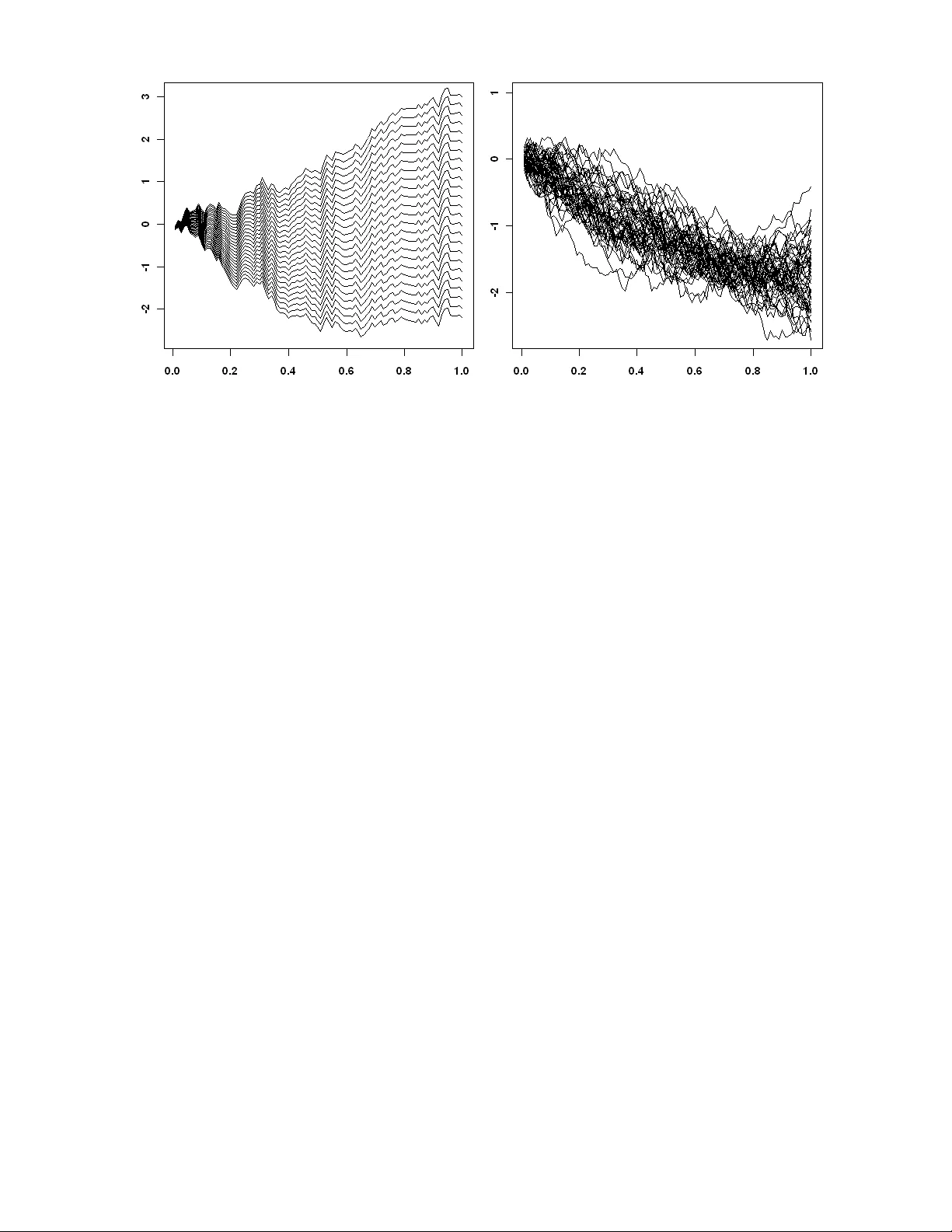
Nonparametric P ar tial Impor tance Sampling f or Financial Der iv ativ e Pr icing Jan C . Nedder mey er ∗ Abstract. Impor tance sampling is a promising variance reduction technique f or Monte Carlo simulation based deriv ativ e pr icing. Existing impor tance sampling methods are based on a parametric choice of the proposal. This ar ticle proposes an algorithm that estimates the optimal proposal nonparametrically using a multivariate frequency polygon estimator . In contrast to parametric methods, nonpar ametric estimation allows f or close approximation of the optimal proposal. Standard nonpar ametric impor tance sampling is inefficient f or high- dimensional problems. We solve this issue by applying the procedure to a low-dimensional subspace, which is identified through pr incipal component analysis and the concept of the eff ectiv e dimension. The mean square error proper ties of the algorithm are inv estigated and its asymptotic optimality is shown. Quasi-Monte Carlo is used f or fur ther impro vement of the method. It is easy to implement, par ticularly it does not require any analytical computa- tion, and it is computationally very efficient. W e demonstrate through path-dependent and multi-asset option pricing prob lems that the algor ithm leads to significant efficiency gains compared to other algorithms in the literature. Ke yw ords. Asian option; Effectiv e dimension; Nonparametric density estimation; Nonpara- metric impor tance sampling; Option pricing; P ath-dependent option; Quasi-Monte Car lo; V ariance reduction ∗ University of Heidelberg, Institute of Applied Mathematics , Im Neuenheimer F eld 294, D-69120 Heidelberg, Germany (e-mail: jc@neddermey er .net). This work has been suppor ted by the Deutsche Forschungsgemein- schaft (D A 187/15-1). 1. INTRODUCTION In the last decade, the complexity of the pricing models used f or e valuation of financial prod- ucts e xperienced a distinct increase. As a consequence of this de v elopment, pure numeri- cal methods became more and more inadequate f or the arisen high-dimensional integr ation tasks. Often, Monte Car lo (MC) integration is the only f easib le method. This stems from the f act that the MC conv ergence rate is independent of the prob lem dimension. Howe ver , cr ude MC is often inefficient f or practical sample sizes. Raising computing power and increasing the sample size is no solution. The need of efficient MC procedure is apparent. T o make MC algorithms comparable , it is useful to quantify the efficiency of an estimator . Let’ s assume X is a random v ariable defined on a probability space (Ω , B , P ) and it is used to estimate some quantity µ . The computational efficiency (CE) of estimator X can be defined through CE [ X ] = ( MSE [ X ] C [ X ]) − 1 , where MSE [ X ] denotes the mean square error of X and C [ X ] the av erage costs of comput- ing one realization of X (L ’Ecuyer 1994). F rom this definition one obser v es that efficiency improv ements can be achiev ed either b y reducing the MSE or the computational costs. The f ormer includes well-known v ariance reduction (VR) techniques such as impor tance sampling (IS), antithetic sampling, moment matching, and control variates (Jäck el 2002; Glasser man 2004; Rober t and Casella 2004). Most VR techniques aim at improving a giv en set of samples, that is used f or MC integration. In contrast, IS is based on changing the distribution from which the samples are dr a wn. The idea behind IS is to select a distr ibu- tion (which is known as proposal) that forces the samples into the domain which is most impor tant to the integrand. Intuitively , this is particular ly useful f or derivativ es that rely on rare e v ents. A deep out-of-the money option is an obvious example f or rare ev ent depen- dency . Crude MC would only rarely produce samples which lead to non-zero pay outs and, consequently , the MC variance would be sev ere. Howe ver , IS is by far not limited to rare e v ent cases. Compared to other VR techniques the usage of IS is more inv olved, because the selection of a suitable proposal is generally difficult. But the additional effor t is justified by the large potential of IS to reduce the MC v ar iance. IS has been successfully applied to der iv ativ e pricing based on Gaussian proposals. That is, the proposal was chosen from some class of Gaussian distributions. An impor tant ap- proach is based on a mean shift, which can be obtained through saddle point appro xima- tion (Glasser man, Heidelberger , and Shahabuddin 1999), adaptive stochastic optimization (V azquez-Abad and Dufresne 1998; Su and Fu 2000, 2002), or least squares (Capriotti 2008). This approach is also known as the “change-of-drift technique”. In addition, Gaussian 1 mixture distr ibutions hav e been utilized for appro ximating the optimal proposal (A vramidis 2002). Summarizing, existing approaches are based on parametric IS, that is the proposal is chosen from a cer tain class of distributions. For complex pay outs it is hard to set up a class which contains a distribution that appro ximates the optimal proposal reasonably well. This paper proposes the usage of nonparametric IS (NIS) f or deriv ativ e pricing. The basic idea of NIS is to use a nonparametric estimate of the optimal proposal. NIS algorithms hav e already been successfully applied to low-dimensional integration problems (Giv ens and Rafter y 1996; Zhang 1996; Kim, Roh, and Lee 2000; Nedder meyer 2009). Howe ver , high-dimensional integration tasks hav e not been considered until now . As a result of the curse of dimensionality and computational limitations NIS cannot be applied directly to high- dimensional derivativ e pricing. We suggest to restr ict NIS to those coordinates that are of most impor tance to the integration problem. This approach can be justified by the concept of the effectiv e dimension (ED). T o reduce the effectiv e dimension and to identify the most rele v ant coordinates principal component analysis (PCA) is applied. The adv antage of NIS compared to parametric IS is its close appro ximation of the optimal proposal. W e prov e that the VR factor of our nonparametr ic method increases with sam- ple size conv erging to the - in some sense - optimal value . Note, parametr ic IS methods achie v e constant VR f actors. It is shown through simulations that the proposed algor ithm is computationally more efficient than parametric IS f or well-known benchmar k option pricing problems . In the case of low ED , the algorithm does not only outperform in ter ms of MSE but also in ter ms of computational costs. In other words, it is not only more accurate but also computationally cheaper . In addition, it is easy to implement based on the C ++ im- plementation of the nonparametric estimator which is provided. NIS and most parametric IS methods share the proper ty that they can be combined with other VR techniques. This is demonstrated through the use of low-discrepancy sequences (also known as quasi-MC (QMC)). This paper is organized as f ollows . In the ne xt section, a general MC option pr icing frame work is introduced and IS is briefly revie wed. In Section 3, a nonparametr ic par tial IS algorithm is proposed and its MSE conv ergence proper ties are inv estigated. The concept of the ED is re viewed in Section 4. In Section 5, path construction based on PCA is discussed, f ollow ed by a br ief introduction to QMC (Section 6). A compar ison to parametric IS is pre- sented in Section 7 and a detailed description of the implementation is given in Section 8. Finally , in Section 9 simulation results are repor ted f ollowed b y conclusions (Section 10). 2 2. DERIV A TIVE PRICING AND IMPOR T ANCE SAMPLING Let’ s describe the e volution of the underlying asset through a stochastic diff erential equa- tion (SDE) of the f orm dS ( t ) = rS ( t ) dt + σ ( S ( t )) S ( t ) dW ( t ) , (1) where W ( t ) is a standard Brownian motion (BM); r and σ are the r isk-free interest rate and the v olatility , respectiv ely . Within this model, e v aluating the pr ice of a European option with pa y out function C K ( S ) , strike le vel K , and e xpiry T means computing E [exp( − r T ) C K ( S )] , (2) where the e xpectation is taken with respect to the risk neutral measure. Except of special cases, there is no explicit solution for SDEs of kind (1). Theref ore, it is required to migrate to some discretization ˜ S t k of the process S ( t ) , which is defined on a discrete time grid 0 = t 0 < t 1 < · · · < t d = T . The first order Euler discretization scheme yields ˜ S t k +1 = ˜ S t k + r ˜ S t k ( t k +1 − t k ) + σ ( ˜ S t k ) ˜ S t k p t k +1 − t k Z t k (3) with standard nor mal innov ations Z t k . In the f ollowing, we focus on an equally-spaced time grid, i. e. t i − t i − 1 = ∆ t = const. Based on this discretization, the option pr ice (2) can be appro ximated through the integr al I ϕ = Z R d ϕ ( x ) p ( x ) d x , where ϕ ( x ) = exp( − rT ) C K ( ˜ S ( x )) . p denotes the density of the multivariate Gaussian distri- bution N ( 0 , I d ) with I d being the identity matr ix of dimension d . By writing ˜ S ( x ) , it is meant that a trajector y of ˜ S t k is built up based on the innov ations x = ( x 1 , . . . , x d ) T . T o keep the discretization bias small, it is required to choose d considerably large which leads to a high-dimensional integration prob lem. The crude MC estimator is given b y ˆ I MC ϕ = 1 N N X i =1 ϕ ( x i ) , where x 1 , x 2 , . . . , x N are dra wn from p . The estimator’ s large v ariance renders it impractical f or appro ximating comple x integrals . T o constr uct a more efficient MC estimator , IS can be applied. The basic idea of IS is to sample from a proposal q instead of p . The IS estimator is defined through ˆ I IS ϕ = 1 N N X i =1 ϕ ( x i ) w ( x i ) , 3 with likelihood ratio w ( x ) = p ( x ) /q ( x ) and samples x 1 , x 2 , . . . , x N dra wn from q . For ˆ I IS ϕ to conv erge to I ϕ , it is required that the suppor t of q includes the suppor t of | ϕ | p . Under the additional assumption V ar q [ ϕw ] < ∞ , a central limit theorem holds √ N ( ˆ I IS ϕ − I ϕ ) ⇒ N (0 , σ 2 IS ) , where σ 2 IS = E q [ ϕw − I ϕ ] 2 (Rubinstein 1981). This result allows the constr uction of confi- dence inter vals f or ˆ I IS ϕ and establishes the conv ergence rate O ( N − 1 / 2 ) . The optimal pro- posal, which minimizes the (asymptotic) v ar iance σ 2 IS , is giv en by q opt ( x ) = | ϕ ( x ) | p ( x ) R | ϕ ( x ) | p ( x ) d x . Remarkably , the IS estimator based on the optimal proposal q opt has zero variance f or func- tions ϕ with a definite sign. How e ver , the optimal proposal is unav ailable in practice because of its unknown denominator . 3. NONP ARAMETRIC P ARTIAL IMPOR T ANCE SAMPLING In this section, nonparametric par tial IS (NPIS) is introduced as a generalization of the NIS algorithm discussed in Zhang (1996) and Neddermeyer (2009). NIS is a two-stage procedure. In the first stage, the optimal proposal is estimated nonparametrically based on samples drawn from a tr ial distribution q 0 . In the second stage, this nonparametric density estimate is used as proposal for IS. We pick up this approach, but instead of approximat- ing the optimal proposal in the entire space, we focus on the optimal proposal in a cer tain subspace. That is, the nonparametric IS procedure is restr icted to a low-dimensional sub- problem in order to av oid the curse of dimensionality . We decompose x = ( x u , x − u ) , where u ⊆ { 1 , 2 , . . . , d } . The cardinality of u is denoted by | u | . Let’ s consider the marginalized optimal proposal obtained through integration with respect to x − u . It is given b y ˘ q opt ( x u ) = Z R d −| u | q opt ( x ) d x − u . Subspace u is chosen such that it cov ers those coordinates which are most impor tant to the integrand (see Section 4). T o limit the computational burden of the nonparametric method, u will be considerably small in practice ( 1 ≤ | u | ≤ 3 ). In the NPIS algor ithm, ˘ q opt is es- timated nonparametrically . Now , the choice of the nonparametric estimator is discussed. T ypically , kernel estimators hav e been used within NIS algor ithms. Howe ver , sampling and e v aluation is computationally v er y inefficient for kernel estimators. In this ar ticle , a multi- v ariate variant of the nonparametr ic frequency polygon estimator is used, which is known as linear blend frequency polygon (LBFP) (T errell 1983). The LBFP estimator attains the 4 same MSE conv ergence rate as ker nel estimators, namely O ( N − 4 / (4+ d ) ) , but it is com- putationally more efficient. The generation and the ev aluation of N samples is of order O (2 d − 1 d 2 N ( d +5) / ( d +4) ) (Neddermey er 2009), whereas kernel estimators require O ( dN 2 ) op- erations . The construction of an LBFP consists of inter polations of the bin mid-points of a multiv ar iate histogram. Let’ s consider a multiv ariate histogram estimator with bin height ˆ f H k 1 ,...,k d f or bin B k 1 ,...,k d = Q d i =1 [ t k i − h/ 2 , t k i + h/ 2) , where h is the bin width and ( t k 1 , . . . , t k d ) the bin mid-point. For x ∈ Q d i =1 [ t k i , t k i + h ) the LBFP estimator is defined as ˆ f ( x ) = X j 1 ,...,j d ∈{ 0 , 1 } " d Y i =1 x i − t k i h j i 1 − x i − t k i h 1 − j i # ˆ f H k 1 + j 1 ,...,k d + j d . (4) In the one-dimensional case , ˆ f is just a linear ly interpolated histogram. It can be shown that it integrates to one . Algorithm - Nonparametric P artial Impor tance Sampling Stage 1: Nonparametric estimation of the marginalized optimal proposal • Select subset u , bin width h , trial distr ibution q 0 , and sample sizes M and N . • For j = 1 , . . . , M : Generate sample ˜ x j ∼ q 0 . • Obtain nonparametric estimate ˆ q opt of marginalized optimal proposal ˘ q opt ˆ q opt ( x u ) = ˆ f ( x u ) 1 M P M j =1 ω j , where ω j = | ϕ ( ˜ x j ) | p ( ˜ x j ) q 0 ( ˜ x j ) − 1 and ˆ f ( x u ) = 1 M X j 1 ,...,j | u | ∈{ 0 , 1 } " Y i ∈ u x i − t k i h j i 1 − x i − t k i h 1 − j i # × M X j =1 ω j 1 Q i ∈ u [ t k i + j i − h/ 2 ,t k i + j i + h/ 2) ( ˜ x j ) f or x u ∈ Q i ∈ u [ t k i , t k i + h ) . Stage 2: P ar tial Impor tance Sampling • For i = 1 , . . . , N : Generate samples x i u ∼ ˆ q opt ( x u ) and x i − u ∼ p ( x − u ) . • Ev aluate ˆ I NPIS ϕ = 1 N N X i =1 ϕ ( x i ) p ( x i u ) ˆ q opt ( x i u ) − 1 . The f ollowing theorem inv estigates the MSE conv ergence proper ties of the NPIS algorithm to obtain the optimal v alue f or bin width h . 5 Theorem 1. Suppose that the assumptions given in Appendix A hold, ϕ ≥ 0 , and p ( x ) = p ( x u ) p ( x − u ) . We denote ˘ q = ˘ q opt . Then, we obtain f or ˆ I NPIS ϕ M (as defined in Appendix A) E [ ˆ I NPIS ϕ M − I ϕ ] 2 = 1 N " Z ν ( x ) 2 p ( x − u ) ˘ q ( x u ) d x + I 2 ϕ ( h 4 H 1 + 2 | u | 3 | u | M h | u | H 2 ) × (1 + o (1)) # (5) and the optimal bin width h opt = | u | H 2 2 | u | 4 H 1 3 | u | ! 1 4+ | u | M − 1 4+ | u | , where H 1 = 49 2 , 880 X i ∈ u Z ( ∂ 2 i ˘ q ) 2 ˘ q + 1 64 X i,j ∈ u i 6 = j Z ∂ 2 i ˘ q ∂ 2 j ˘ q ˘ q , H 2 = Z ( q opt ) 2 ˘ q q 0 and ν ( x ) = ϕ ( x ) p ( x u ) − Z ϕ ( x ) p ( x ) d x − u . Proof. See Appendix A. The left and right ter m in the brack ets in (5) can be inter preted as the variance caused by the components x − u and x u , respectively . Note, subset u is chosen such that the left ter m is small compared to the right one. The e xpression in braces quantifies the MSE of the nonparametric estimate, which depends on both ˘ q opt and tr ial distr ibution q 0 . For h = h opt and M / N → λ ∈ (0 , 1) ( M , N → ∞ ) the theorem implies E [ ˆ I NPIS ϕ M − I ϕ ] 2 = 1 N Z ν ( x ) 2 p ( x − u ) ˘ q ( x u ) d x + O ( N − (8+ | u | ) / (4+ | u | ) ) . Hence, the variance caused by x u is of lower order . In other words, the optimal vari- ance (for par tial IS on coordinates u ) is achie v ed asymptotically . As a consequence, com- pared to crude MC and parametric IS techniques, NPIS is e xpected to yield increasing ef- ficiency as the sample size grows. Fur ther more, if | u | = d the MSE conv erges as fast as O ( N − (8+ d ) / (4+ d ) ) , which is a massive improvement compared to the standard MC rate O ( N − 1 ) , for d that is small (Zhang 1996; Nedder mey er 2009). Note, the results of this section also hold f or distributions p other than the standard nor mal distr ibution. In this ar ticle, NPIS is only inv estigated for non-negativ e integrands . Howe ver , by decom- posing the pa yout function C = C + − C − , NPIS can also be applied to financial derivativ es that hav e both positive and negativ e pay outs. 4. EFFECTIVE DIMENSION The NPIS algor ithm is based on the restriction on specific coordinates x u , where in high- dimensional integration problems | u | d . This approach can be justified by the concept 6 of the ED . It is well known, that many integration problems in financial engineering, despite having a large nominal dimension, are low-dimensional in ter ms of the ED . For a r igorous definition of the ED , let’ s consider the functional analysis of v ariance (ANO V A) decomposi- tion. Suppose R ϕ ( x ) 2 p ( x ) d x < ∞ and p ( x ) = Q d i =1 p ( x i ) is a product density . Then, ϕ can be written as a sum of 2 d or thogonal functions ϕ ( x ) = X u ⊆{ 1 , 2 ,...,d } ϕ u ( x u ) , where the ANO V A functions ϕ u are giv en recursiv ely by ϕ u ( x u ) = Z R d −| u | ϕ ( x ) p ( x − u ) d x − u − X v ⊂ u ϕ v ( x v ) . Now , the fraction of the variance σ 2 = V ar p [ ϕ ] , that is e xplained by cer tain lower-dimensional ANO V A functions, is considered. F or this pur pose, the variance of ϕ u is defined by σ 2 u = R R d ϕ u ( x u ) 2 p ( x ) d x , where σ 2 ∅ = 0 . As the ANO V A decomposition is or thogonal, one has σ 2 = P u σ 2 u . Hence , Γ u = P v ⊆ u σ 2 v can be interpreted as the contr ibution of x u to the total variance of ϕ . F or a more detailed descr iption of the ANO V A decomposition see, f or instance, T akem ura (1983) and Owen (1992). The follo wing definition of the ED is due to Caflisch, Morokoff , and Owen (1997). Definition 1. The ED (in the tr uncation sense) is the cardinality of the smallest subset u such that Γ u ≥ γ σ 2 with 0 < γ < 1 . The threshold γ is chosen close to one. In the frame wor k of this ar ticle , we f ound γ = 0 . 9 reasonable . The ED does not only allow to identify those coordinates which most effect the integral value but it also indicates how many coordinates are required to cov er a cer tain amount of the variance. An MC procedure that allows one to determine the ED of a given problem is described in Appendix B . 5. GA USSIAN MODELS The purpose of this section is to show how NPIS can be applied to models that are based on the integration with respect to high-dimensional Gaussian distr ibutions . As mentioned bef ore, NPIS is inefficient as a result of the curse of dimensionality unless the ED (and thus | u | ) is small. For typical financial integration problems it is generally not advisable to apply NPIS with | u | larger than 3, unless the number of paths to be sampled is huge or the domain of interest is v er y small (rare e vent case). 7 Suppose the task is to integrate with respect to N (0 , Σ) . Now , PCA is used to transf or m the problem. The (positive-definite) cov ar iance matrix Σ is wr itten as Σ = V Λ V T , with Λ = diag ( λ 1 , λ 2 , . . . , λ d ) and eigenv alues λ i . The columns of V are the corresponding unit-length eigenv ectors. Thus, one has V Λ 1 / 2 Z ∼ N (0 , Σ) for Z ∼ N (0 , I d ) . Without loss of generality , it is assumed that the eigenv alues (and the corresponding eigenv ectors) are sor ted so that λ 1 ≥ λ 2 ≥ · · · ≥ λ d . The PCA constr uction of samples from N (0 , Σ) is optimal in the sense that it provides an optimal lower-dimensional approximation (in the MSE sense) to the random variable of interest. This means that the first k components of Z e xplain as much as possible of the total v ariance. More precisely , it can be sho wn that the y explain the fraction ( λ 1 + λ 2 + . . . + λ k ) / ( λ 1 + λ 2 + . . . + λ d ) . The option pricing prob lem introduced in Section 2 leads to the constr uction of discretized BM paths based on samples from the multiv ariate Gaussian distr ibution. P aths are most easily b uild up through the random w alk construction guided b y (3). In this constr uction each component “counts roughly the same” render ing the restriction on a lower-dimensional subspace and hence the application of NPIS impr actical. Note, the integ ral I ϕ can be rewrit- ten as I ϕ = R ˜ ϕ ( x ) p N ( 0 , Σ) ( x ) d x , where Σ is the cov ariance matrix of the discretized BM with entries Σ ij = min { t i , t j } . This suggests that PCA can be used to reduce the ED . The PCA construction of discretized BM paths has a continuous limit known as Karhounen-Loève e xpansion of BM: W ( t ) = ∞ X i =1 p λ i ψ i ( t ) Z i , 0 ≤ t ≤ 1 , where ψ i ( t ) = √ 2 sin { ( i − 0 . 5) π t } , λ i = { ( i − 0 . 5) π } − 2 , and Z i ∼ N (0 , 1) (Adler 1990). Based on the e xpression for λ i , it is easily shown that Z i e xplains the fraction 2 λ i of the path’ s v ariability (which is approximately 81%, 9%, 3% for i = 1 , 2 , 3 , respectively). These values are not only of asymptotic nature but also hold for a small number of discretization steps (with slight de viations). This astonishing result claims that very f ew PCA components suffice to deter mine most of the path’ s variation no matter how long or detailed it is. Particular ly , the first PCA component plays a dominant role and has a nice geometr ical inter pretation. Roughly speaking, it deter mines the path’ s direction in the path space. This is visualized in Figure 1. Another common method for the reduction of the ED (of a discretized BM) is the Brownian Bridge technique. In this paper , the focus is on PCA because of its optimality proper ty . How e v er , it is remarked that in cer tain situations Brownian Br idge techniques are super ior to PCA. This ma y especially be the case if the pa yout function only depends on the terminal v alue of the underlying. Note, NPIS can also be combined with Brownian Br idge techniques. 8 Figure 1: Discretized BM paths: first PCA component v aries whereas other components are fixed to random values (left); first PCA component is fix ed and other components vary randomly (right). 6. QU ASI-MONTE CARLO INTEGRA TION QMC is often used to (fur ther) improv e MC estimators. In contrast to MC , QMC integration uses so-called low-discrepancy sequences instead of (pseudo-) random numbers. Low- discrepancy numbers are constructed to fill the space more e venly . For a description of the construction of low-discrepancy sequences readers are referred to Niederreiter (1992), Glasser man (2004), and the ref erences given there. The incentive to work with QMC is justified by its deter ministic error bound of order O ( N − 1 log d N ) , which f ollows from the well-kno wn Koksma-Hla wka inequality (see Niederreiter (1992)). This bound is merely of theoretical benefit because the computation of the inv olv ed constants (including the Hardy- Krause v ariation of the integrand) is inf easible or at least v ery difficult. Howe ver , it suggests that QMC should massively outperform MC in low-dimensional integration problems . The adv antage of QMC diminishes with increasing dimension. Nev er theless, it is well known in the financial engineer ing literature , that QMC ma y be eff ectively applied to high-dimensional problems (P askov and T raub 1995; Ninomiya and T ezuka 1996; T raub and Werschulz 1998). This stems from the f act mentioned ear lier that many problems in finance hav e rather low ED compared to the nominal dimension. As the con v ergence proper ties of QMC become worse in higher dimensions, it is impor tant to assign the first coordinates to the most rele v ant dimensions of the integration problem. In our setting, the rele vant coordinates are those contained in u . A drawbac k of QMC is the lack of randomness, which impedes the computation of the MSE for assessing the accur acy of the estimator . This issue can be resolved b y randomizing the deter ministic low-discrepancy sequence to achie v e independent realizations of the QMC 9 estimator . Diff erent approaches for randomizing low-discrepancy sequences are av ailable including Owen’ s scramb ling (Owen 1995), random digit scramb ling (Matoušek 1998), or random shifts (see Ökten and Eastman (2004) for a sur ve y). In our simulations, prior ity is given to the random shift technique because of its straightf orw ard implementation. The idea is to shift the entire sequence by a random vector v modulo one. v is dra wn from the unif orm distr ibution on [0 , 1) d . That is, a randomized sequence is obtained by substituting the quasi-random v ectors y i of the original low-discrepancy sequence by ( y i + v ) mod 1 . 7. COMP ARISON T O P ARAMETRIC IMPOR T ANCE SAMPLING Until now , the application of IS in finance w as limited to par ametric IS . In particular , Gaus- sian or mixtures of Gaussian distr ibutions hav e been applied. The variance of a parametric IS estimator with proposal q θ (and parameter θ ∈ Θ ) can be wr itten as σ 2 IS N = I 2 ϕ N Z R d q opt ( x ) 2 q θ ( x ) d x − 1 , (6) where σ 2 IS is defined as in Section 2. First, this suggests that, in contrast to NPIS, the VR f actor is constant because all ter ms are O ( N − 1 ) . Second, the variance is cr itically affected by the tails of q θ . Using Gaussian proposals, it is often hard to appro ximate the tails of q opt reasonably well. There lies a distinct advantage of NIS methods. Most parametric IS approaches aim at choosing θ so that (6) is minimized. We now discuss a variant of the least-squares IS (LSIS) algorithm (Capr iotti 2008) which is directly comparab le to NPIS. It is based on the Gaussian proposal N ( µ, I d ) with parameter µ ∈ R d . Similar to NPIS, it is a two-stage algorithm. In the first stage, based on M samples from p , a least-squares problem is solv ed to estimate the optimal drift change µ . (The variance can also be adjusted through this procedure.) Howe ver , as the problem dimension grows the estimate of µ becomes unre- liable . The v ariant of this algorithm which is suggested here applies LSIS to the coordinates x u , that are deter mined through PCA and the ED (analogous to NPIS). This makes the LSIS and the NPIS directly comparable . In Section 9, NPIS and this variant of LSIS are tested against each other through simulations . Besides the super ior conv ergence proper ties NPIS has a computational advantage over parametric IS which is of relev ance in practice. For computing the IS weights, parametric IS typically needs to e v aluate the exp function which is very e xpensiv e. Through the use of the LBFP estimator , these e v aluations are reduced in the NPIS algor ithm. This leads to a rele v ant reduction of the computational costs (compare Section 9). 10 Finally , w e remark that combinations of parametric IS and NPIS are possib le. F or in- stance, while applying NPIS to x u one can carr y out parametr ic IS on the remaining coordi- nates x − u . 8. IMPLEMENT A TION OF THE ALGORITHM In this section, the details of practical implementation of the proposed NPIS algor ithm is discussed. At first, an ov er view ov er the required ingredients f or the implementation is given. 8.1 O VER VIEW Subset u : This is chosen according to the ED ( γ = 0 . 9 ), which can be computed with the algorithm given in Appendix B. If PCA is used, the first f ew pr incipal components are selected. T rial distribution q 0 : The choice of the trial distr ibution should be guided by the f ollow- ing two criter ia: First, it should allow for efficient sampling and ev aluation. Second, the marginal distr ibutions of the coordinates contained in u should be ov erdispersed (heavy tailed) compared to the standard normal distribution. An all-pur pose trial distri- bution, which we found to work well in practice, is discussed in Subsection 8.2. Alter- nativ ely , one can use a parametric choice tailored to the specific integration problem or one can simply use the (multivariate) standard nor mal distribution. The latter is often not a good choice because of the impor tance of the tails of the proposal. Bin width h : A Gaussian reference r ule can be computed in Stage 1 of the algor ithm (for details see Subsection 8.3). Sample size M : F or the simulations , we used M = max { 256 , 0 . 25 N } . In the special case when | u | = d an optimal value f or the propor tion M / N can be derived (Zhang 1996; Nedder mey er 2009). LBFP estimator: The details of the implementation of the LBFP estimator can be f ound in Nedder mey er (2009). A C ++ implementation of the LBFP as well as the R-package lbfp are av ailable on request. W e emphasize that, in contrast to most parametric IS algor ithms, all parameters are ad- justed automatically , such that no trial-and-error parameter selection and no analytical com- putation are necessar y in practice. 11 8.2 TRIAL DISTRIBUTION As tr ial distribution we propose a simple product density . It is composed of a unif orm distribution on [ − ρ M , ρ M ] | u | and the multiv ar iate Gaussian distr ibution p ( x − u ) : q 0 ( x ) = p ( x − u ) × 1 (2 ρ M ) | u | Y i ∈ u 1 [ − ρ M ,ρ M ] ( x i ) , where ρ M is the (1 + (1 − ) 1 / M ) / 2 -quantile of N (0 , 1) . > 0 is v er y small, say = 10 − 4 . Consequently , P (max 1 ≤ i ≤ M | Z i | > ρ M ) = holds for standard nor mal distr ibuted Z i . This ensures that the bias caused by the bounded suppor t of the uniform distr ibution is very small. In addition, the unif or m distr ibution guaranties that the space of x u is well e xplored e v en f or a small sample size. 8.3 PRA CTICAL BIN WIDTH SELECTION The expression f or h opt giv en in Theorem 1 is intractabl e analytically because of the un- known constants H 1 , H 2 . The plug-in method suggested in Zhang (1996) also seems un- suitable for our integr ation problem as derivativ es of the integr and are required. We propose to apply a Gaussian approximation of H 1 , H 2 . Suppose ˘ q opt is the density of a centered multiv ar iate Gaussian distr ibution with cov ariance matr ix diag ( σ 2 1 , σ 2 2 , . . . , σ 2 | u | ) . Under this assumption, it can be shown that H 1 = 98 2 , 880 X i ∈ u σ − 4 i . (7) F or the constant H 2 the mean of q opt pla ys the dominant role. Therefore , it is assumed that q opt is the density of N (( µ 1 , µ 2 , . . . , µ d ) T , I d ) . If the tr ial distribution is chosen as e xplained in the preceding subsection, one yields H 2 ≈ ρ | u | M exp[ X i / ∈ u µ 2 i ] . (8) In the algor ithm, the expressions in (7) and (8) can be approximated based on the sam- ples ˜ x 1 , . . . , ˜ x M . This f ollows from the fact, that the samples ˜ x j weighted with ω j / P M k =1 ω k appro ximate q opt . 9. SIMULA TION RESUL TS Diff erent European option pricing scenar ios are considered to compare the proposed al- gorithms (NPIS and the combination of NPIS and QMC (QNPIS)) with existing methods (crude MC, QMC , LSIS, and the combination of LSIS and QMC (QLSIS)). The perf ormance 12 of the algorithms is measured through the VR factors (computed with respect to crude MC) and the relative computational efficiency (RCE). The RCE is defined as the ratio of the CE of the method of interest to the CE of cr ude MC. The computational costs are measured in seconds. All simulations are done for different sample sizes N in order to demonstrate the increasing VR f actors of NPIS . Examples 1 through 3 consider different single- and multi-asset options within the stan- dard Black-Scholes model. There, the price of an asset S at time t is given b y S ( t ) = S (0) exp[( r − 0 . 5 σ 2 ) t + σ √ tZ ] with standard normal random variab le Z . The simulations are based on the f ollowing setting: S (0) = 100, σ = 0 . 3 , r = 0 . 05 , and T = 1 . In Example 4, the pricing of a cap within the CIR model is inv estigated to show the eff ectiveness of NPIS/QNPIS in a square-root diffusion model. For all algor ithms, apar t from cr ude MC , the PCA path constr uction is used. The parameters u , q 0 , and h are chosen according to the description in the preceding section. Note, Theorem 1 does not apply to QMC sampling. We f ound empirically that QNPIS requires a larger bin width. In the simulations , 3 h opt is used. For LSIS and NPIS, M is set as suggested in the preceding section whereas for QNPIS and QLSIS M = 1024 is used throughout. The least squares estimates required in LSIS/QLSIS were computed with ten iterations of the Le venberg-Marquardt method (Press et al. 1992, pp . 683-688). The computations were carried out on a Dell Precision T3400, Intel CPU 2.83GHz. All algorithms were coded in C ++ . The Mersenne T wister 19937 (Matsumoto and Nishimura 1998) and the Sobol sequence (Sobol 1967) were used f or pseudo- and quasi-random num- ber generation, respectively . The Sobol sequence is randomized by the random shift tech- nique. The transf ormation of unif orm random numbers into nor mal random numbers was done by the Beasle y-Spr inger-Moro appro ximation (Moro 1995). Example 1. Straddle Option The pa y out function of a straddle option is giv en by C K ( S ) = ( S ( T ) − K ) + + ( K − S ( T )) + . In the Black-Scholes world the pr icing of a straddle option is a one-dimensional integration problem with multi-modal optimal proposal. Gaussian proposals (such as drift changes) are se v erely inefficient for multi-modal pay outs (Capr iotti 2008). The optimal proposal and an LBFP estimate generated in the NPIS algor ithm are shown in Figure 2. The LBFP estimate closely appro ximates the optimal proposal. T o account for the bimodality , we used 2 h opt as 13 Figure 2: Standard nor mal distribution (dotted line), optimal proposal f or a straddle option within the Black- Scholes model (dashed line), and an LBFP estimate of the optimal proposal (solid line). Model parameters: S (0) = 100, σ = 0 . 3 , r = 0 . 05 , T = 1 , and K = 100. P arameters VR (RCE) N K QMC LSIS NPIS QLSIS QNPIS 2 10 100 224 (380) 1.3 (0.4) 9 (0.9) 1,064 (127) 2.3 × 10 5 (8,469) 110 253 (548) 1 (0.4) 6 (0.8) 964 (150) 3.2 × 10 5 (1.5 × 10 4 ) 2 11 100 264 (557) 1.3 (0.5) 13 (1.7) 1,361 (384) 2.6 × 10 5 (2.1 × 10 4 ) 110 290 (532) 1 (0.3) 8 (1) 1,092 (291) 3.1 × 10 5 (2.4 × 10 4 ) 2 12 100 460 (941) 1.3 (0.4) 17 (2.2) 2,209 (1,006) 6.8 × 10 5 (8.6 × 10 4 ) 110 505 (953) 1 (0.3) 11 (1.3) 2,201 (965) 7.4 × 10 5 (8.7 × 10 4 ) T able 1: The table repor ts the variance reduction (VR) f actors and the relativ e computational efficiency (RCE) f or a straddle option within the Black-Scholes model. Model parameters: S (0) = 100, σ = 0 . 3 , r = 0 . 05 , T = 1 , and | u | = d = 1 . All values are computed based on 1,000 independent runs. bin width in the QNPIS algor ithm. How e v er , 3 h opt giv es only slightly worse results. The simulation results f or the strikes K = 100 and K = 110 are repor ted in T able 1. First notice, that NPIS significantly outperf orms LSIS because of the better appro ximation of the optimal proposal. Second, the VR factors f or NPIS increase with sample size which agrees with Theorem 1. Third, the combination of NPIS and QMC leads to massiv e efficiency gains. Even after adjusting for the ex ecution times the gains are enor mous (see values for the RCE). Note, the increasing VR factors f or QLSIS and QNPIS are a result of the QMC sampling. Example 2. Asian Options An arithmetic Asian call with pay out function C K ( S ) = 1 d d X i =1 S ( t i ) − K ! + 14 is inv estigated. The optimal proposal is unimodal. This integration problem is w ell suited f or NPIS/QNPIS because its ED is one. The str ikes K = 100, 130, and 175 are considered. F or str ike K = 175 the option price is appro ximately 0.018 (for d = 16) representing a rare e v ent option pricing framew or k (which is still of practical interest). T able 2 shows the results for d = 16 and d = 64 discretization steps. The results of the Gaussian IS algorithm (GIS) based on saddle point approximation (Glasser man, Hei- delberger , and Shahabuddin 1999) are also repor ted. We emphasize that the VR and RCE increase with both str ike lev el K and the sample size. The VR f actors of GIS and LSIS are roughly constant. This coincides with the theoretical results. P ar ticularly in the rare e v ent cases, massive efficiency gains are achiev ed and NPIS/QNPIS improve significantly ov er their parametr ic competitors. In addition, the v alues f or RCE establish that NPIS and QNPIS are computationally much more efficient than parametric IS strategies. In the table, missing values indicate that the tr ial stage sometimes failed to generate paths with positiv e pa y outs. T o e xplain the result’ s dependency on the str ike lev el, the marginalized optimal proposal (of the first PCA component) f or different str ikes were plotted (Figure 3). One can obser ve that both the mean and the variance of the marginalized optimal proposals alter with K . As a result of the shr inking v ariance (and the increasing ske wness) of the marginalized optimal proposals, IS approaches based on pure dr ift changes become worse (relativ ely to NPIS/QNPIS) as K increases. T able 3 gives results for the case when the e x ecution time is fixed such as in real-time application. The sample sizes w ere chosen so that all algorithms needed appro ximately the same time for e x ecution. The values suggest that the v ariance of NPIS is roughly ten times smaller than those of e xisting IS techniques. In T able 4, the values f or an Asian option with a knoc k-out f eature are shown. The option will pay nothing if the ar ithmetic av erage e xceeds the knock-out le v el ˜ K . The pa y out function is giv en by C K ( S ) = 1 d d X i =1 S ( t i ) − K ! + 1 { 1 d P d i =1 S ( t i ) < ˜ K } . The ev aluation of this option is a difficult task because the rele v ant domain is very narrow . The str ike K = 140 and the knock-out le v els ˜ K = 150 and ˜ K = 170 are considered. The EDs are two and one for ˜ K = 150 and ˜ K = 170, respectively . Both LSIS and NPIS hav e problems to generate paths with positiv e pay outs in the trial stage (which is reflected in the missing v alues in T able 4). Again, QNPIS significantly improves o ver QLSIS . Finally , simulations for an Asian str addle option that pa ys C K ( S ) = ( 1 d d X i =1 S ( t i ) − K ) + + ( K − 1 d d X i =1 S ( t i )) + 15 Figure 3: Standard normal distr ibution (dotted line), marginalized optimal proposal (of first pr incipal compo- nent) for an Asian option with str ike K = 60 (solid line), K = 100 (dashed line), and K = 140 (heavy line). Model parameters: S (0) = 100, σ = 0 . 3 , r = 0 . 05 , T = 1 , and d = 16 . are discussed. As for the standard straddle option, NPIS provides efficiency gains compared with LSIS (see T ab le 5). Although, the VR f actors and the RCE of QNPIS are large , they are much smaller than those obtained f or the standard straddle option. Example 3. Multi-Asset Options In this e xample, multi-asset options are considered. Suppose one deals with s assets that satisfy S i ( t ) = S i (0) exp[( r − 0 . 5 σ 2 ) t + σ √ tZ i ] i = 1 , . . . , s, where the correlation matrix of Z 1 , . . . , Z s is denoted by Σ . T o keep the setting simple, S i (0) = 100 and corr ( Z i , Z j ) = 0 . 3 for i, j = 1 , . . . , s , i 6 = j is assumed. The ED is reduced by applying PCA to the correlation matr ix. W e inv estigate two different pay out structures. First, the price for an a verage option with pa yout C K ( S 1 , . . . , S s ) = 1 s s X i =1 S i ( T ) − K ! + is computed. The second option depends on the maximum of the under lyings’ final v alues and has the pa y out function C K ( S 1 , . . . , S s ) = max 1 ≤ i ≤ s { S i ( T ) } − K + . F rom T able 6, one can obser v e that the results f or the av erage option are qualitatively similar to those of the Asian option in Example 2. P ar ticular ly , the ED is also equal to one . 16 P arameters VR (RCE) N d K ED QMC GIS LSIS NPIS QLSIS QNPIS 2 10 16 100 1 139 (139) 10 (3) 9 (2) 21 (11) 1,427 (113) 859 (187) 140 1 17 (17) 55 (17) 50 (10) 200 (102) 4,778 (375) 5,462 (1,193) 175 1 2 (2) 683 (202) - (-) 3,809 (1,941) 4.3 × 10 4 (3,326) 1.1 × 10 5 (2.5 × 10 4 ) 64 100 1 145 (144) 8 (3) 8 (2) 20 (11) 1,409 (108) 909 (224) 140 1 16 (16) 61 (19) 53 (10) 245 (138) 5,679 (434) 7,428 (1,828) 175 1 2 (2) 902 (280) - (-) 4,403 (2,501) 5.8 × 10 4 (4,506) 1.0 × 10 5 (2.5 × 10 4 ) 2 11 16 100 1 171 (173) 9 (3) 9 (2) 28 (14) 1,535 (226) 908 (322) 140 1 21 (22) 57 (17) 52 (10) 285 (146) 5,647 (823) 6,443 (2,267) 175 1 3 (3) 680 (204) - (-) 5,161 (2,646) 4.5 × 10 4 (6,599) 1.3 × 10 5 (4.4 × 10 4 ) 64 100 1 185 (185) 9 (3) 9 (2) 30 (17) 1,583 (225) 912 (360) 140 1 21 (16) 69 (21) 55 (10) 329 (185) 5,951 (847) 8,027 (3,164) 175 1 2 (2) 1,072 (332) - (-) 7,255 (4,117) 6.2 × 10 4 (8,757) 1.1 × 10 5 (4.4 × 10 4 ) 2 12 16 100 1 339 (339) 9 (3) 9 (2) 33 (17) 2,549 (647) 1,499 (767) 140 1 42 (43) 56 (17) 59 (12) 324 (167) 8,742 (2,219) 1.0 × 10 4 (5,212) 175 1 5 (5) 756 (232) - (-) 5,224 (2,696) 8.7 × 10 4 (2.2 × 10 4 ) 2.2 × 10 5 (1.1 × 10 5 ) 64 100 1 354 (352) 10 (3) 10 (2) 35 (20) 2,743 (682) 1,627 (921) 140 1 36 (36) 68 (21) 57 (11) 369 (209) 9,685 (2,407) 1.3 × 10 4 (7,388) 175 1 4 (4) 1,031 (318) - (-) 7,414 (4,198) 9.7 × 10 4 (2.4 × 10 4 ) 1.8 × 10 5 (1.0 × 10 5 ) T able 2: The tab le repor ts the variance reduction (VR) f actors, the relativ e computational efficiency (RCE), and the effectiv e dimension (ED) for an Asian option within the Black-Scholes model. Model parameters: S (0) = 100, σ = 0 . 3 , r = 0 . 05 , T = 1 . All values are computed based on 1,000 independent runs. VR ( N ) Time ED MC GIS LSIS NPIS 0.35 1 1 ( 2 13 ) 16 ( b 2 11 . 19 c ) 12 ( b 2 10 . 68 c ) 168 ( 2 12 ) 0.7 1 1 ( 2 14 ) 16 ( b 2 12 . 19 c ) 11 ( b 2 11 . 68 c ) 175 ( 2 13 ) 1.4 1 1 ( 2 15 ) 17 ( b 2 13 . 19 c ) 11 ( b 2 12 . 68 c ) 158 ( 2 14 ) T able 3: The table reports the variance reduction (VR) factors , the sample sizes ( N ), and the effectiv e dimen- sion (ED) f or an Asian option within the Black-Scholes model. The e x ecution time is fix ed to 0.35, 0.7, and 1.4 seconds, respectively . The sample sizes are chosen such that all algor ithms appro ximately achiev ed the fixed e x ecution time. Model parameters: S (0) = 100, σ = 0 . 3 , r = 0 . 05 , T = 1 , K = 140, and d = 16. All values are computed based on 1,000 independent runs. P arameters VR (RCE) N ˜ K ED QMC LSIS NPIS QLSIS QNPIS 2 10 150 2 5 (5) - (-) - (-) 69 (5) 110 (21) 170 1 16 (16) - (-) 37 (19) 1,003 (80) 1,362 (297) 2 11 150 2 6 (6) - (-) - (-) 68 (10) 123 (36) 170 1 18 (18) - (-) 134 (68) 1,168 (171) 1,613 (568) 2 12 150 2 6 (6) - (-) - (-) 82 (21) 163 (63) 170 1 23 (24) - (-) 106 (55) 1,530 (394) 1,883 (961) T able 4: The table repor ts the variance reduction (VR) factors , the relative computational efficiency (RCE), and the effectiv e dimension (ED) for an Asian option with a knock-out feature within the Black-Scholes model. Model par ameters: S (0) = 100, σ = 0 . 3 , r = 0 . 05 , T = 1 , K = 140, and d = 16. All values are computed based on 1,000 independent runs. 17 P arameters VR (RCE) N d ED QMC LSIS NPIS QLSIS QNPIS 2 10 16 1 193 (199) 1.2 (0.2) 6 (3) 300 (24) 323 (71) 64 1 213 (214) 1.1 (0.2) 6 (4) 321 (25) 361 (90) 2 11 16 1 225 (233) 1.2 (0.2) 8 (4) 359 (53) 418 (151) 64 1 256 (249) 1.2 (0.2) 9 (5) 397 (57) 410 (164) 2 12 16 1 425 (440) 1.2 (0.2) 10 (5) 634 (165) 711 (372) 64 1 454 (455) 1.2 (0.2) 11 (6) 715 (179) 717 (406) T able 5: The table repor ts the variance reduction (VR) factors , the relative computational efficiency (RCE), and the estimated effectiv e dimension (ED) for an Asian straddle option within the Black-Scholes model. Model parameters: S (0) = 100, σ = 0 . 3 , r = 0 . 05 , T = 1 , and K = 100. All values are computed based on 1,000 independent runs. P arameters VR (RCE) N K ED QMC LSIS NPIS QLSIS QNPIS 2 10 100 1 179 (346) 9 (4) 24 (24) 4,048 (620) 3,315 (1,384) 140 1 19 (38) 43 (16) 212 (210) 5,171 (788) 6,269 (2,612) 175 1 2 (3) - (-) 3,277 (3,229) 2.5 × 10 4 (3,856) 4.5 × 10 4 (1.9 × 10 4 ) 2 11 100 1 212 (409) 9 (3) 34 (33) 4,249 (1,197) 3,677 (2,475) 140 1 26 (50) 48 (18) 338 (333) 5,438 (1,533) 6,932 (4,697) 175 1 2 (4) - (-) 4,637 (4,571) 2.9 × 10 4 (8,313) 4.9 × 10 4 (3.3 × 10 4 ) 2 12 100 1 428 (830) 9 (3) 49 (48) 4,872 (2,403) 3,996 (3,948) 140 1 49 (96) 52 (20) 372 (368) 6,373 (3,157) 7,720 (7,630) 175 1 4 (9) - (-) 5,953 (5,857) 4.3 × 10 4 (2.1 × 10 4 ) 6.5 × 10 4 (6.4 × 10 4 ) T able 6: The tab le repor ts the variance reduction (VR) f actors, the relativ e computational efficiency (RCE), and the estimated effectiv e dimension (ED) for a multi-asset average option within the Black-Scholes model. Model parameters: S i (0) = 100 ( i = 1 , . . . , s ), σ = 0 . 3 , r = 0 . 05 , T = 1 , and s = 16. All v alues are computed based on 1,000 independent runs. The results for the second option with str ikes K = 150 and K = 200 are repor ted in T ables 7 and 8, respectiv ely . The pr icing of the second option is a difficult problem because the ED is equal to the nominal dimension. Although, f or K = 200 QNPIS is superior to QMC and QLSIS f or s = 2, 3, and 4 (in ter ms of the VR f actors), for K = 150 this only holds f or s = 2 and 3. We emphasize on the massive efficiency gains obtained by QNPIS for str ike K = 200. F or s > 2 the sample size used was too small f or NPIS to perf orm well. We conclude that the applicability of NPIS/QNPIS depends not only on the ED of the prob lem but also on the sample size used. An LBFP estimate of the optimal proposal f or the case s = 2 is plotted in Figure 4. Here, the PCA construction leads to a bimodal optimal proposal which can be closely appro ximated though an LBFP . Example 4. Cap in the CIR model Finally , we consider the CIR interest rate model (Co x, Ingersoll, and Ross 1985). Here, interest rate r t f ollows a square-root diffusion model dr t = κ ( θ − r t ) dt + σ √ r t dW t . 18 Figure 4: LBFP estimate of the optimal proposal for the multi-asset max option with strike K = 150. Model parameters: S i (0) = 100 ( i = 1 , 2 ), σ = 0 . 3 , r = 0 . 05 , T = 1 , and | u | = 2 . P arameters VR (RCE) N s ED QMC LSIS NPIS QLSIS QNPIS 2 11 2 2 44 (68) 6 (1.8) 10 (0.6) 145 (33) 3,070 (228) 3 3 26 (56) 3 (1.2) 0.3 (0.02) 52 (14) 72 (7) 4 4 24 (41) 3 (1) 0.03 (0.002) 28 (7) 7 (0.5) 2 12 2 2 76 (136) 5 (1.9) 25 (1.6) 213 (91) 5,848 (620) 3 3 42 (79) 3 (1.2) 0.3 (0.02) 72 (32) 148 (16) 4 4 27 (45) 3 (1.1) 0.05 (0.002) 36 (16) 8 (0.7) 2 13 2 2 211 (391) 6 (2) 61 (4) 396 (270) 4.7 × 10 4 (5,916) 3 3 70 (119) 3 (1.1) 2 (0.08) 95 (65) 161 (20) 4 4 35 (60) 3 (1) 0.01 (0.001) 42 (30) 7 (0.7) T able 7: The tab le repor ts the variance reduction (VR) f actors, the relativ e computational efficiency (RCE), and the estimated eff ective dimension (ED) for a multi-asset max option with strike K = 150. Model parameters: S i (0) = 100 ( i = 1 , . . . , s ), σ = 0 . 3 , r = 0 . 05 , and T = 1 . All values are computed based on 1,000 independent runs. P arameters VR (RCE) N s ED QMC LSIS NPIS QLSIS QNPIS 2 11 2 2 8 (14) - (-) 49 (3) 65 (17) 7,997 (652) 3 3 4 (8) 2 (0.6) 0.2 (0.01) 17 (4) 165 (14) 4 4 5 (8) 0.8 (0.3) 0.1 (0.006) 9 (2) 20 (1.5) 2 12 2 2 13 (23) - (-) 163 (10) 82 (33) 1.8 × 10 4 (1,837) 3 3 7 (13) 4 (1.5) 3 (0.2) 22 (10) 259 (28) 4 4 6 (9) 4 (1.3) 0.2 (0.01) 11 (4.7) 24 (2.2) 2 13 2 2 32 (58) - (-) 304 (18) 95 (65) 1.1 × 10 5 (1.4 × 10 4 ) 3 3 11 (19) 5 (1.7) 1.2 (0.06) 28 (19) 292 (36) 4 4 8 (13) 4 (1.5) 0.05 (0.002) 13 (9.1) 27 (2.8) T able 8: The tab le repor ts the variance reduction (VR) f actors, the relativ e computational efficiency (RCE), and the estimated eff ective dimension (ED) for a multi-asset max option with strike K = 200. Model parameters: S i (0) = 100 ( i = 1 , . . . , s ), σ = 0 . 3 , r = 0 . 05 , and T = 1 . All values are computed based on 1,000 independent runs. 19 P arameters VR (RCE) N T K ED QMC LSIS NPIS QLSIS QNPIS 2 11 1 .05 1 230 (231) 2 (0.4) 0.7 (0.4) 396 (58) 2,313 (814) .06 1 271 (280) 3 (0.6) 3 (1.4) 798 (119) 2,828 (1,021) .07 1 233 (236) 9 (1.8) 12 (6) 287 (42) 256 (91) .08 1 9 (9) 51 (10) 36 (19) 458 (67) 219 (78) 2 .05 1 232 (235) 3 (0.5) 1.2 (0.6) 486 (71) 2,754 (977) .06 1 297 (298) 5 (1) 4 (2) 820 (120) 2,555 (905) .07 1 240 (247) 10 (1.9) 13 (7) 281 (42) 288 (104) .08 1 25 (25) 25 (5) 11 (6) 300 (44) 157 (56) 2 12 1 .05 1 479 (489) 2 (0.4) 1.1 (0.6) 820 (210) 5,235 (2,717) .06 1 582 (588) 3 (0.6) 4 (2) 1,621 (414) 4,961 (2,081) .07 1 415 (426) 9 (1.8) 13 (7) 388 (100) 332 (174) .08 1 15 (15) 49 (10) 43 (22) 588 (151) 283 (146) 2 .05 1 484 (492) 2 (0.4) 1.9 (1) 1,007 (257) 5,723 (2,957) .06 1 626 (634) 5 (0.9) 6 (3) 1,377 (352) 4,182 (2,143) .07 1 422 (433) 9 (1.9) 14 (7) 375 (97) 360 (188) .08 1 44 (45) 26 (5) 18 (9) 374 (96) 214 (111) T able 9: The tab le repor ts the variance reduction (VR) f actors, the relativ e computational efficiency (RCE), and the estimated eff ective dimension (ED) f or a cap within the CIR model. Model par ameters: r 0 = 0 . 07 , θ = 0 . 075 , κ = 0 . 2 , σ = 0 . 02 , and d = 16 . All values are computed based on 1,000 independent runs. The first order Euler discretization yields r t k +1 = r t k + κ ( θ − r t k )∆ t + σ √ r t k Z t k , with Z t k ∼ N (0 , 1) and ∆ t = T /d . The aim is to ev aluate the price of an interest rate cap . It pa ys ( r t k − K ) + at time t k +1 ( k = 0 , . . . , d − 1 ) subject to strik e K . The discounted pa y out is giv en by d − 1 X i =0 exp[ − ∆ t i X j =0 r t k ]( r t k − K ) + . The parameter v alues used in the simulations are d = 16 , r 0 = 0 . 07 , θ = 0 . 075 , κ = 0 . 2 , σ = 0 . 02 , T = 1 and 2, K = 0 . 06 , 0 . 07 , and 0 . 08 . The results are repor ted in T able 9 and T able 10. Again the ED is equal to one, which explains the good perf ormance of NPIS/QNPIS. In par ticular , QNPIS strongly outperforms QLSIS for small strike le vels . 10. CONCLUSION An NPIS algor ithm was proposed that applies NIS to a carefully chosen subspace. The MSE con vergence proper ties were e xplored. They establish the asymptotic optimality of the approach and suggest that it improves ov er parametric IS - at least - asymptotically . In par tic- ular , NPIS is shown to achiev e increasing efficiency compared to crude MC and parametr ic IS. Its usefulness for practical sample sizes was v erified through well-known option pr icing scenarios. Large VR f actors were obtained in cer tain situations. It was shown that NPIS is adv antageous ov er e xisting IS methods f or problems with low ED , which is often the case in 20 P arameters VR (RCE) N T K ED QMC LSIS NPIS QLSIS QNPIS 2 11 1 .05 1 238 (239) 3 (0.5) 0.9 (0.5) 451 (65) 2,924 (1,164) .06 1 284 (284) 4 (0.7) 3 (1.8) 940 (135) 4,225 (1.677) .07 1 263 (263) 10 (2) 15 (8) 414 (59) 335 (133) .08 1 9 (9) 48 (9) 30 (17) 536 (77) 336 (133) 2 .05 1 240 (239) 3 (0.5) 1.4 (0.8) 552 (79) 3,760 (1,483) .06 1 309 (308) 7 (1.2) 5 (3) 1,013 (145) 3,345 (1,325) .07 1 270 (269) 11 (2) 15 (8) 410 (58) 402 (158) .08 1 28 (27) 25 (5) 21 (12) 411 (59) 162 (64) 2 12 1 .05 1 471 (472) 2 (0.4) 1.3 (0.7) 870 (218) 7,202 (4,101) .06 1 571 (571) 3 (0.6) 5 (3) 1,808 (453) 7,422 (4,219) .07 1 491 (491) 10 (2) 16 (9) 532 (133) 475 (271) .08 1 17 (17) 43 (8) 34 (19) 674 (168) 346 (196) 2 .05 1 477 (474) 2 (0.4) 2 (1.2) 1,074 (266) 9,622 (5,442) .06 1 627 (624) 6 (1.1) 7 (4) 1,371 (342) 5,875 (3,328) .07 1 507 (503) 11 (2) 16 (9) 522 (130) 531 (299) .08 1 51 (51) 24 (5) 15 (9) 470 (117) 177 (100) T able 10: The table repor ts the variance reduction (VR) factors , the relative computational efficiency (RCE), and the estimated effective dimension (ED) f or a cap within the CIR model. Model parameters: r 0 = 0 . 07 , θ = 0 . 075 , κ = 0 . 2 , σ = 0 . 02 , and d = 64 . All values are computed based on 1,000 independent runs. finance. P ar ticular ly , situations of rare e v ent dependency or multi-modal optimal proposals are well suited for NPIS. There, existing methods often f ail. The combination of NPIS and QMC resulted in enor mous efficiency gains. A detailed description of the implementation of the proposed algor ithm was provided. It is emphasized that NPIS can be applied “blindly”. No analytical in vestigation of the pay out function is required. In addition, being generally ap- plicable NPIS is not restr icted to a specific kind of diffusion model or pay out function. It can be applied to other settings occurr ing in finance, such as the estimation of option sensitivities or the e v aluation of the v alue-at-r isk. APPENDIX A: PROOF OF THEOREM 1 Prerequisites for Theorem 1. The follo wing quantities are not required in practical appli- cation. Howe ver , the y are necessar y f or the proof of Theorem 1. Let A M be an increasing sequence of compact sets defined by A M = { x ∈ R | u | : ˘ q opt ( x ) ≥ c M } , where c M > 0 and c M → 0 as M goes to infinity . For any function g , w e denote the restr iction of g on A M by g M . Fur ther more, the volume of A M is denoted by V M . The NPIS estimator ˆ I NPIS ϕ M is obtained by substituting ˆ q opt (in the algorithm) for ˆ q opt M ( x u ) = ˆ f M ( x u )+ δ M 1 M P M j =1 ω j M + V M δ M f or x u ∈ A M , 0 else . Assumption 1: ˘ q opt has three continuous and square integrab le der ivativ es on its suppor t and it is bounded. In addition, R ( ∇ 2 ˘ q opt ) 4 ( ˘ q opt ) − 3 < ∞ where ∇ 2 ˘ q opt = ∂ 2 ˘ q opt /∂ x 2 1 + . . . + 21 ∂ 2 ˘ q opt /∂ x 2 d . Assumption 2: T r ial distribution q 0 is chosen such that E [ ˘ q opt q − 1 0 ] 4 is finite on supp ( ˘ q opt ) . Assumption 3: Sample sizes M , N → ∞ , bin width h satisfies h → 0 and M h | u | → ∞ . Additionally , we hav e δ M > 0 , V M δ M = o ( h 2 ) and M 3 ( V M δ M ) 4 → ∞ . Assumption 4: c M is chosen such that h 8 +( M h | u | ) − 2 δ M c 3 M = o ( h 4 +( M h | u | ) − 1 c M ) and h 4 +( M h | u | ) − 1 c M → 0 . Assumption 5: The sequence c M guaranties ( R ˘ q opt 1 { ˘ q opt
Original Paper
Loading high-quality paper...
Comments & Academic Discussion
Loading comments...
Leave a Comment