Analytic Bias Reduction for $k$-Sample Functionals

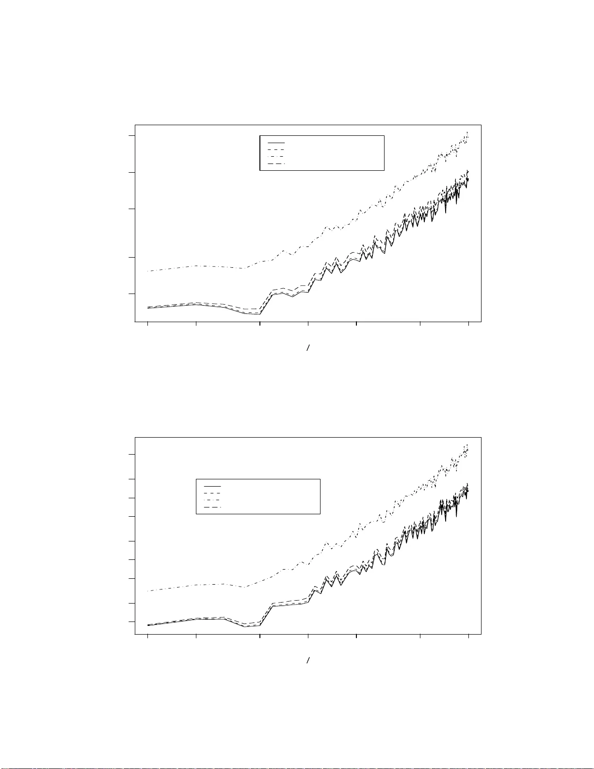
Analytic Bias Reduction for k –Sample F unction als 1 b y Christopher S. Withers Applied Mathematics Group Industr ial Researc h Limited Lo w er Hu tt, NEW Z EALAND Saralees Nadara jah Sc ho ol of Mathematics Univ ersit y of Manchester Manc hester M13 9PL, UK Abstract: W e giv e analytic metho ds for nonparametric bias redu ction that remo v e the need for computationally in tensiv e metho ds lik e the b o otstrap and the jackknife. W e call an estimate p th or d er if its bias has magnitude n − p 0 as n 0 → ∞ , where n 0 is the sample size (or the minim um sample size if the estimate is a fu n ction of more than one sample). Most estimates are only firs t order and require O ( N ) calculat ions, w here N is th e total sample size. The usual b o otstrap and jac kknife estimates are second order bu t they are computationally int ensiv e, requiring O ( N 2 ) calculatio ns for on e sample. By con trast Jaec k el ’s infinitesimal jac kknife is an analytic second order one sample estimate requirin g only O ( N ) calculat ions. When p th order b o otstrap and jac kknife estimates are a v ailable, they require O ( N p ) ca lculations, and so b ecome ev en more computationally in tens ive if one chooses p > 2. F or general p w e pro vide analytic p th order nonparametric estimates that r equire only O ( N ) calculatio ns. Our estimates are give n in terms of the v on Mises deriv ativ es of the fu nctional b eing estimated, ev aluated at the emp irical d istribution. F or pr o ducts of moments an unbiased estimate exists: our form f or this “p olyk ay” is m u c h simpler than the usual f orm in terms of p ow er sums . 1 In tro duction and Su mmary Let T ( F ) b e any smo oth functional of one or more u nkno wn distr ibutions F based on random samples from them. Bia s r eduction of estimates of T ( F ), say T ( b F ), has b een a su b ject of con- siderable interest. T rad itionally bias reduction has b een based on w ell kno w n resampling metho ds lik e b o otstrapping and jac kknifing in n onparametric settings, see Efron (1982). Ho wev er, these metho ds ma y not b e effectiv e in complex situations when the sampling d istribution of the statistic c h anges to o abruptly with the parameter, or when this distribution is v ery ske w ed and has hea vy tails. Also the robustness prop erties of F ma y not b e preserv ed for T ( F ) for all T ( · ). Recen tly , v arious analytical m etho ds ha ve b een dev elop ed for bias reduction in parametric settings. Withers (1987) d evelo p ed metho d s for bias redu ction based on T a ylor series expansions. 1 AMS 1991 Subje ct Classific ation: Primary 62G03; Secondary 62G20, 62G30. Key Wor ds and Phr ases: Bias reduction; k –samples; Nonparametric; U –statistics; Unbiased estimate; V on Mises deriv atives. 1 Sen (1988) established asymptotic normalit y of √ n { T ( b F ) − T ( F ) } as n → ∞ und er suitable regularit y cond itions. C abrera and F ernh olz (1999, 2004) d efined a tar get estimator : for a giv en T and a parametric family of distr ib utions it is defined b y setting the exp ected v alue of the statistic equal to the observed v alue. Cabrera and F ernholz (1999, 2004 ) established und er suitable regularit y conditions that the target estimator has smaller bias and mean squared error th an the original estimator. See also F ernholz (2001). This pap er pro vides th e fir st analytical metho d s for nonparametric bias reduction. W e give three analytic metho ds for obtaining unbiased estimates ( UE s ) of an y sm o oth fu nctional T ( F ). These UEs are in general infinite series which in p ractice n eed to b e tr u ncated. Let u s d efine a p th or der estimate as one with bias O ( n − p 0 ) as n 0 → ∞ , where n 0 is the minim um samp le size. Our truncated p th order estimates require only O ( N ) computations, where N is th e total sample size. By con trast computer intensiv e metho ds, like the p th order b o otstrap and jac kknife estimates r equire O (( n 1 · · · n k ) p ) calculations. Put another wa y , for fixed p , the compu tational efficiency of our analytic p th order estimate relativ e to the p th order b o otstrap or jac kknife estimate is O ( n p − 1 0 ). So, our truncated estimates remo v e the need for these computationally intensiv e metho ds of nonparametric bias reduction. The do wn side is that the details m ust b e w ork ed out for eac h non p arametric fu nctional of int erest. This in v olves calculating the von Mises or functional deriv ativ es of the fu nctional up to order 2 p − 2. When vo n Mises (1947) in tro duced th ese d eriv ativ es, he did not d efine them u niquely , nor did he give a metho d to obtain higher deriv ativ es. This w as rectified in Wi thers (1983): the second deriv ativ e is not the deriv ativ e of the first d eriv ativ e, bu t requires a ‘correction’ term. v on Mises did give a metho d for calculating the fir st deriv ativ e, also kno wn as the influenc e function and this is well kno w n and widely used. v on Mises’ expansion for sa y T ( b F ) ab out T ( F ) w as extended to f unctionals of more than one distribution in Withers (1988). This in tro d uced f or the first time the partial v on Mises d eriv ativ es and sh o wed h o w to calculate them. Supp ose w e observ e k indep endent random samples of sizes n = ( n 1 , . . . , n k ) from k unknown distributions F = ( F 1 , . . . , F k ) on R s 1 , . . . , R s k , where R is the r eal line. Let b F = ( b F 1 , . . . , b F k ) b e their k empirical (or sample) distribu tions. W e shall giv e three p th order estimates of any smo oth functional T ( F ) in terms of the deriv ativ es of T ( F ) up to order 2 p − 2 ev aluated at b F . As noted we deriv e these p th ord er estimates fr om three forms of UE f or T ( F ). These are all infin ite series unless T ( F ) is a p olynomial in F , (for example, a p olynomial in the moments of F 1 , . . . , F k ). T runcation of these series y ields three f orms of estimates of T ( F ) of bias O ( n − p 0 ), where n 0 = min k i =1 n i and p ≥ 1 is any sp ecified integ er. W e call these th ree forms of estimates the S, T and V estimates. F or p = 2, all three f orm s of estimates ha v e k + 1 terms. But for p > 2 the S estimate is the b est choic e, r equiring few er terms than the T estimate or the V estima te: see Section 5. The T estimate is its p o w er series equiv alent. The V estimate is an in termediate form for arrivin g at th e S estimate. If T ( F ) is a pr o duct of moments or cumulan ts, then an un biased estimate of it exists, and is giv en by our S estimate with the appropr iate c h oice of p . Sp ecial cases include the UEs of the cum ulan ts of Fisher (1929 ), th e UEs of the cen tral momen ts of James (1958 ), an d the p olyk a ys of Wish art (1952) giv en in terms of the p o w er su ms via tables of the symmetric p olynomials: see Stuart and Ord (1987 , Section 12.22). Ou r S estimate give s these p olyk a ys in terms of the samp le cen tr al momen ts and so is muc h more compact and a v oids the n eed f or these tables. F or p = 2 and k = 1 the relation of our S estimate to the infinitesimal jackknife of J aec kel (1972 ) is giv en in App endix A. Jaec k el ga v e formulas for second order estimat es in terms of th e 2 deriv ativ es with resp ect to the we igh ts of T ( b F ), where b F is no w the weig hte d empirical distribu tion. His f orm ulas are equiv alen t to our second order one sample S and T estimates. Our formula s are giv en in terms of the second deriv ativ es of T ( F ). F or the case of one sample problems (functionals of only one d istribution function), the S and T estimates giv en h ere we re obtained by a muc h m ore lab orious approac h in Withers (1994a) s tarting with an expansion for E T ( b F ) based on a generalised delta metho d ; results were giv en up to p = 4. (This also con tains more examples.) Here these results are extended to p = 6 for the general k - sample p roblem. The present metho d uses U -statistics and so b ypasses the need in Withers (1994a) to differen tiate f u nctionals of deriv ativ es. A t th is p oint w e giv e four simple one sample examples dealt with in S ection 6: • F or univ ariate data, a s econd ord er estimate of the stand ard deviation T ( F ) = σ is T ( b F ) { 1 + m − 1 s 1 ( b F ) } , where m = n or n − 1, s 1 ( F ) = ( β 4 + 3) / 8 and β 4 is the k u rtosis, that is the standardised fourth cen tral momen t. • F or univ ariate data, a second order estimate of T ( F ) = µ /σ is T ( b F ) + n − 1 S 1 ( b F ), where S 1 ( F ) = − β 3 / 2 − T ( F )(3 β 4 + 1) / 8 and β 3 is the ske wness, that is th e standard ised third cen tr al momen t. • F or biv ariate data a second ord er estimate of th e ratio of marginal means T ( F ) = µ 1 /µ 2 , is ( X 1 /X 2 ) { 1 + n − 1 [ X 1 X 2 / ( X 1 X 2 ) − X 2 2 /X 2 2 ] } . (The usual r atio estimate T ( b F ) = X 1 /X 2 has bias O ( n − 1 ).) • F or multiv ariate data, w e giv e a second ord er estimate of T ( F ) = ( α ′ µ ) q , w h ere µ is th e mean v ector and α is any give n v ector of the same d imension, is ( α ′ b µ ) q { 1 −  q 2  ( α ′ b µ ) − 2 α ′ b V α/ ( n − 1) } , where b µ is the sample mean, and b V is the sample co v ariance. Applications to sk ewness and kurtosis h a ve already b een giv en in Withers (1994b). A k -sample univ ariate example is given by interpreting µ i in the last example as the mean of the i th d istribution sampled, b µ i as the mean of the i th samp le, an d replacing α ′ b V α/ ( n − 1) by P k i =1 α 2 i b v i / ( n i − 1), where b v i is the i th sample v ariance. All these examples allo w for a p ossible initial transformation of the d ata X → h ( X ) sa y . The th ree analytic metho ds for obtaining UEs are as follo ws. T h e simp lest UE for T ( F ) has the S estimate ∞ X i 1 ,...,i k =0 S i 1 ··· i k ( b F ) / { ( n 1 − 1) i 1 · · · ( n k − 1) i k } , (1.1) where ( m ) i = m ( m − 1) · · · ( m − i + 1) = m ! / ( m − i )!. Clearly this can b e transformed if desired to the T estimate ∞ X i 1 ,...,i k =0 T i 1 ··· i k ( b F ) n − i 1 1 · · · n − i k k . (1.2) 3 The co efficien ts S i 1 ··· i k ( F ) and T i 1 ··· i k ( F ) are f u nctions of the partial vo n Mises d eriv ativ es of T ( F ) of order up to (2 i 1 , . . . , 2 i k ). The third form of UE for T ( F ) has the V estimate ∞ X r 1 ,...,r k =0 b V r 1 ··· r k / ( r 1 ! · · · r k !) , (1.3) where V r 1 ··· r k is determined by th e partial deriv ativ es of T ( F ) of order ( r 1 , . . . , r k ). If T ( F ) is a p olynomial in F (suc h as a p olynomial in the momen ts and cumulan ts of F ), then the S an d V forms of the UE reduce to finite sums. In S ection 2 w e deriv e the V estima te (1.3) and its m ultiv ariate analog ue using U -statistics and tables of the symmetric p olynomials. Section 3 d eriv es from it the S estimate (1.1). Section 4 deriv es the T estimate (1.2). The n um b er of terms required for these estimates and the b o otstrap estimate are compared in Section 5. Finally , Section 6 illustrates the three estimates using v arious examples, including the four listed ab o v e. W e sho w in particular that our estimat es consisten tly outp erform th ose due to Sen (1988) and C ab r era and F ern holz (1999 , 2004) . Comp u ter programs in MAPLE for the im p lemen tation of the V , S and T estimates for any p and k are giv en in App endix B. W e shall often use b old to denote an integ er vect or, for example, n n n for ( n 1 , n 2 , . . . , n k ), and 1 1 1 for (1 , . . . , 1). Similarly , w e write r ! r ! r ! = r 1 ! · · · r k ! and ( m ) i ( m ) i ( m ) i = ( m 1 ) i 1 · · · ( m k ) i k . With this notation, (1.1)–(1.3) b ecome ∞ X i i i = 0 0 0 S i i i ( b F ) / ( n n n − 1 1 1) i i i , ∞ X i i i = 0 0 0 T i i i ( b F ) / n n n − i i i , ∞ ∞ ∞ X r r r = 0 0 0 b V r r r / r r r ! . W e show that the tru ncated forms S np np np ( b F ) = p p p − 1 1 1 X i i i = 0 0 0 S i i i ( b F ) / ( n n n − 1 1 1) i i i , T np np np ( b F ) = p p p − 1 1 1 X i i i = 0 0 0 T i i i ( b F ) / n n n − i i i , V np np np ( b F ) = 2 p p p − 2 2 2 X r r r =0 0 0 b V r r r / r r r ! , all h a v e bias O ( n − p 1 1 + · · · + n − p k k ) as n n n → ∞ ∞ ∞ . 2 The V F orm of Un b iased Estimate 2.1 One Sample Let u s first consider the case of one d istribution F on R s and one sample X 1 , . . . , X n . F or G an y distribution on R s the von Mises-T aylo r expansion of T ( F ) ab ou t T ( G ) is T ( F ) = ∞ X r =0 V r ( F , G ) /r ! , (2.1) where V 0 ( F , G ) = T ( G ) and V r ( F , G ) = R · · · R T G ( x 1 · · · x r ) dF ( x 1 ) · · · dF ( x r ) for r ≥ 1, and T G ( x 1 · · · x r ) is the r th ord er (vo n Mises) d eriv ativ e of T ( G ), un iquely defined b y (2.1) sub j ect to th e constrain ts that T G ( x 1 · · · x r ) is not altered by p ermuting x 1 , . . . , x r , and R T G ( x 1 · · · x r ) dG ( x 1 ) = 0. The fi rst deriv ative or influenc e function of T ( G ) is just T G ( x ) = lim ǫ → 0 ( T ( G ǫ ) − T ( G )) /ǫ , where G ǫ ( y ) = (1 − ǫ ) G ( y ) + ǫI ( y ≤ x ) and I ( A ) is 1 or 0 for A true or false. A simple metho d of ob taining 4 T G ( x 1 · · · x r ) from T G ( x 1 · · · x r − 1 ) w as giv en in Withers (1983). F or example, S ( G ) = T G ( x ) h as deriv ativ e S G ( y ) = T G ( x, y ) − T G ( y ) so this giv es th e second deriv ativ e of T ( G ) in terms of its first deriv ativ e. Similarly , S ( G ) = T G ( x, y ) has deriv ativ e S G ( z ) = T G ( x, y , z ) − T G ( z , y ) − T G ( x, z ) so this giv es the third deriv ativ e. T he analogous f orm ula holds f or the d eriv ativ e of the general r th order deriv ativ e, with r ‘correction’ terms su btracted. F or fixed G an UE of V r ( F , G ) is the U -statisti c V n r ( b F , G ) = X r T G ( X i 1 · · · X i r ) / ( n ) r , (2.2) where P r sums ov er all ( n ) r p ermutatio ns of distinct i 1 , . . . , i r in 1 , . . . , n . S o, nV n 1 ( b F , G ) = n X i =1 T G ( X i ) = n Z T G ( x ) d b F ( x ) , ( n ) 2 V n 2 ( b F , G ) = n X i 6 = j T G ( X i , X j ) = ( n X i,j =1 − n X i = j =1 ) T G ( X i , X j ) = n 2 Z Z T G ( x 1 , x 2 ) d b F ( x 1 ) d b F ( x 2 ) − n Z T G ( x 2 1 ) d b F ( x 1 ) , where T G ( x 2 1 ) = T G ( x 1 , x 1 ), and so on. Note that V n r ( b F , G ) can b e written do wn usin g the tables of the symmetric p olynomials in Stuart and Or d (1987, App endix T able 10, page 554) for r ≤ 6 and David and Kend all (1949) for r ≤ 12. The last col umn of these tables expresses th e symmetric p olynomials [1 r ] = P r x i 1 · · · x i r , where P r sums o ver d istinct i 1 , . . . , i r in 1 , . . . , n s ay , in terms of the p o wer sum functions ( j ) = P n i =1 x j i for 1 ≤ j ≤ r . F or example, [1 4 ] = − 6(4) + 8(31) + 3(2 2 ) − 6(21 2 ) + (1 4 ), wh ere f or π = ( π 1 , . . . , π m ), ( π ) = ( π 1 ) · · · ( π m ). In general [1 r ] = r X π ( π ) c ( π ) , (2.3) where P r π sums o ver all partitions π of r , and the n umerical co efficients c ( π ) are pro vided in the last column of th e tables. The MAPLE pro cedu re s ymmp oly(...) in App endix B exp resses a giv en n um b er of symmetric p olynomials in terms of p o w er sum fu nctions. Ho wev er, the r elation (2.3 ) remains true if [1 r ] is redefi n ed as P r t ( x i 1 , . . . , x i r ) an d ( π ) = ( π 1 · · · π m ) is redefined as P n i 1 =1 · · · P n i m =1 t ( x π 1 i 1 , . . . , x π m i m ), w h ere x π 1 1 denotes π 1 argumen ts equal to x 1 , n ot a p o w er, and t is an arbitrary symmetric p olynomial of r v ariables. In p articular taking x i ≡ X i and t ≡ T G , [1 r ] = ( n ) r V n r ( b F , G ), and ( π ) = T b F G [ π ] n m ( π ) , where m = m ( π ) is the num b er of elemen ts in π , and T b F G [ π ] = Z · · · Z T G ( x π 1 1 · · · x π m m ) d b F ( x 1 ) · · · d b F ( x m ) . (2.4) So, (2.3) can b e wr itten V n r ( b F , G ) = ( n ) − 1 r r X π c ( π ) T b F G [ π ] n m ( π ) , 5 and an UE of T ( F ) is P ∞ r =0 V n r ( b F , G ) /r !. Since G is arbitrary we ma y no w tak e G = b F and s et b V r = V n r ( b F , b F ), b T [ π ] = T b F b F [ π ], T [ π ] = T F F [ π ]. F or example, f or second order estimates we shall need b T [2] = R T b F ( x, x ) d b F ( x ). Our expression ab o ve for LHS (2.2) at G = b F n o w yields the follo wing V form of UE for T ( F ): ∞ X r =0 b V r /r ! , (2.5) where b V r = ( n ) − 1 r X ∼ r π c ( π ) b T [ π ] n m ( π ) , (2.6) and P ∼ r π is P r π excluding partitions con taining 1 b ecause of the constrain t R T b F ( x 1 · · · x r ) d b F ( x 1 ) = 0. The first few V r are b V 0 = T ( b F ) , b V 1 = 0 , b V 2 = − ( n − 1) − 1 b T [2] , b V 3 = 2( n − 1) − 1 2 b T [3] , b V 4 = ( n − 1) − 1 3 {− 6 b T [4] + 3 b T [2 2 ] n } , b V 5 = 2( n − 1) − 1 4 { 24 b T [5] − 20 b T [32] n } , b V 6 = ( n − 1) − 1 5 {− 120 b T [6] + 90 b T [42] n + 40 b T [3 2 ] n − 15 b T [2 3 ] n 2 } . Using the O p ( . ) notation of Mann and W ald (1943), since b V 2 r − 1 and b V 2 r are O p ( n − r ), the UE (2.5) is V n :2 p − 2 ( b F ) + O p ( n − p ), wh ere V n : j ( b F ) = j X r =0 b V r /r ! . Note that V n :2 p − 2 ( b F ) estimates T ( F ) w ith bias O ( n − p ): V n :2 ( b F ) = T ( b F ) − ( n − 1) − 1 b T [2] / 2 has bias O ( n − 2 ), V n :4 ( b F ) = V n :2 ( b F ) + ( n − 1) − 1 2 b T [3] / 3 + ( n − 1) − 1 3 ( − 6 b T [4] + 3 b T [2 2 ] n ) / 24 has bias O ( n − 3 ), and so on. The MAPLE pr o cedures Vestsum(.. .) and Ve st(...) in App endix B calculate (2. 6) f or an y r an d hence V n :2 p − 2 for an y p , so estimates of bias of an y order can b e obtained. If T ( F ) is a p olynomial in F of degree p , f or example, µ p ( F ), κ p ( F ) or µ ( F ) p then T G ( x 1 · · · x r ) = 0 for r > p so that V np ( b F ) is an UE. 2.2 More than One Sample No w consider the case of k ≥ 1 distributions, with k samples { X 1 j , . . . , X n j j } , 1 ≤ j ≤ k . The von Mises–T a ylor expansion of T ( F ) ab out T ( G ) for G = ( G 1 , . . . , G k ) d istr ibutions on R s 1 , . . . , R s k is T ( F ) = ∞ X r 1 =0 · · · ∞ X r k =0 V r 1 ··· r k ( F , G ) / ( r 1 ! · · · r k !) = ∞ ∞ ∞ X r r r = 0 0 0 V r r r ( F , G ) / r r r ! , (2.7) where V r r r ( F , G ) = Z · · · Z T G  1 1 · · · 1 · · · k k · · · k x 1 x 2 · · · x r 1 · · · z 1 z 2 · · · z r k  dF 1 ( x 1 ) · · · dF 1 ( x r 1 ) · · · dF 1 ( z 1 ) · · · dF k ( z r k ) 6 and T G  a 1 · · · a r x 1 · · · x r  is the p artial (v on Mises) deriv ativ e, defi n ed for a 1 , . . . , a r in 1 , . . . , k and x i in R s a i . These were in tro duced in Withers (1988). Th ey are determined uniquely by (2.7) and the t wo constrain ts T G  a 1 · · · a r x 1 · · · x r  is n ot altered by p ermuting columns, and Z T G  a 1 · · · a r x 1 · · · x r  dF G a 1 ( x 1 ) = 0 . In practice they are determined by adapting the rules giv en ab o v e for the one distribu tion d eriv a- tiv es, namely: T G  a x  is j u st S G a ( x ) for S ( G a ) = T ( G ), U ( G b ) = T G  a x  has deriv ativ e U G b ( y ) = T G  a b x y  − T G  a x  and similarly for th e der iv ativ e of the general deriv ative . The term V 0 0 0 ( F , G ) is in terp reted as T ( G ). F or more d etails and examples see Wit hers (19 88, 1994a ). F or a giv en G , an UE of V r r r ( F , G ) is V n n n r r r ( b F , G ) = X r 1 ··· r k T G  1 · · · 1 · · · k · · · k X i 1 1 · · · X i r 1 1 · · · X j 1 k · · · X j r k k  / ( n n n ) r r r , where P r 1 ··· r k sums ov er all ( n 1 ) r 1 p ermutatio ns of distinct i 1 , . . . , i r 1 in { 1 , . . . , n 1 } , . . . and all ( n k ) r k p ermutatio ns of distinct j 1 , . . . , j r k in { 1 , . . . , n k } . So, ∞ ∞ ∞ X r r r = 0 0 0 V n r r r ( b F , G ) / r r r ! is an UE of T ( F ). T aking G = b F , ∞ ∞ ∞ X r r r = 0 0 0 b V r r r / r ! r ! r ! is a UE of T ( F ), where b V r r r = V n n n r r r ( b F , b F ). F or i 1 , . . . , i k in { 0 , 1 } , b V 2 r − i r − i r − i is O p ( n − r 1 1 · · · n − r k k ). So, V n n n :2 p p p − 2 2 2 ( b F ) estimates T ( F ) with bias O ( n − p 1 1 + · · · + n − p k k ) = O ( n − p 0 0 ), where V n n n : j j j ( b F ) = j j j X r r r = 0 0 0 b V r r r / r r r ! , n 0 = min 1 ≤ i ≤ k n i , p 0 = min 1 ≤ i ≤ k p i . Ho wev er for p 0 > 1, an estimate of T ( F ) of bias O ( n − p 0 0 ) with fewer terms than V n n n : 2 2 2 p 0 − 2 2 2 is V n n np 0 ( b F ) = 2 p 0 − 2 X r 0 =0 b V r 0 /r 0 ! , (2.8) where b V r 0 = r 0 ! X r 1 + ··· + r k = r 0 b V r r r / r r r ! . 7 If T ( F ) is a p olynomial of degree p 1 in F 1 , . . . , p k in F k , then the UE reduces to the finite sum V n n n : p p p ( b F ), conta ining ( p 1 + 1) · · · ( p k + 1) terms . This is b ecause b V r r r = 0 if r 1 > p 1 or · · · or r k > p k . Set T F ( i r j s · · · ) = Z Z · · · T F  i r j s · · · x r y s  dF j ( x ) dF j ( y ) · · · , where the first column in th e integ rand stands for r rep eated columns of  i x  , and similarly for the other columns. Set T F G [ π 1 , . . . , π k ] = T F G (1 π 11 · · · 1 π m 1 1 · · · 1 π 1 k · · · 1 π m k k ) for π 1 = ( π 11 · · · π m 1 1 ) , . . . , π k = ( π 1 k · · · π m k k ). (So, m k is the length of th e vec tor π k .) Set b T [ π 1 · · · π k ] = T b F b F [ π 1 · · · π k ] , b T ( i r j s · · · ) = T b F b F ( i r j s · · · ) , T ( i r j s · · · ) = T F F ( i r j s · · · ) . Analogous to (2.5) we h av e b V r r r = ( n n n ) − 1 r r r ∼ r 1 X π 1 · · · ∼ r k X π k c ( π 1 ) · · · c ( π k ) b T [ π 1 , . . . , π k ] n m ( π 1 ) 1 · · · n m ( π k ) k . (2.9) The MAPLE pro cedures V estsum(...) and V est(...) in App en dix B calculate (2.9) for an y r r r and hence (2.8) for an y p 0 , so estimates of bias of an y order can b e obtained. Let e i b e the i th un it v ector in R k . Then the first six b V r 0 of (2.8) are b V 0 = T ( b F ) , b V 1 = k X i =1 b V e i = 0 , b V 2 = k X i =1 b V 2 e i = − k X i =1 T b F ( i 2 ) / ( n i − 1) , since b V e i + e j = 0 for i 6 = j , b V 3 = k X i =1 b V 3 e i = 2 k X i =1 b T ( i 3 ) / ( n i − 1) 2 , b V 4 = k X i =1 b V 4 e i +  4 2  X 1 ≤ i 1. (Note that Hall’s (1.35) should hav e a factor ( − 1) i +1 inserted.) If one allo ws p to increase and coun ts the n um b er of terms needed, then as shown by T able 5.1, S n n np ( b F ) requires increasingly few er terms than do V n n np ( b F ) and T n n np ( b F ). [T ables 5.1–5.3 ab out here.] The n umber of terms in an expr ession of the form P 1 ≤ i 1 < ··· 1, S n 0 p ( b F ) and T n 0 p ( b F ) in Withers (1994a) differ from S n n np ( b F ) and T n n np ( b F ) giv en here. All ha ve bias O ( n − p 0 ), b ut the forms giv en h ere are more n atural. In th is section we go o v er some of the examples of Withers (199 4a) to obtain S estima tes, S n n np ( b F ), of bias O ( n − p 0 ) up to p = 7. Recall that for k = 1 this is giv en by S np ( b F ) = p − 1 X i =0 S i ( b F ) / ( n − 1) i (6.1) 14 for S i ( F ) of (3.4 )–(3.9), and for k > 1 b y (3. 10)–(3.17). W e b egin with t w o p roblems estimating a general fun ction of the means of the distrib utions after initial giv en transf ormations of the data. When this function of the means is a p olynomial of to tal degree p 0 w e sh o w that f or b oth pr ob- lems S np 0 ( b F ) is an UE. W e then giv e examples estimating functions of cen tral moments. W e use the co n v en tion that rep eated indices are sum med ov er their range. F or example, in (6.2) b elo w, i 1 · · · j 1 · · · are implicitly summed o ver 1 , . . . , t . Example 6.1 k = 1 , T ( F ) = g ( µ ), wh ere µ = R hdF = E h ( X ) for X ∼ F , where h : R s → R t and g : R t → R are giv en f unctions. Assume that the partial deriv ativ es of g ( µ ) are finite: g j 1 ··· j r = ∂ j 1 · · · ∂ j r g ( µ ), where ∂ j = ∂ /∂ µ j . Then the general deriv ativ e of T ( F ) is T F ( x 1 · · · x r ) = g j 1 ··· j r µ j 1 x 1 · · · µ j r x r , where µ j x = µ j F ( x ) = h j ( x ) − µ j . So, T [ π ] = g i 1 ··· i π 1 j 1 ··· j π 2 ··· µ [ i 1 · · · i π 1 ] µ [ j 1 · · · j π 2 ] · · · , (6.2) where µ [ i 1 i 2 · · · ] = R ( h ( x ) − µ ) i 1 ( h ( x ) − µ ) i 2 · · · dF ( x ), the joint ce n tral moment of h ( X ). Sub- stituting in to (3.4)–(3.9) giv es S i ( F ) for i ≤ 6 so (6.1) giv es an estimate of bias O ( n − 7 ). No w for i ≥ 1 , S i ( F ) has the form P 2 i r = i +1 g j 1 ··· j r c ij 1 ··· j r . So, if g ( µ ) is a p olynomial of degree p p p in µ (that is of d egree p i in µ i for 1 ≤ i ≤ t ), th en su mmation m ay b e r estricted to j 1 , . . . , j r with P r i =1 I ( j i = a ) ≤ p a for 1 ≤ a ≤ t , and S i ( F ) = 0 for i ≥ | p p p | = p 1 + · · · + p t so S n, | p p p | ( b F ) is an UE. So, (6.1), (3.4)–(3 .9 ) give s an UE for all p olynomials g ( µ ) of total degree sev en or less.  Example 6 .1.1 g ( µ ) = N q , where N = α ′ µ for some t -vec tor α . If π = ( π 1 , . . . , π m ) and r = π 1 + · · · + π m then T [ π ] = ( q ) r N q α ( π 1 ) · · · α ( π m ), where α ( i ) = N − i α j 1 · · · α j i µ [ j 1 · · · j i ]. F or example, α (2) = N − 2 α ′ b V α , where V = cov ar { h ( X ) } . So, a second order estimate of ( α ′ µ ) q is ( α ′ b µ ) q { 1 −  q 2  ( α ′ b µ ) − 2 α ′ b V α/ ( n − 1) } , wh ere b µ, b V are the sample estimates of µ = h ( X ), and V . [Figures 6.1 and 6.2 ab out h er e.] No w supp ose q = t = 2, α = ( α 1 , 1 − α 1 ) and V = I 2 . The second order estimate redu ces to { α 1 c µ 1 + (1 − α 1 ) c µ 2 } 2 − { α 2 1 + (1 − α 1 ) 2 } / ( n − 1). If h ( X ) is biv ariate normal with un it means and the giv en V then th e target estimator (Cabrera and F ern h olz, 1999, 2004) of ( α ′ µ ) 2 is { α 1 c µ 1 + (1 − α 1 ) c µ 2 } 2 − { α 2 1 + (1 − α 1 ) 2 } /n . Sen (1988)’s asymptotic norm alit y pr o vid es b ω , the maxi- m um likel iho o d estimate of ω giv en ( α ′ b µ ) 2 ∼ N ( ω , (3 /n ) { α 2 1 + (1 − α 1 ) 2 } 2 + (4 ω /n ) { α 2 1 + (1 − α 1 ) 2 } ). Figures 6.1 and 6.2 compare the p erformance of these three estimates an d those obtained by b o ot- strapping and jac kknifing. Our estimate has the low est absolute bias and the lo west mean squared error. T h e estimates due to C abrera and F ernholz (1999 , 200 4) are so close to ours that they are indistinguishable. Next supp ose t = α = 1 so T ( F ) = µ q , µ = E h ( X ), α ( i ) = µ − i µ i , µ i = E ( h ( X ) − µ ) i and T [ π ] = ( q ) r µ q − r µ π 1 ··· µ π m . Also for i ≥ 1, S i ( F ) = 2 i X r = i +1 ( q ) r µ q − r S ir , (6.3) where S 12 = − µ 2 / 2, S 23 = µ 3 / 3, S 24 = µ 2 2 / 8, S 34 = − µ 4 + 3 µ 2 2 / 8, S 35 = − µ 3 µ 2 / 6 , S 36 = − µ 3 2 / 48, S 45 = µ 5 / 5 − 2 µ 3 µ 2 / 3, S 46 = − 3 µ 3 2 / 16 + µ 4 µ 2 / 8 + µ 2 3 / 18, S 47 = µ 3 µ 2 2 / 48, S 48 = µ 4 2 / 384, S 56 = − µ 6 / 6 + 5 µ 4 µ 2 / 8 + 5 µ 2 3 / 18, S 57 = − µ 5 µ 2 / 10 − µ 4 µ 3 / 12, S 58 = 3 µ 2 4 µ 2 2 / 32 − µ 2 3 µ 2 / 36, S 59 = − µ 3 µ 3 2 / 144, S 5 , 10 = − µ 5 2 / 3840 , S 67 = µ 7 / 7 − 3 µ 5 µ 2 / 5 − µ 4 µ 3 / 2 + µ 3 µ 2 2 / 140, S 68 = 127 µ 4 2 / 64 − 13 µ 4 µ 2 2 / 32 − 327 µ 2 3 µ 2 / 100 + µ 6 µ 2 / 12 + µ 5 µ 3 / 15 + µ 2 4 / 32, S 69 = − 7 µ 3 µ 3 2 / 48 + µ 5 µ 2 2 / 40 + µ 4 µ 3 µ 2 / 24 + µ 3 3 / 324, S 6 , 10 = − µ 5 2 / 160 + µ 2 3 µ 2 2 / 144 + µ 4 µ 3 2 / 192, S 6 , 11 = µ 3 µ 4 2 / 1152 and S 6 , 12 = µ 6 2 / 4608 0. T his 15 giv es S i ( F ) for i ≤ 6 and so S n 7 ( b F ) of bias O ( n − 7 ). If q is a p ositiv e in teger, then S i ( F ) = 0 f or i ≥ q so S nq ( b F ) of (6.1 ), (6.3) is an UE of µ q . F or example, an UE of µ 4 is giv en b y (6.1) with S 1 ( F ) = − 6 µ 2 µ 2 , S 2 ( F ) = 8 µµ 3 + 3 µ 2 2 , S 3 ( F ) = − 6 µ 4 + 9 µ 2 2 . Th is result ma y b e chec k ed by solving the system of sev en equations giv en b y Wishart (1952, page 5). Alternativ ely one ma y follo w the metho d of Stu art and Ord (1987 , Sectio n 12.22 ) us in g their tables of the symmetric p olynomials. F or example, one obtains the UE T n ( b F ) for µ 4 , where ( n − 1) 3 T n ( F ) = ( n 3 − 8 n 2 + 23 n − 30) m 4 − n ( n 2 − 7 n + 4) m 3 m 1 − n ( n 2 − 6 n + 6) m 2 2 + n 2 ( n − 9) m 2 m 2 1 + n 3 m 4 1 , where m i = E X i . Clearly our metho d giv es the simpler form.  Example 6.1.2 t = 2, g ( µ ) = µ 1 µ − 1 2 . Then g 12 j = ( − 1) j j ! µ − j − 1 2 = a j sa y , g 2 j = µ 1 a j , and g π = 0 unless π is a p erm utation of 2 j or 12 j for some j . F or π = ( π 1 , π 2 , . . . ) set | π | = π 1 + π 2 + · · · and α [ π ] = µ [ π ] / ( µ π 1 µ π 2 · · · ) = E ( X π 1 /µ π 1 − 1)( X π 2 /µ π 2 − 1) · · · . Then T [ π ] = µ 1 µ − 1 2 ( − 1) | π | α [2 π 1 ] α [2 π 2 ] · · · {| π | ! − ( | π | − 1)! X i π i α [12 π i − 1 ] /α [2 π i ] } . So, S 1 ( F ) /T ( F ) = α [12] − α [22] = E X 1 X 2 / ( µ 1 µ 2 ) − E X 2 2 /µ 2 2 , S 2 ( F ) /T ( F ) = − 2 α [222] + 2 α [122] + 3 α [22] 2 − 3 α [12] α [22] , S 3 ( F ) /T ( F ) = 6 α [12 3 ] − 6 α [2 4 ] − 9 α [12] α [ 22] + 9 α [22 2 ] +20 α [2 3 ] α [2 2 ] − 12 α [12 2 ] α [2 2 ] − 8 α [2 3 ]) α [12] +15 α [12] α [ 22] 2 − 15 α [22] 3 , S 4 ( F ) /T ( F ) = 24 α [12 4 ] − 24 α [2 5 ] + 80 α [2 3 ] α [2 2 ] − 48 α [12 2 ] α [2 2 ] − 32 α [2 3 ] α [12] + 45 α [2 2 2 ]( α [12] − α [22]) +90 α [2 4 ] α [2 2 ] − 60 α [12 3 ] α [2 2 ] − 30 α [2 4 ] α [12] +40 α [2 3 ]( α [2 3 ] − α [12 2 ]) − 210 α [2 3 ] α [2 2 ] 2 + 90 α [12 2 ] α [2 2 ] 2 +120 α [2 3 ] α [12] α [2 2] + 105 α [22 ] 3 ( α [22] − α [12]) , S 5 ( F ) /T ( F ) = 120 α [12 5 ] − 120 α [2 6 ] + 150 α [2 4 ](3 α [22 ] − α [12]) − 300 α [12 3 ] α [2 2 ] + 200 α [2 3 ]( α [2 3 ] − α [12 2 ]) +72 α [2 5 ](7 α [2 3 ] − 3 α [12 3 ]) − 360 α [1 2 4 ] α [2 3 ] +60 α [2 4 ](7 α [2 3 ] − 3 α [12 2 ]) − 240 α [1 2 3 ] α [2 3 ] +1890 α [2 2 ] 3 ( α [22] − α [12]) + 630 α [2 4] α [22]( α [12] − 2 α [22]) +630 α [12 3 ] α [2 2 ] 2 + 210 α [2 3 ] 2 ( α [12] − 4 α [22 ]) − 630 α [12 2 ] α [2 3 ] α [22] + 945 α [2 2 ] 4 ( α [12] − α [22]) +840 α [2 2 ] 2 (3 α [2 3 ] α [2 2 ] − α [12 2 ] α [2 2 ] − 2 α [2 3 ] α [12]) , and similarly for S 6 ( F ). [Figures 6.3 and 6.4 ab out h er e.] It follo ws that a second order estimate of µ 1 /µ 2 is ( X 1 /X 2 ) { 1 + n − 1 [ X 1 X 2 / ( X 1 X 2 ) − X 2 2 / X 2 2 ] } , where X 1 and X 2 are the sample means for X 1 and X 2 , resp ectiv ely . I f X i , i = 1 , 2 are indep endent 16 exp onenti al rand om v ariables with means µ i , i = 1 , 2 then a target estimator (Cabrera and F ernholz, 1999, 2004) of µ 1 /µ 2 is (( n 2 − 1) /n 2 )( X 1 /X 2 ), wh ere n 2 denotes the sample size for X 2 . Sen (1988)’ s conditions f or asymptotic normalit y do n ot hold h ere. Figures 6.3 and 6.4 compare the p erformance of the tw o estimates and those obtained b y b o otstrapping an d j ackknifing. Our estimate again pro vides the lo w est absolute bias and the lo west mean sq u ared error, but the differences with resp ect to th e target estimator do n ot app ear to b e significant.  Example 6.2 T ( F ) = g ( µ ), where µ = ( µ 1 , . . . , µ k ), µ i = R h i dF i = E h i ( X i ) for X i ∼ F i , h i : R s i → R is a giv en fu nction, and g : R k → R is a giv en fu nction with finite partial deriv ativ es g j 1 ··· j r . Then T F  i 1 · · · i r x 1 · · · x r  = g i 1 ··· i r µ i 1 x 1 · · · µ i r x r , where µ ix = µ iF i ( x ) = h i ( x ) − µ i . So, T ( i a j b · · · ) = g i a j b ··· µ a [ i ] µ b [ j ] · · · , where µ a [ i ] = µ a ( h i ( X i )) = R ( h i ( x ) − µ i ) a dF i ( x ). An estimate of b ias O ( n − p 0 ) is S n n np ( b F ) = P p − 1 i =0 S n n n i ( b F ), where by (3.11)–(3.17), S n n n 0 ( F ) = g ( µ ) , S n n n 1 ( F ) = − (1 / 2) k X i =1 g i 2 µ 2 [ i ]( n i − 1) − 1 , S n n n 2 ( F ) = k X i =1 { g i 3 µ 3 [ i ] / 3 + g i 4 µ 2 [ i ] 2 / 8 } ( n i − 1) − 1 2 + X 1 ≤ ik) then for i from 1 to (j-k) do d[j-i]:= 0; for n from (j-i+1) to j do d[j-i]:= d[j-i]+d [n]*Amkr(j-i,n,r); od; d[j-i]:= -d[j-i]/ (Amkr(j-i,j-i,r)); od; tt:=d[k] ; end if; return(t t); end proc; #the followi ng procedur e is needed as part of the above cc (k, j, r) procedure Amkr := proc (m, k, r) sum(((-1 )**(l+k) )*stirling1(k,l)*binomial(l,m)*(1-r)**(l-m),l=m..k); end proc; #this procedure compute s the k (ndim) fold summation in equatio n (2.9) #here it is assumed implic itly that k=5 #but the proced ure can be applied for any k by making appropria te changes to #the five do-loops and the five statement s following it #this procedure require s as input: n[1],n[2], ...,n[k] ,r[1],r[2],...,r[k], #ndim=th e value of k,the output from symmpoly () and the T(.) function #in equation (2.4) the output from this procedur e is needed as input for #the Vest() and coeffic ients() procedures Vestsum := proc (ndim,n ::list,r ::list,e::list,T) local kk,pa,ss, i1,i2,i3, i4,i5,paa,bb,tt,kkk,j,nn,ttt,mmm; for kk from 1 to ndim do pa[kk]:= partitio n(r[kk]); od; ss:=0; for i1 from 1 to nops(pa[1 ]) do for i2 from 1 to nops(pa[2 ]) do for i3 from 1 to nops(pa[3 ]) do for i4 from 1 to nops(pa[4 ]) do for i5 from 1 to nops(pa[5 ]) do paa[1]:= pa[1][i1 ]; paa[2]:= pa[2][i2 ]; paa[3]:= pa[3][i3 ]; paa[4]:= pa[4][i4 ]; paa[5]:= pa[5][i5 ]; bb:=memb er(1,paa [1])=false; for kk from 2 to ndim do bb:=bb and member(1 ,paa[kk] )=false; od; 28 if (bb) then for kk from 1 to ndim do tt[kk]:= expand(e [r[kk]]); od; for kkk from 1 to ndim do for j from 1 to r[kkk] do nn:=0; for kk from 1 to nops(paa[ kkk]) do if (j=paa[kk k][kk]) then nn:=nn+1 end if; od; if (nn>0) then tt[kkk]: =coeff(t t[kkk],p[j],nn) end if; od; od; ttt:=1; for mmm from 1 to ndim do ttt:=ttt *tt[mmm] *(n[mmm])**(nops(paa[mmm])); od; ss:=ss+t tt*T([se q(paa[mm],mm=1..ndim)]); end if; od; od; od; od; od; ss:=expa nd(ss); return(s s); end proc; #this procedure compute s of the coefficie nts of the output from #with respect to powers of n[1],n[ 2],...,n [k] #It is assumed implicit ly that k is 5 #the procedu re can be applied to any k by changin g the number #of do loops and making other appropr iate changes #this procedure require s as input: n[1],n[2], ...,n[k] ,r[1],r[2],...,r[k] #and the output from Vestsum() #the output from this procedur e is needed as input for the Sest() #and Test() procedu res coeffici ents := proc(n: :list,r: :list,ss) local i1,i2,i3, i4,i5,sss ,A; A:=array (1..r[1] /2,1..r[2]/2,1..r[3]/2,1..r[4]/2,1..r[5]/2); for i1 from 1 to r[1]/2 do for i2 from 1 to r[2]/2 do for i3 from 1 to r[3]/2 do for i4 from 1 to r[4]/2 do for i5 from 1 to r[5]/2 do sss:=coe ff(ss,n[ 1],i1); sss:=coe ff(sss,n [2],i2); 29 sss:=coe ff(sss,n [3],i3); sss:=coe ff(sss,n [4],i4); sss:=coe ff(sss,n [5],i5); A[i1,i2, i3,i4,i5 ]:=sss; od; od; od; od; od; return(A ); end proc; #this procedure compute s V_r for the V estimate in Section 2 #this procedure require s as input: n[1],n[2], ...,n[k] ,r[1],r[2],...,r[k], #ndim=th e value of k,the output from symmpoly () and the T(.) function #in equation (2.4) Vest := proc(nd im,n::lis t,r::list,e::list,T) local ss,mm; ss:=Vest sum(ndim ,n,r,e,T); ss:=ss*( product( factorial(n[mm]-r[mm]),mm=1..ndim)); ss:=ss/( product( factorial(n[mm]),mm=1..ndim)); ss:=simp lify(ss) ; return(s s); end proc; #this procedure compute s V_r for the S estimate in Section 3 #It is assumed implicit ly that k is 5 #the procedu re can be applied to any k by changin g the number #of do loops and making other appropr iate changes #this procedure require s as input: n[1],n[2], ...,n[k] , #r[1],r[ 2],...,r [k] and the output from coeffic ients() Sest := proc(n: :list,r:: list,A::array) local i1,i2,i3, i4,i5,j1, j2,j3,j4,j5,tt,ttt,ss; ss:=0; for i1 from r[1]/2 to r[1]-1 do for i2 from r[2]/2 to r[2]-1 do for i3 from r[3]/2 to r[3]-1 do for i4 from r[4]/2 to r[4]-1 do for i5 from r[5]/2 to r[5]-1 do tt:=0; for j1 from r[1]-i1 -1 to r[1]/2-1 do for j2 from r[2]-i2 -1 to r[2]/2-1 do for j3 from r[3]-i3 -1 to r[3]/2-1 do for j4 from r[4]-i4 -1 to r[4]/2-1 do for j5 from r[5]-i5 -1 to r[5]/2-1 do ttt:=A[j 1+1,j2+1 ,j3+1,j4+1,j5+1]*cc(r[1]-i1-1,j1,r[1])*cc(r[2]-i2-1,j2,r[2]); 30 ttt:=ttt *cc(r[3] -i3-1,j3,r[3])*cc(r[4]-i4-1,j4,r[4])*cc(r[5]-i5-1,j5,r[5]); tt:=tt+t tt; od; od; od; od; od; tt:=tt*f actorial (n[1]-i1-1)*factorial(n[2]-i2-1)*factorial(n[3]-i3-1); tt:=tt*f actorial (n[4]-i4-1)*factorial(n[5]-i5-1); tt:=tt/( factoria l(n[1]-1)*factorial(n[2]-1)); tt:=tt/( factoria l(n[3]-1)*factorial(n[4]-1)*factorial(n[5]-1)); ss:=ss+t t; print(i1 ,i2,i3,i 4,i5,ss); od; od; od; od; od; ss:=simp lify(ss) ; return(s s); end proc; #this procedure compute s V_r for the T estimate in Section 4 #It is assumed implicit ly that k is 5 #the procedu re can be applied to any k (ndim) by changin g the number #of do loops and making other appropr iate changes #this procedure require s as input: n[1],n[2], ...,n[k] ,r[1],r[2],...,r[k], #ndim=th e value of k and the output from coeffici ents() Test := proc(nd im,n::lis t,r::list,A::array) local i1,i2,i3, i4,i5,j1, j2,j3,j4,j5,nn,tt,ttt,tttt,ss,a,kk; ss:=0; for i1 from r[1]/2 to r[1]-1 do for i2 from r[2]/2 to r[2]-1 do for i3 from r[3]/2 to r[3]-1 do for i4 from r[4]/2 to r[4]-1 do for i5 from r[5]/2 to r[5]-1 do tt:=0; for j1 from r[1]-i1 -1 to r[1]/2-1 do for j2 from r[2]-i2 -1 to r[2]/2-1 do for j3 from r[3]-i3 -1 to r[3]/2-1 do for j4 from r[4]-i4 -1 to r[4]/2-1 do for j5 from r[5]-i5 -1 to r[5]/2-1 do ttt:=A[j 1+1,j2+1 ,j3+1,j4+1,j5+1]*cc(r[1]-i1-1,j1,r[1])*cc(r[2]-i2-1,j2,r[2]); ttt:=ttt *cc(r[3] -i3-1,j3,r[3])*cc(r[4]-i4-1,j4,r[4])*cc(r[5]-i5-1,j5,r[5]); tt:=tt+t tt; od; od; 31 od; od; od; nn[1]:=i 1; nn[2]:=i 2; nn[3]:=i 3; nn[4]:=i 4; nn[5]:=i 5; ttt:=1; for kk from 1 to ndim do tttt:=0; for a from nn[kk] to 100 do tttt:=tt tt+(n[kk ])**(-a)*dalphai(a,nn[kk]); od; ttt:=ttt *tttt; od; ss:=ss+t t*ttt; print(i1 ,i2,i3,i 4,i5,ss); od; od; od; od; od; ss:=simp lify(ss) ; return(s s); end proc; 32 T able 5.1. Numb er of terms for estimates of bias O ( n − p ) for k = 1. p = 1 2 3 4 5 6 7 V n n np ( b F ) 1 2 5 11 22 42 77 S n n np ( b F ) 1 2 4 8 15 25 44 T n n np ( b F ) 1 2 5 11 21 · · T able 5.2. Numb er of terms for estimates of bias O ( n − p 0 ), where n 0 = min n i . p = 1 2 3 4 5 V n n np ( b F ) 1 k + 1 s 2 + 4 k + 1 s 3 + 8 s 2 + 10 k + 1 s 4 + 14 s 3 + 31 s 2 + 21 k + 1 = ( k 2 + 7 k + 2 ) / 2 = ( k 3 + 21 k 2 + 38 k + 6) / 6 = ( k 4 + 40 k 3 + 305 k 2 + 230 k + 2 4) / 24 S n n np ( b F ) 1 k + 1 s 2 + 3 k + 1 s 3 + 3 s 2 + 7 k + 1 s 4 + 9 s 3 + 15 s 2 + 14 k + 1 = ( k 2 + 5 k + 2 ) / 2 = ( k 3 + 6 k 2 + 35 k + 6) / 6 = ( k 4 + 30 k 3 + 143 k 2 + 234 k + 2 4) / 24 T n n np ( b F ) 1 k + 1 s 2 + 4 k + 1 s 3 + 7 s 2 + 10 k + 1 s 4 + 13 s 3 + 25 s 2 + 20 k + 1 = ( k 2 + 7 k + 2 ) / 2 = ( k 3 + 18 k 2 + 20 k + 6) / 6 = ( k 4 + 36 k 3 + 245 k + 2 70 k + 24) / 2 4 T able 5.3. Numb er of terms for estimates of bias O ( n − p ) for k = 2 and 3. k = 2 k = 3 p = 1 2 3 4 5 1 2 3 4 5 V n n np ( b F ) 1 3 10 29 74 1 4 16 56 171 S n n np ( b F ) 1 3 8 18 44 1 4 13 32 97 T n n np ( b F ) 1 3 10 28 66 1 4 16 53 149 33 0.0 0.2 0.4 0.6 0.8 1.0 0.0 0.2 0.4 0.6 0.8 1.0 α 1 Average Absolute Bias 0.0 0.2 0.4 0.6 0.8 1.0 0.0 0.2 0.4 0.6 0.8 1.0 0.0 0.2 0.4 0.6 0.8 1.0 0.0 0.2 0.4 0.6 0.8 1.0 0.0 0.2 0.4 0.6 0.8 1.0 0.0 0.2 0.4 0.6 0.8 1.0 0.0 0.2 0.4 0.6 0.8 1.0 0.0 0.2 0.4 0.6 0.8 1.0 Withers & Nadarajah Cabrera & Fernholz Sen Bootstrap Jackknife Figure 6.1. The a verag e abs olute bias of the estimator of { α 1 µ 1 + (1 − α 1 ) µ 2 } 2 when µ 1 and µ 2 are the means of t wo in d ep end ent normal distribu tions with unit s tand ard d eviations. Th e a v er age is b ased on 100 random samples eac h of s ize 100. 0.0 0.2 0.4 0.6 0.8 1.0 0.0 0.2 0.4 0.6 0.8 1.0 α 1 Mean Squared Error 0.0 0.2 0.4 0.6 0.8 1.0 0.0 0.2 0.4 0.6 0.8 1.0 0.0 0.2 0.4 0.6 0.8 1.0 0.0 0.2 0.4 0.6 0.8 1.0 0.0 0.2 0.4 0.6 0.8 1.0 0.0 0.2 0.4 0.6 0.8 1.0 0.0 0.2 0.4 0.6 0.8 1.0 0.0 0.2 0.4 0.6 0.8 1.0 Withers & Nadarajah Cabrera & Fernholz Sen Bootstrap Jackknife Figure 6.2. Mean squared error of the estimato r of { α 1 µ 1 + (1 − α 1 ) µ 2 } 2 when µ 1 and µ 2 are the means of tw o indep end en t normal distributions with unit standard deviations. The MSE is based on 100 r andom samples eac h of size 100. 34 0.1 0.2 0.5 1.0 2.0 5.0 10.0 0.1 0.2 0.5 1.0 2.0 µ 1 µ 2 Average Absolute Bias 0.1 0.2 0.5 1.0 2.0 5.0 10.0 0.1 0.2 0.5 1.0 2.0 0.1 0.2 0.5 1.0 2.0 5.0 10.0 0.1 0.2 0.5 1.0 2.0 0.1 0.2 0.5 1.0 2.0 5.0 10.0 0.1 0.2 0.5 1.0 2.0 Withers & Nadarajah Cabrera & Fernholz Bootstrap Jackknife Figure 6.3. The a verage abs olute bias of th e estimator of µ 1 /µ 2 when µ 1 and µ 2 are th e means of t w o indep enden t exp onen tial distribu tions. T he a verag e is based on 10 0 rand om samples eac h of size 100. The x axis is in log scale. 0.1 0.2 0.5 1.0 2.0 5.0 10.0 0.01 0.02 0.05 0.10 0.20 0.50 1.00 2.00 5.00 µ 1 µ 2 Mean Squared Error 0.1 0.2 0.5 1.0 2.0 5.0 10.0 0.01 0.02 0.05 0.10 0.20 0.50 1.00 2.00 5.00 0.1 0.2 0.5 1.0 2.0 5.0 10.0 0.01 0.02 0.05 0.10 0.20 0.50 1.00 2.00 5.00 0.1 0.2 0.5 1.0 2.0 5.0 10.0 0.01 0.02 0.05 0.10 0.20 0.50 1.00 2.00 5.00 Withers & Nadarajah Cabrera & Fernholz Bootstrap Jackknife Figure 6.4. Mean squ ared error of the estimator of µ 1 /µ 2 when µ 1 and µ 2 are the means of t w o indep end en t exp onen tial d istributions. The MSE is based on 100 rand om samples eac h of size 100. The x axis is in log scale. 35 1 2 5 10 20 50 100 0.00 0.02 0.04 0.06 0.08 0.10 0.12 1 σ Average Absolute Bias 1 2 5 10 20 50 100 0.00 0.02 0.04 0.06 0.08 0.10 0.12 1 2 5 10 20 50 100 0.00 0.02 0.04 0.06 0.08 0.10 0.12 1 2 5 10 20 50 100 0.00 0.02 0.04 0.06 0.08 0.10 0.12 1 2 5 10 20 50 100 0.00 0.02 0.04 0.06 0.08 0.10 0.12 Withers & Nadarajah Cabrera & Fernholz Sen Bootstrap Jackknife Figure 6.5. The a v erage absolute b ias of the estimator of σ when σ is the mean of an exp onenti al distribution. The a v erage is b ased on 10 0 r andom samples eac h of size 100. Th e x axis is in log scale. 1 2 5 10 20 50 100 0.000 0.005 0.010 0.015 0.020 1 σ Mean Squared Error 1 2 5 10 20 50 100 0.000 0.005 0.010 0.015 0.020 1 2 5 10 20 50 100 0.000 0.005 0.010 0.015 0.020 1 2 5 10 20 50 100 0.000 0.005 0.010 0.015 0.020 1 2 5 10 20 50 100 0.000 0.005 0.010 0.015 0.020 Withers & Nadarajah Cabrera & Fernholz Sen Bootstrap Jackknife Figure 6.6. Mean squared er r or of the estimator of σ wh en σ is the m ean of an exp onen tial distribution. The a v erage is b ased on 10 0 r andom samples eac h of size 100. Th e x axis is in log scale. 36 0.1 0.2 0.5 1.0 2.0 5.0 10.0 0.2 0.4 0.6 0.8 1.0 1.2 µ σ Average Absolute Bias 0.1 0.2 0.5 1.0 2.0 5.0 10.0 0.2 0.4 0.6 0.8 1.0 1.2 0.1 0.2 0.5 1.0 2.0 5.0 10.0 0.2 0.4 0.6 0.8 1.0 1.2 0.1 0.2 0.5 1.0 2.0 5.0 10.0 0.2 0.4 0.6 0.8 1.0 1.2 Withers & Nadarajah Cabrera & Fernholz Bootstrap Jackknife Figure 6.7. The a v erage absolute bias of th e estimator of µ/σ when µ and σ are the mean and the stand ard d eviation of a n ormal d istribution. The a v erage is based on 100 random samples eac h of size 100. The x axis is in log scale. 0.1 0.2 0.5 1.0 2.0 5.0 10.0 0.0 0.5 1.0 1.5 2.0 µ σ Mean Squared Error 0.1 0.2 0.5 1.0 2.0 5.0 10.0 0.0 0.5 1.0 1.5 2.0 0.1 0.2 0.5 1.0 2.0 5.0 10.0 0.0 0.5 1.0 1.5 2.0 0.1 0.2 0.5 1.0 2.0 5.0 10.0 0.0 0.5 1.0 1.5 2.0 Withers & Nadarajah Cabrera & Fernholz Bootstrap Jackknife Figure 6.8. The mean s q u ared error of the estimator of µ/σ w hen µ and σ are th e mean and th e standard deviation of a norm al distribution. T he MSE is based on 100 random samples eac h of size 100. The x axis is in log scale. 37