asympTest: an R package for performing parametric statistical tests and confidence intervals based on the central limit theorem

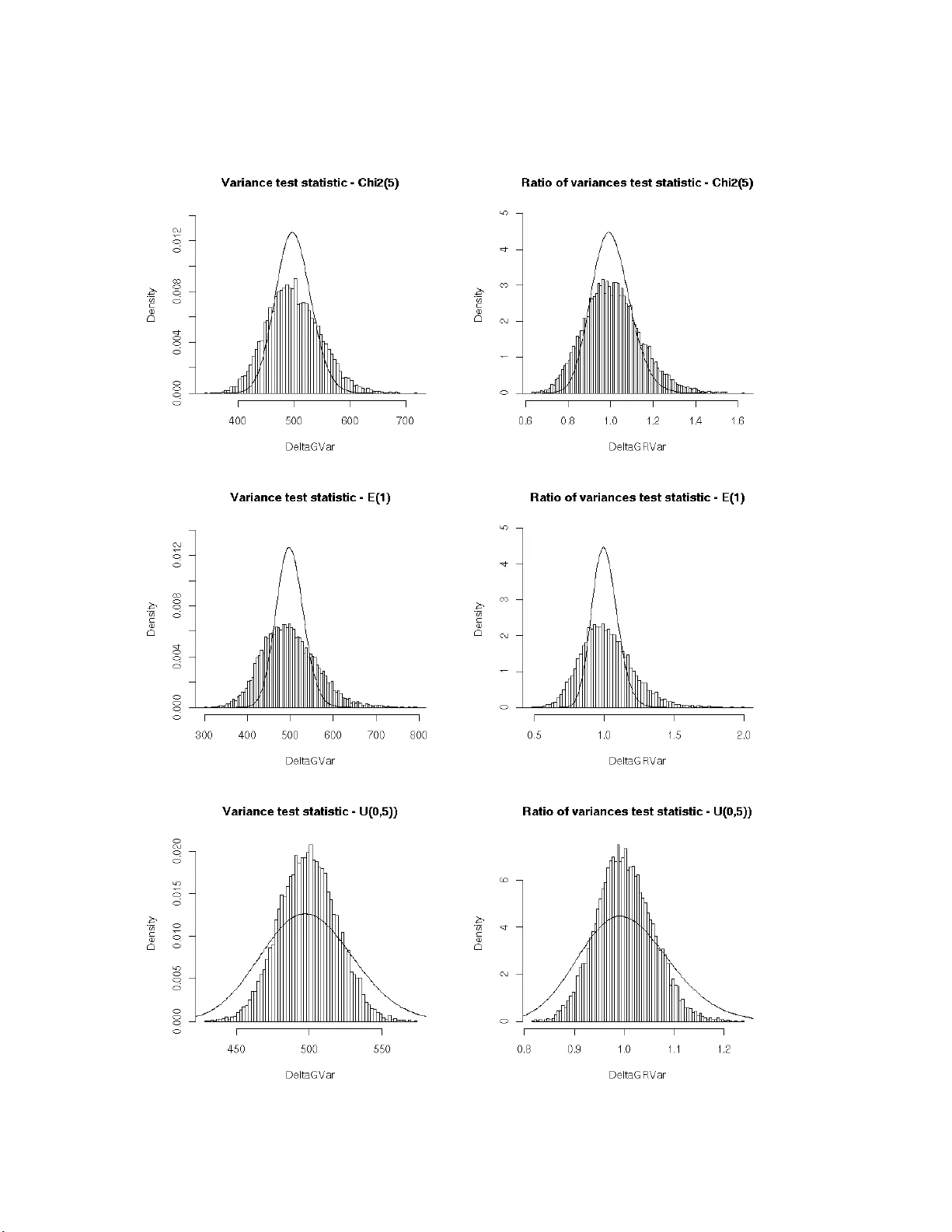
asympTe st : an R p a cka ge f or perfor ming p arametric s t a tistical tests and conf idence inter v als based on the cent ral limit th eorem J.-F. Co eurjolly 1 , R. Drouilhet 1 , P . Lafay e de Mic heaux 1 and J.-F. Robineau 2 1 SAGA G T eam, Lab oratory Jean Kun tzmann/ CNRS, Grenoble ( F rance), 2 CQLS, F ran ce No v em b er 11, 2021 Abstract This pap er describ es an R pack age implemen ting larg e sample tes ts and co nfidence int erv als (based on the central limit theo r em) for v arious pa rameters. The o ne and t wo sample mean and v ariance con texts are considered. The statistics for all the tests are expressed in the same form, which facilitates their pr esentation. In the v ariance pa rameter cases, the asymptotic robustness of the classica l tests dep ends on the departure of the data distr ibutio n from normality mea sured in terms of the kurtosis of the distribution. Keywor ds: p ar ametric tests and c onfidenc e intervals, c entr al limit the or em, R p ackage 1 In tro duction When y ou are in terested in testing a v ariance parameter for a large sample in the non Gaussian framework, it is no t easy to find a test implemen ted in the standard statistical softw a re. In fact, we could not find o ne! The only a v ailable to ol is the chi-square v ar iance test tailo r-made to the Gaussian co n text. This test is how ever commonly used by practicians ev en if the Gaussia n assumption fails. W e applied it to a data set of size n = 1000 with an empirica l distribution very different from a normal distribution. The p-v alue of the c hi-square v a riance test with alternative hypothesis H 1 : σ 2 < 1 is 4.79% which leads us to accept the alternative h yp othesis a t level α = 5%. Is it r easonable to use t his t est when we know that it ca nno t b e used in the no n Gaussian framework because of its sensitivity to departures from normality , e.g. Bo x (1953)? F r om a mathematical p oint of view, one may wonder why no alternative test has b een yet implemen ted since the asymptotic proper ties o f the sample v ariance are w ell-known. Things are m uch e a sier in the sa mple mean study be cause the one s ample t-test is known to b e robust to departures from norma lity for large s amples, e.g. Ozgur and Strasser (200 4). This results fro m a direct application of the central limit theorem. The same rema rks a re v alid when comparing the t wo-sample t-test (diff erence of means test) whic h is robust for la rge s amples and the Fisher test (ratio of v ariances test) which is not. In the statistical framework, one ma y be a s imple use r, a to ol developer , a theoretician or an y combination of the a b ove. There are natural int eractions be tw een thes e different communities and it is expected th at th eir kno wledge should be shared, abov e all for tasks that hav e now bec ome very basic. It is w e ll- known for a theoretician, see e.g. Casella and Ber ger (1990), that a 1 common metho d for constructing a lar ge sample test statistic may be based on an estimato r that has an asymptotic no rmal distribution. Supp ose w e wish to test a hypothesis a bo ut a parameter θ , a nd b θ n is some estimator of θ based o n a sample of size n . If we can prov e s ome form of the central limit theorem to sho w that as n → + ∞ , ( b θ n − θ ) / b σ b θ d → N (0 , 1) where b σ 2 b θ is a con v ergent (in proba bilit y) estimate of V ar ( b θ n ), then o ne has the bas is for an appr oximate test. This scheme based on the central limit theorem will be called the CL T pro cedure. W e hav e alrea dy sp ecified that w e did not find a n y alternative to the chi-square v ariance test for testing a v a riance whe n the normality assumption fails. On the co n trary , the problem of the robustness (to depar tur es from nor malit y) of tests for co mparing tw o (o r more) v a riances has b een widely treated in the literature, see e.g. Bo x (195 3), Conover et a l. (1 981), Tiku et al. (1986), P an (1 999) and the references there in. Some alter native pro cedures to th e F isher test a re implemented in R : the Bartlett test ( bartlet t.test ), the Fligner test ( flign er.test ), the Levene test ( levene.tes t av ailable in the lawstat pack age), etc. How ever to our b est knowledge, for lar ge sa mples, simple alternatives based on the CL T pro cedure hav e never been prop osed or implemen ted. The main ob jectiv e of this pap er is to propos e a unified f ramework, base d on the CL T pro ce- dure, for large samples to test v arious para meter s such as the mean, the v ariance, the difference or r atio of means or v ariances . This appro ach als o allows direct deriv a tion of asymptotic co n- fidence int erv als. T ests and confidence interv als a re then implemented in our new R pack age, called asympTest . This mode s t con tribution also solves the problem of finding a ro bust (to non- normality) alterna tive to the c hi-square v aria nce test for la rge s amples. It also provides a very simple alternative to the Fisher test. How ev er, note that the purp os e of this pap er is no t to compare our tests to their c o mpetitor s in terms o f p ow er. Finally , a firs t course of s tatistical in- ference usually presents mean tests in both Gaussian a nd as ymptotical frameworks and v ariance tests restr icted to the Gaussia n case. The unified appr oach presented here is is very simila r to the classical t-test fro m a ma thematical point of view and giv es us the opp ortunity to prop ose a more complete teaching framew ork with no additiona l difficult y . The pap er is org a nized as follows. Section 2 deals with the mathematical co ncepts and describ es our main no tation. W e also pro po se a mathematica l explanatio n o f the reason why the chi-square v ariance test and the Fisher tes t a r e not appropr iate even when the sample size is very large. Finally , a ge ne r al framework is als o pr op osed that allows us to derive some asymptotic statistical tes ts for the mean, the v ar ia nce and the difference (and ratio) of means o r v ariances. In Section 3, the R pa c k age asym pTest is presented. It no ta bly includes the pro cedures describ ed in the previo us section. Finally , Sectio ns 4, 5 and 6 are devoted to some discussions a nd the pro ofs of our r esults. 2 Mathematical dev elopmen t 2.1 Notation F o r one-sample tests, let us denote by Y = ( Y 1 , . . . , Y n ) a sa mple o f n indep endent and ident ically distributed random v a riables with mean µ and v aria nce σ 2 . These par ameters ar e classically estimated by b µ ( Y ) = Y = 1 n n X i =1 Y i and c σ 2 ( Y ) = 1 n − 1 n X i =1 ( Y i − b µ ( Y ) ) 2 . 2 In the tw o- sample co n text, le t Y ( 1 ) =  Y (1) 1 , . . . , Y (1) n (1)  and Y ( 2 ) =  Y (2) 1 , . . . , Y (2) n (2)  denote tw o independent samples of n (1) and n (2) random v ariable s with r esp ective means µ (1) and µ (2) and v ariance s σ 2 (1) and σ 2 (2) . W e also de fine the following para meter s and their estimated v ersions b y denoting Y =  Y (1) , Y (2)  : • Difference o f (w e ight ed) mea ns: d µ = µ (1) − ρ × µ (2) ( ρ ∈ R ) and c d µ ( Y ) = d µ (1)  Y ( 1 )  − ρ × d µ (2)  Y ( 2 )  . • Difference of (weigh ted) v a riances: d σ 2 = σ 2 (1) − ρ × σ 2 (2) ( ρ ∈ R ) and d d σ 2 ( Y ) = d σ 2 (1)  Y ( 1 )  − ρ × d σ 2 (2)  Y ( 2 )  . • Ratio of means: r µ = µ (1) µ (2) and b r µ ( Y ) = d µ (1) ( Y ( 1 ) ) d µ (2) ( Y ( 2 ) ) . • Ratio of v aria nc e s : r σ 2 = σ 2 (1) σ 2 (2) and c r σ 2 ( Y ) = d σ 2 (1) ( Y ( 1 ) ) d σ 2 (2) ( Y ( 2 ) ) . The known pa r ameter ρ is, in our definitio n of d µ and d σ 2 , in trinsically nonnega tive. But note that there is no mathematical problem to dea l with negative v alues of ρ . In order to compare the Gaussia n fra mew ork and the genera l o ne, w e pr op ose to deno te b y Y G (resp. Y (1) ,G , Y (2) ,G ) a vector (resp. t w o indep endent vectors) of n (r esp. n (1) and n (2) ) Gaussian rando m v ariables with mean µ (resp. µ (1) and µ (2) ) and v ariance σ 2 (resp. σ 2 (1) and σ 2 (2) ). In the t wo-sample context, let us also denote Y G =  Y (1) ,G , Y (2) ,G  . In the sequel, w e will use the nota tion := to define so me quan tit y . F or some ra ndom v ariable Z and some distribution L , Z L (resp. appro x L ) means that Z follows (resp. approximately follows) the distribution L . 2.2 Ab out the Chi-square and Fisher tests In this section, we conc e ntrate on par ameters σ 2 and r σ 2 . The cla s sical s tatistics of the chi-square test of v ar iance and the Fisher test of ratio of v aria nces are defined by Λ G c σ 2 ,σ 2 ( Y ) := ( n − 1) c σ 2 ( Y ) σ 2 and Λ G d r σ 2 ,r σ 2 ( Y ) := c r σ 2  Y ( 1 ) , Y ( 2 )  r σ 2 . The notation Λ G c σ 2 ,σ 2 expresses that the statistic is a measure of the departure of c σ 2 from σ 2 in the Gaussia n framework. When the data a re Gaussian, it is well-known that Λ G c σ 2 ,σ 2 ( Y G ) χ 2 ( n − 1) and Λ G d r σ 2 ,r σ 2 ( Y G ) F  n (1) − 1 , n (2) − 1  . How ever, as shown in Fig. 1 , b oth r esults b ecome unt rue (ev en a pproximately) under non- normality assumption. The theoretical reason may b e explained as follows. Let n (1) = n and assume tha t there exists α > 0 s uch that n (2) = αn (1) . Assume also that Y (resp. Y (1) and Y (2) ) has a finite kur tosis k := E (( Y − µ ) 4 ) /V ar ( Y ) (resp. k (1) and k (2) ). Then, as n → + ∞ , Λ G c σ 2 ,σ 2 ( Y ) − ( n − 1) √ n − 1 d − → N ( 0 , k − 1) (1) √ n  Λ G d r σ 2 ,r σ 2 ( Y ) − 1  d − → N  0 , k (1) − 1 + k (2) − 1 α  . (2) 3 This result is a consequence of a more general o ne sta ted in Section 2.3 and pr ov ed in Section 6. Equations (1) a nd (2) lea d to the following approximations Λ G c σ 2 ,σ 2 ( Y ) appro x N ( n − 1 , ( k − 1)( n − 1)) and Λ G d r σ 2 ,r σ 2 ( Y ) appro x N  1 , k (1) − 1 n (1) + k (2) − 1 n (2)  . When data ar e Gaussian ans when n is la rge, one obtains the w e ll-known a ppr oximations χ 2 ( n − 1) ≃ N ( n − 1 , 2( n − 1)) and F  n (1) , n (2)  ≃ N  1 , 2 n (1) + 2 n (2)  since k = k (1) = k (2) = 3 W e ca n underline that Λ G c σ 2 ,σ 2 ( Y ) (resp. Λ G d r σ 2 ,r σ 2 ( Y )) and Λ G c σ 2 ,σ 2 ( Y G ) (resp. Λ G d r σ 2 ,r σ 2 ( Y G )) differ in terms o f asymptotical v ariances. More precisely , the gap betw ee n the tw o framew orks is essentially g ov er ned by the kurtosis . Indeed, as n → + ∞ V ar (Λ G c σ 2 ,σ 2 ( Y )) V ar (Λ G c σ 2 ,σ 2 ( Y G )) → k − 1 2 and V ar (Λ G d r σ 2 ,r σ 2 ( Y )) V ar (Λ G d r σ 2 ,r σ 2 ( Y G )) → k (1) − 1 + k (2) − 1 α 2  1 + 1 α  . T ab. 1 proposes the c o mputations of these a symptotic ratios for different distributions. This allows the rea de r to asses s the r isk of using the cla s sical statistics Λ G c σ 2 ,σ 2 and Λ G d r σ 2 ,r σ 2 under the non-normality a ssumption even when the size of the sa mple is large. Y d = Y (1) d = Y (2) L T est L = χ 2 ( ν ) L = E ( λ ) L = U ([ a, b ]) V a riance test 1 + 6 ν 4 2 5 Ratio of v aria nces test 1 + 6 ν 4 2 5 T able 1: Ratio of a symptotic v ariances (non gaussia n/gaussia n) k − 1 2 and k (1) − 1+ k (2) − 1 α 2 ( 1+ 1 α ) in the case where k = k (1) = k (2) and α = 1. 2.3 Large sa mple tests based on t he central limit theorem The pa rameters σ 2 , d µ and d σ 2 can b e viewed as particula r means. Therefor e, the idea (widely used in a symptotic theor y ) is to design a symptotic tests and confidence in terv als thanks to the central limit theo rem. The v ariables b r µ ( Y ) − r µ and c r σ 2 ( Y ) − r σ 2 can also b e expressed in terms of means to which a central limit theorem can be applied. In or der to unify a symptotic results, we define θ as one of the parameters µ , σ 2 , d µ , d σ 2 , r µ and r σ 2 . B y applying a cen tral limit theorem, the law of large num b ers a nd Slutsky’s theo rem (see Section 6), o ne obtains, as n → + ∞ , b ∆ b θ ,θ ( Y ) := b θ ( Y ) − θ c σ b θ ( Y ) d − → N (0 , 1) , (3) where c σ b θ ( Y ) is the standar d er ror of b θ ( Y ). The assumptions under whic h the c e n tral limit theorem can b e applied and the de finitio n of c σ b θ ( Y ) are stated in T ab. 2. R functions have b een implemen ted to ev alua te the standard erro rs of the estimates of θ , s ee T ab. 3. 4 Figure 1: Histograms of m = 10000 replications of test sta tistics o f v ariance test ( left) and ratio of v ariance tests (righ t) in the Gaus sian con text. The simulation ha s b een done as follows: n = n (1) = n (2) = 500, Y d = Y (1) d = Y (2) χ 2 (5) (top), E (1) (middle) and U ([0 , 5]) (bottom). 5 θ Assumptions c σ b θ ( Y ) µ E  Y 2 i  < + ∞ s c σ 2 ( Y ) n σ 2 E  Y 4 i  < + ∞ v u u t c σ 2 ¨ Y  ¨ Y  n d µ E   Y ( j ) i  2  < + ∞ , j = 1 , 2 s d σ 2 (1)  Y ( 1 )  n (1) + ρ 2 × d σ 2 (2)  Y ( 2 )  n (2) d σ 2 E   Y ( j ) i  4  < + ∞ , j = 1 , 2 v u u t [ σ 2 ¨ Y (1)  ¨ Y ( 1 )  n (1) + ρ 2 × [ σ 2 ¨ Y (2)  ¨ Y ( 2 )  n (2) r µ µ (2) 6 = 0, E   Y ( j ) i  2  < + ∞ , j = 1 , 2 1 ˛ ˛ ˛ d µ (2) ( Y ( 2 ) ) ˛ ˛ ˛ r d σ 2 (1) ( Y ( 1 ) ) n (1) + b r µ ( Y ) 2 × d σ 2 (2) ( Y ( 2 ) ) n (2) r σ 2 σ 2 (2) 6 = 0, E   Y ( j ) i  4  < + ∞ , j = 1 , 2 1 d σ 2 (2) ( Y ( 2 ) ) r \ σ 2 ¨ Y (1) ( ¨ Y ( 1 ) ) n (1) + c r σ 2 ( Y ) 2 \ σ 2 ¨ Y (2) ( ¨ Y ( 2 ) ) n (2) T able 2 : Standar d er rors of estimates of θ . F or the sa ke of s implicit y we denote by ¨ Y := ( Y − µ ) 2 , ¨ Y := ( Y − b µ ( Y )) 2 , σ 2 ¨ Y := V ar  ¨ Y  and c σ 2 ¨ Y  ¨ Y  := 1 n − 1 P n i =1  ( Y i − b µ ( Y ) ) 2 − c σ 2 ( Y )  2 . θ Dataset(s) c σ b θ ( y ) in R µ y seMean (y) σ 2 y seVar( y) d µ y1 , y2 seDMea n(y1,y 2,rho=1) d σ 2 y1 , y2 seDVar (y1,y2 ,rho=1) r µ y1 , y2 seRMea n(y1,y 2) r σ 2 y1 , y2 seRVar (y1,y2 ) T able 3: Standard err ors of estimates of θ in R . 6 Remark 1 The figur es Fig. 2, Fig. 3 and Fig. 4 al low the r e ader to il lustr ate the mathematic al r esult (3). Remark 2 The asymp totic r esult (3) a l lows us to e asily c onst ruct statistic al hyp othesis tests and c onfidenc e intervals, se e e.g. Ca sel la and Ber ger (199 0) p. 385 for development. Remark 3 The alternative hyp othesis H 1 c omp aring the r atio of me ans or varianc es t o some r efer enc e value r 0 may b e expr esse d in t erms of t he c omp arison of the weigh te d differ enc es d µ := µ (1) − r 0 µ (2) or d σ 2 := σ 2 (1) − r 0 σ 2 (2) to 0, t he value of ρ b eing fixe d to r 0 . 3 Using asympT est The R pack age asy mpTest consists of a main function asym p.test a nd s ix auxiliary ones designed to compute standard erro rs of estima tes of different para meters, see T ab. 3. The auxiliary func- tions should not b e very useful for the use r, except if he/s he w ant s to compute himse lf/ herself the confidence interv al. The function a symp.t est has b een written in t he same spirit as the R functions t.te st or va r.test . The arguments of a symp.t est , its v alue and the result- ing outputs are inspired fr o m the ones o f t.tes t o r var.t est . In particular , the function asympt .test r eturns an ob ject of class “ h test” (which is the general class o f test ob jects in R , see R Developmen t Core T eam (2004)). The main arguments of the function asymp .test a re: • x : vector of data v alues. • y : optional vector of data v alues . • paramet er : parameter under testing , must b e o ne of “mean” , “v ar ” , “dMean” , “dV ar” , “rMean” , “r V a r” . • alterna tive : alterna tive hypothesis, must be one of “tw o .sided” (default), “gr eater” or “less” . • referen ce : reference v alue of the parameter under the null h ypo thesis. • conf.le vel : confidence level o f the interv al (default is 0.95 ). The type-one er ror is then fixed to 1- con f.leve l . • rho : optio nal parameter (only used for parameters ” dMean” a nd ” dV a r” ) for p enalization (or enhancement) of the contribution of the second parameter. The user may only sp e cify the first letters of the parameter or alterna tiv e. In order to illustrate this function, let us consider the i ris data av ailable in R . This famous (Fisher’s or Anderson’s Fisher (1935); Ander son (1935)) da ta set g ives the measuremen ts (in centim eters) o f the four v a riables sepa l length and width, and p etal leng th a nd width, for 50 flow er s from each s pecie s of iris: se tosa, versicolor, and virginica. 1 > data(i ris) 2 > attach (iris) 3 > names( iris) 4 [1] "Sepal .Lengt h" "Sepal.Wid th" "Petal.Len gth" "Petal. Width" "Specie s" 5 > levels (iris$ Species) 6 [1] "setos a" "versi color" "virg inica" 7 Figure 2 : Histog rams of m = 1 0000 replications of b θ ( Y ) − θ c σ b θ ( Y ) for θ = µ , σ 2 , d µ , d σ 2 , r µ and r σ 2 . The simulation has been done as follows: n = n (1) = n (2) = 50 0, Y (1) χ 2 (5), Y (2) χ 2 (5). 8 Figure 3 : Histog rams of m = 1 0000 replications of b θ ( Y ) − θ c σ b θ ( Y ) for θ = µ , σ 2 , d µ , d σ 2 , r µ and r σ 2 . The simulation has been done as follows: n = n (1) = n (2) = 50 0, Y (1) E (1 ), Y (2) E (1 ). 9 Figure 4 : Histog r ams o f m = 100 00 replica tions of b θ ( Y ) − θ c σ b θ ( Y ) for θ = µ , σ 2 , d µ , d σ 2 , r µ and r σ 2 . The simulation has been done as follo ws: n = n (1) = n (2) = 500, Y (1) U ([0 , 5]), Y (2) E (0 . 5). 10 Sepal.Length Sepal.Width Petal.Length Petal.Width setosa 0.4595 0.2715 0.0548 0.0000 versicolor 0.4647 0.3380 0.1585 0.0273 virginica 0.258 3 0.1809 0.1098 0.0870 The following table presents the p-v alues of a ll the Shapiro-Wilk nor mality tests for the different v ariables and the three species . Let us concentrate on the v ariable Petal.Width for w hich the Gaussia n assumption seems to be wrong for each one of the three sp ecies. The empirical means and v aria nces are given b elow: 1 > by(Pet al.Wid th,Species,function(e) c(m ean=mea n(e),var=var(e))) 2 Specie s: se tosa 3 mean var 4 0.2460 0000 0. 011106 12 5 ------ ------ ------------------------ ------------------------ 6 Specie s: ve rsicol or 7 mean var 8 1.3260 0000 0. 039106 12 9 ------ ------ ------------------------ ------------------------ 10 Specie s: vi rginic a 11 mean var 12 2.0260 0000 0. 075432 65 Is the mean p etal width o f setosa sp ecies less than 0 . 5 ? 1 > requir e(asym pTest) 2 > asymp. test(P etal.Width[Species=="s etosa"],par="mean",alt="l",ref= 0.5) 3 4 One-sa mple as ymptot ic mean test 5 6 data: Petal.Wi dth[Species == "setosa"] 7 statis tic = -17 .0427, p -value < 2.2e-16 8 altern ative hyp othesis : true mean is less t han 0.5 9 95 perce nt co nfiden ce interva l: 10 -Inf 0.2705 145 11 sample estima tes: 12 mean 13 0.246 Is the mean p etal width o f virginica sp ecies lar ger than the versicolor one ? 1 > asymp. test(P etal.Width[Species=="v irginica"], 2 + Petal. Width[ Species=="versicolor"] ,"dMean","g",0) 3 4 Two-sa mple as ymptot ic differe nce of means test 5 6 data: Petal.Wi dth[Species == "virginic a"] and Petal.W idth[S pecies == "ver sicolo r"] 7 statis tic = 14. 6254, p-value < 2. 2e-16 8 altern ative hyp othesis : true differe nce of means is greater than 0 11 9 95 perce nt co nfiden ce interva l: 10 0.6212 74 Inf 11 sample estima tes: 12 differ ence of mean s 13 0.7 Is the mean p etal width o f virginica sp ecies 4 times la rger than the setos a one ? 1 > asymp. test(P etal.Width[Species=="v irginica"], 2 + Petal. Width[ Species=="setosa"],"rM ean","g",4) 3 4 Two-sa mple as ymptot ic ratio of means test 5 6 data: Petal.Wi dth[Species == "virginic a"] and Petal.W idth[S pecies == "set osa"] 7 statis tic = 8.0 936, p -value = 3.331e-16 8 altern ative hyp othesis : true ratio of means i s greate r than 4 9 95 perce nt co nfiden ce interva l: 10 7.3749 46 Inf 11 sample estima tes: 12 ratio of means 13 8.2357 72 This may also be do ne via a difference of w eight ed means test. 1 > asymp. test(P etal.Width[Species=="v irginica"], 2 + Petal. Width[ Species=="setosa"],"dM ean","g",0,rho=4) 3 4 Two-sa mple as ymptot ic differe nce of (weig hted) me ans test 5 6 data: Petal.Wi dth[Species == "virginic a"] and Petal.W idth[S pecies == "set osa"] 7 statis tic = 14. 6447, p-value < 2. 2e-16 8 altern ative hyp othesis : true differe nce of (weigh ted) means is great er th an 0 9 95 perce nt co nfiden ce interva l: 10 0.9249 653 Inf 11 sample estima tes: 12 differ ence of (wei ghted) means 13 1.042 4 T yp e I error risks 4.1 Comparison betw een clas sical an d asymptotic v ariance tests In the context of larg e samples, t w o simulation studies are prop osed in order to show the lack of reliability of the classica l tests for v ariance parameter s compar e d with the as y mptotic tests studied in this pa per . F or each of the following examples, 1000 0 simulations of s amples of size n = 1000 hav e been p erfor med. 1. Let us consider testing H 0 : σ 2 = 1 versus H 1 : σ 2 < 1 with da ta sampled fro m distribution E (1) (i.e., under H 0 ). In the ca se w he r e α = 5%, the probability of accepting the alter native hypothesis is 8.91% for the asymptotic test and 20.99% for the chi-square test. 12 false true false 0.7901 0.000 0 true 0 .1208 0.089 1 T able 4: Acceptance of H 1 for the chi-square test (rows) v er sus the asymptotic test (columns) 2. Let us consider test H 0 : σ 2 (1) = σ 2 (2) versus H 1 : σ 2 (1) 6 = σ 2 (2) with da ta sampled from distribution U ([0 , 5 ]) for both samples (i.e., under H 0 ). false true false 0.9498 0.048 1 true 0 .0000 0.002 1 T able 5: Acceptance of H 1 for the Fisher test (r ows) versus the asymptotic test (columns) In the ca se w he r e α = 5%, the probability of accepting the alter native hypothesis is 5.02% for the asymptotic test and 0.21% for the Fisher test. In b oth case s , the probabilities for Type I err ors a re worse for the classic al tests than for the corres p onding w ell-suited asymptotic tests. This is a direct consequence of the previo us results summarized by figure Fig. 1. 4.2 Bac k to the example of the in tro duction Now, one may wonder w ha t the cons equences of these previous results are for pratical purpos es. Let us consider ag ain the ex ample presented in the in troductio n. In order to illustrate the tw o- samples case, we pro po se a second e xample. In the fo llowing R outputs, the data of the first (resp. seco nd) example are denoted by y (resp. y1 and y2 ). These s amples have a size n=1000 and their empiric a l distributions, prop osed below, do not s eem to fit normal distr ibutions. The following o utput provides the p-v alue of the chi-square test for the fir st example. 1 > pchisq ((leng th(y)-1)*var(y)/1,leng th(y)-1) 2 [1] 0.0478 5152 Due to the appar en t no n nor mality of the data, one may prefer to a pply the corre s po nding asymptotic test: 13 1 > asymp. test(y ,par="var",alt="l",ref =1) 2 3 One-sa mple as ymptot ic varianc e tes t 4 5 data: y 6 statis tic = -0. 9771, p-value = 0. 1643 7 altern ative hyp othesis : true varianc e is less than 1 8 95 perce nt co nfiden ce interva l: 9 -Inf 1. 070430 10 sample estima tes: 11 varian ce 12 0.8969 455 The t wo decisions do no t ma tch, but since the empir ic al v a r iance is 0.896945 5, o ne may think that σ 2 is sligh tly infer ior to 1 . In which ca se, w e hav e to b e cautious b eca us e our sa mple migh t be of the same kind as the 12.08% of T able 4. The following o utput provides the p-v alue of the Fisher test for the second example. 1 > var.te st(y1, y2) 2 3 F test to compare two variances 4 5 data: y1 and y2 6 F = 0.8874 , num df = 499, denom df = 499, p-value = 0 .1825 7 altern ative hyp othesis : true ratio of variances is n ot equal to 1 8 95 perce nt co nfiden ce interva l: 9 0.744 4324 1.0 578390 10 sample estima tes: 11 ratio of varianc es 12 0.8874 061 Due to the appar en t no n nor mality of the data, one may prefer to a pply the corre s po nding asymptotic test: 1 > asymp. test(y 1,y2,"dVar") 2 3 Two-sa mple as ymptot ic differe nce of varia nces tes t 4 5 data: y1 and y2 6 statis tic = -2. 0925, p-value = 0. 03639 7 altern ative hyp othesis : true differe nce of varian ces is not equal to 0 8 95 perce nt co nfiden ce interva l: 9 -0.499 88046 -0. 0163530 5 10 sample estima tes: 11 differ ence of vari ances 12 -0.258 1168 The t wo decisions do not matc h, but since the empirical v aria nces ar e 2.0 34341 and 2.292 458, one may think that σ 2 (1) and σ 2 (2) are slightly different . In which case, we have to b e cautious bec ause our sa mple might be of the same kind as the 4.81% of T able 5. 14 5 Discussion W e have pr esented an R pa ck age implemen ting lar ge sample tests for v arious par ameters. The int eresting po int is that each test statistic can be written in the same for m, as follows: b ∆ b θ,θ ( Y ) := b θ ( Y ) − θ c σ b θ ( Y ) . This form clear ly expresses the departur e of the estimate fro m the true para meter, nor malized by some q ua n tit y measuring the pr e cision of the estima te. This appro ach is th en attra ctive and easy to pres e nt. In the Gaussia n framework, the one and t wo-sample t-tests follow this idea whereas the chi-square v ariance test and the Fisher test do not. O ne may wonder if it is p oss ible to embed the classical Gaus s ian framework within this formalism. Mo re precisely , for an estimate b θ ( Y ) of some para meter θ with standar d deviation σ b θ = q V ar ( b θ ( Y )), let us propo se the test statistic ∆ b θ ,θ ( Y ) := b θ ( Y ) − θ σ b θ or b θ ( Y ) − θ e σ b θ (4) in the case where σ b θ or po ssibly some known a symptotic equiv alent e σ b θ of σ b θ only depends o n θ , or b ∆ b θ ,θ ( Y ) := b θ ( Y ) − θ c σ b θ ( Y ) (5) otherwise, where c σ b θ ( Y ) is a consistent estimate of σ b θ . In the larg e s ample f ramework, the parameters µ , σ 2 , d µ , r µ , d σ 2 and r σ 2 fall in to the case of equation (5) a nd the co rresp onding statistic approximately follows a N (0 , 1) distribution. In this same context, the prop or tion par ameter falls into the ca s e of eq uation (4) with σ b p = p p (1 − p ) / n . In the Ga ussian framework, the parameter s µ and d µ leading to the one-s a mple and tw o- sample t-tests also fall in to the case of equa tion (5). Let us now co ncent rate o n parameters σ 2 and r σ 2 (corresp onding to the c hi-square v ar iance test and the Fisher test). It is known that the v ariance of c σ 2  Y G  and an as ymptotic equiv alent o f the v a r iance of c r σ 2  Y G  are of the fo r m σ 2 c σ 2 = 1 n  ˙ µ 4 − n − 3 n − 1 ˙ µ 2 2  and e σ 2 d r σ 2 = 1 n (1) ˙ µ (1) 4 − ( ˙ µ (1) 2 ) 2 ( ˙ µ (2) 2 ) 2 + 1 n (2) r 2 σ 2 ˙ µ (2) 4 − ( ˙ µ (2) 2 ) 2 ( ˙ µ (2) 2 ) 2 where ˙ µ k = E  ( Y − E ( Y )) k  is the k − th ce n tered momen t of Y (with our notation ˙ µ 2 = σ 2 ). F o r Gaussian v ar iables, ˙ µ 4 = 3( ˙ µ 2 ) 2 which leads to σ 2 c σ 2 = 2 n − 1 σ 4 and e σ 2 d r σ 2 = 2 r 2 σ 2  1 n (1) + 1 n (2)  . Now, in order to build a test, let us giv e the distributions o f ∆ G c σ 2 ,σ 2 ( Y G ) and ∆ G d r σ 2 ,r σ 2 ( Y G ) expressed in terms o f Λ G c σ 2 ,σ 2 ( Y G ) and Λ G d r σ 2 ,r σ 2 ( Y G ): ∆ G c σ 2 ,σ 2 ( Y G ) := c σ 2  Y G  − σ 2 σ c σ 2 = Λ G d σ 2 ,σ 2 ( Y G ) n − 1 σ 2 − σ 2 σ 2 p 2 / ( n − 1) χ 2 ( n − 1) − ( n − 1) p 2( n − 1 ) and ∆ G d r σ 2 ,r σ 2 ( Y G ) := c r σ 2  Y G  − r σ 2 e σ d r σ 2 = r σ 2 Λ G d r σ 2 ,r σ 2 ( Y G ) − r σ 2 r σ 2 p 2 /n (1) + 2 /n (2) F ( n (1) − 1 , n (2) − 1 ) − 1 p 2 /n (1) + 2 /n (2) . 15 One may pr op ose a name for the prev io us tw o free distributio ns : centered reduced chi-square distribution a nd centered reduced Fisher distribution resp ectively deno ted by χ 2 cr ( · ) and F cr ( · , · ). If these distr ibutions were implemen ted such that one may ev aluate quan tiles and p-v a lues, one could build t wo new tests directly bas ed on ∆ G c σ 2 ,σ 2 ( Y G ) a nd ∆ G d r σ 2 ,r σ 2 ( Y G ). O f course , these tw o new tests would b e stric tly equiv alent to the class ical c hi-square v aria nce test and Fis her tes t and would then fall into the same formalism. Let us now commen t on the concept o f ro bus tness in the Ga ussian fra mework. In the par - ticular ca se of mean hypothesis testing, this ro bustness is expressed by the fact that ∆ G b µ,µ ( Y G ) is equal to ∆ b µ,µ ( Y G ) with the same a symptotic distribution N (0 , 1). When considering the t w o new ca ses θ = σ 2 or θ = r σ 2 , ∆ G b θ ,θ ( Y G ) is no lo ng er equal to ∆ b θ,θ ( Y G ) but hav e at le ast the same asymptotic distribution N (0 , 1). How ever, one can pr ov e that ∆ G b θ ,θ ( Y G ) and ∆ b θ ,θ ( Y G ) are asymptotically equiv alent in probability , which may b e v ie w ed as some kind of robustness. 6 Pro ofs In this sec tio n, w e o nly pr ov e (3). The results (1) a nd (2) ar e direct cons equences. Recall that for ea c h para meter, some a ssumptions a r e needed essen tially in order to apply the cen tral limit theorem. They are summarized in T ab. 2. P arameter µ : This is a direct application of the central limit theorem. P arameter σ 2 : By definition c σ 2 ( Y ) − σ 2 = 1 n − 1 n X i =1   Y i − Y  2 − σ 2  = 1 n − 1 n X i =1  ( Y i − µ ) 2 − σ 2  − n n − 1  Y − µ  2 . F r om the CL T, the law of large num b ers and Slutsky’s Theorem (see e.g. F erguson (199 6)) , it comes that as n → + ∞ √ n  Y − µ  2 P − → 0 . Therefore, as n → + ∞ , √ n  c σ 2 ( Y ) − σ 2  d − → N (0 , V ar (( Y − µ ) 2 )) . Since σ c σ 2 := q V ar (( Y − µ ) 2 ) n can b e co nsistently estimated by d σ c σ 2 ( Y ) := r c σ 2 ¨ Y ( ¨ Y ) n , s ee T ab. 2, we obtain as n → + ∞ b ∆ c σ 2 ,σ 2 ( Y ) := c σ 2 ( Y ) − σ 2 d σ c σ 2 ( Y ) d − → N (0 , 1) . P arameter d µ : Recall that n = n (1) and n (2) = αn (1) . As n → + ∞ , √ n  c d µ ( Y ) − d µ  = √ n  d µ (1)  Y ( 1 )  − µ (1)  − ρ × √ nα √ α  d µ (2)  Y ( 2 )  − µ (2)  d − → N 0 , σ 2 (1) + ρ 2 × σ 2 (2) α ! . 16 Since σ c d µ := r σ 2 (1) + ρ 2 × σ 2 (2) α n can b e consis tently estimated by d σ c d µ ( Y ) := s d σ 2 (1)  Y ( 1 )  n (1) + ρ 2 × d σ 2 (2)  Y ( 2 )  n (2) , we o btain as n → + ∞ b ∆ c d µ ,d µ ( Y ) := c d µ ( Y ) − d µ d σ c d µ ( Y ) d − → N (0 , 1) . P arameter d σ 2 : As n → + ∞ , √ n  d d σ 2 ( Y ) − d σ 2  = √ n  \ σ 2 (1) (1)  Y ( 1 )  − σ 2 (1)  − ρ × √ nα √ α  d σ 2 (2)  Y ( 2 )  − σ 2 (2)  d − → N 0 , σ 2 ¨ Y (1) + ρ 2 × σ 2 ¨ Y (2) α ! . Since σ d d σ 2 := s σ 2 ¨ Y (1) + ρ 2 σ 2 ¨ Y (2) α n can b e consis tently estimated by d σ d d σ 2 ( Y ) := v u u t [ σ 2 ¨ Y (1)  ¨ Y ( 1 )  n + ρ 2 × [ σ 2 ¨ Y (2)  ¨ Y ( 2 )  nα = v u u t [ σ 2 ¨ Y (1)  ¨ Y ( 1 )  n (1) + [ σ 2 ¨ Y (2)  ¨ Y ( 2 )  n (2) , we o btain as n → + ∞ d d σ 2 ( Y ) − d σ 2 d σ d d σ 2 ( Y ) d − → N (0 , 1) . P arameter r µ : Using Slutsky’s Theor e m, one ma y assert that as n → + ∞ √ n ( b r µ ( Y ) − r µ ) = √ n d µ (1)  Y ( 1 )  d µ (2)  Y ( 2 )  − µ (1) µ (2) ! = √ n d µ (1)  Y ( 1 )  − µ (1) d µ (2)  Y ( 2 )  + µ (1) 1 d µ (2)  Y ( 2 )  − 1 µ (2) !! n → + ∞ ∼ √ n d µ (1)  Y ( 1 )  − µ (1) µ (2) + √ nα √ α µ (1) ( µ (2) ) 2  µ (2) − d µ (2)  Y ( 2 )  ! d − → N 0 , σ 2 (1) ( µ (2) ) 2 +  µ (1) ( µ (2) ) 2  2 σ 2 (2) α ! . 17 Since, σ c r µ := s σ 2 (1) ( µ (2) ) 2 + „ µ (1) ( µ (2) ) 2 « 2 σ 2 (2) α n can b e consis tently estimated by d σ c r µ ( Y ) := v u u u t d σ 2 (1) ( Y ( 1 ) ) d µ (2) ( Y ( 2 ) ) n +  d µ (1) ( Y ( 1 ) ) d µ (2) ( Y ( 2 ) ) 2  2 d σ 2 (2)  Y ( 2 )  nα = 1 d µ (2)  Y ( 2 )  s d σ 2 (1)  Y ( 1 )  n (1) + b r µ ( Y ) d σ 2 (2)  Y ( 2 )  n (2) we o btain as n → + ∞ , b r µ ( Y ) − r µ d σ c r µ ( Y ) d − → N (0 , 1) . P arameter r σ 2 : The pr o of follows the ideas dev elop e d for the pa r ameters σ 2 , d σ 2 and r µ , a nd thus is left to the reader . Ac kn o wledgmen ts W e would like to thank Laurence P ierret fo r having kindly reread our English. She could in no wa y b e held respo nsible for any remaining mistak es. References E. Anderso n. The ir ises of the gasp e p eninsula. Bul letin of the Americ an Iris S o ciety , 59:2–5 , 1935. G.E.P . Bo x. Non-normality and tests on v ar ia nces. Biometrika , 40(3/ 4):318– 335, 1953. G. Casella and R.L. Berger. Statist ic al Infer en c e . Duxbury press, Belmon t, California, 1990 . W.J. C o nov er , M.E . J ohnson, a nd M.M. Johnson. A comparative study of tests for homogeneity of v ariances with applica tions to the outer continen ta l shelf bidding data. T e chnometrics , 23 (4):351–3 61, 1 981. T.S. F erguson. A c ourse in lar ge s ample the ory . Chapma n and Hall, London, UK , 1 996. R.A. Fisher. The use o f m ultiple meas urements in taxonomic problems. Annals of Eugenics , 7 (Part I I):17 9–188 , 1 935. C. O zgur a nd S.E . Stra sser. A study of the statistical inference criteria: can w e a gree o n when to use z versus t ? D e cision Scienc es Journal of Innovative Educ ation , 2(2):177–19 2, 2004 . G. Pan. On a levene t ype test for equalit y of tw o v aria nces. Journal of St atistic al Computation and Simulation , 63:59– 71, 1 999. R Dev elo pmen t Core T eam. R: A L anguage and Envir onment for S t atistic al Computing . R F o undation for Statistical Co mputing, Vienna, Austria, 2004. ISBN ISBN 3-9 00051 -00-3 . URL http ://www .R- project.org/ . 18 M.L. Tiku, W .Y. T an, and N. Balakrishnan. R obust infer enc e . Statis tics : T extb o oks and Mo no- graphs, New Y ork, USA, 198 6. 19