Generalization of Jeffreys divergence based priors for Bayesian hypothesis testing

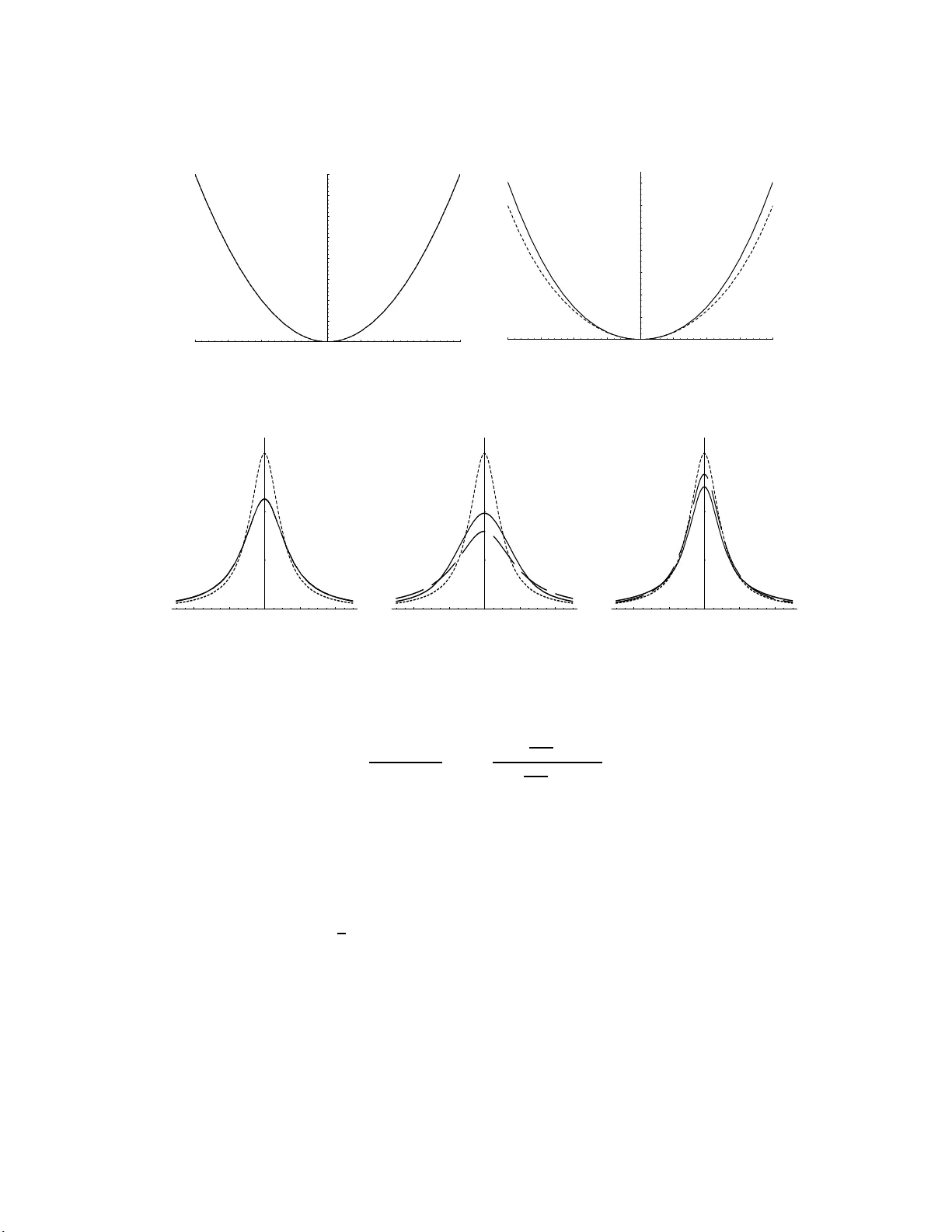
Generalizati o n of Jeﬀreys’ Div ergence B ased Priors for Ba y esian Hyp othesi s tes ting M.J. Ba y arri Univ ersit y o f V alencia G. Garc ´ ıa-Donato Univ ersit y of Castilla-La Manc ha ∗ August 3, 2018 Abstract In this pap er we int ro duce ob jective prop er prio r dis tributions for hypothes is testing and mo del selection based on meas ures of divergence b et ween the comp eting mo dels; we call them diver genc e b ase d (DB) prior s. DB priors ha ve simple forms and desirable prop erties, like information (ﬁnite sample) consistency; o ften, they a re similar to other existing prop osals like the intrinsic prio rs; mo reov er, in nor mal linear mo dels scenar ios, they e x actly r epro duce Jeﬀreys-Ze llne r -Siow prio rs. Most imp ortantly , in challenging scenarios such as irreg ular mo dels and mixture mo dels , the DB pr iors are w ell deﬁned and very reasona ble, while alternative prop osa ls are not. W e der ive approximations to the DB prio rs as well as MCMC and asymptotic expressio ns for the asso ciated Bayes factors . Keyw ords : Bay es factors ; Infor ma tion Consistency; In trinsic prior s; Ir regular mo dels; Kullback-Leibler divergence; Mix ture models. 1 In tro duction F or the data y , with den s it y f ( y | θ , ν ), w e consider the h yp othesis testing problem: H 1 : θ = θ 0 , vs. H 2 : θ 6 = θ 0 , (1) where θ 0 ∈ Θ is a known v alue. This is equiv alen t to the mo del selection p roblem of c ho osing b et wee n mo dels: M 1 : f 1 ( y | ν 1 ) = f ( y | θ 0 , ν 1 ) vs. M 2 : f 2 ( y | θ , ν 2 ) = f ( y | θ , ν 2 ) , (2) ∗ Address for correspondence: Gonzalo Garc ´ ıa-Donato, Department of Economy , Plaza Universidad 2, 02071 Albacete, S pain. Email:Gonzalo.Ga rciaDonato@uclm.es 1 where the notation r eﬂects the fact th at often ν 1 and ν 2 represent diﬀerent quan tities in eac h mo del. In Jeﬀreys’ scenarios (Jeﬀreys, 19 61), ν 1 and ν 2 had the same mea nin g; he ca lled θ the new p ar ameter , and ν 1 and ν 2 , the c ommon p ar ameters (also known as nuisance parameters). W e r evisit this issue in Section 4. W e aim for an obje ctive Bayes solution to this m o del selection problem; that is, no ‘external’ (sub jectiv e) inform ation is assumed, other than the data, y , and th e in formation implicitly needed to p ose the pr oblem, c ho ose the comp eting mo dels, etc. An excellen t exp osition of the adv ant ages of Ba y esian metho ds, sp ecially ob jectiv e Ba y es metho ds, f or pr oblems with mo d el uncertain t y is Berger and Pericc hi (2001). Usual Ba ye sian s olutions (for 0- k i loss fun ctions) to (1) (or, equiv alen tly , to (2)) are based on the p osterior odd s: Pr( H 1 | y ) Pr( H 2 | y ) = Pr( H 1 ) Pr( H 2 ) × B 12 , where Pr( H i ) , i = 1 , 2 are the pr ior probabilities of the hyp otheses, and B 12 is Bayes F actor for H 1 against H 2 : B 12 = m 1 ( y ) m 2 ( y ) = R f 1 ( y | ν 1 ) π 1 ( ν 1 ) d ν 1 R f 2 ( y | θ , ν 2 ) π 2 ( θ , ν 2 ) d θ d ν 2 , (3) where π 1 ( ν 1 ) is the prior under H 1 and π 2 ( θ , ν ) the prior under H 2 . That is, B 12 is th e ratio of the marginal (a verag ed) likel iho o ds of the m o dels. It is common p r actice in ob jectiv e Bay es approac hes to concen trate on deriv ations of the Ba yes factors, letting the ultimate c hoice (whether ob jectiv e or sub jectiv e) of the pr ior mo d el probabilities (and the deriv ations of the p osterior o d ds) to the u ser. Ba y es f actors were exten- siv ely used by Jeﬀreys (1961) as a measure of evidence in fav or of a mo del (see also Berger, 1985; Berger and Delampady , 1987, and Berger and Sellk e, 1987); Kass and Raftery (1995) is a go o d reference for review and app lications. Ba ye s factors are al so crucial ingred ien ts of mo del av erag- ing approac hes (see Clyde, 1999 ; Hoeting et al, 1999). In the r est of the pap er, w e concen trate on the deriv ation of ob jectiv e priors to compute Ba y es factors. A main issue for deriving ob jectiv e Ba yes factors is appropriate c hoice of π 1 ( ν 1 ) and π 2 ( θ , ν 2 ) for u se in (3). It is well kno wn that familiar improp er ob jectiv e priors (or non-in f ormativ e priors) for estimation p r oblems (und er a ﬁxed mo del) are usu ally seriously inadequate in the presence of m o del un certain t y , generally p ro ducing arbitrary a nswers. (In teresting exceptions are studied in Berger, P ericc hi and V arsha vsky , 1998.) Of course, w hen improp er p r iors can n ot b e used , use of arbitrarily v ague (bu t p rop er) priors is not a cure, and generally it is ev en worse. Another bad s olution often encoun tered in practice is use of an apparen tly ‘inno cuous ’, harmless, but y et arbitrary , p rop er prior, s ince it can sev erely dominate the lik eliho o d in w a ys that are not an ticipated (and can not b e in vest igated for h igh dimensional problems). There are t wo b asic a pp roac h es to c ompu te Ba y es fact ors when there is not en ough informa- tion a v ailable for trust worth y su b jectiv e assessment of π 1 ( ν 1 ) and π 2 ( θ , ν 2 ) . A v ery successful 2 one is to directly deriv e the ob jectiv e Ba y es factors th emselv es, u sually by ‘training’ and calibrat- ing in seve ral wa ys the non-appropr iate Ba yes factors obtained fr om usu al ob jectiv e improp er priors (see Berger and P ericc hi, 2001 for r eviews and references). Ho we ver, all these ob jectiv e Ba yes factors s hould ultimately b e chec k ed to corresp ond (appro ximately) to a gen uin e Ba ye s factor deriv ed from a sensible prior. Th e alternativ e approac h is to lo ok for ‘formal rules’ for constructing ‘ob jectiv e’ bu t prop er priors that ha v e nice prop erties and are appropr iate for us- ing in mo del selection; Ba y es factors are then just computed from these ob j ective pr op er priors. Whether these Bay es factors are appropr iate can then b e directly judged from the adequacy of the priors used. Choice of p rior distr ib utions in scenarios of mo del un certain ty is still largely an op en q u es- tion, and only partial answers are kn o wn. Seve ral metho ds hav e b een p rop osed for use in general scenarios, like the arithmetic intrinsic (AI) priors (Berger and Pericc hi, 1996 ; Moreno, Be rtolino and Racugno, 1998) ; the fractional int rin s ic (FI) priors (De San tis and Sp ezaferri, 1999 ; Berger and Mortera, 1999 ); the exp ected p osterior (EP) p riors (P´ erez and Berger, 2002); the unit in- formation p riors (Kass and W asserman, 1995) and predictiv ely matc hed priors (Ibr ahim and Laud, 199 4; Laud and Ibrahim, 1995 ; Berger, P ericc hi and V arsha vsky , 1998; Berger and P er - icc h i, 2001). In the sp eciﬁc con text of linear mo dels, widely used prior with nice prop erties are Jeﬀreys-Zellner-Sio w (JZS ) priors (Jeﬀreys, 1961; Zellner and Siow, 1980 ,1984; Ba ya rr i and Garc ´ ıa-Donato , 2007). An interesting generalization is the m ixtures of g -priors (Liang et al., 2007) . All these method s are in s igh tful, pro vid e many interesting and u seful ideas, and indeed ha ve sho wn to b eh av e nicely in a num b er of testing and mo del selection problems. Nonetheless, except for the very sp eciﬁc scenario of linear mo dels, nob o d y seems to hav e in vesti gated the ramiﬁcations of Jeﬀreys (196 1) pioneering prop osal (see the end of Section 2). His w as indeed the ﬁ r st general deriv ation of ob j ective priors f or hypothesis testing, and w as in tended as a generalizat ion of his p r op osal for te sting a normal mean. Giv en the success of the generalization of this J eﬀrey’s testing prior to linear models (Zellner and Siow, 1980,1 984; Ba y arri and Garc ´ ıa- Donato, 2007) , it is somewhat su rprising th at h is general prop osal has not b een pu rsued. W e think that it is h istorically imp ortant to pursu e this inv estigation, and w e d o so in this pap er. Sp eciﬁcally , we generalize Jeﬀrey’s p ioneering suggestion, and use d ivergence measures b e- t w een the comp eting mo dels to deriv e the required (prop er) priors. W e call these p riors di- ver genc e b ase d (DB) pr iors. The main motiv ation was to generalize the useful JZS priors for use in scenarios other than the n orm al linear mod el, while at th e same time exte nd ing Jeﬀrey’s general prop osal. W e will sho w that in deed the DB priors are the JZ S priors in linear mo del con texts; also, they are as easy to d eriv e (often easier) than other p opular prop osals (AI, FI or EP priors), b eing quite similar to them in many instances; most in terestingly , they are well deﬁned in certain scenarios where all of the other p rop osals fail. 3 F or clarit y of exp osition, we consider ﬁrst th e case wh en there are n o nuisance parame- ters. Dev elopment for the general case is dela y ed till Section 4, once the basic id eas ha v e b een in tro du ced, and the b ehavio r of DB pr iors studied in this considerably simpler scenario. 2 DB pr iors Assume ﬁrst the p r oblem without n uisance parameters: M 1 : f 1 ( y ) = f ( y | θ 0 ) vs. M 2 : f 2 ( y | θ ) = f ( y | θ ) . (4) That is, th e simp ler mo del ( M 1 ) in v olv e no unkn o wn parameters; hen ce only the prior for θ under M 2 is needed. W e drop the subindex in th e previous section and denote such p rior simp ly b y π ( θ ); clearly π ( θ ) has to b e prop er. Our pr op osal for DB p r iors for θ w ill b e in terms of div ergence measur es b etw een the com- p eting mo dels f ( y | θ 0 ) and f ( y | θ ), based on Ku llbac k-Leibler directed div ergences K L [ θ 0 : θ ] = Z [log f ( y | θ ) − log f ( y | θ 0 )] f ( y | θ ) d y , (5) (assuming con tin uous y for simp licit y). K L is a m easure of the information in y to d iscr im in ate b et wee n θ and θ 0 ; it is designed to measure ho w far apart the t w o comp eting densities are in the sense of the likelihoo d (Sc hervish, 1995). W e d o not directly use K L to deﬁne the DB prior b ecause it is not s y m metric with resp ect to its argumen ts, and h ence it w ould lik ely r esult in nonsymmetric priors; how eve r, symmetric measures of diverge nce c an b e derive d b y taking sums (which wa s Jeﬀrey’s c hoice) or minimums of K L div ergences. W e deﬁne: D S [ θ , θ 0 ] = K L [ θ : θ 0 ] + K L [ θ 0 : θ ] , (6) and D M [ θ , θ 0 ] = 2 × m in { K L [ θ : θ 0 ] , K L [ θ 0 : θ ] } . (7) W e multiply b y 2 the minim um in the deﬁn ition of D M so that b oth measures are in the same scale; indeed, in some symmetric mo dels (lik e in the normal scenario) b oth measures of div ergence coincide. Generalizati ons of K L , D S and D M to includ e marginal parameters are discussed in Section 4. Note that D M is well deﬁ ned eve n when one of directed K L div ergences is not, wh ic h is the case when th e comp eting mo dels ha ve diﬀerent supp ort. Except for these irregular scenarios, D S is w ell deﬁned and it is considerably easier to deriv e th an D M . Most of th e deriv ations and prop erties to follo w are common to b oth D S and D M . T o av oid tedious rep etitions, w e then simply use D to refer to an y one of them. W e u se the su p erind ex S or M 4 only when necessary . It is well kno wn that D ≥ 0 with equalit y if and only if θ = θ 0 , although it is not a metric (the triangle inequalit y do es not hold). Our pr op osal, is based on unitar y me asur e s of diver genc e , ¯ D , whic h w e tak e to b e D d ivided b y the eﬀe c tiv e sample size n ∗ , ¯ D = D /n ∗ . In simple univ ariate i.i.d. data the eﬀectiv e s ample equals the num b er of scalar data p oints, but it does n ot need to b e so in general. Indeed, in complex situations, it can b e a diﬃcult concept; although there ha ve b een s ev eral attempts in the literature to f ormalize it (see e.g. Pauler, 1998; Pa uler, W ak eﬁeld and Kass, 1999 ; Berger et al. 2007), n o general agreed deﬁnition seems to exist. In all of the examples of this pap er , it is quite clear what n ∗ should b e, so we rely for n o w in simp le, intuitiv e in terpretations. 2.1 Motiv ation: sc alar lo c at ion parameters Supp ose y is a random sample from a u niv ariate lo cation f amily: f ( y | θ ) = n Y i =1 f ( y i | θ ) = n Y i =1 g ( y i − θ ) , θ ∈ R . It has b een argu ed (Berger and Delampady 1987; Berger and Sellk e 1987) that in symmetric problems w ith Θ = R , ob jectiv e testing priors π ( θ ) und er H 2 : θ 6 = θ 0 should b e u n imo dal and symmetric ab out θ 0 ; these priors preve nt introd ucing excessiv e bias to w ard H 2 . Accordingly , w e lo ok for a prop er π ( θ ) which, when in this simple scenario, has these desirable c haracteristics and which is ea sily generalizable to other situations. As b efore, let ¯ D b e a unitary symmetrized div ergence. W e consider u se of a fun ction, h of ¯ D as a testing prior und er H 2 ; that is π ( θ ) ∝ h ( ¯ D [ θ , θ 0 ]). Sin ce π has to b e pr op er, h ( t ) has to b e a decreasing (n o-increasing) fun ction for t > 0. A ﬁrst p ossibilit y could b e to tak e h ( t ) = exp {− q t } for some q > 0, b ut th is resu lts in p riors with sh ort tails. Short-tailed priors are usually n ot adequate for mo del selection, since th ey tend to exhibit undesirable (ﬁnite s ample) inconsisten t b eha vior (see Liang et al 2007). W e explore instead u se of th e functions h q ( t ) = (1 + t ) − q , where q > 0 con trols th ic k n ess of the tails of π ( θ ). Let c ( q ) = Z h q ( ¯ D [ θ , θ 0 ]) dθ = Z  1 + D [ θ , θ 0 ] n ∗  − q dθ , and deﬁne q = inf { q ≥ 0 : c ( q ) < ∞} , q ∗ = q + 1 / 2 . 5 F or ﬁn ite q , our sp eciﬁc prop osal for a DB p rior in this lo cation p roblem is π D ( θ ) = c ( q ∗ ) − 1  1 + D [ θ , θ 0 ] n ∗  − q ∗ ∝ h q ∗  ¯ D [ θ , θ 0 ]  . (8) Generalizati on to v ector v alued θ is trivial. W e use q ∗ instead of the more natural q b ecause q is not guaran teed to pr o duce prop er priors. Of course, if q is ﬁn ite, an y q = q + δ , with δ > 0 results in prop er priors, and h ence co uld h a v e b een us ed to deﬁne a DB pr ior. Our sp eciﬁc prop osal, δ = 1 / 2 was c hosen to r epro duce the w ell kno wn Jeﬀr eys-Z ellner-S io w pr ior in the Normal cont ext; in general this c hoice results in densities with hea vy tails. Moreo ver, w e ha v e found th at in general 0 < δ < 1 is a go o d c hoice since it pr o duces priors without momen ts, whic h in n orm al scenarios is n eeded to av oid undesirable b eha vior of conjugate g p riors (Liang et al, 2007). The follo wing lemma establishes the d esired symmetry and unimo dalit y of th e DB p r ior. The pro of follo ws easily from prop erties of D in these lo cation problems and is a vo ided. Lemma 2.1. Assume q < ∞ ; then π D ( θ ) is unimo dal and symmetric ar ound θ 0 . Deﬁnition of DB pr iors f or scale parameters is also direct. Indeed assume th at θ is a scale parameter for a p ositiv e random v ariable X ; then , ξ = log θ is a lo cation parameter for Y = log X , with density f ∗ ( y | ξ ). Applying the deﬁnition in (8), the DB pr ior for ξ is: π D ( ξ ) ∝ h q ∗ ( ¯ D ∗ [ ξ , ξ 0 ]) , (9) where ξ 0 = log ( θ 0 ) and ¯ D ∗ [ ξ , ξ 0 ] is the un itary measure of div ergence b et we en f ∗ ( y | ξ 0 ) and f ∗ ( y | ξ ). Ther efore, in th e original parameterization: π D ( θ ) ∝ h q ∗ ( ¯ D ∗ [log θ , log θ 0 ]) 1 θ = h q ∗ ( ¯ D [ θ , θ 0 ]) π N ( θ ) , (10) where, b ecause of in v ariance of ¯ D u nder rep arameterizat ions, ¯ D ∗ [log θ , log θ 0 ] = ¯ D [ θ , θ 0 ], and π N ( θ ) = 1 /θ is the non informativ e prior (r igh t Haar in v ariant prior) for θ . Deﬁnition of DB priors for general parameters, formalized in n ext section, will basically b e a generalizatio n of (10). 2.2 General parameters Assume the more general pr oblem (4) and let π N ( θ ) b e an ob j ective (us u ally imp r op er) ‘estima- tion’ pr ior (referen ce, inv arian t, Jeﬀreys, Uniform, ... pr ior) for θ , and let ξ b e a tr an s formation suc h th at π N ( ξ ) = 1 for ξ = ξ ( θ ). W e can then deriv e a DB prior for θ by considering ξ as a “location parameter”, applyin g th e deﬁnition (8), and transforming bac k to θ . This transfor- mation w as ﬁrst prop osed by Jeﬀreys (1961). Bernardo (200 5) u s es it with a reference prior π N 6 for a scalar θ , and notes that ξ asymptotically b ehav es as a lo cation parameter. Giving ξ a DB p rior for lo cation parameters results in: π D ( ξ ) ∝ h q ∗ ( ¯ D ∗ [ ξ , ξ 0 ]) , (11) where, as b efore, ¯ D ∗ [ ξ , ξ 0 ] den otes ‘u n it’ (symmetrized) discrep ancy b et ween f ∗ ( y | ξ ) and f ∗ ( y | ξ 0 ), and ξ 0 = ξ ( θ 0 ). Hence, the corresp onding ( D B ) prior for θ is π D ( θ ) ∝ h q ∗ ( ¯ D ∗ [ ξ ( θ ) , ξ ( θ 0 )]) |J θ ( θ ) | ∝ h q ∗ ( ¯ D [ θ , θ 0 ]) π N ( θ ) , (12) as long as π N is inv arian t under transformations; J ( θ ) is the jaco bian of the transformation. It should b e n oted from (1 2) that the explicit tr an s formation to ξ is not needed in order to deriv e the prior π D . W e can no w form ally deﬁne a DB prior as follo ws: Deﬁnition 2.1. (General DB priors) F or the mo del sele c tion pr oblem (4) , let ¯ D [ θ , θ 0 ] b e a unitary me asur e of diver genc e b etwe en f ( y | θ ) and f ( y | θ 0 ) . Also let π N ( θ ) b e an obje ctive (p ossibly impr op er) estimation prior for θ under the c omplex mo del, M 2 , and h q ( · ) b e a de cr e asing function. D eﬁne: q = inf { q ≥ 0 : c ( q ) < ∞} , q ∗ = q + 1 / 2 , wher e c ( q ) = R h q ( ¯ D [ θ , θ 0 ]) π N ( θ ) d θ . If q ∗ < ∞ , then a diver genc e b ase d prior under M 2 is deﬁne d as π D ( θ ) = c ( q ∗ ) − 1 h q ∗ ( ¯ D [ θ , θ 0 ]) π N ( θ ) . (13) Note that, by deﬁn ition, the DB priors either do not exist, or they are prop er (and hence they do not inv olv e arbitrary constants). Sp eciﬁc Prop osals. Deﬁnition 2.1 is very general, in that sev eral d eﬁnitions of ¯ D , h q and π N could b e explored (as well as d iﬀeren t choic es of 0 < δ < 1 in q ∗ = q + δ ). W e giv e sp eciﬁc c h oices whic h, in part, are based on pr evious explorations and desired prop erties of the resulting π D ; ho we ver our sp eciﬁc c hoices are mainly intended to repr o duce JZS priors in normal scenarios, so that our prop osals for DB priors can b e b est con templated as extensions of JZS pr iors to non-normal scenarios. In wh at follo w s, w e take D to b e either D S in (6) o r D M in (7), and h q ( t ) = (1 + t ) − q . S ince w e will explore b oth, w e need diﬀeren t n otations: Deﬁnition 2.2. (Sum and Minim um DB priors) The su m DB prior π S and the minimum DB prior π M ar e the D B priors given in deﬁnition 2.1 with h q ( t ) = (1 + t ) − q and D b eing r esp e ctive ly D S (se e (6) ) and D M (se e (7) ). When ne e de d, we r efer to their c orr esp onding c’s and q’s as c S , q S , q S ∗ , and c M , q M , q M ∗ , r esp e ctively. 7 It can easily b e shown that c S ( q ) ≤ c M ( q ), so that, for regular problems (in whic h ¯ D S < ∞ ), q M ∗ < ∞ imp lies q s ∗ < ∞ , and th erefore, in these problems, existence of π M implies existence of π S . It should b e noted that, although w e are not explicitly assuming a sp eciﬁc ob j ectiv e pr ior π N in the deﬁn ition of DB pr iors, p rop erties of π N are inherited by the DB prior π D ; some prop erties will b e crucial for sensible DB priors, and hence appropriate c hoice of π N b ecomes v ery imp ortan t. W e no w explore some app ealing prop erties of DB p riors. S ince these are common to b oth prop osals in Deﬁnition 2.2, we d rop un needed sup er and su b ind exes and r efer to the prior simply as π D . This conv ent ion w ill b e kept through the pap er; distinction b etw een π S and π M will only b e done when needed. Lo cal b ehavior of DB priors. It can b e easily c h ec ked that, when π N ( θ ) = 1 (as when θ is a lo cation parameter), then the mo de of π D is θ 0 (so π D is ‘cen tered’ at the simplest mo del). W e can also exploit th e follo wing (well kno wn) approximat e relationship b et ween Ku llbac k-Leibler div ergence and Fisher information (see K ullbac k, 1968): f or θ is in a neighborh o o d of θ 0 K L [ θ 0 , θ ] ≈ 1 2 ( θ − θ 0 ) t J ( θ 0 )( θ − θ 0 ) , where J ( θ 0 ) is the exp ected Fisher information m atrix ev aluated at θ 0 . Hence, in a neigh b orh o o d of θ 0 , the DB priors approximat ely b ehav e as k multiv ariate Stud en t distribu tions, cen tered at θ 0 , and scaled by Fisher information matrix under the simpler mo del. T hat is, π D ( θ ) ≈ St k ( θ 0 , n ∗ J ( θ 0 ) − 1 /d, d ) , where d = 2 q − k + 1. Moreo ve r, by deﬁnition of q ∗ , d ab o ve is generally close to 1, and then the DB pr iors w ou ld appro ximately b e Cauc hy . As highlighte d in Section 4.3.2, the appr oximati on ab ov e exactly holds in Normal scenarios with d = 1, and hence the DB priors repro duce precisely the prop osals of Jeﬀreys-Zellner-Sio w. In v ariance under one-to-one transformations An important question is whether the DB priors are inv arian t under r eparameterizatio ns of the problem. Supp ose that ξ = ξ ( θ ) is a one-to-one monotone mapp ing ξ : Θ → Θ ξ . T h e mo del selection p roblem (4) no w b ecomes: M ∗ 1 : f ∗ 1 ( y ) = f ∗ ( y | ξ 0 ) vs. M ∗ 2 : f ∗ 2 ( y | ξ ) = f ∗ ( y | ξ ) , (14) where f ∗ ( y | ξ ( θ )) = f ( y | θ ) and ξ 0 = ξ ( θ 0 ). Th e next result sh ows that, if π N is in v ariant under the reparameterization ξ ( θ ) then so are the DB priors. 8 Prop osition 1. L et π D θ ( θ ) and π D ξ ( ξ ) denote the DB priors for th e original (4 ), and r ep ar ame- terize d (14) pr oblems r esp e ctively. If π N θ ( θ ) ∝ π N ξ ( ξ ( θ )) |J ξ ( θ ) | , wher e J ξ is the Jac obian of the tr ansformatio n then π D θ ( θ ) = π D ξ ( ξ ( θ )) |J ξ ( θ ) | . Pr o of. See App endix. Under the conditions of Prop osition 1, Ba yes factors computed from DB p riors are not aﬀected b y reparameterizations. It is imp ortant to note that in v ariance of DB priors is a dir ect consequence of b oth the in v ariance of the d iv ergence m easure used and the inv ariance of π N . Some ob jectiv e priors π N in v ariant under reparameterizations are Jeﬀreys’ p riors and (partially) the reference priors. Compatibility with suﬃcien t statist ics. DB priors are sometimes compatible with red uc- tion of the data via suﬃcien t s tatistics. This attractiv e prop ert y is not sh ared by other ob jectiv e Ba yesian metho ds, as in trinsic Bay es factors. Prop osition 2. L et t = t ( y ) b e a suﬃcient statistic for θ in f ( y | θ ) with distribution f ∗ ( t | θ ) . Assume that π N and n ∗ r emain the same in the pr oblem deﬁne d by f ∗ , then the DB prior π D for the original pr oblem (4) is the same as the DB prior for the r e duc e d (by suﬃcienty) testing pr oblem M ∗ 1 : f ∗ 1 ( t ) = f ∗ ( t | θ 0 ) v s. M ∗ 2 : f ∗ 2 ( t | θ ) = f ∗ ( t | θ ) . (15) Pr o of. See App endix. DB priors and Jeﬀreys’ general rule. Jeﬀreys (1961) prop osed ob jectiv e prop er pr iors for testing situations other than the normal mean. Sp eciﬁcall y , wh en y is a random sample of size n , and for un iv ariate θ he pr op osed the follo win g mo d el testing prior: π J ( θ ) = 1 π d dθ tan − 1  D S [ θ , θ 0 ] n  1 / 2 = 1 π  1 + D S [ θ , θ 0 ] n  − 1 d dθ  D S [ θ , θ 0 ] n  1 / 2 . (16) This redu ces to Jeﬀreys Cauc h y prop osal wh en θ is a normal mean. Also, wh en | θ − θ 0 | is small, π J ( θ ) can b e appro ximated by π J ( θ ) ≈ 1 π  1 + ¯ D S [ θ , θ 0 ]  − 1 π N J ( θ ) , (17) where π N J ( θ ) is Jeﬀreys’ (estimation) prior (i.e. the s q u ared ro ot of the exp ected Fish er infor- mation). 9 Note that π J can lead to improp er pr iors and at least in pr inciple can n ot b e applied for mul- tiv ariate p arameters. Ho wev er, the app ro ximation (17 ) was a main ins piration for th e deﬁnition of DB pr iors, w ith clear similarities b et ween them. 3 Comparativ e examples: simple n ull In the spirit o f Berger and Pe ricc hi (2001) w e inv estigate in this sect ion the p erformance of DB priors in a s er ies of situations c hosen to b e somehow representa tiv e of wider cla sses of statistical problems. W e also explicitly deriv e well established, alternativ e prop osals for ob jectiv e p r iors in Bay esian h yp othesis testing and compare their p erformance with that of DB priors. W e sho w that in simple standard situations, DB priors pro du ce similar results to th ese alternativ e prop osals. More in terestingly , in more sophisticated situations where these pr op osals fail (mo dels with irregular asymp totics or impr op er lik eliho o ds), the DB priors are well deﬁned and very sensible. W e will compute and compare Ba y es fact ors der ived with DB p riors, with those derived with t w o of the most p opular general ob jectiv e priors f or ob j ectiv e Ba y es mo d el selectio n, namely: 1. Arithmetic intrinsic prior: π A ( θ ) = π N ( θ ) E M 2 θ ( B N 12 ( y ∗ )) , where the Ba yes f actor B N is compu ted with the ob jectiv e estimation prior π N , and y ∗ is an imaginary samp le of minimum size suc h that 0 < m N 2 ( y ∗ ) < ∞ . 2. F ractional in trinsic p rior: π F ( θ ) = π N ( θ ) exp { m E M 2 θ log f ( y | θ 0 ) } R exp { m E M 2 θ log f ( y | ˜ θ ) } π N ( ˜ θ ) d ˜ θ . In the iid case and asymptotically , π A pro du ces th e arithmetic intrinsic Bayes factor (Berger and P ericc hi, 19 96), and π F the fr actional Bayes factor (O’Hagan, 1995) if the exp onen t of the lik eliho o d is b = m/n for a ﬁxed m (see De Sant is and Sp ezaferri, 1999). F ollo win g the recommendation of Berger and P ericc hi (2001) w e tak e m to b e the size of the minimal training sample y ∗ . In the examples of this Section, y is an iid sample of size n from f ( y | θ ), and unless otherwise sp eciﬁed, n ∗ = n ( n ∗ denotes eﬀec tive sample size). W e let B S 12 denote the Ba y es factor in fav or of H 1 computed with π S (see Deﬁnition 2.2); B M 12 , B A 12 and B F 12 are deﬁned similarly . 10 3.1 Bounded parameter space (E xample 1) W e b egin with a simp le example, in whic h data is a r andom sample from a Bernoulli distrib ution, that is f ( y | θ ) = θ y (1 − θ ) 1 − y , y ∈ { 0 , 1 } , θ ∈ Θ = [0 , 1] , and we wan t to test M 1 : θ = θ 0 v ersus M 1 : θ 6 = θ 0 . Th e u sual estimation ob jectiv e prior (b oth reference and Jeﬀreys) in this problem is the b eta densit y π N ( θ ) = B e ( θ | 1 / 2 , 1 / 2) ∝ θ − 1 / 2 (1 − θ ) − 1 / 2 . In this case, since π N is prop er, it w ould b e temp ting to use it as a testing prior. Ho w ev er, we will see that all π S , π M , π A and π F cen ter around the n ull v alue θ 0 whereas the estimation p rior completely ignores it. The DB prior for th e sum-symm etrized div ergence can b e computed to b e π S ( θ ) ∝ h 1 + ( θ − θ 0 ) log θ (1 − θ 0 ) θ 0 (1 − θ ) i − 1 / 2 π N ( θ ) , and the DB prior for the min-symmetrized diverge nce π M ( θ ) ∝  1 + ¯ D M [ θ , θ 0 ]  − 1 / 2 π N ( θ ) , where ¯ D M [ θ , θ 0 ] = n 2 K L [ θ : θ 0 ] if min { θ 0 , 1 − θ 0 } < θ < max { θ 0 , 1 − θ 0 } 2 K L [ θ 0 : θ ] otherwise , and K L [ θ : θ 0 ] = θ 0 log θ 0 θ + (1 − θ 0 ) log 1 − θ 0 1 − θ . The in trin s ic priors are deriv ed in the next resu lt. Th e pro of is straigh tforw ard and hence it is omitted. Lemma 3.1. The arithmetic intrinsic prior is π A ( θ ) =  2 π (1 − θ 0 )(1 − θ ) + θ 0 θ  π N ( θ ) and the fr actional intrinsic prior is π F ( θ ) =  θ θ 0 (1 − θ 0 ) 1 − θ Γ( θ + 1 / 2)Γ(3 / 2 − θ )  π N ( θ ) . By construction, π S and π M are prop er pr iors; π A is p rop er but π F is not. F or instance, for θ 0 = 1 / 2, π F in tegrates to 1.28 and for θ 0 = 3 / 4, π F in tegrates to 1.18. This implies a small bias in the Ba yes factor in fa vo r of M 2 . In Figure 1 w e d ispla y π S , π M , π A and π F for θ 0 = 1 / 2 and θ 0 = 3 / 4. Th ey can b e seen to b e very similar. When θ 0 = 1 / 2 they are also similar to the 11 0.2 0.4 0.6 0.8 1 Theta 1 2 3 4 5 0.2 0.4 0.6 0.8 1 Theta 1 2 3 4 5 Figure 1: I n Bernoulli example: π S (Solid line), π M (Dot-dashed line), π A (Dots) and π F (Dashed line), for the case θ 0 = 1 / 2 (left) an d θ 0 = 3 / 4 (righ t). n = 10 ˆ θ B S 12 B M 12 B A 12 B F 12 0.50 3.26 3.44 4.06 2.68 0.65 2.14 2.24 2.58 1.75 0.80 0.55 0.57 0.60 0.44 n = 10 0 0.50 9.74 10.28 12.56 8.03 0.55 5.93 6.26 7.61 4.89 0.60 1.33 1.40 1.68 1.09 Conov er 19.38 20.20 20.79 16.02 T able 1: Bay es factors in fa vor of M 1 for Bernoulli testing of θ 0 = 1 / 2, for diﬀerent v alues of the MLE and n = 10, n = 100. Also, Ba ye s factors for Cono v er data. ob jectiv e estimation p rior B e ( θ | 1 / 2 , 1 / 2), but not f or other v alues of θ 0 . W e also compute th e Ba ye s f actors f or th e four d iﬀeren t pr iors, wh en θ 0 = 1 / 2, f or t wo diﬀeren t s amp le sizes, n = 10 and n = 100, and for d iﬀeren t v alues of the MLE, ˆ θ = P 10 i =1 y i /n (see T able 1). All the results are quite similar. As exp ected, B F 12 giv es the most supp ort to M 2 ; B A 12 giv es the lea st. Both DB priors pr o duce similar resu lts, b eing sligh tly closer to B A 12 than to B F 12 . Finally , w e consider app lication to real data tak en from C ono v er (1971). Under th e hy- p othesis of simple Mendelian inheritance, a cross b et ween tw o particular plants p ro duces, in a prop ortion of θ = 3 / 4 a sp ecie called ‘gian t’. T o determine whether this assu m ption is tru e, Cono v er (1971) crossed n = 925 pair of plan ts, getting T = 682 gian t plants. The Ba y es f actors in fa vor of the Mend elian inh er itance h yp othesis (simplest mo del) are also giv en in T able 1 for the four diﬀerent priors. Again the results are very similar, th e fr actional intrinsic prior pro viding the least supp ort to M 1 . 12 2 4 6 8 10 mu 0.025 0.05 0.075 0.1 0.125 0.15 0.175 0.2 piD 2 4 6 8 10 mu 0.025 0.05 0.075 0.1 0.125 0.15 0.175 0.2 piM 2 4 6 8 10 mu 0.025 0.05 0.075 0.1 0.125 0.15 0.175 0.2 piA 2 4 6 8 10 mu 0.025 0.05 0.075 0.1 0.125 0.15 0.175 0.2 piF Figure 2: π S (upp er left), π M (upp er right), π A (lo wer left) and π F (lo wer right) for the Exp onentia l testing of µ 0 = 5. 3.2 Scale parameter (Example 2) W e next consider another simple example of testi ng a scale p arameter. Sp eciﬁcally , we consider that data come from the one parameter exp onential mo del with mean µ , th at is, f ( y | µ ) = E xp ( y | 1 µ ) = 1 µ exp {− y µ } , y > 0 , µ > 0 , and that it is d esir ed to test H 1 : µ = µ 0 vs. H 2 : µ 6 = µ 0 . Here π N ( µ ) = µ − 1 , and the DB priors are computed to b e: π S ( µ ) ∝  1 + ( µ − µ 0 ) 2 µµ 0  − 1 / 2 µ − 1 , π M ( µ ) ∝  1 + ¯ D M [ µ, µ 0 ]  − 3 / 2 µ − 1 , where ¯ D M [ µ, µ 0 ] = n 2 K L [ µ 0 : µ ] if µ > µ 0 2 K L [ µ : µ 0 ] if µ ≤ µ 0 , and K L [ µ : µ 0 ] = log( µ 0 /µ ) − ( µ 0 − µ ) /µ 0 . The in trinsic pr iors are giv en in the next lemma (the pro of is str aightforw ard and is omitted): Lemma 3.2. The arithmetic and fr actional intrinsic priors ar e π A ( µ ) = µ 0 − 1 (1 + µ µ 0 ) − 2 , π F ( µ ) = µ 0 − 1 exp {− µ µ 0 } = E xp { µ | 1 µ 0 } . The f our p riors are sho wn in Figure 2 when testing µ 0 = 5. They all h a v e similar shap es, 13 n = 10 ˆ µ B S 12 B M 12 B A 12 B F 12 5 5.65 4.43 5.13 3 .59 7.5 2.36 2.02 2 .09 1.58 2.5 0.95 0.88 0 .82 0.59 n = 100 5 17.28 12.81 15.98 10.89 7.5 14 . 6 × 10 − 4 12 . 2 × 10 − 4 13 × 10 − 4 9 . 4 × 1 0 − 4 2.5 0 . 86 × 10 − 7 0 . 83 × 10 − 7 0 . 73 × 10 − 7 0 . 54 × 10 − 7 T able 2: Ba y es factors for the exp onen tial testing with µ 0 = 5 for diﬀeren t v alues of the MLE and n = 10, n = 100. although that of π M is someho w in nusual; they ha v e some inte resting prop erties: 1. In the log scale, b oth π M and π S are symmetric aroun d log µ 0 ; this is in accordance to Berger and Delampady (1987) an d Berger and Sellk e (1987) prop osals, since log( µ ) is a lo cation parameter. 2. All four p riors are prop er . 3. Neither the arith m etic intrinsic nor the DB p riors ha ve moments; the arith m etic fractional has all the moments. 4. π M has the hea viest tails, and π F the thinnest. π S has hea vier tails than π A 5. All f our priors are ‘cen tered’ at the n ull v alue µ 0 ; indeed, µ 0 is the m edian of th e DB p riors and of π A , and it is the mean of π F . The four Ba y es factors B 12 in fa v our of M 1 : µ = 5 app ear in T able 2, for tw o v alues of n ( n = 10 and n = 100) and some few v alues of the MLE ˆ µ = P n i =1 y i /n ∈ { 5 , 7 . 5 , 2 . 5 } . W e again ﬁnd very similar r esults f or the diﬀeren t priors, with B S 12 and B A 12 pro viding sligh tly more supp ort to M 1 than B M 12 and B F 12 when data is compatible with M 1 . W e next in v estigate a desirable p rop erty of Ba y es factors whic h often f ails wh en they are computed using conju gate pr iors (see Berger and P ericc h i, 2001). It is natural to exp ect that, for any giv en sample size, B 12 → 0 as the evidence against the simpler mo del M 1 b ecomes o v erwhelming. When this prop ert y holds, w e sa y that the Ba y es fact or is evidenc e c onsistent (or ﬁnite sample consisten t). It is easy to sh o w that, if ¯ y → ∞ then B 12 → 0 ∀ n , no matter what prior is u sed to obtain the Ba yes factor. The follo wing lemma provides suﬃcien t conditions for B 12 → 0 as ¯ y → 0. Lemma 3.3. L et B π 12 b e the Bayes f actor c ompute d with π ( µ ) . B π 12 → 0 as ¯ y → 0 , for al l n ≥ k > 0 if and only if Z 1 0 µ − k π ( µ ) dµ = ∞ . (18) 14 20 40 60 80 100 2.5 5 7.5 10 12.5 15 17.5 20 Figure 3: Upp er b oun ds B 0 12 ( n, π ) of Ba y es factors as a fun ction of n for the priors π S (Solid line), π M (Dot-dashed line), π F (Dashed Line), and π A (Dots). Pr o of. See App endix. It follo ws that all four priors considered pro d uce evidenc e c onsistent Ba ye s factors for all n ≥ 1. Evid ence consistency p ro vides fur ther in sigh t into the b eha viour of the DB priors. Indeed, we recall that in the general deﬁ nition of DB priors we used the p o w er q + δ , and th en w e recommended the sp eciﬁc choi ce δ = . 5 . Interesti ngly , if δ > 1 is used instead, then π S w ould not b e evidence consistent as ¯ y → 0. Last, we stud y the b eha vior of B 12 as the evidence in fa v or of M 1 gro ws (that is, as ¯ y → µ 0 ). F or this example, it is easy to show that, w hen ¯ y → µ 0 , B 12 gro ws to a constan t, B 0 12 ( n, π ) sa y , that dep en ds only on n and the prior u s ed. Of course, it then follo ws from the dominated con v ergence theorem that B 0 12 ( n, π ) → ∞ with n , b ut this also follo ws f rom g eneral consistency of Ba ye s factors (for prop er, ﬁx priors), so it is not v ery in teresting. O f more interest for our comparison is to stu dy h o w fast B 0 12 ( n, π 2 ) goes to ∞ . In Figure 3 w e sho w B 0 12 ( n, π ) for the four priors considered. It can b e seen that π S is the one pro ducing the largest v alues of B 0 12 for all v alues of n , with those for π A follo win g very closely . 3.3 Lo cation-scale (E xample 3) DB priors are deﬁned in general for v ector parameters θ . As an illustration, we next consid er a most p opular example, namely the normal distribu tion; here the 2-dimensional θ h as t w o comp onent s of diﬀeren t n ature (location and scale). Sp eciﬁcally , assume that f ( y | µ, σ ) = N ( y | µ, σ 2 ) , and that w e wan t to test M 1 : ( µ, σ ) = ( µ 0 , σ 0 ) versus M 2 : ( µ, σ ) 6 = ( µ 0 , σ 0 ). This h yp othesis testing problem o ccurs often in statistic al pr o c ess c ontr ol , wh ere a p ro duction p r o cess is con- sidered ‘in con trol’ if its p ro duction outputs ha v e a sp eciﬁed mean and standard deviation (the so called nominal values ); the question of in terest is whether the pro cess is in con trol, that is, 15 -2 0 2 mu 0.5 1 1.5 2 sigma 0 0.05 0.1 0.15 -2 0 2 mu Figure 4: π S for the Normal p roblem, with µ 0 = 0 , σ 0 = 1. whether the mean and v ariance are equal to the nominal v alues. T o compute the DB priors we u s e the reference prior π N ( µ, σ ) = σ − 1 ; for the sum-DB prior w e get: π S ( µ, σ ) = π S ( σ ) π S ( µ | σ ) , π S ( σ ) ∝ σ ( σ 4 0 + σ 4 ) 1 / 2 ( σ 2 0 + σ 2 ) 1 / 2 , and π S ( µ | σ ) = Ca( µ | µ 0 , Σ) , Σ = σ 4 0 + σ 4 σ 2 0 + σ 2 , where C a r ep resen ts the Cauc hy d ensit y . In this example, the minim um-DB prior π M do es not exist, s in ce q M = ∞ . It can b e c hec ked that π S ( µ | σ ) is s ymmetric aroun d µ 0 , whic h is a lo cation parameter in π S ( µ | σ ); σ 0 is a scale paramete r in π S ( σ ). The joint density π S is shown in Figure 4. The in trinsic priors, which hav e simpler forms and thinner tails, are d eriv ed next (the pro of is omitted): Lemma 3.4. The arithmetic intrinsic prior is π A ( µ, σ ) = π A ( σ ) π A ( µ | σ ) , π A ( σ ) = 2 π σ 0 σ 2 + σ 2 0 , π A ( µ | σ ) = N ( µ | µ 0 , σ 2 + σ 2 0 2 ) , and the fr actional intrinsic prior is π F ( µ, σ ) = N + ( σ | 0 , σ 2 0 2 ) N ( µ | µ 0 , σ 2 0 2 ) , wher e N + stands for the normal density trunc ate d to the p ositive r e al line. The intrinsic pr iors are prop er; also, as with the sum -DB prior, µ 0 and σ 0 are lo cation and scale parameters for µ | σ and σ r esp ectiv ely . Un der the fractional intrinsic p r ior π F , µ an d σ are indep enden t a priori. V alues of B 12 for all three priors an d diﬀeren t v alues of the suﬃcient statistic ( ¯ y , S ) are 16 ¯ y = 0 ¯ y = 1 ¯ y = 2 B s 12 B A 12 B F 12 B s 12 B A 12 B F 12 B s 12 B A 12 B F 12 S = 0 . 5 2.30 1.35 0.70 0.03 0.02 0.01 3 · 10 − 8 4 · 10 − 8 6 · 10 − 8 S = 1 18.67 18.55 11.72 0.21 0.19 0.18 1 · 10 − 7 2 · 10 − 7 6 · 10 − 7 S = 2 0.006 0.006 0.017 5 · 10 − 5 5 · 10 − 5 21 · 10 − 5 2 · 10 − 11 2 · 10 − 11 41 · 10 − 11 T able 3: F or multidimensional parameter p roblem ( µ 0 = 0 , σ 0 = 1), v alues of B 12 for diﬀerent v alues of ( ¯ y , S ) w ith n = 10. 1 2 3 4 5 sigma 0.2 0.4 0.6 0.8 1 Figure 5: Marginal distributions of σ when ( µ 0 , σ 0 ) = (0 , 1); π S 2 ( σ ) (solid line), π A 2 ( σ ) (dots), and π F 2 ( σ ) (dashed line). The pair (mo de,median) for these pr iors are (0.81,1 .56) for π D , (0,1) for π A , and (0,0.48) f or π F . -3 -2 -1 1 2 3 mu 0.1 0.2 0.3 0.4 0.5 -6 -4 -2 2 4 6 mu 0.1 0.2 0.3 0.4 0.5 Figure 6: Conditional distrib utions of µ given σ = 1 (left) and σ = 3 (righ t) when ( µ 0 , σ 0 ) = (0 , 1); π S (solid), π A (dots), and π F (dashed). giv en in T able 3 when ( µ 0 , σ 0 ) = (0 , 1). T he Ba yes f actors corresp ondin g to the d iﬀeren t pr iors can b e seen to b e quite similar, sp ecially , once again, B S 12 and B A 12 . F or the three priors, w e disp la y in Figure 5 the marginal distribu tions of σ and in Figure 6, the conditional distributions of µ give n σ . It can clearly b e seen th at π F ( σ ) has thinner tails than π A 2 and π S 2 (recall, th ic ker tails seem to p erform b etter for testing). Also, all cond itional priors for µ are symmetric around their mo d e µ 0 , with π S ( µ | σ ) having the hea viest tails. With r esp ect to the evidence consistency of the Ba y es factors, it is easy to sho w that wh en either ¯ y → ∞ , ¯ y → −∞ or S → ∞ (the evidence against M 1 is v ery stron g), then B 12 → 0, 17 20 40 60 80 100 25 50 75 100 125 150 175 200 Figure 7: Upp er b oun ds B 1 12 ( n, π ) of Ba y es factors as a fun ction of n for the priors π S (Solid line), π M (Dot-dashed line), π F (Dashed Line), and π A (Dots). ∀ n and for the three pr iors considered. When the evid en ce in fav or of M 1 is largest (that is, ( ¯ y , S ) → ( µ 0 , σ 0 )) it can b e seen (with a change of v ariables) that the Ba y es factor in fa vo r of M 1 , gro w s to B 1 12 ( n, π ) B 1 12 ( n, π ) = Z β − n exp {− n 1 + β 2 ( α 2 − 1) 2 β 2 } π j ∗ ( α, β ) , a f unction only of n and th e p rior ( j = A, F , S ) used . F or the arithmetic intrinsic prior and fractional priors, the mixin g densities π j ∗ are: π A ∗ ( α, β ) = 2 β π 3 / 2 (1 + β 2 ) 3 / 2 exp {− α 2 β 2 1 + β 2 } , π F ∗ ( α, β ) = 2 β π exp {− β 2 (1 + α 2 ) } , and for the sum DB prior: π S ∗ ( α, β ) = β 2 π κ  1 + β 4 + β 2 α 2 (1 + β 2 )  − 1 , κ = Z s ((1 + s 4 )(1 + s 2 )) − 1 / 2 ds. Figure 7 illustrates the rate at whic h B 1 12 ( n, π ) → ∞ as n → ∞ . It can b e clearly seen that, as in the previous example, DB and in trinsic prior b eha ve v ery similarly , b eing more sen s itiv e to the evidence in f a v or M 1 than the fractional prior, subtantia lly s o unless n is very small. Finally we compare the b eh a v ior of the three pr iors in a real example tak en from Mon tgomery (2001 ). The example r efers to con trolling the piston ring for an automotiv e engine pr o duction pro cess. The pro cess w as considered to b e in c ontr ol if the mean and the standard d eviation of the in side diameter (in millimeters) of the pistons w ere µ 0 = 74 . 001 and σ 0 = 0 . 0099. A t some sp eciﬁc time, the f ollo wing sample was tak en from the pr o cess: 74 . 035 , 74 . 01 0 , 74 . 012 , 74 . 015 , 7 4 . 026 , and it had to b e c hec ked whether the process w as in con trol. Ba ye s factors are giv en in T able 4. 18 B F 12 pro vides ab out t wice more supp ort to M 1 than B S 12 and B A 12 , whic h are very simila r to eac h other. B S 12 B A 12 B F 12 0.004 0.005 0.011 T able 4: Ba yes factors B 12 for Mon tgomery (2001) example. 3.4 Irregular mo dels (Example 4) There is an imp ortant class of mo dels for wh ic h the parameter space is constrained by the data. These mo dels do not ha ve regular asymptotics and hence solutio ns based on asymptotic theory (lik e the Ba yesian in formation criteria, BIC) do not app ly . Moreo ver, these mo dels are v ery c hallenging for the intrinsic appr oac h; indeed, as discussed in Berger and Pe ricc hi (2001), the fractional Ba y es factor is completely unreasonable (and hence the f r actional in trinsic pr ior is useless), and the arithmetic intrinsic prior (whic h wa s only derive d for the one side pr oblem) is “something of a conjecture” (authors’ verbatim). W e tak e h ere the simplest su ch mo dels, namely an exp on ential distribution with unk n o wn lo cation. Accordingly , assume that f ( y | θ ) = exp {− ( y − θ ) } , y > θ , and that it is wan ted to test H 1 : θ = θ 0 vs. H 2 : θ 6 = θ 0 . T o th e b est of our kno wledge, n o ob jectiv e priors h a v e b een prop osed for this testing problem in the literature. In these situations, the sum-symm etrized kulbac k-Leibler diverge nce D S [ θ , θ 0 ] is ∞ , so w e ha v e to use the min im um. It can b e c hec k ed that ¯ D M [ θ , θ 0 ] = 2 | θ − θ 0 | , a w ell deﬁ ned divergence . Also, π N ( θ ) = 1 since θ is a location parameter. The Minimum DB prior is then giv en by π M ( θ ) = 1 2  1 + 2 | θ − θ 0 |  − 3 / 2 , θ ∈ R , whic h is symmetric with resp ect to θ 0 (as exp ected, since θ is a lo cation parameter); also, π M has no momen ts. Figure 8 (left) sh o ws π M ( θ ) when θ 0 = 0. W e next in ve stigate the evidenc e consistency for any n . The s u ﬃcien t statistic is T = min { y 1 , . . . , y n } . It is tr ivially true that B 12 → 0, as T → −∞ f or an y (pr op er) prior (in f act, B 12 = 0 f or T < θ 0 ). The next lemma pro vides a suﬃcien t condition on the prior to pro duce evidence consistency ∀ n , as T → ∞ . Lemma 3.5. L et π ( θ ) b e any pr op er prior (on M 2 ) and B π 12 b e the c orr esp onding Bayes factor. If for some inte ger k > 0 Z ∞ θ 0 e k θ π ( θ ) dθ = ∞ , (19) 19 -3 -2 -1 1 2 3 theta 0.1 0.2 0.3 0.4 0.5 piM 5 10 15 20 25 30 n 10 20 30 40 50 60 B0 Figure 8: Irregular example, t wo -side testing of M 1 : θ = 0. Left: the DB prior π M ; Right: B 0 12 ( n ) as a fu n ction of n . then B π 12 → 0 as T → ∞ ∀ n ≥ k . Pr o of. See App endix. It follo ws from the previous lemma that π M pro du ces evidenc e c onsistent Ba yes factors ∀ n ≥ 1. W e next in v estigate the situation for increasing evidence in favor of M 1 , that is, as T → θ + 0 . Let B 0 12 ( n ) = lim T → θ + 0 B π D 12 . B 0 12 ( n ) is an upp er b ound of B 12 when the evid en ce in fav or of M 1 is largest. It can b e seen in Figure 8 (right) that B 0 12 ( n ) is nearly linear. Of course B 0 12 ( n ) → ∞ when n → ∞ . As mentio ned b efore, there d o es not seem to b e any other prop osals in th e literature for the t wo -side testing p r oblem. Ho wev er, Berger and P ericc hi (2001), do consid er the ‘one sid e testing’ ve rsion, namely testing M 1 : θ = θ 0 vs M 2 : θ > θ 0 ; they conjecture that the arithmetic in trinsic prior for this prob lem is th e prop er density π A 2 ( θ ) =  − e θ − θ 0 log(1 − e θ 0 − θ ) − 1  , θ > θ 0 , whic h is a decreasing and unb ounded fu nction of θ . Also, since W e next compare th e (minim um) DB prior for this p roblem with Berger and Pericc hi prop osal. Although our original formulatio n app ears to b e in terms of t wo side testing (see (1)) in realit y it suﬃces to d eﬁne Θ appropr iately to cov er other testing situ ations. F or instance, in our one-side testing, we tak e Θ = [ θ 0 , ∞ ). Th e (minim um) DB p rior is π M ( θ ) =  1 + 2( θ − θ 0 )  − 3 / 2 , θ > θ 0 . It can b e c hec k ed, that π A meets condition (19) for k = 1 and hence π A pro du ces evidence 20 0.5 1 1.5 2 2.5 3 3.5 4 theta 0.25 0.5 0.75 1 1.25 1.5 1.75 2 Figure 9: Irregular, one side testing prob lem: π D (solid) and π A (dots) for the case θ 0 = 0. T 0.02 0.05 0.10 0.20 0.50 1.00 n = 10 B M 12 46.56 16.66 6.83 2.19 0.16 0.002 B A 12 11.54 5.16 2.57 1.02 0.10 0.001 n = 20 B M 12 41.96 12.65 3.75 0.55 0.002 2 · 10 − 7 B A 12 10.52 4.04 1.50 0.28 0.002 2 · 10 − 7 T able 5: I r regular mo dels, one side testing. V alues of B 12 for diﬀeren t v alues of T , n and for the t wo priors π A , π M , when testing θ 0 = 0. consisten t Ba yes factors ∀ n ≥ 1. T he p riors π A and π M are displa yed in Figure 9. W e ﬁnd that also in this example π M has thic k er tails. In this one side testing scenario (in sharp contrast to the b ehavio r in the t wo-side testing) the Ba y es factor in fa v or of M 1 for eve ry n > 0 do es gro w to ∞ as the evidence in fav or of M 1 gro ws. Ind eed, the Ba yes factor B 12 is  Z T θ 0 exp { n ( θ − θ 0 ) } π ( θ ) dθ  − 1 , so that, B 12 → ∞ wh en T → θ + 0 , ∀ n > 0, no matter what prior is used. Note that here θ 0 is in the b oundary of the parameter space. In T able 5, w e p ro duce the Ba y es facto rs computed with π A and π M when θ 0 = 0 f or v arious v alues of T = min { y 1 , . . . , y n } , and for n = 10 and n = 20. F or small v alues of T ( T < 0 . 20), when evidence su pp orts M 1 , B M 12 is considerably larger than B A 12 , thus giving more sup p ort to M 1 . F or larger v alues of T (that is, when d ata contradict M 1 ) b oth p riors result in v ery similar Ba yes factors. 21 3.5 Mixture mo dels (Example 5) Mixture m o dels are among the most c hallenging scenarios for ob jectiv e Ba ye sian m etho dology . These mo dels ha v e impr op er likeliho o ds , i.e., lik eliho o ds for wh ic h no improp er prior yields a ﬁnite marginal densit y (in tegrated lik eliho o d ). Recen tly , P´ erez and Berger (2001), hav e used exp e cte d p osterior priors (see P ´ erez and Be rger, 2002) to derive ob jectiv e estimation priors, but basically no general metho d seems to exist for deriving ob jectiv e pr iors for testing w ith these mo dels. Ho wev er, the div ergence measures are well deﬁned (although the inte grals are n o w more in vo lve d) p ro viding a reasonable DB pr ior to b e used in mo del selection. W e consid er a simple illustration. Assume f ( y | µ, p ) = p N ( y | 0 , 1) + (1 − p ) N ( y | µ, 1) , and th e testing of H 1 : µ = 0, vs . H 2 : µ 6 = 0, where p < 1 is kno wn (if p = 1, b oth h yp otheses deﬁne the same mo del). As Berger and P ericc hi (2001) p oin t out, there is no min imal training sample for this problem and hence the in trinsic Ba yes factor cannot b e deﬁned. Th e fractional Ba ye s factor do es n ot exist either. T he only prior w e kn o w f or this pr ob lem is the recommendation in Berger and P ericc hi (2001 ) of us ing π B P ( µ ) = C a ( µ | 0 , 1). Although there is n o formal π N ( µ ) h ere, π N ( µ ) = 1 is usu ally assumed (see for instance P ´ erez an d Berger, 2002). It can b e sho wn that q M = ∞ , and h ence, π M do es not exist. Let G ( p, µ, µ ∗ ) = Z ∞ −∞ log h 1 + 1 − p p e y µ − µ 2 / 2 i N ( y | µ ∗ , 1) dy . (20) Then D S [ µ, µ 0 ] = n (1 − p )  G ( p, µ, µ ) − G ( p, µ, 0)  . It can b e sh o wn that q S < ∞ , and hence that the sum DB p rior π S exists. The normalizing constan t, how eve r, can not b e der ived in closed form. Numerical pr o cedures could b e u sed to exactly der ive the sum-DB prior. W e use in stead a Laplace approximati on (see T anner 1996) to (20) to get and app r o ximate DB p rior. S p eciﬁcally G ( p, µ, µ ∗ ) ≈ log h 1 + 1 − p p e µ ∗ µ − µ 2 / 2 i = G L ( p, µ, µ ∗ ) . (21) Figure 10 s ho ws G ( p, µ, µ ∗ ) − G ( p, µ, 0) an d its ap p ro ximation G L ( p, µ, µ ∗ ) − G L ( p, µ, 0) f or p = . 5 and p = . 75. Th e appro ximation is very goo d as long as p is not too extreme. W e can now use this approximat ion to d eriv e the DB prior. Note that the natural eﬀectiv e sample size here is n ∗ = n (1 − p ), so that the un itary sum-symmetrized dive rgence is 22 -2 -1.5 -1 -0.5 0.5 1 1.5 2 mu 0.25 0.5 0.75 1 1.25 1.5 1.75 2 -2 -1.5 -1 -0.5 0.5 1 1.5 2 mu 0.2 0.4 0.6 0.8 1 1.2 1.4 Figure 10: G ( p, µ, µ ) − G ( p, µ, 0) (solid) and its Laplace appro ximation G L ( p, µ, µ ) − G L ( p, µ, 0) (dots). Left: p = 0 . 50. Right: p = 0 . 75. -4 -2 2 4 mu 0.1 0.2 -4 -2 2 4 mu 0.1 0.2 -4 -2 2 4 mu 0.1 0.2 Figure 11: π S L (solid lin e), C a (0 , 1 / 1 − p ) (dashed line) and π B P ( µ ) = C a ( µ | 0 , 1) (dots) for p = 0 . 50 (left), p = 0 . 75 (middle) and p = 0 . 25 (righ t). ¯ D S [ µ, µ 0 ] = D S ( µ, µ 0 ) n (1 − p ) ≈ log 1 + 1 − p p e µ 2 / 2 1 + 1 − p p e − µ 2 / 2 = ¯ D S L [ µ, µ 0 ] . This appr o ximation is s p ecially app ealing b ecause it also k eeps essen tial prop erties of th e div ergence m easures. In p articular, ¯ D S L ( µ, µ 0 ) ≥ ¯ D S L ( µ 0 , µ 0 ) = 0, so th at the approximate DB prior π S L ( µ ) ∝  1 + ¯ D S L ( µ, µ 0 )  − q s ∗ , has a mo de at zero. S ince q s = 1 / 2, we ﬁnally get π S L ( µ ) ∝  1 + ¯ D LS ( µ, µ 0 )  − 1 . In terestingly , th e prior π S L is close to a Cauc hy density , wh ich was Berger and P ericc hi prop osal, although the scale diﬀers. Ind eed a T a ylor expansion of order 3, around µ = 0 giv es ¯ D S L ( µ, µ 0 ) ≈ (1 − p ) µ 2 , (22) 23 20 40 60 80 100 n 2.5 5 7.5 10 12.5 15 17.5 20 Figure 12: B 0 12 for π S L (solid line) and π B P (dots) as a f u nction of n , for p = 0 . 5. so that, un less p is v ery close to 1, π S L b ehav es aroun d 0 as a C a ( µ | 0 , 1 / (1 − p )); the appr ox- imation is excellen t when p is close to 0.5. In the tails, on the other hand, we ha ve that, as | µ | → ∞ ¯ D S L ( µ, µ 0 ) ≈ µ 2 2 , (23) indep end en tly of p . Hence, th e tails of π S L are close to those of a C a ( µ | 0 , 2) den s it y . Note that b oth app ro ximations (22) and (23 ) coincide for p = 0 . 5. The s cale of the C a ( µ | 0 , 1 / (1 − p )) mak es in tuitiv e s en se. In d eed, the larger p , the less observ ations pr o viding information ab out µ we get, and the DB prior adjust to a less inf orm ativ e lik eliho o d by inﬂating its scale. Figure 11 displa ys π S L , its C a ( µ | 0 , 1 / (1 − p )) approximati on, and the prop osal of Berger and P ericc h i (2001 ) for diﬀeren t v alues of p . Notice that, for v alues of p close to 0, π S L (and its app ro ximation C a (0 , 1 / 1 − p )) appro ximately b eha v es as a C a (0 , 1), the Berger and Pericc hi prop osal (see Figure 11, r igh t). Th is has an interesting inte rp retation since, as p → 0 the testing p roblem in this example essen tially coincides with that of testing H 1 : µ = 0 vs. H 2 : µ 6 = 0, when µ is the mean o f a normal den s it y , for which the C a ( µ | 0 , 1) is p erhaps the most p opular prior to b e used as prior distribu tion for µ under H 2 . In this examp le, the DB pr ior (as w ell as Berger and Pe ricc hi prop osal) again p ro duces evidence consisten t Ba ye s factors for all n . Indeed, it can b e sh o w n that if one of the y ′ i s tends to ∞ or −∞ , then the corresp ondin g Ba y es f actor tends to 0 no matter what prior is used. On the other hand , as the evidence for H 1 increases, w e get a ﬁnite upp er b oun d on B 12 for eve ry ﬁxed sample size n : B 0 12 ( n, p, π ) = lim y i → 0 , ∀ i B 12 . In Figure 12 w e show B 0 12 for π = π S L and π = C a ( µ | 0 , 1) as a fun ction of n for p = 0 . 5. As in the previous examples, it is an immediate consequ ence that B 0 12 ( n, p, π ) → ∞ as n → ∞ for b oth priors, but the supp ort for H 1 is larger when π S L is used for eve ry n . In T able 6 w e show the Ba ye s factors B S L 12 , B ap 12 and B B P 12 computed resp ectiv ely w ith the priors π S L , its C a ( µ | 0 , 1 / (1 − p )) appro ximation and the C a ( µ | 0 , 1) pr op osed b y Berger and 24 p = 0 . 2 5 p = 0 . 5 p = 0 . 75 µ B S L 12 B ap 12 B B P 12 B S L 12 B ap 12 B B P 12 B S L 12 B ap 12 B B P 12 0 5.49 4.97 4.3 9 2.56 2.56 2.01 2.37 2.90 1.87 0.5 1.82 1.65 1 .49 0.36 0.36 0.3 3 1.69 2.06 1.42 1 0.07 0.06 0.0 6 0.04 0.04 0.04 0.01 0.01 0.01 T able 6: Ba y es factors B 12 for simulated samples of size n = 20 from the mixture mo d el with v arious v alues of p and µ and the priors π S L , its ap p ro ximation C a ( µ | 0 , 1 / (1 − p )) and π B P ( µ ) = C a ( µ | 0 , 1). P ericc hi. Sin ce redu ction b y suﬃcient statistic is not p ossible, the Bay es factors are computed for sim ulated samples of size n = 20, with mean µ ∈ { 0 , 0 . 5 , 1 } , and p ∈ { 0 . 25 , . 5 , 0 . 75 } . B S L 12 and its approxi mation B ap 12 are ve ry close, demons trating that the appr oximati on is v ery goo d for the considered r ange of p . B S L 12 and B B P 12 are also v ery similar. 4 Nuisance parameters In this section we deal w ith more realistic problems in w hic h the distribution of the data is not fully sp eciﬁed u nder the n ull (simplest mod el), but dep ends on some n uisance parameter. Assume that y i , i = 1 , . . . , n are ind ep endent (not necessarily i.i.d.) and th at y = ( y 1 , . . . , y n ) ∼ { f ( y | θ , ν ) , θ ∈ Θ , ν ∈ Υ } . W e wa nt to test H 1 : θ = θ 0 vs. H 2 : θ 6 = θ 0 . Equiv alen tly w e wa nt to solve the mod el sele ction pr oblem (2) w here it is carefully ac knowledged that ν can ha v e a diﬀeren t m eanings in eac h mo del. Ho wev er, from no w on w e assu m e, afte r su itable reparameterizat ion if needed, that θ and ν are ortho gonal (that is, that Fisher information matrix is blo ck diagonal) . It is then cu s tomary to assume that ν has the same meaning under b oth mo dels (see Berger and Pe ricc hi, 199 6, for an asymptotic justiﬁcation). T h is will b e n eeded for th e div ergence measures to ha ve int uitive meaning, and also to justify assessment of the same (p ossibly impr op er) p rior for ν und er b oth mo d els th us considerably simp lifying the assessment task. The su itabilit y of orthogonal parameters in the presence of mo del uncertaint y was ﬁrst exploited by Jeﬀreys (1961) and it has b een successfully used by man y others (see for example Zellner and Siow, 1980, 1984, and C lyde, DeSimone and Parmigi ani, 1996). F or u niv ariate θ , Co x and Reid (1987) explicitly pro vide an orthogonal reparameterization. Accordingly , we assume that the h yp othesis testing problem ab o ve is equiv alen t to that of c ho osing b et ween the comp eting mo dels: M 1 : f 1 ( y | ν ) = f ( y | θ 0 , ν ) vs. M 2 : f 2 ( y | θ , ν ) = f ( y | θ , ν ) , (24) where θ 0 ∈ Θ is a sp eciﬁed v alue, and ν (the ol d p ar ameter in J eﬀrey’s terminology) is assum ed 25 to b e common to b oth mo dels, which only diﬀer by the diﬀerent v alue of th e new p ar ameter θ under M 2 . 4.1 Div ergence Measures The basic measur e of discrepancy b et wee n θ and θ 0 is again Ku llb ac k-Leibler directed div ergence (5) where ν is tak en to b e the same in b oth mod els: K L [( θ 0 , ν ) : ( θ , ν )] = Z Y (log f ( y | θ , ν ) − log f ( y | θ 0 , ν )) f ( y | θ , ν ) d y . Note that using the same ν only mak es in tuitiv e sense if ν has th e same meaning under b oth mo dels, and h ence can b e considered common. Actually , P´ erez (2005) u sing geometrica l argu- men ts, sho ws th at und er orthogonalit y K L [( θ 0 , ν ) : ( θ , ν )] can b e inte rp reted as a measure of div ergence b et w een f 1 and f 2 due solely to th e p arameter o f in terest θ . Th is interpretatio n do es not hold for other div ergence measures, as the in trins ic loss d iv ergence deﬁned in Bernard o and Rueda (2002). Similarly to Section 2 we symmetrize Ku llb ac k-Leibler directed div ergence b y add ing or taking the minim um of them, resulting in th e sum-dive rgence and min-d ivergence measur es b et wee n θ and θ 0 for a giv en ν D S [( θ , θ 0 ) | ν ] = K L [( θ , ν ) : ( θ 0 , ν )] + K L [( θ 0 , ν ) : ( θ , ν )] , (25) and D M [( θ , θ 0 ) | ν ] = 2 × m in { K L [( θ , ν ) : ( θ 0 , ν )] , K L [( θ 0 , ν ) : ( θ , ν )] } . (26) D M is used by P ´ erez (2005) to deﬁn e what he calls the “orthogonal in trinsic loss”. In wh at follo ws, many of the deﬁnitions and prop erties apply to b oth D S and D M , in whic h case we again generically use D to d enote any of them. Their basic prop erties w ere discussed in Section 2. As b efore, the building blo c k of the DB prior is th e unitary me asur e of diver genc e ¯ D = D /n ∗ , where n ∗ is the equiv alent sample size for θ . 4.2 DB prior s in the presence of n uisance parameters F or testing H 1 : θ = θ 0 vs. H 2 : θ 6 = θ 0 , or equiv alen tly c ho osing b etw een mo dels M 1 and M 2 in (24), we need priors π 1 ( ν ) u nder M 1 and π 2 ( ν , θ ) un der M 2 . In the sp irit of Jeﬀreys (and man y others after him) we tak e (u nder eac h of the mod els) the same ob jectiv e (p ossibly imp rop er) pr ior f or the common p arameter ν and a prop er prior f or the conditional d istr ibution of the new parameter θ | ν und er M 2 , whic h will b e derived similarly to the DB pr iors in S ection 2.2. Note that sin ce ν o ccurs in the t w o mo dels, if we tak e the same π N ( ν ) in b oth, then the (co mmon) arb itrary constan ts cancel wh en computing the Ba y es 26 factor; how ev er θ whic h on ly o ccurs in M 2 has to ha ve a prop er prior. A common p r ior for the old parameter only m akes sense when ν has the same meaning in b oth models (another reason to tak e θ and ν orth ogonal). Moreo ver, it is well k n o wn that u nder orthogonalit y , the sp eciﬁc c ommon p rior for ν has littl e impact on the resulting Ba yes factor (see Jeﬀreys 196 1; Kass and V aidy anathan 1992), thus supp orting use of ob jectiv e p riors for common p arameters. Let π N ( ν ) b e an ob jectiv e (usu ally either Jeﬀreys or reference) p rior for mo d el f 1 and π N ( θ , ν ) the corresp onding one for m o del f 2 ( θ is of in terest if the reference pr ior is used). W e deﬁne π N ( θ | ν ) such that π N ( θ , ν ) = π N ( θ | ν ) π N ( ν ) . T o deﬁne the DB priors, le t D an y of (25) or (26) (other appropr iate d iv ergence measures could also b e explored). Th en w e deﬁn e: Deﬁnition 4.1. (DB priors) L et c ( q , ν ) = R  1 + ¯ D [( θ , θ 0 ) | ν ]  − q π N ( θ | ν ) d θ , and q = inf { q ≥ 0 : c ( q, ν ) < ∞} , a.e. ν ∈ Υ , q ∗ = q + 1 / 2 If q < ∞ , the D-diver genc e b ase d prior under M 1 is π D 1 ( ν ) = π N ( ν ) , and u nder M 2 is π D 2 ( θ , ν ) = π D ( θ | ν ) π N ( ν ) , wher e the (pr op er) π D ( θ | ν ) is π D ( θ | ν ) = c ( q ∗ , ν ) − 1  1 + ¯ D [( θ , θ 0 ) | ν ]  − q ∗ π N ( θ | ν ) . In this deﬁnt ion we are implicitly u sing the reccomended non-increasing fun ction h q ( t ) = (1 + t ) − q , but again other n on-increasing functions on t ∈ [0 , ∞ ) could b e explored. Deﬁnition 4.2. (Sum and Minim um DB priors) The su m DB prior π S and the minimum DB prior π M ar e the DB priors giv en in deﬁnition 4.1 with D b eing r esp e ctively D S (se e (25) ) and D M (se e (26) ). When ne e de d, we r efer to their c orr esp onding c’s and q’s as c S , q S , q S ∗ , and c M , q M , q M ∗ , r esp e ctively. W e next inv estigate whether the DB priors are in v ariant u nder r ep arameterizat ions. Supp ose that ξ = ξ ( θ ) and η = η ( ν ) are, resp ectiv ely one-to-one monotone mappings ξ : Θ → Θ ξ , η : Υ → Υ η . Clearly , the reparameterization ( ξ , η ) preserv es orthogonalit y . The original p roblem (24) in this p arameterization b ecomes: M ∗ 1 : f ∗ 1 ( y | η ) = f ∗ ( y | ξ 0 , η ) vs. M ∗ 2 : f ∗ 2 ( y | ξ , η ) = f ∗ ( y | ξ , η ) , (27) where f ∗ ( y | ξ ( θ ) , η ( ν )) = f ( y | θ , ν ) and ξ 0 = ξ ( θ 0 ). W e n ext show that if π N ( ν ) and π N ( θ , ν ) are inv arian t under these reparameterizatio ns , so are the DB priors. (See Datta and Ghosh, 19 95 for a detaile d analysis about the in v ariance of s ev eral non informativ e priors in the presence of nuisance parameters.) 27 Theorem 1. (Invarianc e under one-to-one tr ansformatio ns.) L et π D ν ( ν ) and π D η ( η ) b e either the sum or the minimum DB priors under M 1 for the original (24), and r ep ar ameterize d (27) pr oblems, r e sp e ctively, and similar notation for π D θ , ν ( θ , ν ) and π D ξ ,η ( ξ , η ) , under M 2 . If π N ν ( ν ) = κ π N η ( η ( ν )) |J η ( ν ) | , wher e κ is a c onstant, and π N θ , ν ( θ , ν ) ∝ π N ξ ,η ( ξ ( θ ) , η ( ν )) |J ξ ,η ( θ , ν ) | , then π D ν ( ν ) = κ π D η ( η ( ν )) |J η ( ν ) | , π D θ , ν ( θ , ν ) = κ π D ξ ,η ( ξ ( θ ) , η ( ν )) |J ξ ,η ( θ , ν ) | . Pr o of. See App endix. As a consequ en ce, DB Ba ye s factors are n ot aﬀected b y r eparameterizatio ns of the t yp e considered. Th ese are th e most natural and in teresting reparamete rizations of the pr oblem (and indeed other reparameterizat ions seem qu estionable). Also, the DB pr iors are compatible w ith reduction by suﬃciency in the same spirit as in Prop osition 2. 4.3 Examples W e next demonstrate the b ehavior of DB p r iors and corresp onding Ba y es factors in a couple of examples. T he ﬁr s t is testing the mean of a gamma mo del, a d iﬃcult problem in general. The second discusses linear m o dels. 4.3.1 G amma mo del ( E xample 6) Let y = ( y 1 , . . . , y n ) b e an iid sample fr om a Gamma mod el with mean µ , and sh ap e parameter α , that is, from f ( y | α, µ ) =  α µ  α Γ( α ) − 1 y α − 1 e − y α/µ . It is desired to test H 1 : µ = µ 0 vs. H 2 : µ 6 = µ 0 . It is easy to sho w that µ is orth ogonal to α . The ob j ectiv e (reference) p riors are π N ( α ) = ( ψ (1) ( α ) − 1 /α ) 1 / 2 and π N ( µ, α ) = µ − 1 ( ψ (1) ( α ) − 1 /α ) 1 / 2 , where ψ (1) represent s the digamma function. Hence π N 2 ( µ | α ) = µ − 1 . The DB priors are π D ( α ) = π N ( α ), under b oth hyp otheses a nd for D either the su m or min div ergence. Und er H 2 , the conditional sum-DB p rior for µ is π S ( µ | α ) = c − 1 s ( α )  1 + α ( µ − µ 0 ) 2 µµ 0  − 1 / 2 1 µ where c s ( α ) is the pr op ortionalit y constant c s ( α ) = Z ∞ 0  1 + α ( t − 1) 2 t  − 1 / 2 1 t dt. 28 ˆ µ = 10 ˆ µ = 11 ˆ µ = 12 B S 12 B M 12 B S 12 B M 12 B S 12 B M 12 ˆ σ = 0 . 5 12.94 2.83 0.005 0.004 1 · 10 − 5 3 · 10 − 5 ˆ σ = 1 11.27 2.92 0.35 3 0.150 0.003 0.003 ˆ σ = 2 9.49 3 .06 3.102 1.136 0.22 0.12 T able 7: V alues of B 12 for gamma m ean testing with µ 0 = 10; w e use n = 10, and d iﬀeren t v alues of ( ˆ µ, ˆ σ ) . The conditional min -DB prior is π M ( µ | α ) = c m ( α ) − 1  1 + ¯ D M [( µ, µ 0 ) | α ]  − 3 / 2 1 µ where ¯ D M [( µ, µ 0 ) | α ] = n 2 α (log µ µ 0 − 1 + µ 0 µ ) if µ > µ 0 2 α (log µ 0 µ − 1 + µ µ 0 ) if µ ≤ µ 0 , and c m ( α ) = 2 Z ∞ 0  1 + 2 α ( t − 1 + e − t )  − 3 / 2 dt. In T able 7 we sho w the corresp onding Ba yes factors B S 12 and B M 12 for n = 10; th e null v alue is µ 0 = 10, and w e ha ve consider ed s everal com b inations of ( ˆ µ, ˆ σ ), the maximum lik eliho o d estimates of the mean an d standard deviation. When ˆ µ = 12 (casting doub t on th e n ull), b oth Ba yes factors are v ery similar, and in creasing with ˆ σ , an intuitiv e b ehavio r. When the data sho ws th e most su pp ort for the n ull, that is, when ˆ µ = 10, the Ba y es factors diﬀer, with the sum-DB prior giving the most supp ort to the null. In con trast with DB priors, it is not p ossible to derive r elativ ely simple expressions for the in trinsic priors. Hence, in this example, we compare the DB Ba ye s factors with the in trinsic arithmetic Ba yes factor I B A 12 (see Berger and P ericc hi 1996). Although I B A 12 do es not exactl y corresp ond to a Bay es factor d eriv ed from a sp eciﬁc prior, it d o es asymptotically corresp on d to a Ba y es factor derive d w ith the int rin s ic arithmetic pr ior. Since I B A 12 is not d eﬁned with reduction by s u ﬃciency , the comparison are carried out f or (sp eciﬁc) simulate d samp les with the giv en parameters. In T able 8 we show the arithmetic intrinsic and DB Ba yes factors for testing H 1 : µ = 10, with n = 10 and samp les generated fr om Gamma d istributions with µ ∈ { 10 , 11 , 12 } and σ ∈ { 0 . 5 , 1 . 0 , 2 . 0 } . The r esulting MLEs ( ˆ µ, ˆ σ ) in lexicographical order are: { (10.02,0.5 2), (9.98,0.99 ), (9.98,1.9 7), (11.01,0.4 8), (11.00,0.9 9), (10.98, 1.99), (11.99, 0.51), (11.98 ,0.99), (12.0 1,1.99) } . When H 2 is tr ue ( µ = 11 or µ = 12), th e thr ee measures are rather close. Similar v alues are also obtained wh en the ‘n ull’ m o del H 1 is true and σ = 2. In all these cases, the thr ee measures provide su pp ort to the tru e m o del. Nev ertheless, w hen H 1 is true 29 µ = 10 µ = 11 µ = 12 B S 12 B M 12 I B A 12 B S 12 B M 12 I B A 12 B S 12 B M 12 I B A 12 σ = 0 . 5 13.1 7 2.93 0.08 0.004 0.003 0.001 1.4 · 10 − 5 3.7 · 10 − 5 0.1 · 10 − 5 σ = 1 11.15 2.88 0.55 0.33 0.14 0.07 0.003 0.003 0.001 σ = 2 9.5 7 3.08 3.71 3.07 1.12 1.2 3 0.22 0 .12 0.07 T able 8: F or Gamma mo d el problem, and test H 1 : µ = 10 vs. H 2 : µ 6 = 10. In eac h cell, v alues of B 12 and arithmetic int rin sic Ba ye s factor I B A 12 , associated with a sample o f size n = 10, from a Gamma mo del with m ean µ and standard d eviation σ . and the v ariance is small, the DB Ba ye s f actors are very sensible (with B S 12 giving th e largest supp ort to the n ull) but the I B A 12 is not, giving supp ort to H 2 . This b ehavio r of I B A 12 is likely due to the well k n o wn instabilit y of I B A 12 when the sample size is sm all (w orsened in this case b ecause the v ariance is small). 4.3.2 V ariable selection in linear mo dels (Example 7). W e brieﬂy show next the motiv ating example for this pap er; sp eciﬁcally we show how the DB pr ior repro duces Jeﬀreys-Zellner-Sio w pr ior f or v ariable selection in linear mo dels. More elab orated examples of testing in linear mo d els can b e found in Ba yarri and Garc ´ ıa-Donat o (2007 ). Deriv ations of DB priors for random eﬀects are given in Garc ´ ıa-Donato and S un (2007) . Consider the full rank General Linear Mo del { N n ( y | X 1 β 1 + X e β e , σ 2 I n ) } and th e problem of testing H 1 : β e = 0 . After the usual orthogonal r eparameterizati on (see e.g. Zellner and Siow 1984) and taking n ∗ = n and π N ( β 1 , β e , σ ) = σ − 1 , the DB pr iors are π D 1 ( β 1 , σ ) = σ − 1 , π D 2 ( β 1 , β e , σ ) = σ − 1 C a k e ( β e | 0 , n ∗ σ 2 ( V t V ) − 1 ) , where k e is the dimension of β e and V = ( I n − P 1 ) X e , P 1 = X 1 ( X t 1 X 1 ) − 1 X t 1 . Note that the exact matc hin g of JZS and DB priors only o ccur if the eﬀectiv e sample s ize is n ∗ = n . Th is ‘coincidence’ was the original motiv ation for the sp eciﬁc c hoice q + 1 / 2 in the deﬁnition of DB pr iors (see Garc ´ ıa-Donato, 2003 for d etails). Ho wev er, n ∗ migh t we ll d ep end on the design matrix (or cov ariates). F or example, in th e linear m o del Y = X θ + ǫ , with X : n × 1 and θ scalar, it is in tuitive ly clear that if X = (1 , . . . , 1) t then n ∗ should b e n , but if X = (1 , ε, . . . , ε ) t with ε ve ry small, then n ∗ should b e 1. The eﬀect ive sample size deﬁned in Berger et al. (2007) satisﬁes this requirement but other d eﬁnitions migh t not. Extended in ve stigation of this issue is b eyo nd the scop e of this pap er and will b e pu rsued elsewhere. Since comparison among existing ob j ective Ba y esian testi ng procedu res for the Lin ear mo d el ha v e extensive ly b een giv en in the literat ur e, includin g Ba y es factors derived with JZS pr iors, 30 w e skip them here (see for example Berger, Ghosh and Mukhopadhy ay , 2003; Liang et al., 2007; Ba yarri and Garc ´ ıa-Donato, 2007). 5 Appro ximations and computation In this Section, we deriv e simple app r o ximations to DB pr iors and sho w their connections w ith already existing prop osal. W e also exploit th e connection b et wee n DB Ba y es factors and a cor- rected Ba y es factor computed with usual (possib ly improp er) non-informative priors to p rop ose easy MCMC computation of DB Ba yes factors. 5.1 Appro ximated DB priors It is well kno wn (see Kullbac k 1968; Sc hervish 1995) that the Kullbac k -Leibler d iv ergence mea- sures can b e app ro ximated up to second order using the exp ected Fisher information, so th at: D S [( θ , θ 0 ) | ν ] ≈ ( θ − θ 0 ) t J θ ( θ 0 , ν ) ( θ − θ 0 ) ≈ D M [( θ , θ 0 ) | ν ] , where J θ ( θ 0 , ν ) is the blo c k in Fisher in f ormation matrix corresp ond ing to θ , ev aluated at ( θ 0 , ν ). Hence, for the prob lem (24) (recall that θ and ν are orthogonal), the DB priors π D (either π S or π M ) can b e appr o ximated by π D 1 ( ν ) = π N ( ν ) and π D ( θ | ν ) = c ( q ∗ , ν ) − 1 h q ∗  ( θ − θ 0 ) t J θ ( θ 0 , ν ) n ∗ ( θ − θ 0 )  π N ( θ | ν ) , (28) where now q ∗ = q + 1 / 2, and q is the inﬁmum of q v alues for whic h th e conditional d eﬁned in (28) (in terms of Fish er information) is pr op er. The cases when π N ( θ | ν ) d o es not dep end on θ (so θ b eha v es asymp toticall y as a lo cation parameter) are sp eciall y interesting. It is easy to then show that q = k / 2, w here k is the dimension of θ and hence π D ( θ | ν ) ≈ C a k ( θ | θ 0 , n ∗ J − 1 θ ( θ 0 , ν )) , (29) The conditional prior (29) has b een in terpreted by man y authors (see for in stance Kass and W asserman 1995) as the generalizatio n of Jeﬀreys’ ideas to multiv ariate problems. Moreo ver, if h q ( t ) = e − q t is used instead, then π D w ould essen tially b e th e normal un it information priors, as deﬁn ed b y Kass and W asserman (1995) and further stud ied by Raftery (1998 ). Note that w e ha v e shown that this prop osals can b e in terpreted as appro ximated DB priors only when θ is asymptotically a lo cation p arameter. 31 5.2 Computation of Bay es factor In terestingly enough, and similarly to other ob jectiv e Bay esian prop osals (lik e the intrinsic and fractional Ba yes factors), it can b e sho wn that Ba y es factors computed with DB pr iors, B D 21 , can b e expr essed as an (in v alid) Ba y es factor computed with n on-informativ e (usu ally improp er) priors, B N 21 , multiplie d by a correction factor. Th is expression also allo ws for easy computation of DB Ba ye s factors wh en B N 21 is easy to compute. Lemma 5.1. F or pr oblem (24) (with θ and ν orth o gonal), let B N 12 denote the Bayes factor c ompute d using π N 1 ( ν ) and π N 2 ( θ , ν ) , then for b oth the sum and min DB- priors B D 21 = B N 21 × E π N ( θ, ν | y )  c ( q ∗ , ν ) − 1 h q ∗ ( ¯ D [( θ , θ 0 ) | ν ])  . (30) Pr o of. See App endix. Computation of B N 21 is often simpler than computation of prop er Bay es factors. Then a sample (usually MCMC) from the p osterior distribution π N ( θ , ν | y ) can b e u sed to ev aluate the exp ectation in (30) , th us considerably simplifyin g computation of B S 12 or B M 12 . This is actually ho w we computed the Ba ye s factors for Example 6 in Section 4.3.1. Moreo ver, if n is large (relativ e to the dim en sion of φ = ( θ , ν ), assumed ﬁxed) we can approx- imate (30) usin g asymptotic expressions to p osterior distrib u tion along with th e app r o ximated DB priors giv en in (28). W e illustrate the approac h in a simple s etting. First we assu m e that the asymptotic p osterior distribution is giv en b y (see conditions in e.g. Berger 1985 ), π N ( θ , ν | y ) ≈ N ( ˆ φ , J − 1 ( ˆ φ )) , where ˆ φ = ( ˆ θ , ˆ ν ) is th e (assumed to exist) maxim um likel iho o d estimate of ( θ , ν ) and J = J θ ⊕ J ν is the (blo ck diagonal) exp ected Fisher inform ation matrix of f ( y | θ , ν ). Next we assume th at π N ( θ | ν ) do es not d ep end on θ , so the appro ximating (conditional) DB prior is the Cauch y prior in (29). As a nota tional device, it w ill b e conv enient to then write π N ( θ | ν ) as π N ( θ 0 | ν ). Expressing the Cauc hy densit y (29) in the usual wa y as a scale mixture of a Normal and an in v erse gamma, and using the asymptotic p osterior, the DB Ba y es factors, as giv en in (30), can b e appro ximated by B D 21 ≈ B N 21 Z Z 1 π N ( θ 0 | φ ) N k ( ˆ θ | θ 0 , Σ( ν , t )) N p ( ν | ˆ ν , J ν ( ˆ φ )) d ν I Ga ( t | 1 2 , 1 2 ) dt, where p is the dimension of ν and Σ ( ν , t ) = t n J − 1 θ ( θ 0 , ν ) + J − 1 θ ( ˆ φ ). A similar asymptotic appro ximation to B N 12 , ﬁ nally giv es the desired asymptotic app ro ximation to the DB Ba yes 32 factor: B D 21 ≈ p ( y | ˆ φ ) p ( y | θ 0 , ˆ ν ) (2 π ) k / 2 1 det J θ ( ˆ φ ) 1 / 2 × Z Z π N ( ˆ θ | ˆ ν ) π N ( θ 0 | ν ) N k ( ˆ θ | θ 0 , Σ( ν , t )) N p ( ν | ˆ ν , J ν ( ˆ φ )) I Ga ( t | 1 2 , 1 2 ) d ν dt, whic h is ve ry easy to ev aluate b y simple Mont e Carlo. Note that arbitrary constants in the p ossibly improp er π N ( θ | ν ) cancel out in the expression ab o ve . 6 Summary and conclusions Extending pioneering wo rk b y Jeﬀreys (1961), we pr op ose a new class of pr iors for ob jectiv e Ba yes h yp othesis testing based on div ergence measur es, wh ic h w e call ‘Div ergence Based’ (DB) priors. F or div ergence measures, we prop ose use of symmetrized versions (su m an d the minim um) of Kullbac k Liebler diverge nces. T h e resulting DB priors are usually easy to compute and ha ve a num b er of desirable prop erties as in v ariance und er reparameterizations, evidence consistency and compatibilit y with su ﬃcien t statistics. W e explore DB priors in a series of estudy examples, in which they sho w to b e in tuitiv ely soun d and to p ro duce sens ib le Ba yes factors. T his is so ev en for irregular mo d els and impr op er lik eliho o d s, whic h are extremely c hallenging scenarios for other o b jective Ba y es testing metho dologies. W e recommend use of the sum-DB prior when it exists b ecause it is considerably easier to compu te than the m in-DB prior and seems to exhibit a nicer b eh avior. The DB pr iors seem to b ehav e similarly to the arithm etic intrinsic pr ior (when deﬁn ed). Also, in normal scenarios, they exactl y r epro duce the p rop osals of Jeﬀreys (1961) and Zellner and Sio w (1980, 1984), so that they can b e considered an extension of these classical prop osals to non-normal situations. App ro ximations to DB priors are also sho wn to b e connected with other prop osals as the unit information priors. Finally , we also pro vide asymptotic appr o ximations to DB Ba y es factors for large samp le size. The deﬁnition of DB priors are based on particular c hoices of b oth 1) an ‘ob jectiv e prior’ π N for estimation pr ob lems an d 2) an equiv alen t sample size n ∗ . Of course, th ere is no general agreemen t in the literature ab out a single deﬁn ition for any of these concepts (and there migh t nev er b e). W e think that an y sensible pr op osals would p ro duce nice results, b ut this in an issue that needs to be furth er inv estigated. W e recommend, when p ossible, use of the r efer enc e prior (Berger and Bernardo, 1992) and of the equiv alent sample size in Berger et al. (2007 ). Other apparently arbitrary c hoices that w e made w ere th ose of h q and of q ∗ , how eve r they w ere b ased on some comp elling arguments • Choice of h q ( t ) = (1 + t ) − q w as sp eciﬁcally chosen to r ep ro duce in the normal case Jeﬀreys- 33 Zellner-Sio w priors, but there are other r easons for it. A comp elling reason is th at it is a simp le function resulting in Ba y es factors with n ice pr op erties; another simple fun ction to u se could b e the exp onen tial, but this resu lts in normal p riors that are not evidenc e c onsistent . Also, h q results in priors with very hea vy tails, whic h is imp ortan t so as not to ‘kno c k-out’ the lik eliho o d when data is not well explained b y the n ull mo del. How ev er, w e do n ot rule out that other c hoices of functions h ( t ) whic h are d ecreasing for t ∈ [0 , ∞ ), with maxim um at zero, and prod ucing prop er DB-t yp e priors could wo rk b etter in sp eciﬁc scenarios. • Choice of q ∗ = q + 1 / 2. In prin ciple, any q + δ could b e used. As a matter of fact, we do n ot exp ect that the sp eciﬁc c h oice of δ matters m uch as lo ng as δ ∈ (0 , 1) (needed to pro d uce priors with hea vy tails and n o momen ts), but this again needs furth er inv estigation. W e recommend use of δ = 1 / 2 b ecause it is the v alue repr o ducing Jeﬀreys prop osal. Ac kno wledgemen ts Commen ts b y Jim Berger are gratefully ac kno wledged. This researc h w as su pp orted in part by the Span ish Ministry of S cience and T ec hn ology , u n der Gran t MTM2004-032 90. References Ba yarri, M.J. and Garc ´ ıa-Donat o, G. (2007), “Extending Con ve ntional priors for T esting General Hyp otheses in Linear Mod els,” Biometrika, 94, 135-152. Berger, J.O. (1985), Statistic al De cision The ory and Bayesian Anal ysis (2nd e d.), New Y ork: Springer-V erlag. Berger, J. O. and Bernardo, J. M. (1992), “On the deve lopment of the reference p rior metho d.”. In Bayesian Statistics 4 (eds J. M. Bernardo, J. O. Berger, A. P . Da wid and A. F. M. Smith), pp. 35-60. Oxford: Oxford Universit y Press. Berger, J.O. and Delampady , M. (1987), “T esting p recise hyp otheses,” Statistic al Scienc e , 3, 317-3 52. Berger, J.O. and Mortera, J . (1999 ), “Default Ba y es F actors for Nonnested Hyp othesis T esting,” Journal of the Americ an Statistic al Asso ciation , 94 , 542-5 54. Berger, J .O ., Ghosh, J.K . and Mukh opadhy a y , N. (2003), “Approximati ons to the Ba yes factor in 34 mo del selection problems and consistency issu es,” Journal of Statistic al Planning and Infer enc e, 112 , 241-58 . Berger, J. O. and Pericc hi, L. R. (1996), “The in trinsic Ba ye s factor for m o del selection and prediction,” Journal of the Americ an Statistic al Asso ci ation, 91 , 109-22. Berger, J. O., and Peric chi, R. L. (2001), “Ob jectiv e Ba y esian metho ds for mo del selection: in tro du ction and comparison (with discussion)”. In Mo del Sele ction (ed P . L ahiri), pp . 135-207. Institute of Mathematical Statistics Lecture Notes-Monograph Series, v olume 38. Beac hw o o d Ohio. Berger, J. O., Pericc hi, L. R. and V arsha vsky , J . A. (1998), “Ba y es factors and marginal distri- butions in inv arian t situations,” Sankhya A, 60 , 307-2 1. Berger, J.O . and Sellk e, T. (1987), “T esting a p oint null hyp othesis: the irreconcilabilit y of P-v alues and evidence,” Journal of the Americ an Statistic al Asso ciation, 82 , 112-1 22. Berger, J. et al. (2007). “Extensions and generalizations of BIC”, ISDS W orking pap er, in preparation. Bernardo, J.M. and Rueda, R. (2002), “Ba ye sian hyp othesis testing: A reference app roac h ,” International Statistic al R evi ew, 70 , 351-372. Bernardo, J.M. (2005), “Int rin s ic credible regions: An ob j ectiv e Ba y esian approac h to in terv al estimation,” T est , 14 , 317-384. Clyde, M. (1999), “Ba yesia n Mo d el Av eraging and Mo del Searc h S trategies (with discussion)”. In Bayesian Statistics 6 (eds J.M. Bernardo, A.P . Da wid, J.O. Berger, and A.F.M. Smith), p p. 157-1 85. O x f ord: Oxford Univ ersit y Press. Clyde, M., DeSimone, H. and P armigiani, G. (1996), “Prediction via Orth ogonaliz ed Mo d el Mixing,” Journal of the Americ an Statistic al A sso c iation , 91 , 1197-120 8. Cono v er, W. J. (1971), P r actic al nonp ar ametric statistics, New Y ork: John Wiley and Sons. Co x, D. R. and Reid, N. (1987), “P arameter orthogonalit y and approximate conditional inf er- ence,” Journal of the R oyal Statistic al So ciety B , 49 , 1-39. Datta, G.S. and Ghosh , M. (1995), “On the inv ariance of nonin f ormativ e priors”, Anna ls of 35 Statistics , 24 , 141-159. De San tis, F. and S p ezzaferri, F. (1999), “Metho ds for Default and Robust Ba y esian Mo del Comparison: Th e F ractional Ba y es F actor Ap proac h,” International Statistics R eview, 67 , 267- 286. Garc ´ ıa-Donato , G. (2003), F actor es Bayes F actor es Bayes Convencionales: Algunos Asp e ctos R elevantes, Unp ublished PhD Thesis, Department of Statistics, Unive rsity of V alencia. Garc ´ ıa-Donato , G. and Su n, D. (2007), “Ob jectiv e Priors for Mo del Selecti on in One-W a y Random Eﬀects Mo dels,” The Canadian journal of Statistics, in press. Ho eting, J.A, Madigan, D., Raftery , A.E. and V olinsky , C.T. (1999), “Ba y esian Mod el Av erag- ing: A T utorial,” Statistic al Scienc e , 14 , 382-41 7. Ibrahim, J. and Laud, P . (1994), “A Predictive Approac h to the Analysis of Designed Exp eri- men ts,” Journla o d the Americ an Statistic al Asso ciation, 89 , 309-319 Jeﬀreys, H. (1961). The ory of P r ob ability , 3rd edn. Lond on: Oxford Univ ersit y Pr ess. Kass, R. E . and Raftery , A. E. (1995 ), “Ba ye s factors,” Journal of the Americ an Statistic al Asso ciation, 90 , 773-9 5. Kass, R. E . and V aidy anathan, S. (1992), “Appro ximate Ba yes factors and orth ogonal param- eters, with application to testing equalit y of t wo binomial p rop ortions,” J ournal of the R oyal Statistic al So c iety B, 54 , 129-44. Kass, R. E. and W asserman, L. (1995), “A reference Ba yesia n test for nested h yp otheses and its relationship to the Sc hw arz criterion,” Journal of the Am eric an Statistic al Asso ciation, 90 , 928-3 4. Kullbac k, S . (1968 ), Information The ory and Statistics, New Y ork: Do v er Pub licatio ns, Inc. Laud, P .W. and Ibrahim, J. (1995), “Predictiv e Mo d el Selection,” J ournal of the R oyal Statistic al So ciety B, bf 57, 247-26 2. Liang, F., Pa ulo, R., Mo lina, G., Clyde, M., and Berge r, J. O. (2007), “Mixtures of g -priors for Ba yesian V ariable Selection,” Journal of the Americ an Statistic al So c i ety , in pr ess. 36 Mon tgomery , D. (2001), Intr o duction to Statistic al Quality Contr ol , 4th edn. J ohn Wiley and Sons, Inc. Moreno, E., Bertolino, F. and Racugno, W. (1998), “An int rin sic limiting pro cedure for mo d el selection and h yp otheses testing,” Journal of the Americ an Statistic al Asso ciation, 93 , 1451 -60. O’Hagan, A. (1995), “F ractional Ba ye s fact ors for mo del comparison (with discus sion),” J ournal of the R oyal Statistic al So ciety, B , 57, 99-138. P auler, D. (1998), “Th e Sc hw arz Criterion and Related Method s for Normal Linear Mo dels,” Biometrika, 85 , 13-27. P auler, D.K., W akeﬁeld, J.C. and Kass, R.E. (1999), “Ba yes f actors an d appr o ximations for v ariance comp onent mo dels,” Journal of the Americ an Statistic al Asso c i ation , 94, 1242-125 3. P ´ erez, J.M. and B erger, J. (200 1), “Analysis o f mixture mo d els u sing exp ected posterior priors, with applicat ion to classiﬁcation of gamma ra y bur sts.” In Bayesian Metho ds, with applic ations to scienc e, p olicy and oﬃcial statistics, (eds E. George and P . Nanop oulos), pp. 401-410 . O ﬃ cial Publications of the Eu rop ean Comm un ities, Luxem b ourg. P ´ erez, J. M. and Berger, J. O. (2002), “Exp ected p osterior prior d istr ibutions for mo del selec- tion,” Biometrika, 89 , 491-512. P ´ erez, S. (2005 ), M´ eto dos Bayesianos objetivos de c omp ar aci´ on de me dias, Unpublish ed Ph D Thesis, Departmen t of Statistics, Unive rsity of V alencia. Raftery , A.E. (1998 ), “Ba yes factor and BIC: comment on W eakliem,” T ec h n ical Rep ort 347, Departmen t of Statistics, Univ ersity of W ashington. Sc hervisch, M.J. (1995) , The ory of Statistics. New Y ork: Springer-V erlag. T anner, M.A. (1996 ), T o ols for Statistic al Infer enc e. Metho ds for the explor ation of Posterior Distributions and Likeliho o d F unctions. 3rd edn. New Y ork: Sp ringer V erlag. Zellner, A. and Sio w, A. (1980), “P osterior o d ds ratio for selected regression hyp otheses”. In Bayesian Statistics 1 (eds J. M. Be rn ardo, M. H. DeGroot, D. V. Lindley and A. F. M. S m ith), pp. 585-603 . V alencia: Univ ersity Press. Zellner, A. and Sio w, A. (1984 ). Basic Issues in Ec onometrics. C h icago: Universit y of C hicago 37 Press. App endix. Pr o ofs. Pro of of Pr op osition 1. Let ¯ D ∗ [ ξ , ξ 0 ] b e the unitary measure of diverge nce b et ween f ∗ 1 ( y ) and f ∗ 2 ( y | ξ ) in (14). I t is w ell kno wn that K L remains the same under one-to -one reparameteri- zations, and clearly ¯ D ∗ [ ξ ( θ ) , ξ ( θ 0 )] = ¯ D [ θ , θ 0 ]. Now, by deﬁn ition of DB priors, and using the relation b et ween π N θ and π N ξ , it follo ws that π D θ ( θ ) = c ( q ∗ ) h q ∗ ( ¯ D [ θ , θ 0 ]) π N θ ( θ ) = c ( q ∗ ) h q ∗ ( ¯ D ∗ [ ξ ( θ ) , ξ ( θ 0 )]) π N ξ ( ξ ( θ )) |J ξ ( θ ) | = π D ξ ( ξ ( θ )) |J ξ ( θ ) | . Pro of of Pr op osition 2. Let D ∗ [ θ , θ 0 ] b e the symmetric div ergence b et ween f ∗ 1 ( t ) and f ∗ 2 ( t | θ ) in (15), and hence D ∗ [ θ , θ 0 ] = D [ θ , θ 0 ]. T he result no w follo ws from the assump tion that neither π N nor n ∗ c hange when the problem is formulat ed in terms of su ﬃ cien t statistics. Pro of of Lemma 3.3. First we show that (18) imp lies that B π 12 → 0 as ¯ y → 0. Assum e R 1 0 µ − k π ( µ ) = ∞ . Then lim ¯ y → 0 m 2 ( y ) = lim ¯ y → 0 Z ∞ 0 µ − n e − n ¯ y/µ π ( µ ) dµ ≥ Z 1 0 µ − k π ( µ ) dµ = ∞ , and the result f ollo ws. T o sh o w the conv erse, note that, since π ( µ ) is prop er, lim ¯ y → 0 Z ∞ 1 µ − n e − n ¯ y /µ π ( µ ) dµ < ∞ . (31) No w , by con tradiction s upp ose that for n ≥ k , R 1 0 µ − k π ( µ ) dµ < ∞ , so in particular R 1 0 µ − n π ( µ ) dµ < ∞ , and hence the limit ing fu nction g ( µ ) = µ − n π ( µ ) is integ rable; no w, the Dominated Con v er- gence Theorem give s lim ¯ y → 0 Z 1 0 µ − n e − n ¯ y/µ π ( µ ) = Z 1 0 µ − n π ( µ ) dµ < ∞ , whic h jointly with (31) con tradicts the assumption of B π 12 → 0 as ¯ y → 0, pro ving the result. Pro of of Lemma 3.5. It can easily b e seen that, as T → ∞ B π 21 → e − nθ 0 Z ∞ −∞ e nθ π ( θ ) dθ , 38 No w , ∀ n ≥ k , it follo ws that Z ∞ −∞ e nθ π ( θ ) dθ ≥ Z ∞ −∞ e k θ π ( θ ) dθ ≥ Z ∞ θ 0 e k θ π ( θ ) dθ , pro ving the lemma. Pro of of Th eorem 1. By d eﬁnition, the DB priors f or the reparameterized problem are π D ν ( ν ) = π N ν ( ν ) and (recall h q ( t ) = (1 + t ) − q ) π D ξ ,η ( ξ , η ) = c ∗ ( q ∗ , η ) − 1 h q ∗ ( ¯ D ∗ [( ξ , ξ 0 ) | η ]) π N ξ | η ( ξ | η ) π N η ( η ) , where ¯ D ∗ [( ξ , ξ 0 ) | η ] is the co rr esp onding unitary measure of divergence b et ween the co mp eting mo dels f ∗ 1 and f ∗ 2 in (27) and c ∗ ( q ∗ , η ) = Z h q ∗ ( ¯ D ∗ [( ξ , ξ 0 ) | η ]) π N ξ | η ( ξ | η ) d ξ . It can b e easily sho wn that ¯ D ∗ [( ξ , ξ 0 ) | η ] = ¯ D [( θ , θ 0 ) | ν ]. Also, u n der the assu mptions of the theorem, π N θ , ν ( θ , ν ) = κ 2 π N ξ ,η ( ξ ( θ ) , η ( ν )) |J ξ ,η ( θ , ν ) | , where κ 2 is a constant. T hen π N θ | ν ( θ , ν ) = κ 2 κ π N ξ | η ( ξ ( θ ) | η ( ν )) |J ξ ( θ ) | , and hence c ( q ∗ , ν ) = κ 2 κ c ∗ ( q ∗ , η ( ν )) , and the result f ollo ws. Pro of of Lemma 5.1. F or i = 1 , 2, let m D i ( y ) and m N i ( y ) denote th e prior predictiv e marginals obtained with π D i and π N i , resp ectiv ely . By deﬁnition of DB priors, m N i ( y ) = m D i ( y ), a nd hence B D 21 = m D 2 ( y ) m D 1 ( y ) = m N 2 ( y ) m N 1 ( y ) m D 2 ( y ) m N 2 ( y ) = B D 21 m D 2 ( y ) m N 2 ( y ) . 39 Finally m D 2 ( y ) = Z f ( y | θ , ν ) π D ( θ , ν ) d θ d ν = Z f ( y | θ , ν ) c ( q ∗ , ν ) − 1 h q ∗ ( ¯ D [( θ , θ 0 ) | ν ]) π N ( θ , ν ) d θ d ν = m N 2 ( y ) Z c ( q ∗ , ν ) − 1 h q ∗ ( ¯ D [( θ , θ 0 ) | ν ]) π N ( θ , ν | y ) d θ d ν , and the result h olds. 40

Generalization of Jeffreys divergence based priors for Bayesian hypothesis testing

Original Paper

Comments & Academic Discussion

Leave a Comment

Original Paper

Related Papers

Comments & Academic Discussion

Leave a Comment