Beam Selection Gain Versus Antenna Selection Gain

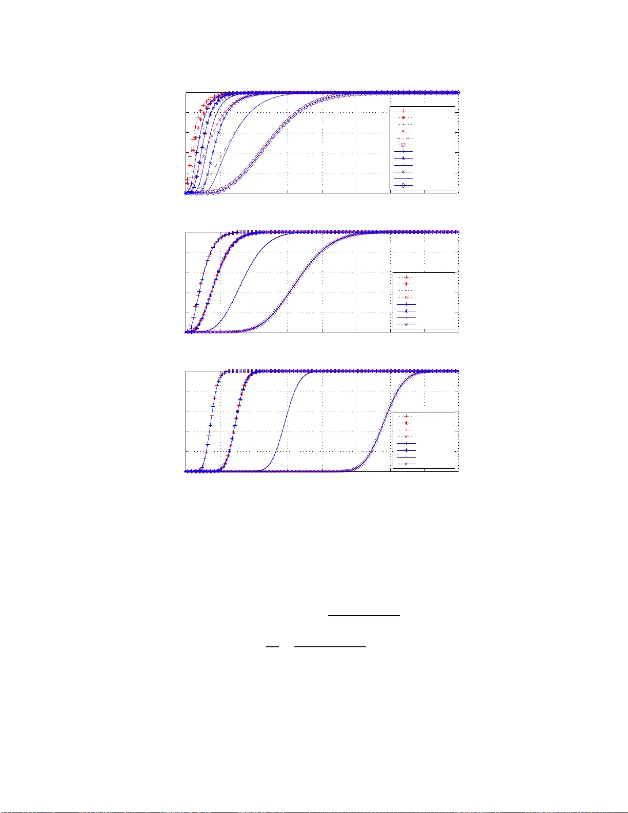
SUBMITTED TO THE IEEE TRANSA CTIONS ON INFORMA TION THEOR Y 1 Beam Selecti on Gain V ersus Antenna Selection Gain Dongwoon Bai, Saeed S. Ghass emzadeh, Robert R. M iller , and V ahid T ar okh Abstract W e consider beam selection using a fix ed beamfor ming netw ork (FBN) at a base station with M array antennas. In our setting, a Butler matrix is deployed at the RF stag e to form M beams, a nd then the best beam is selected for transmission. W e provide the pr oofs of th e key proper ties of the noncen tral chi-square distribution an d the following prop erties of the beam selection ga in verifyin g that beam selection is su perior to antenna selection in Rician ch annels with any K -factors. Furth ermore , we find asym ptotically tight stochastic bounds of the beam selectio n gain , which yield a pprox imate closed form expression s of the expected selection gain and the ergo dic capacity . Beam selection ha s the order of gr owth of the e rgodic capacity Θ (log ( M )) regardless of user location in contrast to Θ (log(lo g ( M ))) for anten na selection. I . I N T RO D U C T I O N Deploying multiple antenna s at a base station dramatically incre ases spectral efficiency . Whil e multiple- input/multiple-output (MIMO) systems requ ire multiple RF cha ins and elabo rate signa l processing un its, Antenna selection has been an attractiv e solution for multiple an tenna sy stems b ecaus e only one RF chain is required to use the ante nna with the highest signal-to-noise ratio (SNR). W ith promise of higher spectral efficiency , we focu s on beam selection ins tead o f ante nna selec tion using a FBN at a base station which deploys M multiple linear equally sp aced omnidirectional array antennas when each remote unit is equipped with an omnidirectional antenna. While the base station can adaptively steer bea ms to remote use rs using M RF chains, we in vestigate the Butler matrix, a simple FBN at the RF stag e produ cing orthogona l beams a nd requ iring only one RF chain for the best beam to be selected for trans mission [1]. The cho ice of the best beam can be achieved with pa rtial ch annel state information (CSI) at the bas e s tation. The remote feeds bac k the index of the bes t beam to the base station for the forward link. Although beam se lection has been known to have no advantage over antenna selection in ideal Rayleigh fading c hannels, it has bee n e stablished (us ing an alysis and s imulations) that bea m selec tion ca n outperform antenn a s election in correlated Rayleigh fading chann els with limit ed angle spread [2]. For the case of Rician fading cha nnels, there exist only limited analytical results of two very special case s of Rayleigh fading c hannels and deterministic cha nnels except our o wn work in [3] while simulations and measureme nts have sh own that be am selection using the Butler FBN outperforms anten na selection [4]. Moti vated by this, we have analyzed the performance of beam selection using the Butl er FBN for Rician fading c hannels with arbitrary K -factors and deriv ed the exa ct distrib ution o f the be am s election gain as a function of the azimuthal loc ation of the remo te use r in ou r p revious work [3], where some key properties This work was presented in part at the I EEE V ehicu lar T echnology Conference, Calgary , Canada, September 2008. Dongwo on Bai and V ahid T arokh are with the School of Engineering and Applied Sciences, Harvard Univ ersity , Cambridge, MA 02138, USA (email: dbai@fas.harv ard.edu; vahid@seas.harv ard.edu). Saeed S. Ghassemzadeh and Robert R. Miller are with A T&T Labs. – Research, Florham Park, NJ 07932 , USA (email: saeedg@research.att.com; rrm@research.att.com). Manuscript submitted to the IEEE Transa ctions on Information Theory on February 5, 2009. SUBMITTED TO T HE IEEE TRANSA CTIONS ON INFORMA TION THEOR Y 2 Switch Select P h y s i c a l L a y e r H i g h e r L a y e r A p p l i c a t i o n 1 2 3 4 30 60 90 270 300 330 0 Beam Pattern for M =4 Azimuthal Angle of Incident γ 1 θ γ 2 γ 3 γ 4 M × M Butler FBN ( B ) 1 y 2 y M y 1 r 2 r M r Switch Select P h y s i c a l L a y e r H i g h e r L a y e r A p p l i c a t i o n Switch Select Physical Layer Higher Layer Application 1 2 3 4 30 60 90 270 300 330 0 Beam Pattern for M =4 Azimuthal Angle of Incident γ 1 θ γ 2 γ 3 γ 4 1 2 3 4 30 60 90 270 300 330 0 Beam Pattern for M =4 Azimuthal Angle of Incident γ 1 θ γ 2 γ 3 γ 4 M × M Butler FBN ( B ) 1 y 2 y M y 1 r 2 r M r M × M Butler FBN ( B ) 1 y 2 y M y 1 y 2 y M y 1 y 2 y M y 1 r 2 r M r 1 r 2 r M r 1 r 2 r M r Fig. 1. Bea m s election sys tem u sing the Butler FBN with M linear e qually spaced array anten nas and beam pattern for M = 4 a nd d = λ c / 2 . of the non central chi-square distribution and the following properties of the b eam selec tion g ain have been pres ented without any proofs. Using thes e properties, we have compared the be am selection gain with the antenna selection ga in for Rician fading channe ls and analytically proved that beam se lection outperforms antenn a selection. In this paper , we provide the proofs omitt ed in [3], which v erify our claim t hat beam selection is superior to a ntenna selection regardles s of us er location in Rician channe ls w ith any K -factors. Moreover , w e find a symptotically tight stoch astic boun ds of the b eam s election g ain yielding approximate outage and the approximate expression for average performance. This approximation techn ique ca n be applied for most of average p erformance meas ures a s shown for the expe cted selection gain and the er godic c apacity . Using the se results, we o btain orde rs of growt h o f the expected selection gain and the ergodic c apacity for beam s election, proved to be higher than those for antenn a selection. The remainder of this p aper is organized a s follows: In Section II, we prese nt ou r system model when the Butler FBN is used in the b ase station. In Section III, we ana lyze the beam selec tion gain using a statistical a pproach. In Section IV, we compare the gain of beam selection with that of antenna selection, and prov e that bea m selection outperforms an tenna selection unde r any Rician channel transmission model. In Section V, we find s tochastic boun ds of the beam selec tion gain and approximate closed form expressions of performance mea sures. Finally , we provide our conclusions in Section VI . I I . T H E S Y S T E M M O D E L W e cons ider a bas e station endowed with M ≥ 2 anten nas (as dep icted in Fig. 1) and remote units each endowed with on e antenna. For the m -th p ort of the Butler ma trix ( m ∈ { 1 , ..., M } ), the SNR equals to ρ · Γ m regardless of the direction of the communication link [3], where ρ is the average SNR per port and Γ m denotes the gain of selecting the m -th port. This ga in is given by Γ m =   b T m h   2 , (1) where the M × 1 complex vector h = [ h 1 , ..., h M ] T represents the fla t fading channe l ga ins for corre- sponding antennas n ormalized su ch that E [ | h i | 2 ] = 1 for i = 1 , 2 , · · · , M , and the 1 × M complex vec tor SUBMITTED TO T HE IEEE TRANSA CTIONS ON INFORMA TION THEOR Y 3 b T m is the m -th row of the M × M Butler matrix gi ven by b T m = 1 √ M h e j 2 π M ( m − 1 2 ) , e j 2 π M ( m − 1 2 ) 2 , ..., e j 2 π M ( m − 1 2 ) M i . (2) Then, the base station chooses the port with the highest SNR. T o select the b est be am for the forward link, the remote use r only ne eds to feed back the index of the b est beam to the b ase station (even when the channe l is not reciprocal) and this is the only difference b etween reverse and forward link be am selection. From this po int on, we will not distinguish rev erse and forward link b eam selection in this pap er as they are analytically identical. The SNR is then gi ven by ρ · Γ ( M ) , where the no tation z ( m ) is used to de note the m -th sma llest value from any s et of finite samples { z 1 , ..., z M } , and thus Γ ( M ) = max m ∈{ 1 ,...,M } Γ m . W e de fine the beam se lection g ain as the ratio o f the S NR of b eam s election with a FBN to the av erage SNR of random antenna switching withou t a FBN, which is given by Γ ( M ) . I I I . B E A M S E L E C T I O N G A I N S I N F A D I N G C H A N N E L S It ha s been shown tha t beam s election outpe rforms antenn a selection in ide al line-of-sight (LOS) channe ls, while b eam s election performs as good as anten na selection in ide al no n-line-of-sight (NLOS) channe ls [4]. W e are interes ted in in vestigating the performance of beam selection un der Rician chan nel models. This is the mo st frequen tly used realistic ch annel mode l in wireles s communications. Under the Rician chan nel model, the no rmalized chan nel vector h can be mode led as multipath signals h = r K K + 1 h L + r 1 K + 1 h N . (3) The entries of complex vector h L (which repres ents the normalized LOS compone nt) are modeled to have unit power an d fixed pha se. The entries of the co mplex vector h N (which represe nts the normalized NLOS co mponent) are modeled by i.i.d. ind epende nt z ero-mean circularly symmetric comp lex Gaussian random variables with unit variance. The parameter K is referred to as the Rician K -factor , which represents the ratio o f the LOS s ignal power to the NLOS signal power . The spe cial cases of K = ∞ and K = 0 represe nt ideal LOS (deterministic) and ideal NLOS (Rayleigh fading) cha nnels, respectively . A. Deterministic Compon ents Consider the LOS compo nent h L . Let θ denote the az imuthal angle of incide nt betwee n a LOS s ignal and the line perpe ndicular to the li nea r equally space d array antennas assuming tw o-dimensiona l geometry (horizontal plane) as shown in Fig. 1. Furthermore, as sume tha t the distance between the base station and the mo bile us er is much larger than array antenna separation. Then for both rev erse and forward link beam se lection, h L is given by h L = exp( j ψ )  1 , exp  − j 2 π d λ c sin θ  , ..., exp  − j 2 π ( M − 1) d λ c sin θ  T , (4) where ψ is an arbitrary phase s hift of the s ignal from/to the first array anten na, d is the distance betwee n adjacen t array antennas, and λ c is the ca rrier wa velength. Let the SNR gain of the m -th beam in ideal LOS ch annels ( K = ∞ ) b e denoted by γ m ,   b T m h L   2 = ( M , if φ m = 2 π n, n ∈ Z , 1 M sin 2 ( M φ m / 2) sin 2 ( φ m / 2) , otherwise , (5) SUBMITTED TO T HE IEEE TRANSA CTIONS ON INFORMA TION THEOR Y 4 where φ m , 2 π  1 M  m − 1 2  − d λ c sin θ  . (6) Since h L is a function of θ , γ m is also a function of θ and let us call a set of M func tions { γ m | m = 1 , ..., M } a be am pattern , which has the following properties: M X m =1 γ m = M , 0 ≤ γ m ≤ M ; (7) γ m = M if and only if φ m = 2 π n M , n M ∈ Z ; (8) γ m = 0 if and only if φ m = 2 π n M , n M / ∈ Z ; (9) where the azimuthal angle s atisfying (8) is the be am dir ection . Le t us d efine a lobe of a beam as a main lobe if the beam direction is inside that lobe . W e a ssume M − 1 2 M < d λ c , (10) for all M beams to h av e at le ast one main lobe. W e examine the b eam p attern only from θ = 0 to the first bea m direction giv en by θ = ν , arcsin  1 2 M λ c d  (11) as discu ssed in [3]. B. Pr obabilistic Analysis Now , let us c onsider the statistical c hannel model includ ing NL OS c omponen ts. The cumulati ve distrib ution fun ction (cdf) o f Γ m is given by [3] F m ( x ) , Pr { Γ m ≤ x } = F χ ′ 2 (2( K + 1) x | n, δ ) | n =2 , δ =2 K γ m = E  F χ 2 (2( K + 1) x | n + 2 P δ/ 2 )    n =2 , δ =2 K γ m , (12) where F χ ′ 2 ( x | n, δ ) is the n oncentral chi-squa re cdf with n degrees o f freedom and the nonce ntrality parameter δ , P δ/ 2 is a Poisson random variable w ith mean δ / 2 , and F χ 2 ( x | q ) is the chi-square cdf with q degrees of freedom, gi ven by F χ 2 ( x | q ) = 1 − e − x/ 2 q / 2 − 1 X k =0 ( x/ 2) k k ! = e − x/ 2 ∞ X k = q / 2 ( x/ 2) k k ! (13) if q is an even numbe r as in (12 ) whe re q = n + 2 P δ/ 2 | n =2 . Note that giv en K , ev aluating γ m is enou gh to know the distributi on of the SNR gain Γ m . The beam selection gain Γ ( M ) is given by F ( M ) ( x ) , Pr { Γ ( M ) ≤ x } = M Y m =1 F m ( x ) , (14) and thus for x > 0 , log F ( M ) ( x ) = M X m =1 log F m ( x ) . (15) SUBMITTED TO T HE IEEE TRANSA CTIONS ON INFORMA TION THEOR Y 5 W e h av e the follo wing useful key theo rem o n the noncentral ch i-square distrib ution, whos e proof ca n be found in the Appe ndix. Theorem 1: The loga rithm of the noncentral chi-square cdf w ith two degrees of freedo m log F χ ′ 2 ( x | 2 , δ ) (16) is a strictly decrea sing and strictly concave function of the no ncentrality parameter δ ≥ 0 for any giv en x > 0 as suming that the ba se of logarithm is greater than o ne. Now , we are rea dy to show the following theorem, where stochas tic order relations are introduced in [5, Ch. 9]. Theorem 2: For any giv en x > 0 , F ( M ) ( x ) , the cdf of the bea m s election gain Γ ( M ) , is a strictl y decreas ing fun ction of θ from zero to the fi rst beam direction ν = arcsin  1 2 M λ c d  . Therefore, in this interval, Γ ( M ) is stochastica lly increa sing, s tochastica lly smallest at θ = 0 , and stocha stically largest at θ = ν . Pr oof: This proof is gi ven in the Ap pendix. The corollary belo w follows n aturally from Theorem 2. Cor ollary 3: For θ ∈ [ − π / 2 , π / 2] and any integer | m | ≤ M λ c /d , Γ ( M ) is stoch astically increas ing as θ increases if θ ∈  arcsin  m M λ c d  , arcsin  min  m + 1 / 2 M λ c d , 1  , (17) and stoch astically decreasing as θ increases if θ ∈  arcsin  max  m − 1 / 2 M λ c d , − 1  , arcsin  m M λ c d  . (18) It is exac tly opposite for the other half of the horizon tal plane, θ ∈ [ π / 2 , 3 π / 2] . Therefore, Γ ( M ) with θ = 0 and θ = ν are achiev able stoch astic lo wer and up per b ounds, respectiv ely for Γ ( M ) with an arbitrary θ . Corollary 3 tells u s that the expe cted pe rformance measures over Γ ( M ) with θ = 0 and θ = ν can serve as lower and upper bounds , resp ectiv ely , for the a verages of a ny pe rformance measures which are increasing func tions of SNR, e.g ., the channel ca pacity . They can a lso se rve as uppe r and lo wer bo unds, respectively , for the averages of any performance measures which are decreas ing functions of SNR, e.g ., the bit e rror rate (BER), applying the res ult in [5, pp . 405 –406]. I V . B E A M S E L E C T I O N V E R S U S A N T E N N A S E L E C T I O N Let us co nsider the an tenna selection gain under the same scena rio use d for beam selec tion case except the fact that the Butler F BN will not be deployed for antenn a selection. When the m -th an tenna is s elected among M antennas in the base station, the SNR is giv en by ρ · H m , where H m , | h m | 2 . As suming that the anten na with the highest SNR is always se lected, the an tenna selection gain is de fined as the ratio of the SNR of an tenna selec tion to the av erage SNR o f rand om antenna s witching, which c an be expressed by H ( M ) . For any m , the cdf of H m becomes G ( x ) , Pr { H m ≤ x } = F χ ′ 2 (2( K + 1) x | 2 , 2 K ) . (19) SUBMITTED TO T HE IEEE TRANSA CTIONS ON INFORMA TION THEOR Y 6 Therefore, the cd f of H ( M ) is given by G ( M ) ( x ) , Pr { H ( M ) ≤ x } = G M ( x ) . (20) W ith the proofs of previous theorems , we can c onfirm that the follo wing lemma holds. Lemma 1: For the same Rician K -factor , beam selection always outperforms anten na selection, i.e ., the be am selection gain Γ ( M ) is stochas tically lar ger tha n the a ntenna selection gain H ( M ) . Pr oof: Applying the con cavity resu lt in The orem 1 and J ensen ’ s ine quality giv es us log G ( M ) ( x ) = M log F χ ′ 2 (2( K + 1) x | 2 , 2 K ) ≥ M X m =1 log F χ ′ 2 (2( K + 1) x | 2 , 2 K γ m ) = log F ( M ) ( x ) , (21) for any given x > 0 . V . A S Y M P T O T I C S E L E C T I O N G A I N S It has been shown that the be am selection gain is stochastically u pper and lo wer boun ded b y Γ ( M ) with θ of z ero and the first b eam direction ν = arcsin  1 2 M λ c d  , respectively . Our interest in this section is to s ee how these two extremes change a s the nu mber o f antennas M increase s and then obtain the asymptotic se lection ga in for a n a rbitrary location of the remo te use r . F urthermore, thes e analytica l results can be ap plied to study the outage and the ergodic c apacity of b eam selection systems . For this purpose, consider the S NR gain Γ m ( θ ) an d its cdf F m ( ·| θ ) as functions of the azimuthal angle θ . A. Bounds and Appr o ximations First, we can obtain the stocha stic lower b ound for the bea m selection gain of the use r at the beam direction Γ ( M ) ( ν ) given by F ( M ) ( x | ν ) = M Y m =1 F χ ′ 2 (2( K + 1) x | 2 , 2 K γ m ( ν )) = F χ ′ 2 (2( K + 1) x | 2 , 2 K M ) · F M − 1 χ 2 (2( K + 1) x | 2) = Q M ( x ) W M − 1 ( x ) ≤ Q M ( x ) , (22) where Q and W are defined by Q γ ( x ) , F χ ′ 2 (2( K + 1) x | 2 , 2 K γ ) , (23) W ( x ) , F χ 2 (2( K + 1) x | 2) . (24) Fig. 2 shows F ( M ) ( x | ν ) and its stoc hastic lower b ound Q M . It can be se en that the lower boun d Q M approach es to the cdf F ( M ) ( x | ν ) a s M increases, which will be proved. Now , cons ider the beam selection ga in of the user exactly between beams Γ ( M ) (0) and its cd f given by F ( M ) ( x | 0) = M Y m =1 F χ ′ 2 (2( K + 1) x | 2 , 2 K γ m (0)) . (25) SUBMITTED TO T HE IEEE TRANSA CTIONS ON INFORMA TION THEOR Y 7 0 5 10 15 20 25 30 35 40 0 0.2 0.4 0.6 0.8 1 Selection Gain Pr(Selection Gain < Abscissa) K = −10 dB, θ = ν 0 5 10 15 20 25 30 35 40 0 0.2 0.4 0.6 0.8 1 Selection Gain Pr(Selection Gain < Abscissa) K = 0 dB, θ = ν 0 5 10 15 20 25 30 35 40 0 0.2 0.4 0.6 0.8 1 Selection Gain Pr(Selection Gain < Abscissa) K = 10 dB, θ = ν L.B. : M = 4 L.B. : M = 8 L.B. : M = 16 L.B. : M = 32 L.B. : M = 64 L.B. : M = 128 Exact : M = 4 Exact : M = 8 Exact : M = 16 Exact : M = 32 Exact : M = 64 Exact : M = 128 L.B. : M = 4 L.B. : M = 8 L.B. : M = 16 L.B. : M = 32 Exact : M = 4 Exact : M = 8 Exact : M = 16 Exact : M = 32 L.B. : M = 4 L.B. : M = 8 L.B. : M = 16 L.B. : M = 32 Exact : M = 4 Exact : M = 8 Exact : M = 16 Exact : M = 32 Fig. 2 . Distributi ons of the be am selec tion gain Γ ( M ) ( ν ) a nd its stocha stic lo wer bound for K = − 10 , 0 , 10 dB, where d = λ c / 2 is assumed. Let us choose a vector u = [ u (1) , ..., u ( M ) ] which majorize s the b eam pattern { γ m (0) | m = 1 , ..., M } as γ 1 (0) = γ M (0) = u ( M ) = u ( M − 1) = 1 M sin 2 ( π / 2 M ) , a M > u ( M − 2) = u ( M − 3) = M 2 − 1 M sin 2 ( π / 2 M ) , b M > γ 2 (0) = γ M − 1 (0) > γ 3 (0) , ..., γ M − 2 (0) > u ( M − 4) = ... = u (1) = 0 , (26) where majorization is introduced in [6, p. 45]. SUBMITTED TO T HE IEEE TRANSA CTIONS ON INFORMA TION THEOR Y 8 Notation: For any two real-valued sequenc es c M and d M , we define c M ≈ d M if and only if lim M → ∞ | c M − d M | = 0; c M ∼ d M if and only if lim M → ∞ c M /d M = 1; c M = Θ ( d M ) if and only if 0 < lim M → ∞ c M /d M < ∞ . Using this n otation, we c an see a M ∼ 4 π 2 M = (0 . 4053 ... ) × M , (27) b M ∼  1 2 − 4 π 2  M = (0 . 0947 ... ) × M . (28) Applying Ha rdy-Little wood-P ´ olyas theorem in [6, pp. 88–9 1] and the strict co ncavity o f (16) to (25) yields the stochastic upper boun d F ( M ) ( x | 0) ≥ M Y m =1 F χ ′ 2 (2( K + 1) x | 2 , 2 K u ( m ) ) = F 2 χ ′ 2 (2( K + 1) x | 2 , 2 K a M ) · F 2 χ ′ 2 (2( K + 1) x | 2 , 2 K b M ) · F M − 4 χ 2 (2( K + 1) x | 2) = Q 2 a M ( x ) · Q 2 b M ( x ) · W M − 4 ( x ) . (29) Thus, we ha ve the stoch astic lo wer and u pper bound for F ( M ) ( x | 0) g i ven by Q 2 a M ( x ) ≥ F ( M ) ( x | 0) ≥ Q 2 a M ( x ) · Q 2 b M ( x ) · W M − 4 ( x ) . (30) Fig. 3 shows F ( M ) ( x | 0) and its stoch astic lo wer bou nd Q 2 a M and u pper bound Q 2 a M Q 2 b M W M − 4 . W e also obse rve that as the lower and upper bounds are merged into eac h other , so does F ( M ) ( x | 0) as M increases . The following theorem verifies tha t the stoc hastic lower bounds in (22) and (30) are inde ed asymptot- ically tight. Theorem 4: For K > 0 and p ∈ [0 , 1) , F − 1 ( M ) ( p | ν ) ≈ Q − 1 M ( p ) (31) and F − 1 ( M ) ( p | 0) ≈ Q − 1 a M ( √ p ) (32) as M increases . Pr oof: This proof is gi ven in the Ap pendix. W e also have the follo wing theo rem use ful for average pe rformance ev aluation, whose proof can be found in the Appendix. Theorem 5: Let h be any differentiable function defined on [0 , ∞ ) suc h that h ′ is bounde d. If h is integrable with respec t to Q M , then Z ∞ 0 h ( x ) dF ( M ) ( x | ν ) ≈ Z ∞ 0 h ( x ) dQ M ( x ) (33) as M increases . If h is integrable with re spect to Q 2 a M , then Z ∞ 0 h ( x ) dF ( M ) ( x | 0) ≈ Z ∞ 0 h ( x ) dQ 2 a M ( x ) (34) as M increases . SUBMITTED TO T HE IEEE TRANSA CTIONS ON INFORMA TION THEOR Y 9 0 5 10 15 20 25 0 0.2 0.4 0.6 0.8 1 Selection Gain Pr(Selection Gain < Abscissa) K = −10 dB, θ = 0 0 5 10 15 20 25 0 0.2 0.4 0.6 0.8 1 Selection Gain Pr(Selection Gain < Abscissa) K = 0 dB, θ = 0 0 5 10 15 20 25 0 0.2 0.4 0.6 0.8 1 Selection Gain Pr(Selection Gain < Abscissa) K = 10 dB, θ = 0 U.B. : M = 4 U.B. : M = 16 U.B. : M = 64 U.B. : M = 256 L.B. : M = 4 L.B. : M = 16 L.B. : M = 64 L.B. : M = 256 Exact : M = 4 Exact : M = 16 Exact : M = 64 Exact : M = 256 U.B. : M = 4 U.B. : M = 8 U.B. : M = 16 U.B. : M = 32 L.B. : M = 4 L.B. : M = 8 L.B. : M = 16 L.B. : M = 32 Exact : M = 4 Exact : M = 8 Exact : M = 16 Exact : M = 32 U.B. : M = 4 U.B. : M = 8 U.B. : M = 16 U.B. : M = 32 L.B. : M = 4 L.B. : M = 8 L.B. : M = 16 L.B. : M = 32 Exact : M = 4 Exact : M = 8 Exact : M = 16 Exact : M = 32 Fig. 3. Distrib utions of the beam selection gain Γ ( M ) (0) and its stochastic lower and upper bounds for K = − 10 , 0 , 10 dB, where d = λ c / 2 is assumed. Theorems 4 and 5 in this su bsection d emonstrate that for large M , the distributions of the beam selection gain of the use r at the be am direction Γ ( M ) ( ν ) a nd the bea m selec tion gain o f the user exactly between be ams Γ ( M ) (0) c an b e well app roximated by Q M ( x ) an d Q 2 a M ( x ) , respectiv ely , which are the noncen tral chi-square distributi on and its square. The se are use ful as the ir closed-form expres sions are complicated and thus not insightful. SUBMITTED TO T HE IEEE TRANSA CTIONS ON INFORMA TION THEOR Y 10 B. P erformance Analysis It can be se en that outage probabilities with θ = 0 and θ = ν for a given rate C 0 can be approximated by P out ( C 0 ) , Pr  log 2  1 + ρ Γ ( M ) ( θ )  ≤ C 0  ≈    Q M  2 C 0 − 1 ρ  , if θ = ν , Q 2 a M  2 C 0 − 1 ρ  , if θ = 0 , (35) for lar ge M . Furthermore, Theorem 4 can be use d to approx imate outage cap acities with θ = 0 a nd θ = ν as C out ( P 0 ) , P − 1 out ( P 0 ) = log 2 h 1 + ρF − 1 ( M ) ( P 0 | θ ) i ≈  log 2  1 + ρQ − 1 M ( P 0 )  , if θ = ν, log 2  1 + ρQ − 1 a M ( √ P 0 )  , if θ = 0 . (36) for large M . Let us apply Theore m 5 to the mean s election gain E  Γ ( M )  by taking h ( x ) = x . The expe cted b eam selection ga in for θ = ν is g i ven by E  Γ ( M ) ( ν )  ≈ Z ∞ 0 xdQ M ( x ) = K M + 1 K + 1 = Θ ( M ) . (37) The expecte d bea m selection ga in for θ = 0 is giv en by E  Γ ( M ) (0)  ≈ Z ∞ 0 xdQ 2 a M ( x ) , (38) as M increase s. Although it s eems dif ficult to solve the integration in (38), we ca n obtain uppe r and lower boun ds using an ine quality in [7, p. 6 2] bec ause Q 2 a M is the cd f of the maximum of two samples from Q a M , whos e mean and variance a re ( K a M + 1) / ( K + 1) and (2 K a M + 1) / ( K + 1) 2 , respe cti vely . These boun ds are giv en by K a M + 1 K + 1 ≤ Z ∞ 0 xdQ 2 a M ( x ) ≤ K a M + 1 K + 1 + 1 √ 3 √ 2 K a M + 1 K + 1 , (39) which yields E  Γ ( M ) (0)  ≈ Z ∞ 0 xdQ 2 a M ( x ) ∼ K a M + 1 K + 1 = Θ ( M ) (40) Hence, E  Γ ( M )  = Θ ( M ) regardless of u ser location, which is f aster than Θ (log M ) for anten na selection [8]. Lemma 2: Le t ρ > 0 denote SNR. As M increases, the e r godic capacity of the user at the beam direction ( θ = ν ) is g i ven by E  log 2  1 + ρ Γ ( M ) ( ν )  ≈ log 2  1 + ρ K M + 1 K + 1  , (41) and the ergodic c apacity of the us er exactly between bea ms ( θ = 0 ) is given by E  log 2  1 + ρ Γ ( M ) (0)  ≈ log 2  1 + ρ K a M + 1 K + 1  . (42) Pr oof: This proof is gi ven in the Ap pendix. SUBMITTED TO T HE IEEE TRANSA CTIONS ON INFORMA TION THEOR Y 11 5 10 15 20 25 30 0 1 2 3 4 5 6 M Ergodic Capacity (bits/channel use) K = 0 dB, ρ = 5 dB Exact, θ = ν Appr., θ = ν Exact, θ = 0 Appr., θ = 0 Fig. 4. E r godic capacity versus M for K = 0 dB at ρ = 5 dB , where d = λ c / 2 is assumed. This lemma also yields the order of growth of the ergodic capacity E  log 2  1 + ρ Γ ( M )  ≈ Θ (log ( M )) regardless of us er loc ation, which is faster than Θ (log (log ( M ))) for antenna s election [8]. Fig. 4 s hows the ergodic capacity and its approximations in (41) a nd (42) for S NR ρ = 5 dB. W e see that the approximations approa ch the numerically inte grated exact values as M increases. V I . C O N C L U S I O N W e considered bea m selection using the Butler FBN at the base station with multiple linear equally space d o mnidirectional array antenn as. Completing the analysis of the be am selec tion gain, we provided the proofs of the key p roperties verifying that be am s election is supe rior to a ntenna selection in Rician channe ls with any K -factors. W e also foun d asymptotically tight stochas tic b ounds of the beam selection gain and ap proximate closed form expression s of the expected selection gain and the er godic ca pacity . Using thes e results, it was shown that beam selection has high er order o f growth of the er godic capacity than antenna selection. Graphical results were pro vided demons trating the underlying gains a nd supporting our app roximations. SUBMITTED TO T HE IEEE TRANSA CTIONS ON INFORMA TION THEOR Y 12 A P P E N D I X Pr oof of Theorem 1: W ithout loss of generality , assume the natural logarithm. For any given x > 0 , (16) can be expressed as log F χ ′ 2 ( x | 2 , δ ) = log " ∞ X i =0 e − δ/ 2 ( δ / 2) i i ! α i # = − δ 2 + log " ∞ X i =0 ( δ / 2) i i ! α i # , (43) where α i is defi ned as α i , F χ 2 ( x | 2 + 2 i ) = e − x/ 2 ∞ X k = i +1 ( x/ 2) k k ! (44) from (13). Differentiating (43) gives us ∂ ∂ δ log F χ ′ 2 ( x | 2 , δ ) = − 1 2 + 1 2 · P ∞ i =0 ( δ/ 2) i i ! α i +1 P ∞ i =0 ( δ/ 2) i i ! α i = P ∞ i =0 ( δ/ 2) i i ! ( α i +1 − α i ) 2 P ∞ i =0 ( δ/ 2) i i ! α i < 0 (45) for δ > 0 because α i +1 < α i from (44), an d thus (16) is a strictly decreasing function of δ ≥ 0 . Now , prove that (16) is a strictly c oncave function of δ ≥ 0 . The second deri vati ve of (43) is given by ∂ 2 ∂ δ 2 log F χ ′ 2 ( x | 2 , δ ) =  P ∞ i =0 ( δ/ 2) i i ! α i   P ∞ i =0 ( δ/ 2) i i ! α i +2  −  P ∞ i =0 ( δ/ 2) i i ! α i +1  2 4  P ∞ i =0 ( δ/ 2) i i ! α i  2 , (46) the i -th orde r term of whose numerator ca n be simplified a s ( δ / 2) i i ! ( α 0 α i +2 − α 1 α i +1 ) . (47) Let u s sh ow that (46) is negative by proving that (47) is n egati ve for δ > 0 . Conside r α i − 1 /α i , wh ich is an increas ing fun ction of i becaus e α i − 1 α i − 1 = ( x/ 2) i i ! P ∞ k = i +1 ( x/ 2) k k ! = 1 P ∞ k =1 ( x/ 2) k ( i + k )! /i ! (48) and ( i + k )! /i ! increases as i inc reases for any po siti ve integer k . Therefore, α 0 α 1 < α 1 α 2 < ... < α i +1 α i +2 < ..., (49) which yields the strict concavity of (16). Pr oof of Theo r em 2: Define β , 2 π d λ c sin θ . (50) SUBMITTED TO T HE IEEE TRANSA CTIONS ON INFORMA TION THEOR Y 13 Under the cond ition (10), β is an increasing an d co ntinuous function o f θ and has the range  0 , π M  . Therefore, we only need to show that F ( m ) is a strictly decrea sing func tion of β in the domain  0 , π M  . From (6), φ m ( β ) , 2 π M  m − 1 2  − β = φ m (0) − β , ( 51) and by d efining η ( φ ) = ( M if φ = 2 π n, n ∈ N 1 M sin 2 ( M φ/ 2) sin 2 ( φ/ 2) otherwise , (52) we can rep resent γ m ( β ) = η ( φ m ( β )) . (53) Note that η ( φ ) is a periodic function with period 2 π , symme tric with respect to the axis φ = π n , an d the value of η at φ = 2 π n makes η ( φ ) a continuou s function of φ . First, p rove that for β ∈  0 , π M  the be am pattern { γ m } ca n be sorted in noninc reasing order a s follows: γ 1 ( β ) ≥ γ M ( β ) ≥ γ 2 ( β ) ≥ γ M − 1 ( β ) ≥ ... ≥ γ ⌊ M 2 ⌋ +1 ( β ) , (54) where ⌊·⌋ is a floor fun ction. It c an be ea sily shown that γ M +1 − m ( β ) = η ( φ m ( − β )) = γ m ( − β ) . (55) W e g et the follo wing equiv alent inequalities of (54) η ( φ 1 ( β )) ≥ η ( φ 1 ( − β )) ≥ ... ≥ η  φ ⌊ M +1 2 ⌋  ( − 1) M − 1 β   . (56) W e c an see that η ( φ m ( ± β )) = 1 M sin 2  M 2 φ m ( ± β )  sin 2  1 2 φ m ( ± β )  = 1 M cos 2  M 2 β  sin 2  1 2 φ m ( ± β )  (57) and 0 ≤ φ 1 ( β ) ≤ φ 1 ( − β ) ≤ ... ≤ φ ⌊ M +1 2 ⌋  ( − 1) M − 1 β  ≤ π , (58) which y ields (56) becaus e in (57), the nume rator sin 2  M 2 φ  has the same value a t φ = φ m ( ± β ) for any fixed β and all m , a nd the denominator s in 2  1 2 φ  is inc reasing function of φ ∈ [0 , π ] . De fine the nondec reasingly sorted vector γ from { γ m } given by γ , [ γ (1) , γ (2) , ..., γ ( M ) ] = h γ ⌊ M 2 ⌋ +1 , ..., γ M − 1 , γ 2 , γ M , γ 1 i (59) for β ∈  0 , π M  . Let us show that γ ( β 2 ) strictly ma jorizes γ ( β 1 ) for 0 ≤ β 1 < β 2 ≤ π M , which me ans M X i =1 γ ( i ) ( β 1 ) = M X i =1 γ ( i ) ( β 2 ) ( 60) and m X i =1 γ ( i ) ( β 1 ) > m X i =1 γ ( i ) ( β 2 ) ( 61) SUBMITTED TO T HE IEEE TRANSA CTIONS ON INFORMA TION THEOR Y 14 for all m ∈ { 1 , ..., M − 1 } . W e already hav e (60) from (7), a nd thus it suffices to prove (61). U nder the assumption that (61) is proved, using Hardy-Little wood-P ´ olyas theorem in [6, pp. 88–91] based on the strict co ncavity of (16) proved in Th eorem 1 gives us log F ( M ) ( x | K, β 1 ) = M X m =1 log F χ ′ 2 (2( K + 1) x | 2 , 2 K γ m ( β 1 )) > M X m =1 log F χ ′ 2 (2( K + 1) x | 2 , 2 K γ m ( β 2 )) = log F ( M ) ( x | K, β 2 ) , (62) which bas ically shows that F ( m ) is a strictly decreasing function of β . Let u s prove that γ 1 ( β ) and γ M ( β ) are strictly increasing a nd strictly decreasing respectively . For φ 6 = 2 π n , it c an be s hown that η ′ ( φ ) = 1 M sin 2  M 2 φ  sin 2  1 2 φ   M cot  M 2 φ  − cot  1 2 φ  . (63) W e c an show η ′ ( φ ) is negati ve for 0 < φ < 2 π M becaus e by the T aylor series expans ion, M cot  M 2 φ  − cot  1 2 φ  = M " 2 M φ − ∞ X i =1 2 2 i | B 2 i | (2 i )!  M 2 φ  2 i − 1 # − " 2 φ − ∞ X i =1 2 2 i | B 2 i | (2 i )!  1 2 φ  2 i − 1 # = − ∞ X i =1 2 2 i | B 2 i | (2 i )! ( M 2 i − 1)  φ 2  2 i − 1 < 0 (64) where B i is the i -th Bernoulli number . The refore, η ( φ ) is strictly d ecreasing in  0 , 2 π M  , a nd thus η ( φ ) is strictly increa sing in  2 π M − 1 M , 2 π  by the symmetry . Since γ 1 ( β ) = η  π M − β  (65) and γ M ( β ) = η  2 π M − 1 / 2 M − β  , (66) we have p roved our claim. Now , con sider the case when M ≥ 3 and m = 2 , ..., M − 1 . W e can see that if m < ( M + 1) / 2 , γ M +1 − m ( β ) is strictly dec reasing becau se the numerator and the d enominator in (52) are strictly de- creasing and strictly increasing respectiv ely as func tions of β . Moreover , we c an show the fact that γ m ( β ) + γ M +1 − m ( β ) is strictly de creasing, which can lea d to the consequ ence that γ M +1 2 ( β ) is strictly decreas ing for odd M and thus γ M +1 − m ( β ) is s trictly d ecreasing for m = ( M + 1) / 2 as well. It suffices to prove tha t γ ′ m ( β ) + γ ′ M +1 − m ( β ) < 0 (67) for β ∈  0 , π M  . From (55), γ m ( β ) + γ M +1 − m ( β ) = 1 M sin 2 ( M φ m ( β ) / 2 ) sin 2 ( φ m ( β ) / 2 ) + 1 M sin 2 ( M φ m ( − β ) / 2) sin 2 ( φ m ( − β ) / 2) = 1 M cos 2  M 2 β   csc 2 ( φ m ( β ) / 2 ) + csc 2 ( φ m ( − β ) / 2)  , (68) SUBMITTED TO T HE IEEE TRANSA CTIONS ON INFORMA TION THEOR Y 15 becaus e it can be sh own that sin 2 ( M φ m ( β ) / 2 ) = sin 2 ( M φ m ( − β ) / 2) = cos 2  M 2 β  . (69) By de fining f ( β ) , cos 2  M 2 β  , (70) g 1 ( β ) , csc 2 ( φ m ( β ) / 2 ) , g 2 ( β ) , csc 2 ( φ m ( − β ) / 2) , (71) we have the expression γ ′ m + γ ′ M +1 − m = 1 M f ( g 1 + g 2 )  f ′ f + g ′ 1 + g ′ 2 g 1 + g 2  . (72) Since f > 0 and g 1 + g 2 > 0 for β ∈  0 , π M  , we on ly need to show h , f ′ f + g ′ 1 + g ′ 2 g 1 + g 2 < 0 . (73) Simple deriv ations giv e us f ′ f = − M tan  M 2 β  , (74) g ′ 1 = d dβ  csc 2  φ m ( β ) 2  = csc 2  φ m ( β ) 2  cot  φ m ( β ) 2  , (75) and similarly g ′ 2 = − csc 2  φ m ( − β ) 2  cot  φ m ( − β ) 2  . (76) W e g et h ( β ) = − M tan  M 2 β  + csc 2  φ m ( β ) 2  cot  φ m ( β ) 2  − csc 2  φ m ( − β ) 2  cot  φ m ( − β ) 2  csc 2  φ m ( β ) 2  + csc 2  φ m ( − β ) 2  . (77 ) Becaus e 0 < φ m ( β ) / 2 , φ m ( − β ) / 2 < π , applying the me an value theorem yields csc 2  φ m ( β ) 2  cot  φ m ( β ) 2  − csc 2  φ m ( − β ) 2  cot  φ m ( − β ) 2  − β = − 2 csc 2 ψ cot 2 ψ − csc 4 ψ . (78) for some ψ ∈ ( φ m ( β ) / 2 , φ m ( − β ) / 2) . Then , h ( β ) = − M tan  M 2 β  + β csc 4 ψ (2 cos 2 ψ + 1) csc 2  φ m ( β ) 2  + csc 2  φ m ( − β ) 2  . (79) SUBMITTED TO T HE IEEE TRANSA CTIONS ON INFORMA TION THEOR Y 16 W e can see that for ψ ∈ [ φ m ( β ) / 2 , φ m ( − β ) / 2] , csc 4 ψ (2 cos 2 ψ + 1) has maximum at eit her ψ = φ m ( β ) / 2 or ψ = φ m ( − β ) / 2 and let it b e denoted by ψ b . W e a re ready to show the followi ng se ries of inequalities h ( β ) < − M tan  M 2 β  + β csc 4 ψ b (2 cos 2 ψ b + 1) csc 2 ψ b + 1 < − M 2 2 β + β csc 2 ψ b  − 2 + 10 3 − cos 2 ψ b  < − M 2 2 β + 3 β csc 2 ψ b < − M 2 2 β + 3 β 1 sin 2 π M < M 2 2 β    − 1 + 6 π 2 n 1 − 1 6  π M  2 o 2    < 0 , (80) where the last ine quality ho lds as M ≥ 3 . This proves (73), and thus (67) follows. It is clear that P m i =1 γ ( i ) ( β ) is s trictly decreasing for a ll m ∈ { 1 , ..., M − 1 } be cause γ M +1 − m ( β ) (81) and γ m ( β ) + γ M +1 − m ( β ) (82) are strictly decreas ing for m = 1 , ..., ⌊ M +1 2 ⌋ , which we has been proved a bove, a nd P m i =1 γ ( i ) ( β ) bec omes either the sum of (82) for multiple m or the s um of (81) and (82 ) for multiple m . Th e v alidity o f (62) completes our p roof. Pr oof of Theorem 4: All functions in (31) and (32) take the value 0 if a nd only if x = 0 . Thus, we can as sume p ∈ (0 , 1) . T o sh ow (31), define x 1 , Q − 1 M ( p ) and x 2 , F − 1 ( M ) ( p | ν ) and this yields Q M ( x 1 ) = Q M ( x 2 ) W M − 1 ( x 2 ) = p. (83) Let us introduce a new variable x 3 to obtain upper bound for x 2 giv en by x 3 , Q − 1 M  p W M − 1 ( x 1 )  ≥ x 2 ≥ x 1 . (84 ) Let us show x 3 ≈ x 1 , and then x 2 ≈ x 1 in (31) follows immediately . The value of x 1 can be c omputed using Sankaran’ s approximation in [9], where it has been sugge sted that for a random v ariable X with the cd f F χ ′ 2 ( x | n, δ ) , { X − ( n − 1) / 2 } 1 / 2 − { δ + ( n − 1) / 2 } 1 / 2 is app roximately ze ro mean Ga ussian with unit variance and this approximation improves if either n or δ increase s. Thu s as M increase s, x 1 ≈ 1 2( K + 1)   1 2 + (  2 K M + 1 2  1 2 + Φ − 1 ( p ) ) 2   ∼ K K + 1 M , (85) where Φ − 1 is the in verse function of the Gauss ian cdf giv en by Φ( x ) = 1 √ 2 π Z x −∞ e − t 2 2 dt. (86) SUBMITTED TO T HE IEEE TRANSA CTIONS ON INFORMA TION THEOR Y 17 Let us us e the no tations µ F and σ 2 F to d enote the mean and variance of distributi on F , respectively . Then, it c an be s hown that µ W M − 1 ≈ q M − 1 + ζ 2( K + 1) , σ 2 W M − 1 ≈ π 2 / 6 { 2( K + 1) } 2 , (87) where q M − 1 , W − 1 (1 − 1 / ( M − 1)) ≈ ln( M − 1) and ζ , 0 . 5772 ... (Eu ler’ s constan t) [8]. For x 1 > µ W M − 1 (this is true for all M > C for some C ), applying one-sided Chebyshev’ s inequality in [10, p. 152] yields 1 − W M − 1 ( x 1 ) ≤ 1 1 + ( x 1 − µ W M − 1 ) 2 /σ 2 W M − 1 , (88) and thus 1 ≤ 1 W M − 1 ( x 1 ) ≤ 1 + ǫ M , (89) where 0 < ǫ M , σ 2 W M − 1 ( x 1 − µ W M − 1 ) 2 ∼ π 2 24 1 K 2 M 2 (90) by (85) an d (87) as M increa ses. W e have x 3 − x 1 ≤ Q − 1 M ( p (1 + ǫ M )) − Q − 1 M ( p ) ≈ 1 K + 1  2 K M + 1 2  1 2  Φ − 1 ( p (1 + ǫ M )) − Φ − 1 ( p )  + 1 2( K + 1) h  Φ − 1 ( p (1 + ǫ M ))  2 −  Φ − 1 ( p )  2 i ≈ 1 K + 1  2 K M + 1 2  1 2 ǫ M p 1 Φ ′ (Φ − 1 ( p (1 + ε ))) , ε ∈ (1 , ǫ M ) ≈ 0 , (91) as M increase s, becau se (2 K M + 1 / 2) 1 / 2 · ǫ M ≈ 0 from (90 ). Hence, (31) is proved. Now , (32) can be shown similarly . For any p ∈ (0 , 1) , let us define x 4 , Q − 1 a M ( √ p ) and x 5 as Q 2 a M ( x 5 ) · Q 2 b M ( x 5 ) · W M − 4 ( x 5 ) = p (92) From (30), defining x 6 yields x 6 , Q − 1 a M √ p Q b M ( x 4 ) W M − 4 2 ( x 4 ) ! ≥ x 5 ≥ F − 1 ( M ) ( p | 0) ≥ x 4 . (93) Assuming x 6 ≈ x 4 , we hav e F − 1 ( M ) ( p | 0) ≈ x 4 in (32). N ow , as M increas es, it can b e shown tha t x 4 ∼ K K + 1 a M (94) SUBMITTED TO T HE IEEE TRANSA CTIONS ON INFORMA TION THEOR Y 18 as above. Note that Q b M W M − 4 2 is the d istrib ution of the maximum of two inde penden t rando m vari ables follo wing Q b M and W M − 4 2 . It can be ea sily proved that µ Q b M W M − 4 2 ≤ µ Q b M + µ W M − 4 2 ≈ K b M + 1 K + 1 + q M − 4 2 + ζ 2( K + 1) ∼ K K + 1 b M (95) and σ 2 Q b M W M − 4 2 ≤ σ 2 Q b M + σ 2 W M − 4 2 +  µ W M − 4 2  2 ≈ K b M + 1 ( K + 1) 2 + π 2 / 6 { 2( K + 1) } 2 + q M − 4 2 + ζ 2( K + 1) ! 2 ∼ K ( K + 1) 2 b M . (96) Once ag ain u sing one -sided Chebyshev’ s ineq uality , 1 ≤ 1 Q b M ( x 4 ) W M − 4 2 ( x 4 ) ≤ 1 + ǫ ′ M , (97) where 0 < ǫ ′ M , σ 2 Q b M W M − 4 2  x 4 − µ Q b M W M − 4 2  2 ∼ 1 K 1 / 2 − 4 /π 2 (8 /π 2 − 1 / 2) 2 1 M = (0 . 9820 ... ) × 1 K M , (98) As M increases, this implies (2 K a M + 1 / 2) 1 / 2 · ǫ ′ M ≈ 0 , which lea ds us x 6 ≈ x 4 as in (91 ). Pr oof of Theorem 5: Let us sho w (33), first. Le t X F denote a rand om variable follo wing any distrib ution F . Obviously , Γ ( M ) ( ν ) is stocha stically lar ger than X Q M from (22). Using the idea of c oupling [5, Sec . 9.2], defin e Γ ∗ ( M ) ( ν ) , F − 1 ( M ) ( Q M ( X Q M ) | ν ) . (99) Then, Γ ( M ) ( ν ) and Γ ∗ ( M ) ( ν ) share the sa me distribution but Γ ∗ ( M ) ( ν ) ≥ X Q M with probability 1 . By the mean value theorem, we h av e h ( Γ ∗ ( M ) ( ν )) − h ( X Q M ) = h ′ ( ε ) h Γ ∗ ( M ) ( ν ) − X Q M i , (100) SUBMITTED TO T HE IEEE TRANSA CTIONS ON INFORMA TION THEOR Y 19 for some ε ∈  X Q M , Γ ∗ ( M ) ( ν )  . Using this,   E  h ( Γ ( M ) ( ν )) − h ( X Q M )    =    E h h ( Γ ∗ ( M ) ( ν )) − h ( X Q M ) i    ≤ E h    h ( Γ ∗ ( M ) ( ν )) − h ( X Q M )    i ≤ C · E h    Γ ∗ ( M ) ( ν ) − X Q M    i = C ·   E  Γ ( M ) ( ν ) − X Q M    , (101) where | h ′ | is b ounded by C . Now , let us s how E  Γ ( M ) ( ν )  ≈ E [ X Q M ] . For any x ≥ 0 , Q M ( x ) ≥ F ( M ) ( x | ν ) = Q M ( x ) W M − 1 ( x ) ≥  Q M ( x ) + W M − 1 ( x ) − 1  + , (102) where [ · ] + is defi ned as [ y ] + ,  y if y ≥ 0 , 0 if y < 0 . (103) As Q M + W M − 1 − 1 is an increasing and con tinuous fun ction of [0 , ∞ ) on to [ − 1 , 1) , there exists only one α ≥ 0 such that Q M ( α ) + W M − 1 ( α ) − 1 = 0 . (104) Therefore, 0 ≤ E  Γ ( M ) ( ν ) − X Q M  = Z ∞ 0  1 − F ( M ) ( x | ν )  − (1 − Q M ( x ))  d x ≤ Z ∞ 0 h Q M ( x ) −  Q M ( x ) + W M − 1 ( x ) − 1  + i d x = Z α 0 Q M ( x ) d x + Z ∞ α  1 − W M − 1 ( x )  d x ≤ Z β 0 Q M ( x ) d x + Z ∞ β  1 − W M − 1 ( x )  d x (105 ) for any β ≥ 0 a s (105) can be minimized by ch oosing β = α . Let us obtain the upp er bound for the first term of (105 ) using the Marcum Q-function de fined and boun ded as Ψ( a, b ) , Z ∞ b xe ( x 2 + a 2 ) / 2 I 0 ( ax ) d x ≥ 1 − a a − b exp  − 1 2 ( a − b ) 2  if a > b, (106) where I 0 ( x ) is the modified Besse l function of the first kind with order zero [11]. Using the c onnec tion between the Rice distribution and the nonce ntral chi-squ are distrib ution with two degrees of freedom, it can be s hown that Q M ( x ) = F χ ′ 2 (2( K + 1) x | 2 , 2 K M ) = 1 − Ψ  √ 2 K M , p 2( K + 1) x  . (107) SUBMITTED TO T HE IEEE TRANSA CTIONS ON INFORMA TION THEOR Y 20 From (106) and (10 7), the first term in (105) is boun ded a s Z β 0 Q M ( x ) d x ≤ β Q M ( β ) ≤ β 1 − p ( K + 1) β / ( K M ) exp   − K M 1 − r ( K + 1) β K M ! 2   , (108) for β < K M / ( K + 1) . If we take β such that lim M → ∞ β M < K K + 1 , (109) then (108) go es to zero. Consider the se cond term of (105). No te tha t W is the exponential distribution, which has an increa sing f ailure rate (IFR) [12, Sec. 3.2]. From the chains of implication in [12, p. 159], W is a new better than used (NBU) d istrib ution, which is closed under the formation o f coherent systems including pa rallel systems, an d thus the d istrib ution W M − 1 is a new better than used in exp ectation (NBUE) as well as NBU. Using the bound for NBUE in [12, p. 187], the secon d term in (105 ) is bounde d as Z ∞ β  1 − W M − 1 ( x )  d x ≤ µ W M − 1 e − β /µ W M − 1 . (110) Note µ W M − 1 ≈ ln( M − 1) + ζ 2( K + 1) (111) from (87), and thus we can find a seque nce β such that (110) con verges to zero as M increa ses while lim M → ∞ β / M < K/ ( K + 1) , e.g ., β = 0 . 5 K √ M / ( K + 1) . W e now prove (34). It can be se en that Q 2 a M ( x ) ≥ F ( M ) ( x | 0) , Q 2 a M ( x ) Q 2 b M ( x ) ≥ Q 2 a M ( x ) Q 2 b M ( x ) W M − 4 ( x ) . (112) By the s imilar reaso ning as above, it needs to be prov ed that E  Γ ( M ) (0)  ≈ E h X Q 2 a M i (113) as M increases . W e can easily show E h X Q 2 a M Q 2 b M W M − 4 i ≈ E h X Q 2 a M Q 2 b M i as above. As suming E h X Q 2 a M Q 2 b M i ≈ E h X Q 2 a M i , (114) yields E h X Q 2 a M Q 2 b M W M − 4 i ≈ E h X Q 2 a M i , and thus (11 3) follows. H ence, we will show (114) to comp lete this proof. For this, we need to find a seque nce β ≥ 0 such that Z β 0 Q 2 a M ( x ) d x + Z ∞ β  1 − Q 2 b M ( x )  d x → 0 (115) as M increases . T o make the fi rst term of (115) diminish, β ca n be cho sen as lim M → ∞ β a M < K K + 1 . (116) SUBMITTED TO T HE IEEE TRANSA CTIONS ON INFORMA TION THEOR Y 21 As Q b M is the nonc entral chi-squa re distrib ution with two degrees of freedom, Q b M is IFR [13], and thu s Q 2 b M is NBUE as above. From the definition of NBUE in [12, p. 159], the seco nd term of (115) is up per bounde d as Z ∞ β  1 − Q 2 b M ( x )  d x ≤ µ Q 2 b M  1 − Q 2 b M ( β )  ≤ 4 µ Q b M [1 − Q b M ( β )] . (11 7) For a < b , Marcum Q-function is upper boun ded as [11] Ψ( a, b ) ≤ b b − a exp  − 1 2 ( b − a ) 2  . (118) Then, (117) c an be further bounded as Z ∞ β  1 − Q 2 b M ( x )  d x ≤ 4 µ Q b M Ψ  p 2 K b M , p 2( K + 1) β  ≤ 4 K b M + 1 K + 1 1 1 − 1 / p ( K + 1) β / ( K b M ) exp   − K b M   s ( K + 1) β K b M − 1   2   , (119) which goes to zero if we take β s uch that K K + 1 < lim M → ∞ β b M < ∞ . (120) From the growth rates of a M and b M in (27) and (28), β ca n be se lected such that (116) and (120) are satisfied simultaneou sly , e.g., β = 0 . 25 · K M / ( K + 1) , which proves (114) an d (34) con sequen tly . Pr oof of Lemma 2: Ob viously , log 2 (1 + ρx ) is integrable with respect to Q M and Q 2 a M as E [log 2 (1 + ρX Q M )] ≤ log 2 (1 + ρµ Q M ) ( 121) and E h log 2 (1 + ρX Q 2 a M ) i ≤ log 2  1 + ρµ Q 2 a M  (122) by Jens en’ s inequa lity . From these and Theorem 5, we ha ve E  log 2  1 + ρ Γ ( M ) ( ν )  ≈ E [log 2 (1 + ρX Q M )] (123) and E  log 2  1 + ρ Γ ( M ) (0)  ≈ E h log 2 (1 + ρX Q 2 a M ) i (124) as M increases . T hen, we ne ed to show tha t E [log 2 (1 + ρX Q M )] ≈ log 2 (1 + ρµ Q M ) ( 125) and E h log 2 (1 + ρX Q 2 a M ) i ≈ log 2  1 + ρµ Q 2 a M  , (126) SUBMITTED TO T HE IEEE TRANSA CTIONS ON INFORMA TION THEOR Y 22 as M increase s. Assuming that these are true, (41) an d (42 ) follo w naturally from (37 ) and (39). W e will now prove (125). By Che byshev’ s inequality , for any given ε > 0 , we ha ve E [log 2 (1 + ρX Q M )] = Z ∞ 0 log 2 (1 + ρx ) d Q M ( x ) ≥ h log 2 (1 + ρµ Q M ) − ε 2 i  1 − Pr  log 2  1 + ρX Q M 1 + ρµ Q M  ≤ − ε 2  = h log 2 (1 + ρµ Q M ) − ε 2 i  1 − Pr  X M − µ Q M σ Q M ≤ − µ Q M + 1 /ρ σ Q M  1 − 2 − ε/ 2   ≥ h log 2 (1 + ρµ Q M ) − ε 2 i  1 − σ Q M (1 − 2 − ε/ 2 )( µ Q M + 1 /ρ )  ≥ log 2 (1 + ρµ Q M ) − ε 2 − log 2 (1 + ρµ Q M ) σ Q M (1 − 2 − ε/ 2 )( µ Q M + 1 /ρ ) ≥ log 2 (1 + ρµ Q M ) − ε (127) for lar ge eno ugh M because µ Q M = ( K M + 1) / ( K + 1) given in (37) and σ M = √ K M + 1 / ( K + 1) , which p roves (125). Moreov er , (126) ca n be shown similarly as µ Q 2 a M ≥ µ Q a M = ( K a M + 1) / ( K + 1) and σ Q 2 a M ≤ √ 2 σ Q a M = p 2(2 K a M + 1) / ( K + 1) by the variance bound in [7, p . 69] R E F E R E N C E S [1] J. Butler and R. Lowe, “Beam-forming matrix simplifies design of electrically scanned antennas, ” Electron ic Design , vol. 9, pp. 170–173, Apr . 1961. [2] Y .-S. Choi and S. M. Alamouti, “ Approximate comparati ve analysis of interference suppression performance between antenna and beam selection techniques, ” IEEE Tr ansactions on W ir eless Communications , vol. 5, no. 9, pp. 2615–2 623, Sep. 2006. [3] D. Bai, S. S. Ghassemzadeh , R. R . Miller, and V . T arokh, “Beam selection gain from bu tler matrices, ” in P r oceedings of 68th IEEE V ehicular T echn ology Confere nce , Calgary , Canada, Sep. 2008. [4] A. Grau, J. Romeu, S . B lanch, L. Jofre, and F . D. Flaviis, “Optimizati on of linear multielement antennas for selection combining by means of a butler matrix in different mimo en vironments, ” IEEE T ransactions on Antennas and Pro pagation , vol. 54, no. 11, pp. 3251–3264, Nov . 2006. [5] S. M. Ross, Stocha stic Pr ocesses , 2nd ed. John Wile y & Sons, 1996. [6] G. Hardy , J. E . Littlewo od, and G. P ´ olya, Inequalities , 2nd ed. Cambridge, UK: Cambridge Uni versity Press. [7] H. A. David and H. N. Nagaraja, Orde r Statistics , 3rd ed. Ne w Jersey , US : John Wiley & Sons. [8] D. Bai, P . Mitran, S . S. Ghassemzadeh, R. R. Miller , and V . T arokh, “Channel hardening and the scheduling gain of antenna selection di versity schemes, ” in Procee dings of IEEE International Symposium on I nformation T heory , Nice, France, Jun. 2007, pp. 1066–1070. [9] M. Sankaran, “ Approximations to the non-central chi-square distribution, ” Biometrika , vol. 50, no. 1. [10] W . Feller, An Intro duction to Pr obability Theory and It s Applications , 2nd ed. John Wiley & Sons, 1971. [11] M. K. Simon, “ A ne w twist on the marcum q -f unction and its application, ” IEEE Communication s Letters , vol. 2, no. 2, pp. 39–41, Feb. 1998. [12] R. E. Barlow and F . P roschan, Statistical Theory of R eliability and Life T esting: Pro bability Model . Holt, Rinehart and W inston, 1975. [13] S. Andr ´ as and A. Baricz, “Properties of the probability density function of the non-central chi-square distribution, ” Jo urnal of Mathematical Analysis and Applications , vol. 346.