A Log-space Algorithm for Canonization of Planar Graphs

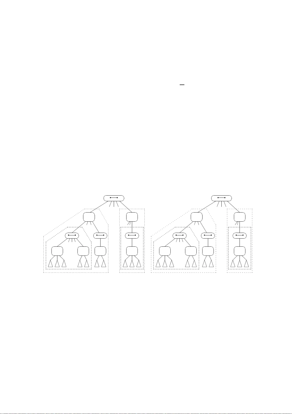
Planar Graph Isomorphis m is in L og-Space ∗ Samir Datta 1 Nutan Limay e 2 Pra jakta Nim bhork ar 2 Thomas Thierauf 3 † F abian W agner 4 ‡ 1 Chennai Mathematical Institute sdatta@cmi. ac.in 2 The Institute of Mathematical Sciences { nutan,praja kta } @imsc.res.in 3 F ak. Elektronik und Info rmatik, HTW Aalen 4 Institut f ¨ ur Theoretisc he Informatik, Univ ersit¨ at Ulm, 89073 Ulm { thomas.thie rauf,fabian.wagner } @uni-ulm.de No v ember 1 1, 2018 Abstract Graph Iso morphism is the prime example of a computational pr oblem with a wide diﬀerence betw een the bes t known low er and upper b ounds on its complexity . W e bridge this gap for a natural and imp ortant special case , pla nar graph isomor phis m, b y presenting an upper b ound that matches the known logspa ce hardness [Lin92]. In fact, w e show the formally stronger res ult that planar gr aph canoniza tio n is in logs pace. This improv es the previously known upper b ound o f A C 1 [MR91]. Our algorithm ﬁrst co nstructs the biconnected co mp one nt tree o f a connected pla- nar gra ph and then reﬁnes ea ch bico nnected comp onent into a trico nnected comp onent tree. The next step is to lo gspace reduce the biconnected plana r g raph isomorphis m and canonization pro blems to those for 3- connected planar gra phs, which ar e known to b e in logspace b y [DLN08]. This is achiev ed by using the ab ov e decompo s ition, and by making signiﬁcant modiﬁca tions to Lindell’s algor ithm for tree canonization, along with changes in the space complexity analysis. The reductio n from the co nnected cas e to the bico nnected case requires further new ideas, including a non-trivia l ca se analysis and a group theor etic lemma to bound the nu mber of automor phisms of a colo red 3-co nnected plana r gr aph. This lemma is cr ucial for the reduction to work in logspace. 1 In tro duction The graph isomorphism problem GI consists of d eciding whether there is a b ijection b etw een the no des of tw o grap h s, which preserve s edges. The w ide gap b et ween the known low er and ∗ A preliminary version of the pap er app eared at † Supp orted by DFG gran t s Scho 302/7 -2 and TO 200/2-2. ‡ Supp orted by DFG gran t s Scho 302/7 -2 and TO 200/2-2. 1 upp er b ound s h as k ept aliv e the researc h interest in GI. The p roblem is clearly in NP , and, by a group theoretic pro of, also in SPP [AK06]. Th is is the cur ren t fron tier of our kno wledge as far as up p er boun ds go. The inabilit y to giv e eﬃcien t algorithms for the problem would lead one to b eliev e that the problem is pro v ably hard. NP -hardness is precluded by a result that states if GI is NP -hard then the p olynomial time hierarc hy collapses to the second lev el [BHZ87 , S c h 88]. What is more surp rising is that not ev en P -hardn ess is kno wn for the pr oblem. The b est we know is that GI is hard for DET [T or04], t he class of problems NC 1 -reducible to the d etermin ant, d eﬁned by Cook [Co o85]. While this enormous gap has motiv ated a stu d y of isomorp hism in g e ner al g raphs, it h as also induced r esearc h in isomorp hism restricted to s p ecial cases of graph s, where this gap can b e reduced. T ournament s are an example of directed graphs w here the DET low er b ound is preserve d [W ag07], while there is a quasi-p olynomial time upp er b oun d [BL83]. T rees are an example of graph s where the lo wer and upp er b ound s matc h and are L [Lin92]. Note that for trees, the p roblem’s c omplexit y crucially dep ends o n the in put enco d ing: if the trees are pr esen ted as strings then th e lo wer and upp er b ound are NC 1 [JT98, Bus97]). Lindell’s log-space result h as b een extended to partial 2-trees, also known as generalized series-parallel graphs [ADK08]. In this pap er we consider planar graph isomorphism and settle its complexit y . Note that trees and partial 2-trees are a sp ecial ca ses of p lanar graphs. Planar Graph Isomorp hism has b een studied in its own righ t since the early days of computer science. W ein b erg [W ei66] present ed an O ( n 2 ) algorithm for testing isomorphism of 3-connected planar graphs. Hop croft and T arjan [HT74] extended this t o general planar graph s , improving th e time complexit y to O ( n log n ). Hop croft and W ong [HW74] fu rther improv ed it to O ( n ). Recen tly K ukluk, Holder, and Co ok [KHC04] ga v e an O ( n 2 ) algorithm for planar graph isomorph ism, w hic h is suitable for p r actical applications. The parallel complexit y of Planar Graph Isomorphism wa s ﬁ rst consid ered by Miller and Reif [MR91] and Ramac handr an and Reif [RR90]. They show ed that the upp er b ound is A C 1 , see also [V er07]. Recen t work has dealt with a fur th er sp ecial case viz. 3-connected planar graph s. Thierauf and W agner [TW08] p resen ted a new upp er b oun d of UL ∩ coUL , making use of the mac hinery dev elop ed for the reac hab ility problem [RA97 ] and sp eciﬁcally for planar reac habilit y [ADR05 , BTV07]. Th ey also show that th e problem is L -hard . F urther p rogress, in the form of a log- space algorithm is made by Datta, L ima ye, and Nim bhork ar [DLN08 ], where the 3-connected planar case is settled, by bu ilding on id eas from [TW08] and u sing Reingold’s construction of unive rsal exp loration sequences [Rei05]. The curr en t wo rk is a n atural culmination of this ser ies where we settle the complexit y question for planar graph isomo rph ism b y p resen ting the ﬁrst log- space algorithm for the problem. In fact, we give a log-space algorithm for th e gr aph c anonization pr oblem , to whic h graph isomorphism reduces. Th e canonizati on inv olv es assig ning to eac h graph an isomor- phism inv arian t, p olynomial length strin g. Our algorithm consists of the follo wing steps. 1. Decomp ose the planar graph into its biconnected comp onen ts and construct a bic on- ne cte d c omp onent tr e e in log-space [ADK08 ] (Section 5). 2. Decomp ose b iconn ected planar comp onent s int o their triconnected comp on ents to ob- tain a tric onne cte d c omp onent tr e e in log-space. This is essen tially a parallel implemen- tation of the sequen tial algorithm of [HT73] (Section 3). 2 3. Inv oke the algorithm of Datta, L im ay e, and Nim bhork ar [DLN08] to canonize the tri- connected comp onen ts of the graph. 4. Canon ize biconnected p lanar graphs by app lying tree canonization ideas from [Lin92] to their triconnected comp onen t trees. Note that, p airwise isomorphism of t w o trees lab elled with the canons of their comp onents d o es not imply isomorphism of the corre- sp ondin g graph s. Lindell’s algorithm and complexit y analysis had to b e mo d iﬁed in a non-trivial wa y for this step to wo rk in log-space (Section 4). 5. Canon ize planar graphs using their biconnected comp onent trees, and for biconnected comp onent s th eir triconnected comp onent trees. F or the canonization again, we use the basic structure of Lin dell’s algorithm. The new ingredients here are, an intrica te case analysis, and a group theoretic lemma (Lemma 5.3) to b oun d th e num b er of automor- phisms of a coloured 3-connected planar graph (Section 5). It also requires a d etailed analysis of th e in terferences of b oth tree structures. Our algorithm works recur s iv ely at v arious places. The ma jor c hallenge w hen dev elopping a recursive log-space algorithm is that very little can b e stored at eac h lev el of the r ecursion. But we must anyw a y b e able to con tinue a computation a t the p oin t w here w e ma de the recursiv e call, when w e r eturn from th e r ecursion. W e solv e these problems by identifying in eac h case app ropriate graph pr op erties that hav e a short description and w hic h can b e used to recompute the p oin t wh ere w e started from. 2 Preliminaries In this section, w e recall some basic graph theoretic notions. A graph G = ( V , E ) is c onne cte d if there is a p ath b etw een an y t w o v ertices in G . F or U ⊆ V let G ( U ) b e the induc e d sub gr aph of G on U . A vertex v ∈ V is an articulation p oint if G ( V \ { v } ) is not connected. A pair of vertic es u, v ∈ V is a sep ar ating p air if G ( V \ { u, v } ) is not connected. A bi c onne cte d gr aph con tains no articulation p oints. A 3-c onne cte d gr aph con tains no separating pairs. A tric onne cte d gr aph is either a 3-connected graph or a cycle or a 3-b ond . A k -b ond is a graph consisting of t wo vertic es joined by k edges. A pair of ve rtices ( a, b ) is said to b e 3 -c onne c te d if there are three or more vertex- disjoint paths b etw een th em. F or a no de v let d ( v ) b e the maximal distance that v has to an y of th e other no des of G . Let C b e the set of no des v of G th at hav e minimal v alue d ( v ). Th e set C is c alled the c enter of G . In other w ord s, v er tices in the cen ter minimize the maximal distance from other v ertices in the graph . Note that if G is a tree s u c h that ev ery path from a lea v e to a lea ve has ev en length, then the center consists of only one no d e, n amely the midp oin t of a longest path in the tree. Let E v b e the set of edges incident to v . A p erm uatation ρ v on E v that h as only one cycle is called a r otation . A r otation scheme for a graph G is a set ρ of r otations, ρ = { ρ v | v ∈ V and ρ v is a rotation on E v } . Let ρ − 1 b e the set of inv erse rotations, ρ − 1 = { ρ − 1 v | v ∈ V } . A rotation sc heme ρ describ es an em b edd in g of graph G in the p lane. If the emb edding is p lanar, we call ρ a planar r otation scheme . Note th at in this case ρ − 1 is a planar rotatio n sc heme as w ell. Allender and 3 Maha j an [AM00] sho we d that a p lanar rotation scheme for a p lanar graph can b e computed in log-space. Tw o g raphs G 1 = ( V 1 , E 1 ) and G 2 = ( V 2 , E 2 ) are said to be iso morphic ( G 1 ∼ = G 2 ) if there is a bijection φ : V 1 → V 2 suc h that ( u, v ) ∈ E 1 if and only if ( φ ( u ) , φ ( v )) ∈ E 2 . Gr aph isomorph ism (GI) is the pr ob lem of deciding whether t wo giv en graph s are isomorph ic. A p lanar graph G , along with its planar emb edding (giv en by ρ ) is called a plane gr aph b G = ( G, ρ ). A p lane graph divides the plane in to regions. E ach s uc h region is called a fac e . Let Planar-GI b e the sp ecial case of GI wh en the giv en graph s are planar. The b iconnected (resp ectiv ely , 3-connected) planar GI is a sp ecial case of Planar-GI when the graphs are biconnected (3-connected) planar graphs. Let G b e a class of graphs. Le t f : G → { 0 , 1 } ∗ b e a function such that f or all G, H ∈ G we ha v e G ∼ = H ⇔ f ( G ) = f ( H ). Then f computes a c omplete invariant for G . If f compu tes for G a graph f ( G ) suc h that G ∼ = f ( G ) then we call f ( G ) the c anon for G . By L we d en ote the languages computable b y a log-space b ounded T ur in g mac h ine. 3 Decomp osition of Biconn ected Planar Gr aphs In this section, w e pr o ve the follo win g theorem. Theorem 3.1 The de c omp osition of bic onne cte d planar gr aphs into tric onne cte d c omp onents is in lo g-sp ac e. Hop croft a nd T arjan [HT73] presente d a sequen tial algorithm fo r th e d ecomp osition of a bico nnected planar graph in to its triconnected co mp onen ts. Their alg orithm recursiv ely remo v es separating pairs from the graph and puts a copy of the separating pair in eac h of the comp onents so formed. The no des in th e separating pair are connected b y a virtual edge. If simp le cycles are split at any intermediate steps then they are com bined later. This giv es a decomp osition whic h is unique [Mac37]. W e d escrib e a log-space algorithm for s uc h a decomp osition of a biconnected planar graph . W e start with deﬁ n itions and then pr o ve some prop erties of separating pairs. Deﬁnition 3.2 In a plane gr aph b G , a sep ar ating p air { a, b } is said to span a face f if b oth its endp oints a, b lie on the b oundary of f . L e t v 0 , v 1 , . . . , v k b e a fac e b oundary. Two sep a- r ating p airs { v i , v j } , { v i ′ , v j ′ } ar e c al le d in tersecting if i < i ′ < j < j ′ , and non-intersect ing otherwise. Lemma 3.3 Every sep ar ating p air sp ans some fac e. T o see th is, n ote that in a plane graph b G , a split comp onent of a separating pair is em b edded in some face. This can b e considered as the sp anned f ace. A separating pair { a, b } that sp ans a face f is called 3- c onne c te d if there are at least thr ee v ertex-disjoin t paths b et ween a, b i.e. there is a path b et we en a, b in b G which is v ertex-disjoin t from the b oundary of f . The follo wing lemma enables us to remov e all the 3-connected separating pairs s im ultaneously . Lemma 3.4 In a plane gr aph b G , 3 -c onne c te d sep ar ating p airs which sp an the same fac e ar e non-interse cting. 4 Pro of. Supp ose { a, c } and { b, d } are tw o 3-connected intersecti ng separating p airs on face f in b G and let P b e a path outside f from b to d . In particular, P does not p ass throu gh a or c . As the p air b, d is 3-connected, it cann ot b e separated f rom the rest of the graph by any other separating pair. Let v b e a vertex that gets separated from b and d when a and c are remo v ed f rom the graph. Since v lies outside f , there is a path outside f fr om a via v to c . Since the grap h is planar, th is path m ust inte rsect P . Thus there is a p ath fr om v to b and d that d o es not pass through a or c . This con tr adicts the assump tion that remo v al of a and c separated v f rom b and d .  Deﬁnition 3.5 Cal l a set of ve rtic es V ′ ⊆ V ( b G ) separable i f ther e exists a 3 -c onne c te d sep- ar ating p air { a, b } in V ( b G ) such that the r emoval of { a, b } divides V ′ into diﬀer ent c onne cte d c omp onents. Otherwise V ′ is c al le d inseparable . Given an insep ar able triple τ = { u, v , w } , deﬁne C τ = { x | { u, v , w , x } is insep ar able } . Note that the no d es of a simp le cycle a re trivial ly inseparable b ecause there are no 3- connected separating pairs. The follo win g lemma states that except for cycles, all biconnected graphs ha v e 3-connected separating p airs and hence the sets C τ deﬁned ab o v e are the 3- connected comp onents of suc h a graph . Lemma 3.6 L et G b e a bic onne cte d planar gr aph. If G is not 3 -c onne cte d and not a c ycle then G has a 3 - c onne cte d sep ar ating p air. Pro of. Let G b e neither 3-connected nor a cycle and let a, b b e a separating pair of G . If a and b are 3-connected then we are done. So assu me that a and b are n ot 3-connected. Let f b e a face spanned by a and b . Then a and b are conn ected by tw o vertex- disjoint paths, sa y P 1 and P 2 , wh ic h form the b oundary of f , and the remo v al of ( a, b ) separates these tw o paths. Since G is not a sin gle cycle, it has more faces apart from f . Therefore f shares some of its edges with another face, sa y f ′ . Consider the common b oundary b et we en f and f ′ . Th e endp oints of this b oun dary , sa y ( u, v ) hav e th ree v ertex-disjoin t paths b et ween them, and hence are 3-connected. Both u and v lie on P 1 or b oth lie on P 2 , since otherwise P 1 and P 2 will not b e sep arated on the remo v al of ( a, b ). Without loss of generalit y , assum e that u, v ∈ P 1 . Let P 1 = { a = v 1 , v 2 , . . . , v k = b } and consider all 3-connected p airs ( v i , v j ) of v ertices th at lie on P 1 . Pic k a pair, sa y ( v i , v j ), that is maximally apart on P 1 . W e claim that ( v i , v j ) is a sep arating pair: if not, th er e exists a path outside f from v i ′ to v j for some i ′ < i , or from v j ′ to v i for some j ′ > j . In the ﬁr st case, ( v i ′ , v j ) is a 3-connected pair that is f urther apart than ( v i , v j ), in the second case the same holds for ( v i , v j ′ ). But this con tradicts the c h oice of ( v i , v j ).  Hence, with inseparable triples w e can compute triconnected comp onen ts. If a trip le of v ertices is inseparable, then it is part of the same triconnected comp onent . F or distinct τ 1 , τ 2 , the sets C τ 1 and C τ 2 are either disjoint or iden tical. This allo ws us to id entify any suc h C τ with the lexicographical smallest τ 0 (considering the lab els of v ertices in τ lexicographically sorted) such that C τ = C τ 0 . This is the approac h of Algorithm 1 b elo w. First, the algorithm computes all 3-connected separating pairs in the set S . F r om these, w e get all the 3-b onds. Th e for -lo op f rom line 8 on computes the 3-connected comp onen ts C τ : I n line 9, we searc h fo r the ﬁrst insep arable triple τ / ∈ { C τ h | 1 ≤ h < i } that can b e separated from all previous ones. In lines 11 and 12, we searc h for all τ j ⊆ C τ i . By Lemma 3.6, 5 Algorithm 1 Algorithm to decomp ose a graph int o triconnected comp onents. Input: Biconnecte d planar graph G = ( V , E ). Output: The tr iconnected comp onen ts of G . 1: ﬁx a planar embed ding b G of G . 2: for all faces f of b G do 3: S f ← { ( u, v ) | ( u, v ) is a 3-connected separating pair that span s f } 4: S ← ∪ f ∈ b G S f the set of 3-connected separating pairs 5: for all ( u, v ) ∈ S do 6: if ( u, v ) ∈ E then ou tp ut a 3-b ond for ( u, v ) 7: compute the set of all insep arable tr ip les τ 1 , . . . , τ k 8: for i ← 1 to k do { compute 3-connected component s } 9: if ∀ h < i τ i ∪ τ h is a separable set then 10: C i ← τ i { create new 3-connecte d comp onen t using inseparable triple τ i } 11: for j ← i + 1 to k do 12: if τ i ∪ τ j is an ins ep arable set then C i ← C i ∪ τ j 13: output the indu ced sub graph on C i without edges corresp ondin g to 3-b onds, including virtual edges { s ∈ S | s ⊆ C i } it suﬃces to consider the pairs in S t o c hec k whether a set is separable or not. The s et C i ﬁnally equals C τ i . In line 13 w e compu te the triconnected comp onen t induced b y C τ i . An example of a d ecomp osition is p ro vided in Figure 1. Eac h step in the algorithm can b e imp lemented in log-space. F or instance, a combina- torial em b edding for planar graph s can b e computed in log-space [AM00 ]. Separating pairs, inseparable triples and the tr iconn ected comp onen ts can b e computed in log-space, making oracle queries to u ndirected reac habilit y [Rei05]. f b e c d d b a a c G 1 b f a d G 2 G 4 b c d a e c d G 4 G 2 G 3 b G G 1 T G 3 c Figure 1: The decomp osition of a biconnected planar graph b G . Its triconnected comp onen ts are G 1 , . . . , G 4 and th e corresp ond ing triconnected comp onen t tree is T . In b G , the pairs ( a, b ) and ( c, d ) are 3 -connected separating pairs. The inseparable triples a re { a, b, c } , { b, c, d } , { a, c, d } , { a, b, d } , { a, b, f } , and { c, d, e } . He nce th e triconnected comp onents are the induced graphs G 1 on { a, b, f } , G 2 on { a, b, c, d } , and G 4 on { c, d, e } . Since the 3-connected separating pair ( c, d ) is connected by an edge in b G , we also get { c, d } as triple-b ond G 3 . The virtual edges corresp ond ing to the 3-connected s eparating pairs are dra wn with dashed lines. 6 The triconnected comp onen t t ree. Construct a graph T suc h that its no des corresp ond to triconnected comp onen ts a nd separating pairs, see Figure 1 . T here is an edge b et wee n a tric onne cte d c omp onent no de and a sep ar ating p air no de if the vertice s of the separating pair a re con tained in t he trico nnected comp onent. Tw o triconnected co mp on ent n o des or separating pair no des do not sh are an edge. It is ea sy to see t hat T is a tree, referred to as the tric onne cte d c omp onent tr e e of G . Con v ersely , giv en T , w e deﬁn e graph ( T ) = G , th e graph whic h h as the triconnected comp onen t tree T . W e list some prop er ties of T . Lemma 3.7 The gr aph T deﬁne d ab ove has the fol lowing pr op erties: 1. T is a tr e e and al l the le aves of T ar e tric onne cte d c omp onents. 2. Each p ath i n T i s an alternating p ath of sep ar ating p airs and tric onne cte d c omp onents. Henc e, a p ath b etwe en two le aves always c ontains an o dd numb er of no des and ther efor e T has a unique c enter no de. 3. With an arbitr ary sep ar ating p air no de as r o ot, T has o dd depth. 4. A 3 -b ond is intr o duc e d as a child of a se p ar ating p air only as an indic ator that the vertic es of the sep ar ating p air have an e dge b etwe en them i n G . Henc e a 3 -b ond is always a le af no de. In [HT73] it is a k -b ond, wher e k is the numb er of c omp onents forme d by the r emoval of the sep ar ating p air. Observe, k is the numb er of childr en of its p ar ent sep ar ating p air and c an b e c ompute d e asily. Pro of. W e only sho w the ﬁrs t claim. Sup p ose T h as a cycle C . By deﬁnition, C is an alter- nating cycle of separating pairs and triconnected comp onents, C = ( p 1 , c 1 , p 2 , c 2 . . . , p r , c r , p 1 ). Remo ve an y separating pair p i from C . T hen the triconnected comp onents c i − 1 and c i re- main conn ected through the other elements of th e cycle, con tr ad icting the assumption that p i separates them.  4 Canonization of Biconnected Planar Graphs In this section, we giv e a log-space algorithm to canonize biconnected planar graphs. F or this, w e deﬁn e an isomorph ism ordering on triconnected comp onent trees w hic h is similar to that of Lin dell’s tree isomorp hism ord er in g. W e ﬁrst give a brief o verview of Lindell’s algorithm and then d escrib e our canonizatio n pro cedur e. 4.1 Ov er view of Lindell’s A lgorithm Lindell [Lin92] ga v e a log-space algo rithm for tree canonization. The algorithm is based on an order relation ≤ on trees deﬁned b elo w. The order relation has th e prop erty that t w o trees S and T are isomorphic if and only if S = T . Because of this pr op ert y it is called a c anonic al or der . C learly , an algorithm that decides the order can b e used as an isomorphism test. Lindell sh o wed ho w to extend suc h an algorithm to compute a canon for a tree in log-space. Let S and T b e t w o trees with ro ot s and t , resp ectiv ely . The canonical order is deﬁned as follo ws. S < T if 1. | S | < | T | , or 7 2. | S | = | T | but # s < # t , where # s and # t are the n umber of c hildren of s and t , resp ectiv ely , or 3. | S | = | T | and # s = # t = k , bu t ( S 1 , . . . , S k ) < ( T 1 , . . . , T k ) lexicographically , where it is indu ctiv ely assu med that S 1 ≤ . . . ≤ S k and T 1 ≤ . . . ≤ T k are the ordered s u btrees of S and T r o oted at the k c hildren of s and t , resp ectiv ely . The comparisons in steps 1 and 2 can b e made in log-space. Lindell pro ve d that even the third s tep can b e p erformed in log-space u sing two-pr onge d depth-ﬁrst searc h , and cr oss- c omp aring only a c h ild of S with a c hild of T . This is b rieﬂy describ ed b elo w: • Find the n umber of min im al sized children of s and t . If these num b ers are diﬀerent then the t ree with a larger num b er of minimal children is d eclared to b e smaller. If equalit y is fo und then remem b er the minimal size and c hec k for the next size . This pro cess is co nti nued till an inequalit y in the sizes is detec ted or all the c hildren o f s and t are exhausted. • If s and t ha ve the same num b er of c hildren of eac h size then assume that the children of s and t are partitioned into size- classes (referred to as blo c k s in [Lin92]) in the increasing order of the the sizes of the su btrees r o oted at them. That is, the k c h ild ren of s and t are partitioned into groups, such that th e i -th group is of cardinalit y k i and the subtr ees in the i -th group all h a ve size N i , where N 1 < N 2 < · · · . It follo ws th at P i k i = k and P i k i N i = n − 1. Th en compare the c hildren in eac h size-cla ss recursiv ely as follo ws: Case 1, k = 0 . Hence s and t ha v e n o c hildren. T hey are isomorp h ic as all one-no d e trees are isomorp h ic. W e conclud e that S = T . Case 2, k = 1 . Recursivel y consider the grand -c h ildren of s and t . No space is needed for the r ecur siv e call. Case 3, k ≥ 2 . F or eac h of the subtrees S j compute its order proﬁle. The order proﬁle consists of three coun ters, c < , c > and c = . These counte rs indicate the num b er of subtrees in the size-cla ss of S j that are r esp ectiv ely smaller than, greater than, or equal to S j . The counters are computed by m aking cross-comparisons. Note, that isomorphic sub trees in the same size-class hav e the same order proﬁ le. There- fore, it suﬃces to chec k th at eac h such order proﬁle o ccurs the same num b er of times in eac h size-class in S and T . T o p erform this c hec k, compare the diﬀerent ord er pr oﬁles of ev ery size class in lexicog raphic order. The sub trees in the size-cla ss i of S and T , whic h is currently b eing consid ered, with a count c < = 0 form the ﬁ rst isomorphism class. The size o f this isomorphism cla ss is compared ac ross the trees b y comparing the v alues o f the c = v ariables. If these v alues matc h then b oth trees ha v e the s ame n umber of minimal c hildren. Note that the lexicographical next larger ord er p r oﬁle has the curr en t v alue of c < + c = as its v alue for the c < -coun ter. This wa y , one can lo op through all the order proﬁles. If a diﬀerence in the ord er proﬁles of th e sub tr ees of S and T is found th en the lexicographical smaller order proﬁle deﬁn es the smaller tree. 8 The last order proﬁle considered is the one with c < + c = = k for the current counters. If this p oin t is passed without u nco vering an inequalit y then the trees m ust b e isomorph ic and it follo ws that S = T . Since P i k i N i ≤ n , the follo win g recur s ion equation for the space complexit y holds. F or eac h new size class, the work-tape allo cated for th e former computations can b e reused . S ( n ) = max i {S ( N i ) + O (log k i ) } ≤ max i { S  n k i  + O (log k i ) } , where k i ≥ 2 for all i . It is not hard to see that S ( n ) = O (log n ). 4.2 Isomorphism Order of T riconnected Comp onen t T rees W e no w d escrib e an isomorphism ord er p ro cedure for t w o tr iconn ected c omp onent trees S and T , corresp ondin g to tw o biconnected planar graphs G and H , resp ectiv ely . Both, S and T are ro oted at sep arating pair no des, as d escrib ed in Section 3, sa y s = ( a, b ) and t = ( a ′ , b ′ ). Therefore w e also write S ( a,b ) and T ( a ′ ,b ′ ) . Th ey ha v e separating pair no des at o d d lev els and triconnected comp onent no des at ev en leve ls. Figure 2 sh ows tw o trees to b e compared. Our canonical order p ro cedure is m ore complex than Lindell’s algorithm, b ecause eac h no d e of the tree is a separating pair or a triconnected comp on ent. T hus in particular, unlik e in the case of L in dell’s algorithm, t w o lea ves in a triconnected comp onen t tree are n ot alw ays isomorphic. In th e easiest case the comp onents to these lea v es are not of the same size. W e start by deﬁn ing the size of a triconnected comp onent tree. b a s G 1 . . . . . . . . . . . . G k s 1 . . . . . . . . . . . . . . . . . . t a ′ b ′ H k H 1 t 1 s l k t l k s l 1 t l 1 S ( a,b ) T ( a ′ ,b ′ ) S 1 S l k T 1 T l k S G 1 S G k T H k T H 1 Figure 2: T riconnected comp onent trees. Deﬁnition 4.1 F or a tric onne cte d c omp onent tr e e T , the size of an ind ividual comp on ent no de C of T is the numb er n C of no des in C . Note that the sep ar ating p air no des ar e c ounte d in in every c omp onent wher e they o c c u r. The size of the tree T , denote d by | T | , is the sum of the sizes of its c omp onent no des. Note that the size of T is at least as large as the num b er of vertice s in graph ( T ), the graph corresp ondin g to the triconnected comp onent tree T . 9 W e d eﬁne the isomorph ism order < T for S ( a,b ) and T ( a ′ ,b ′ ) b y ﬁr st comparing their sizes, then the num b er of c hildren of s and t . Th ese tw o steps are exactly the same as in Lindell’s algorithm. If equalit y is found in these t w o steps, then in the thir d step we mak e recurs ive comparisons of the subtrees of S ( a,b ) and T ( a ′ ,b ′ ) . How ev er, her e it do es not suﬃce to compare the ord er p roﬁles of the sub tr ees in the diﬀerent size classes as in Lind ell’s algorithm exp lained ab o v e. W e need a f urther comparison s tep to ensu re that G and H are indeed isomorph ic. T o see th is assu m e that s and t ha v e t wo c h ildren eac h, G 1 , G 2 and H 1 , H 2 suc h that G 1 ∼ = H 1 and G 2 ∼ = H 2 . Still we cannot conclude that G and H are isomorphic b ecause it is p ossible that the isomorphism betw een G 1 and H 1 maps a to a ′ and b to b ′ , but t he isomorphism b et we en G 2 and H 2 maps a to b ′ and b to a ′ . Then these t w o isomorphisms cannot b e extended to an isomorphism b etw een G and H . F or an example see Figure 3 on page 12. T o h an d le this, we in tro duce the notion of an orientation of a sep ar ating p air . A separating pair gets an orien tation from sub trees ro oted at its c hildren. Also, ev ery subtree r o oted at a triconnected co mp onen t no de g iv es an orien tation to the paren t separating pair. If the orien tation is consisten t, then w e deﬁne S ( a,b ) = T T ( a ′ ,b ′ ) and we will sho w that G and H are isomorphic in this case. Isomorphism order of tw o subtrees ro oted at triconnected comp onents. W e con- sider the isomorphism order of t w o s u btrees S G i and T H j ro oted at triconnected comp onen t no des G i and H j , resp ectiv ely . W e d istinguish the follo wing cases. Case 1, G i and H j ar e of diﬀer ent typ es . G i and H j can be ei ther 3-b onds o r cycl es or 3-connected comp onen ts. If the t yp es of G i and H j are diﬀerent, we immediately detect an inequalit y , as it suﬃces to c hec k whether eac h of them is a cycle or a 3-b ond or neither of them. W e deﬁne a canonical ord er among subtrees ro oted at triconnected comp onen ts in this ascending order: 3-b on d , cycle, 3-connected comp onent, su c h that e.g. S G i < T T H j if G i is a 3-b ond and H j is a cycle. Case 2, G i and H j ar e 3 -b onds . In this case, S G i and T H j are lea v es, immediately deﬁne S G i = T T H j . Clearly , G i ∼ = H j as all 3-b ond s are isomorphic. Case 3, G i and H j ar e cycles or 3 -c onne cte d c omp onents . W e construct the canons of G i and H j and compare th em b it-b y -b it. T o canonize a cycle, w e trav erse it starting fr om the virtual ed ge that corresp ond s to its paren t, and then tra versing the en tire cycle along the edges enco untered. There are t w o p ossible trav ersals dep end ing on w h ic h direction of the starting edge is c hosen. Th us, a cycle has t w o p ossible canons. T o canonize a 3-connected comp onent G i , we us e the log-space algorithm fr om Datta, L i- ma ye, and Nimbhork ar [DLN08]. Besides G i , the algorithm gets as inp ut a starting edge and a com b inatorial em b eddin g ρ of G i . W e alw ays tak e the virtual edge ( a, b ) corresp onding to G i ’s paren t as the starting edge. Then there are t w o choic es for the d irection of this ed ge, ( a, b ) or ( b, a ). F urther, a 3-connected graph has t wo planar com binatorial emb eddings [Whi33]. Hence, there are four p ossible wa ys to canonize G i . W e start the canonization of G i and H j in all the p ossible wa ys (t wo if they are cycles and f our if they are 3-connected comp onen ts), and compare these canons bit-b y-bit. L et C g and C h b e t w o canons to b e compared. The base case is that G i and H j are leaf no des and therefore con tain no further virtual edges. In this case we use the lexicographic order b et we en C g and C h . If G i and H j con tain fur th er virtual edges then these edges are sp eciall y treated in the bit wise comparison of C g and C h : 10 1. If a virtual edge is trav ersed in th e constru ction of one of th e canons C g or C h but not in the other, then we d eﬁ ne the one without th e v ir tual edge to b e the smal ler c anon. 2. If C g and C h encoun ter v ir tual edges ( u, v ) and ( u ′ , v ′ ) corresp onding to a child of G i and H j , resp ectiv ely , we need to recursively compare the subtr ees ro oted at ( u, v ) and ( u ′ , v ′ ). If we ﬁnd in the recursion that one of the subtr ees is s m aller than the other, then the canon with the smaller subtree is deﬁn ed to b e the smal ler c anon. 3. If we ﬁ n d that the subtr ees ro oted at ( u, v ) and ( u ′ , v ′ ) are equ al then we lo ok at the orien tations giv en to ( u, v ) and ( u ′ , v ′ ) by their c h ildren. T his orien tation, called the r efer enc e orientation , is d eﬁ ned b elo w. If one of the canons tra ve rses the virtual edge in the direction of its reference orien tation b u t the other one not, then the one with the same direction is deﬁned to b e the smal ler c anon. W e eliminate the canons wh ic h were foun d to b e the larger canons in at least one of th e comparisons. In the end, the canons th at are not eliminated are the minimum c anons . If w e ha v e minimum canons for b oth G i and H j then w e deﬁne S G i = T T H j . The construction of the canons also deﬁnes an isomorph ism b et ween the su bgraphs describ ed by S G i and T H j , i.e. graph ( S G i ) ∼ = graph ( T H j ). F or a single triconnected comp on ent this f ollo ws from Datta, Lima ye, and Nimbhork ar [DLN08]. If the trees con tain sev eral comp onen ts, then our deﬁnition of S G i = T T H j guaran tees that we can com bin e the isomorph isms of the comp onen ts to an isomorphism b et ween graph ( S G i ) and graph ( T H j ). Finally , we deﬁn e th e orientation given to the p ar ent sep ar ating p air of G i and H j as the direction in whic h th e minimum canon tra verses this edge. If the minim um canons are obtained for b oth c hoices of directions of the edge, we sa y that S G i and T H j are symmetric ab out their p ar ent sep ar ating p air , an d th us do not gi v e an orien tation. Th is ﬁnish es th e description of the order for th e case of sub trees ro oted at triconnected comp onents. Observe , that we d o not need to compare the sizes and the degree of the ro ot n o des of S G i and T H j in an inte rmediate step, as it is done in Lind ell’s algorithm for subtrees. That is, b ecause th e d egree of the ro ot no d e G i is enco d ed as the num b er of virtual edges in G i . The size of S G i is c h ec ked by th e length of the minimal canons for G i and w hen we compare the sizes of th e children of the ro ot no de G i with those of H j . Isomorphism order of t wo subtrees ro oted at separating pairs. The ﬁrst three steps of the isomorph ism ord ering are p erform ed similar to that of [Lin92] maintaining the ord er proﬁles. No w w e a ssume that the subtrees a re partitioned i nto isomorphism classes. The additional step in v olv es comparison of orientations giv en by the corresp ond ing isomorph ism classes deﬁned as f ollo ws: Let ( G 1 , . . . , G k ) b e t he c hildren of the r o ot ( a, b ) of S ( a,b ) , and ( S G 1 , . . . , S G k ) be the subtrees ro oted at ( G 1 , . . . , G k ). Similarly let ( H 1 , . . . , H k ) b e the c hildren of the ro ot ( a ′ , b ′ ) of T ( a ′ ,b ′ ) and ( T H 1 , . . . , T H k ) b e the subtrees ro oted at ( H 1 , . . . , H k ). W e ﬁ rst order the subtrees, sa y S G 1 ≤ T · · · ≤ T S G k and T H 1 ≤ T · · · ≤ T T H k , and v erify that S G i = T T H i for all i . If we ﬁnd an in equalit y then the one w ith the smallest ind ex i deﬁn es the order b et w een S ( a,b ) and T ( a ′ ,b ′ ) . Now assume that S G i = T T H i for all i . Ind uctiv ely , the corresp onding split comp onent s are isomorp h ic, i.e. graph ( S G i ) ∼ = graph ( T H i ) for all i . The next comparison concerns the orientat ion of ( a, b ) and ( a ′ , b ′ ). W e already explained ab o v e th e orienta tion giv en b y eac h of the S G i ’s to ( a, b ). W e deﬁn e a r efer enc e orientation 11 for the ro ot no des ( a, b ) and ( a ′ , b ′ ) which is giv en by th eir c hildren . This is done as follo ws. W e partition ( S G 1 , . . . , S G k ) into classes of isomorph ic subtr ees, say I 1 < T . . . < T I p for some p ≤ k , and s imilar ( T H 1 , . . . , T H k ) into I ′ 1 < T . . . < T I ′ p . It follo ws that I j and I ′ j con tain the same num b er of su btrees for ev ery j . • C on s ider the orien tation give n to ( a, b ) b y an isomorphism class I j : F or eac h isomor- phism class I j w e compute an orientation c ounter , whic h is a pair O j = ( c → j , c ← j ), where c → j is the num b er of s u btrees of I j whic h giv e one orient ation, sa y ( a, b ), and c ← j is the n umber of subtrees from I j whic h giv e the other orien tation, ( b, a ). The larger n umber decides the orien tation giv en to ( a, b ). If these num b ers are equal, or if eac h comp onent in this class is symmetric ab out ( a, b ) then no orien tation is giv en to ( a, b ) b y this class, and the class is said to b e symmetric ab out ( a, b ). Note that in an isomorphism class, either all or none of the comp onen ts are sy m metric ab out the parent. • T h e r efer enc e orienta tion of ( a, b ) is d eﬁned as the orien tation giv en to ( a, b ) by th e smallest non-symmetric isomorph ism class. If all i somorphism cla sses are symmetric ab out ( a, b ), then we say that ( a, b ) h as no r efer enc e orientation . W e order all the orien tation counte rs O j = ( c → j , c ← j ) s uc h that the ﬁ rst comp onent c → j is the counter f or the reference orien tation of ( a, b ). Let O ′ j = ( d → j , d ← j ) b e the corresp onding orient ation counte rs for th e isomorph ism classes I ′ j . No w w e compare the orien tation coun ters O j and O ′ j for j = 1 , . . . , p . If they are all p airwise equ al, th en the graph s G and H are isomorphic and we d eﬁne S ( a,b ) = T T ( a ′ ,b ′ ) . Otherwise, let j b e the smallest in dex suc h that O j 6 = O ′ j . Then we d eﬁne S ( a,b ) < T T ( a ′ ,b ′ ) if O j is lexicographically smaller than O ′ j , and T ( a ′ ,b ′ ) < T S ( a,b ) otherwise. This ﬁnish es the deﬁnition of th e order. F or an example, see Figure 3. b ′ a b G b ′ a ′ H a b b b ′ a ′ a ′ a b ′ b ′ a b a ′ a ′ a G 1 G 2 H 1 H 2 b H 0 G 0 S ( a,b ) T ( a ′ ,b ′ ) Figure 3: The graphs G and H h a ve the s ame triconnected comp onen t trees but are not isomorph ic. In S ( a,b ) , the 3 -b ond s form o ne iso morphism cla ss I 1 and the other t w o comp onent s form the second isomorp hism class I 2 , as they all are p airwise isomorp hic. The non-isomorphism is detected by comparing the directions give n to the paren t separating pair. W e hav e p = 2 isomorphism classes and for the orienta tion counters w e ha ve O 1 = O ′ 1 = (0 , 0) , whereas O 2 = (2 , 0) and O ′ 2 = (1 , 1) and hence O ′ 2 is lexicographically smaller than O 2 . Therefore we hav e T ( a ′ ,b ′ ) < T S ( a,b ) . 12 Summary of the steps in the isomorphism order. Th e isomorphism order of t wo triconnected comp onent trees S and T ro oted at separating pairs s = ( a, b ) and t = ( a ′ , b ′ ) is deﬁned S ( a,b ) < T T ( a ′ ,b ′ ) if: 1. | S ( a,b ) | < | T ( a ′ ,b ′ ) | or 2. | S ( a,b ) | = | T ( a ′ ,b ′ ) | bu t # s < # t or 3. | S ( a,b ) | = | T ( a ′ ,b ′ ) | , # s = # t = k , but ( S G 1 , . . . , S G k ) < T ( T H 1 , . . . , T H k ) lexicograph- ically , w here w e assume that S G 1 ≤ T . . . ≤ T S G k and T H 1 ≤ T . . . ≤ T T H k are the ordered subtrees of S ( a,b ) and T ( a ′ ,b ′ ) , resp ectiv ely . T o compute th e order b et ween th e subtrees S G i and T H i w e compare lexicographically the canons of G i and H i and r e cur- sively the subtrees ro oted at the children of G i and H i . Note, that these c hildr en are again separating p air no des. 4. | S ( a,b ) | = | T ( a ′ ,b ′ ) | , # s = # t = k , ( S G 1 ≤ T . . . ≤ T S G k ) = T ( T H 1 ≤ T . . . ≤ T T H k ), but ( O 1 , . . . , O p ) < ( O ′ 1 , . . . , O ′ p ) lexicographically , w here O j and O ′ j are the orien tation coun ters of the j th isomorphism classes I j and I ′ j of all the S G i ’s and the T H i ’s. W e sa y that t w o triconnected comp onent tr ees S e and T e ′ are e qual ac c or ding to the isomor- phism or der , denoted by S e = T T e ′ , if neither S e < T T e ′ nor T e ′ < T S e holds. The f ollo wing theorem states that t wo trees are = T -equal, precisely when the und erlying graphs are isomor- phic. Theorem 4.2 The bic onne cte d planar gr aphs G and H ar e isomorphic if and only if ther e is a choic e of sep ar ating p airs e, e ′ in G and H such that S e = T T e ′ when r o ote d at e and e ′ , r esp e ctively. Pro of. Assume that S e = T T e ′ . The argument is an induction on the d epth of the trees that follo ws the inductive d eﬁnition of the isomorphism ord er. Th e induction go es fr om depth d to d + 2. If the grandc hildren of separating p airs, sa y s and t , are = T -equal up to step 4, then w e compare the children of s and t . If they are equal th en w e can extend the = T -equalit y to the separating p airs s and t . When sub trees are rooted at separating pair nodes, the comparison describ es an o rder on the su btrees whic h corresp ond to split comp onen ts of the separating pairs. The order describ es an isomorp hism among the s plit comp onent s. When subtrees are rooted at triconnected comp onen t no des, sa y G i and H j , the c om- parison states equalit y if the comp onen ts ha v e the same canon, i.e. are isomorphic. By the induction h yp othesis w e kno w that the c hildr en rooted at virtual edges of G i and H j are isomorphic. The equ alit y in the comparisons indu ctiv ely describ es an isomorphism b et we en the ve rtices in the c hildren of the r o ot no des. Hence, the isomorph ism b et ween the children at an y leve l can b e extended to an isomor- phism b etw een th e corresp on d ing su bgraphs in G and H and therefore to G and H itself. The rev erse direction holds obviously as well . Namely , if G a nd H are isomorp hic and there is an isomorph ism that maps the separating pair ( a, b ) of G to the separating pair ( a ′ , b ′ ) of H , then the tr iconn ected comp onent trees S ( a,b ) of G and T ( a ′ ,b ′ ) of H rooted resp ectiv ely at ( a, b ) and ( a ′ , b ′ ) will clearly b e equal. Hence, such an isomorphism mapps separating pairs o f G on to separating pairs o f H . This isomorphism d escrib es a p erm utation o n the 13 split comp onents of separat ing p airs, whic h means w e hav e a p erm utation on triconnected comp onent s, the c hildren of the s eparating pairs. By ind u ction hyp othesis, the children (at depth d + 2) of tw o su c h triconnected comp onents are isomorp hic and equal according to = T . More formally , one can argue ind uctiv ely on the depth of S ( a,b ) and T ( a ′ ,b ′ ) .  4.3 Complexit y of t he Isomorphism Order A lgorithm W e analyse the space complexit y of the isomorphism o rder algorithm. Th e ﬁrst tw o st eps of the isomorphism ord er algorithm can b e computed in log-space as in Lindell’s algo- rithm [Lin92]. W e sh ow that steps 3 and 4 can also b e p erform ed in log-space. W e u se the algorithm of Datta , Lima y e, and Nim bhork ar [DLN08] to canonize a triconnected com- p onent G i of size n G i in space O (log n G i ). Comparing t w o subtrees ro oted at triconnected comp onen ts. F or this, we consid er t wo subtrees S G i and T H j with | S G i | = | T H j | = N ro oted at triconnected comp onen t n o des G i and H j , resp ectiv ely . The cases that G i and H j are of diﬀerent t yp es or are b oth 3-b onds are easy to handle. Assume now that b oth are cycle s or 3-connected comp onents. Th en w e start constructing and comparing a ll the p ossible ca nons of G i and H j . W e eliminate the larger ones and mak e r ecursiv e comparisons when ever the canons en counter virtual edges sim ultaneously . W e can ke ep tr ack of the canons, wh ic h are not eliminated, in constant sp ace. Supp ose we constru ct and compare t w o canons C g and C h and consider the moment wh en w e encounte r vir tual edges ( a, b ) and ( a ′ , b ′ ) in C g and C h , resp ectiv ely . No w we recursively compare the subtrees r o oted at the separating p air n o des ( a, b ) a nd ( a ′ , b ′ ). Note, t hat w e cannot aﬀord to store the entire work-tape con tent. It suﬃces to store the inform ation of • the canons which are n ot eliminated, • w h ic h canons encountered the virtual edges corresp ondin g to ( a, b ) and ( a ′ , b ′ ), and • the direction in whic h the v ir tual edges ( a, b ) and ( a ′ , b ′ ) were encount ered. This tak es altogether O (1) space. When a recur siv e call is completed, w e look at the wo rk-tap e and compute th e canons C G and C h . T h erefore, recompute the p aren t separating pair of the comp onen t, w h ere the virtual edge ( a, b ) is con tained. With a lo ok on the bits stored on the w ork-tap e, w e can recompute the canons C g and C h . Recompute for them, where ( a, b ) and ( a ′ , b ′ ) are encountered in the correct dir ection of the edges and r esume the compu tation from that p oin t. Although w e only n eed O (1) space p er recurs ion lev el, we cannot guarante e y et, that the implemen tation of th e algorithm describ ed so far w orks in log-space. The pr ob lem is, that the subtrees where we go int o recursion might b e of size > N / 2 and in this case the recursion depth can get to o large. T o get around this problem, we chec k whether G i and H j ha v e a large c hild, b efore starting the construction and comparison of th eir canons. A lar ge child is a child which h as size > N / 2. If w e ﬁnd a large c hild of G i and H j then w e compare them a priori and store the result of their recur siv e comparison. Because G i and H j can ha v e at most one large c h ild eac h , this needs only O (1) additional bits. No w , whenev er the v ir tual edges corresp ond ing to the large children from S G i and T H j are en countered sim ultaneously in a canon of G i and H j , the stored resu lt can b e u s ed, th us a vo iding a recur s iv e call. 14 Comparing tw o subtrees ro oted at separating pairs. Consid er tw o su b trees S ( a,b ) and T ( a ′ ,b ′ ) of s ize N , ro oted at separating pair no des ( a, b ) and ( a ′ , b ′ ), resp ectiv ely . W e start comparing all the subtrees S G i and T H j of S ( a,b ) and T ( a ′ ,b ′ ) , resp ectiv ely . These subtrees are r o oted at triconnected comp onents and we can us e the imp lemen tation describ ed ab o ve. Therefore, we store on the work-ta p e the counters c < , c = , c > . If they tur n out to b e pairwise equal, we compute the orient ation count ers O j and O ′ j of the isomorphism classes I j and I ′ j , for all j . Th e isomorp hism classes are computed via th e order proﬁles of the s u btrees, as in Lindell’s algorithm. When we return from recursion, it is an easy task to ﬁnd ( a, b ) and ( a ′ , b ′ ) again, since a triconnected comp on ent has a un ique paren t, whic h alwa ys is a separating pair no d e. Sin ce w e h a ve the coun ters c < , c = , c > and the orien tation counters on the work-tape, w e can pro ceed with the n ext comparison . Let k j b e the num b er of s ubtrees in I j . T he coun ters c < , c = , c > and the orien tation coun ters need altogether at most O (log k j ) s pace. F rom the orien tation coun ters w e also get the reference orien tation of ( a, b ). Let N j b e the size of the subtrees in I j . Then we h a ve N j ≤ N /k j . T his would lead to a log-space implemen tation as in L in dell’s algorithm except for the case th at N j is large, i.e. N j > N / 2. W e h andle the case of large c hildren as ab o v e: we recurse on large c hildren a p riori and store th e result in O (1) b its. Then we pro cess the other subtrees of S ( a,b ) and T ( a ′ ,b ′ ) . When w e reac h the size-class of th e large c hild, w e know the r eference orien tation, if an y . No w w e use the stored result to compare th e orienta tions giv en by the large c hildren to their resp ectiv e paren t, and return the result accordingly . As seen ab ov e, while comparing tw o trees of size N , the algorithm uses no space for making a r ecursiv e call for a su btree of size larger than N/ 2, and it uses O (log k j ) space if the su btrees are of size at most N /k j , where k j ≥ 2. Hence w e get the same r ecurrence for the space S ( N ) as Lindell: S ( N ) ≤ max j S  N k j  + O (log k j ) , where k j ≥ 2 for all j . T h us S ( N ) = O (log N ). Note that the n um b er n of no d es of G is in general s maller than N , b ecause the separating pair no des o ccur in all comp onen ts split oﬀ by this pair. Bu t we certainly ha v e n < N ≤ O ( n 2 ) [HT73]. This pro v es the follo wing theorem. Theorem 4.3 The isomorp hism or der b etwe en two tric onne cte d c omp onent tr e es of bic on- ne cte d planar gr aphs c an b e c ompute d in lo g-sp ac e. 4.4 The Canon of a B iconnected Planar Graph Once we kno w the ordering among the sub trees, it is straight forwa rd to output the canon of the triconnected comp onent tree T . W e trav erse T in the tree isomorphism order as in Lindell [Lin92], outputting the canon of eac h of the no d es along with virtual edges and delimiters. That is, we ou tp ut a ‘[’ w hile going do wn a subtree, and ‘]’ while going u p a subtr ee. W e need to choose a sep arating pair as ro ot for the tree. S ince th er e is no distinguished separating pair, we simply cycle through all of them. Since there are less than n 2 man y separating p airs, a log-space tr ansducer can cycle thr ough all of them and can determine the 15 separating pair which, when chosen as th e r o ot, leads to the lexicographically minimum canon of S . W e describ e th e canonization pro cedur e for a ﬁxed ro ot, s ay ( a, b ). The canonization pr o cedure h as tw o steps. In the ﬁ rst step w e compute wh at w e call a c anonic al list for S ( a,b ) . This is a list of the edges of G , also including virtu al edges. In the second step we compute the ﬁn al canon from the canonical list. Canonical list of a subtree ro oted a t a separa t ing pair. Consider a subtree S ( a,b ) ro oted at the sep arating pair no de ( a, b ). W e start with computing the reference orien tation of ( a, b ) an d outpu t th e edge in this d irection. This can b e done b y comparing the c hildren of the separating p air no de ( a, b ) according to their isomorp hism ord er with the help of the oracle. Then we recursive ly outpu t the canonical lists of th e sub trees of ( a, b ) according to the increasing isomorphism order. Among isomorph ic siblings, those which giv e the reference orien tation to the p aren t are consid ered b efore those wh ic h giv e the rev erse orien tation. W e denote this canonical list of edges l ( S, a, b ). If the su btree ro oted at ( a, b ) do es not giv e any orien tation to ( a, b ), th en tak e that orientati on for ( a, b ), in whic h it is encoun tered dur ing the construction of the ab ov e canon of its p arent. Assume n ow, the paren t of S ( a,b ) is a tric onnected co mp on ent. In the symmetric case , S ( a,b ) do es not giv e an orien tation ( a, b ) to its p aren t. T hen tak e the reference orientati on whic h is giv en to the paren t of all siblings. Canonical list of a subtree ro ote d at a triconnected component. Consider the subtree S G i ro oted at the triconnected comp onen t n o de G i . Let ( a, b ) b e the parent separating pair of S G i with reference orien tation ( a, b ). If G i is a 3-b ond then output its canonical list l ( G i , a, b ) as ( a, b ). If G i is a cycle t hen i t has a u nique canonical l ist with resp ect to the orien tation ( a, b ), that is l ( G i , a, b ). No w w e consider th e case that G i is a 3-connected comp onent. T h en G i has tw o p ossible canons with resp ect to the orien tation ( a, b ), one f or eac h of the t w o embedd ings. Query the oracle for the em b eddin g th at leads to the lexicographicall y smaller canonical list and outpu t it as l ( G i , a, b ). If w e encoun ter a virtual edge ( c, d ) d uring the construction, we determine its reference orient ation with the help of the oracle and output it in this d ir ection. If the c hild ren of the virtual edge do not give an orien tation, w e output ( c, d ) in the direction in whic h it is encountered dur ing th e construction of the canon f or G i . Finally , the c hildren r o oted at separating pair no de ( c, d ) are ord ered with the canonical order pro cedure. W e giv e now an example. C onsider the canonical list l ( S, a, b ) of edges for the tr ee S ( a,b ) of Figure 2. Let s i b e the edge connecting the vertic es a i with b i . W e also wr ite f or short l ′ ( S i , s i ) whic h is one of l ( S i , a i , b i ) or l ( S i , b i , a i ). The direction of s i is as describ ed ab o v e. l ( S, a, b ) = [ ( a, b ) l ( S G 1 , a, b ) . . . l ( S G k , a, b ) ] , wh ere l ( S G 1 , a, b ) = [ l ( G 1 , a, b ) [ l ′ ( S 1 , s 1 )] . . . [ l ′ ( S l 1 , s l 1 )] ] . . . l ( S G k , a, b ) = [ l ( G k , a, b ) [ l ′ ( S l k , s l k )] ] Canon for the biconnected planar graph. This list is no w almost the canon, except that the names of the no des are still the on es they ha ve in G . Clearly , a canon m ust b e indep end en t of the original names of the no des. The ﬁnal canon for S ( a,b ) can b e obtained by 16 a log-space trans d ucer whic h relab els the vertic es in the ord er of their ﬁ rst o ccurrence in this canonical list and outputs the list using these n ew lab els. Note that the canonical list of edges conta ins virtual edges as we ll, whic h are not a part of G . Ho we v er, th is is not a problem as the virtual edges can b e distinguished from real ed ges b ecause of the presence of 3-b onds. T o get the canon for G , remov e these virtual edges and the delimiters ‘[’ and ‘]’ in the canon for S ( a,b ) . This is su ﬃ cien t, b ecause we d escrib e here a bijectiv e function f wh ic h transforms an automorphism φ of S ( a,b ) in to an automorphism f ( φ ) f or G with ( a, b ) ﬁxed. W e get th e follo w ing resu lt. Theorem 4.4 A bic onne cte d planar gr aph c an b e c anonize d in lo g-sp ac e. 5 Canonization of Planar G raphs In this section, we give a log-space algorithm for the canonization of planar graphs. The main part is to sh ow h o w to canonize c onne cte d p lanar graphs. Then, if a give n graph is not connected, we compute its connected comp onents in log-space and canonize eac h of these comp onents. Th e canons of the connected comp onen ts are o utput in lexicographical increasing order. Hence, fr om no w on we assum e that the given p lanar graph is connected. W e decomp ose a planar graph into its b iconnected comp onen ts and then construct a tree on these b iconnected comp onents and articulation p oints. W e refer to this tree as the bic onne cte d c omp onent tr e e . W e also refer to the comp onen ts as bic onne cte d c omp onent no des and articulation p oint no des . This tree is unique and can b e constructed in log-space [ADK08]. Similar to triconnected co mp onen t tree s, w e put a copy of an articulation p oin t a in to eac h of the comp onen ts formed by the r emo v al of a . An articulation p oint a h as a cop y in eac h of th e b iconn ected components obtained b y it s remo v al. In the discussion belo w, w e refer to a cop y of an articulation p oin t in a biconnected comp onent B as an articulation p oint in B . Although an articulation p oin t has at most one cop y in eac h of the biconnected comp onent s, the corresp ondin g triconnected comp onent trees can ha v e man y copies of the same articulation p oin t, if it b elongs to a s ep arating pair in the biconnected comp onen t. Giv en a planar graph G , we ro ot its biconnected comp onent tree at an articulation p oin t. During the isomorphism ordering of tw o su c h trees S and T , w e can ﬁx the ro ot of S arbitrarily and mak e an equalit y test for all c hoices of ro ots for T . As there are ≤ n articulation p oint s, a log-space transducer can cycle through all of them for the c hoice of th e ro ot f or T . W e state some prop erties of articulation p oints. Lemma 5.1 L et B b e a bic onne cte d c omp onent in S and T ( B ) b e its tric onne cte d c omp onent tr e e. Then the fol lowing holds. 1. S has a unique c e nter, similar to a tric onne cte d c omp onent tr e e. 2. If an articulation p oint a of S app e ars in a sep ar ating p air no de s in T ( B ) , then it app e ars in al l the tric onne cte d c omp onent no des which ar e adjac ent to s in T ( B ) . 3. If an articulation p oint a app e ars in two no des C and D in T ( B ) , it app e ars i n al l the no des that lie on the p ath b e twe en C and D in T ( B ) . Henc e , ther e is a unique no de A in T ( B ) that c ontains a which is ne ar est to the c enter of T ( B ) . We c al l A the tric onne cte d c omp onent asso ciated with a . Thus we c an uniquely asso ciate e ach articulation p oint c ontaine d in B with a tric onne cte d c omp onent in T ( B ) . 17 5.1 Isomorphism Order for B iconnected Comp onen t T rees The isomorphism order for biconnected comp onent trees ro oted at articulation p oints is d e- ﬁned in three steps that corresp ond to the ﬁrst three steps of the isomorph ism order for triconnected comp onent tr ees in Section 4.2 on page 13. W e mention the main diﬀerences in the isomorph ism ordering for biconnected comp onen t trees from that of triconnected comp o- nen t trees. 1. Th e biconnected comp onent no des are connected by articulation p oint no des. The resulting graph is a tree s im ilar to the tree of triconnected comp onent no des and sep- arating pair n o des. F or articulation p oin ts, w e do n ot need the n otion of orienta tion. Instead, w e color the cop y of the parent articulation p oin t in a biconnected comp onent with a d istinct color and then th e pairwise isomorphism among the su btrees of S and T can b e extended to the isomorphism b et w een the corresp ond ing planar graphs G and H in a straight forw ard wa y . 2. In t he triconnected c omp onent trees we ha v e a separating pair as ro ot, i.e. an edge. No w, we only ha ve an articulatio n p oint, i.e., one v ertex. Hence , wh en w e c ompare biconnected comp onents B and B ′ , then we do not ha v e an obvious, un iquely deﬁn ed edge as ro ot f or the corresp onding comp onen t trees T ( B ) and T ( B ′ ). The naive approac h w ould b e to cycle through all sep arating pairs and ﬁnally d eﬁne the one as ro ot that leads to a min imal canon. Ho w ev er, that w a y w e cannot guaran tee that the algorithm w orks in log-space. Let n B b e the size of B . Note that there can b e up to O ( n B ) separating pairs. When w e go into a recursion at some p oint , we need to store the edge that is cu rrent ly the ro ot. That is, we n eed O (log n B ) space at one lev el of recursion and this is to o muc h for an o v erall log-space b ound. Hence our ma jor task w ill b e to limit the num b er of p ossible choic es of ro ots app ropriately so that the algorithm runs in log-space. 3. Th ere are some more nont rivial tasks, to guaran tee the log-space b ound . It is not ob vious, w hat to store on the w ork-tap e wh en we go into recur sion at some no de in S or some no de in T ( B ) and, what can b e recomputed. W e also need a new d eﬁnition of the size of a subtree, to correctly d escide, w hic h c hild is a large c hild and must b e considered a p r iori b y the comparison algorithm. The s ize of a triconnected comp onen t tr ee is deﬁn ed in Deﬁnition 4.1 on page 9 . Here w e extend the d eﬁ nition to biconnected comp onen t trees. Deﬁnition 5.2 L et B b e a bic onne cte d c omp onent no de in a bic onne cte d c omp onent tr e e S , and let T ( B ) b e the tric onne cte d c omp onent tr e e of B . The size of B is deﬁne d as | T ( B ) | as in Deﬁnition 4.1. The size of an articulation p oint no de in S is deﬁne d as 1 . N ote that the articulation p oints mayb e c ounte d sever al times, namely i n ev ery c omp onent they o c cur. The size of S , denote d by | S | , is the sum of the sizes of its c omp onents. W e deﬁne the isomorp h ism ord er f or tw o biconnected comp onen t tr ees S a and T a ′ ro oted at n o des s and t corresp ond ing to articulation p oin ts a and a ′ , resp ectiv ely (see Figure 4). Deﬁne S a < B T a ′ if 1. | S a | < | T a ′ | or 18 2. | S a | = | T a ′ | bu t # s < # t or 3. | S a | = | T a ′ | , # s = # t = k , but ( S B 1 , . . . , S B k ) < B ( T B ′ 1 , . . . , T B ′ k ) lexi cographically , where w e assume that S B 1 ≤ B · · · ≤ B S B k and T B ′ 1 ≤ B · · · ≤ B T B ′ k are the ordered subtrees of S a and T a ′ , resp ectiv ely . T o c ompare the order b et we en the subtrees S B i and T B ′ j w e compare the triconn ected comp onent trees T ( B i ) of B i and T ( B ′ j ) of B ′ j . When we reac h the ﬁr st o ccur ences of s ome articulation p oin ts in T ( B i ) and T ( B j ′ ) (i.e. the r ef e r enc e c opies of these articulat ion p oints as describ ed later) then w e compare r e cursively the corresp ond ing subtrees ro oted at the c hildren of B i and B ′ j . Note, that these c hildren are again articulation p oint no d es. . . . . . . . . . . . . . . . . . . . . . . . . . . . . . . B 1 B k B ′ 1 B ′ k a ′ a ′ l 1 a ′ l k a ′ 1 a l 1 a 1 a l k a T a ′ S a S a 1 T a ′ 1 S a l k T a ′ l k T B ′ 1 T B ′ k S B k S B 1 Figure 4: Biconnected comp onent trees. W e sa y that t wo biconnected comp onen t trees are e qual , denoted by S a = B T a ′ , if neither of S a < B T a ′ and T a ′ < B S a holds. The indu ctiv e ordering of the sub trees of S a and T a ′ pro ceeds exactly as in Lind ell’s algo rithm, by partitioning them into size-cl asses and comparing the c h ildren in the same size-class r ecursiv ely . Th e b o ok-kee ping required (e.g. th e order proﬁ le of a no d e, the num b er of no d es in a size-class that h a ve b een compared so far) is similar to that in Lind ell’s algorithm. W e discuss ho w to compare t wo suc h sub tr ees S B and T B ′ , r o oted at biconnected comp onen t no des B and B ′ , resp ectiv ely . Isomorphism order of tw o subtrees ro oted a t biconnected components. W e con- sider the isomorphism order of t w o sub trees S B i and T B ′ j ro oted at biconnected comp onen t no des B i and B ′ j , and let a and a ′ b e their parent articulation p oin ts, r esp ectiv ely . W e start b y constructing and comparing the canons of the triconnected comp onent trees of B i and B ′ j . T o do so, we choose a separating pair as r o ot for eac h of them. As explained ab o ve , w e cannot aﬀord to simply try all p ossible c hoices as ro ot. W e will show b elo w that w e can compute in log-space a suﬃcientl y small num b er of s eparating pairs as ro ots for B i and B ′ j whic h suﬃces for our pu rp ose. That is, we mak e pairwise cross-comparisons of the canons obtained for these separating p airs as ro ots and determine the m inim um canons. The base case is that B i and B ′ j are leaf n o des and therefore con tain no articulation p oints other than the parent articulation p oint . In this case, we can cycle through all the edges as 19 ro ots and ﬁn d the lexicographically smallest canon. If B i and B ′ j con tain articulation p oin ts, we go into recursion. Not e that if an articulation p oint is p art of a separating pair, it can o ccur several times in the triconnected comp onent tree. T o a v oid recursion on the same pair of articulation p oint s multiple times, we n eed to additionally kee p tr ac k o f w hether a pair of articulation p oin ts is encountered for the ﬁrst time in the comparison. Also, while canonizing th e triconnected comp onent trees of B i and B ′ j , we give a sep arate color to the copy of a and a ′ in these trees, to ensur e that the parent articulation p oin ts are alw ays mapp ed to eac h other. Limiting t he num b er of p ossible c hoices for t he ro ot. Let S a b e a biconnected com- p onent tree rooted at articulation p oint a . Let B b e a c hild of a in S a and T ( B ) b e the triconnected comp onen t tree of the biconnected comp onent B . W e sho w ho w to limit the n umber of p oten tial ro ot n o des for T ( B ). Besides the paren t a , let B hav e articulation p oin ts a 1 , . . . , a l for some in teger l ≥ 0, suc h that a j is the ro ot no de of the subtree S a j of S a (see Figure 4). W e partition the subtrees S a 1 , . . . , S a l in to classes E 1 , . . . , E p of equal s ize subtrees (i.e. size according to Def- inition 5.2). Let k j b e th e n umb er of s u btrees in E j . Let the order of th e size cla sses b e suc h that k 1 ≤ k 2 ≤ · · · ≤ k p . All articulation p oin ts with their su btrees in size class E j are colored with color j . T o limit the num b er of p oten tial ro ot no d es for T ( B ), we distin gu ish sev eral cases b elo w. The cen ter of T ( B ), denoted by C , will play an imp ortan t role th ereb y . In some of the cases w e will sho w that the num b er of automorph isms of the cen ter C is s m all. This already suﬃces for our pur p ose: in this case, we canonize the comp on ent C sep arately f or all edges in C a s starting edge an d with colored articulation p oints. W e determine the edges that lead to the minim um canon. The num b er of s uc h ed ges is linear in the n umber of automorphisms of C , and hence this n umber is s m all, to o. No w, if C con tains n o separating pairs, we directly tak e these edges as r o ots for T i . Otherwise we tak e the s eparating pairs that o ccur ﬁrst in the canons that start w ith these edges. Hence, in either case th e num b er of p oten tial ro ot no des for T ( B ) is sm all. W e start our case analysis by consid er in g prop erties of th e center C of T ( B ). • The cen ter C of T ( B ) is a separating pair: W e choose this separating pair as the ro ot of T ( B ). Thus we ha v e only one c hoice for the ro ot, and the sub tree ro oted at B can b e canonized in a un ique wa y . • C is a triconnected comp onen t a nd a is not asso ciate d wit h C : L et a b e asso ciated with a triconnected comp onen t R . W e ﬁnd the path from R to C in T ( B ) and ﬁnd the separating pair closest to C on this path. This serves as the uniqu e c hoice for the r o ot of T ( B ). • a is asso ciated with C and C is a cycle: W e canonize C f or the t w o edges incident on a as sta rting edges, and a as the starting v ertex. W e construct t hese canons till a virtual edge is encounte red in one or b oth of them. W e c ho ose the separating pairs corresp ondin g to the ﬁ rst virtual edges encountered in th ese canons as the ro ots of T ( B ). Th us we get at most tw o choice s for the r o ot of T ( B ). 20 F or the follo win g cases, we assu me that the cen ter C is a 3-connected comp onent and a is asso ciated w ith C . W e pr o ceed with the case analysis according to the num b er l of articulation p oint s in B b esides a . Case I : l = 0 . B is a leaf n o de in S a , it con tains no articulation p oin ts b esides a . W e color a with a distin ct color. In th is case we can cycle through all edges as r o ot f or T ( B ). Case I I: l = 1 . I f B h as exactly on e articulation p oint b esides a , then we pr o cess this child a priori and store th e result. W e color a and a 1 with d istinct colors and pro ceed w ith B as it w ould b e a leaf no de. Case I I I: l ≥ 2 . W e distinguish t w o sub cases. 1. Some articulation p oin t a j in E 1 is not asso ciated w ith C . Le t a j b e asso ciated with a triconnected comp onent D 6 = C . F ind the path from D to C in T ( B ) and select the separating p air no d e closest to C on this path. Th u s a j uniquely deﬁn es a sep arating pair. In th e w orst case, ev ery comp onen t in E 1 con tains an articulation p oint that is not asso ciated with C . Therefore, we get up to k 1 separating pairs as candidates for the ro ot. 2. All articulation p oin t s in E 1 are asso ciated w ith C . W e distinguish three further sub cases. (a) k 1 = k 2 = 1 . C has at least three v ertices that are ﬁxed b y all its automorphisms (i.e. a and the articulation p oin t with its sub tree in E 1 and that in E 2 ). W e will sho w in Corollary 5.7 b elo w th at C has at most one non-trivial automorphism in this case. Thus, we hav e at most t wo wa ys of choosing th e r o ot of T ( B ). (b) k 1 = 1 and k 2 ≥ 2 . W e pro cess th e c hild in E 1 a p riori and store the r esult. W e pro v e in Lemma 5.3 b elow that C can h a ve at most 4 k 2 automorphisms in this case. Th us, we ha v e at most 4 k 2 w a y s of c h o osing the ro ot of T ( B ). (c) k 1 ≥ 2 . Again b y Lemma 5 .3 belo w, C can ha v e at m ost 4 k 1 automorphisms. Th us, we ha v e at most 4 k 1 w a y s of c ho osing the ro ot of T ( B ). Let N = | S B | . The subtrees in the size class E m clearly hav e s ize ≤ N /k m . Since th e size classes are ordered according to increasing k j ’s, the subtrees in E j also h av e s ize ≤ N /k m for all j ≥ m . Th erefore we hav e: in the sub cases 1) and 2c) of case I I I ab o ve w e use O (log k 1 ) space to kee p track of which of the p oten tial ro ot edges we are curr en tly using, and all su btrees are of s ize ≤ N /k 1 . The same holds with resp ect to k 2 in sub case 2b). This will suﬃce to b ound the total space used for the subtree ro oted at B by O (log N ). The f ollo wing lemma giv es a relation b et w een the size of th e smallest color class and the n umber of automorphisms for a 3-connected graph, which has one distinctly colored v er tex. Lemma 5.3 L et G b e a 3 -c onne cte d plana r gr aph with c olors on its ve rtic es such that one vertex a is c olor e d distinctly, and let k ≥ 2 b e the size of the smal lest c olor class ap art fr om the one which c ontains a . G has ≤ 4 k automorphisms . T o prov e Lemma 5.3, w e refer to the follo wing results. Lemma 5.4 [Bab95](P . Mani) Every tric onne cte d planar gr aph G c an b e emb e dde d on the 2 - spher e as a c onvex p olytop e P such that the automorphism gr oup of G c oincides with the automorp hism gr oup of the c onvex p olytop e P forme d by the emb e dding. 21 Lemma 5.5 [AD04, Bab95, Art96] F or any c onvex p olytop e other than tetr ahe dr on, o ctahe- dr on, cub e, ic osahe dr on, do de c ahe dr on, the automorphism gr oup is the pr o duct of its r otation gr oup and (1 , τ ) , wher e τ is a r eﬂe ction. The r otation gr oup is either C k or D k , wher e C k is the cyclic gr oup of or der k and D k is the dihe dr al gr oup of or der 2 k . Pro of of Lemma 5.3. Let H b e the sub group of the rotation group, whic h p ermutes the v ertices of the smallest color class among th ems elves. Then H is cyclic s ince the rotatio n group is cyclic. Let H be generated b y a p erm utation π . Notice that a non-trivial rotation of the sp h ere ﬁx es exactly tw o p oin ts of th e s p here v iz. the end-p oin ts of the axis of rotation. Then, the follo w ing claim holds. Claim 5.6 In the cycle de c omp osition of π e ach non-trivial cycle has the same length. Pro of of Claim 5.6. Supp ose π 1 , π 2 are tw o non-trivial cycles of lengths p 1 < p 2 resp ectiv ely in the cycle decomp osition of π . Then π p 1 ﬁxes all elemen ts of π 1 but not all elemen ts of π 2 . Th us π p 1 ∈ H cann ot b e a r otation of the sphere which con tradicts the deﬁnition of H .  As a consequence, the order of H is b oun ded by k , sin ce the length of an y cycle con taining one of the k colored p oin ts is at most k .  This leads to the follo win g corollary , whic h justiﬁes sub case 2a) of case I I I. Corollary 5.7 L et G b e a 3 -c onne cte d planar gr aph with at le ast 3 c olor e d v e rtic es, e ach having a distinct c olor. Then G has at most one non-trivial automorp hism. Pro of. An automorphism of G h as to ﬁx all the colored v ertices. Consider the emb edding of G on a 2-sphere. Th e only p ossible symmetry is a r eﬂection ab out the p lane con taining the colored vertice s, whic h leads to exactly one non-trivial automorphism.  Note, if the tr iconnected comp onent C is one of the exceptions stated in Lemma 5.5 , it implies that C h as O (1) size. Th us, we do n ot h a ve to limit its num b er of p ossible minimum canons. The p receding discuss ion implies that if tw o b iconn ected comp onent trees are equal for t he isomorphism order for some choic e of the ro ot, then th e corresp onding g raphs are isomorphic. The reve rse d irection clearly holds as w ell. Theorem 5.8 Given two c onne cte d planar gr aphs G and H , and their bi c onne cte d c omp onent tr e es S and T , then G ∼ = H if and only if ther e i s a choic e of articulation p oints a, a ′ in G and H such that S a = B T a ′ . Pro of. Assume that S a = B T a ′ . The argument is an in duction on the dep th of the trees that follo ws the inductive d eﬁnition of the isomorphism ord er. Th e induction go es fr om depth d to d + 2. If the grand c h ildren of articulation p oints, sa y s and t , are = B -equal up to step 3, then we compare the children of s and t . If they are equal, w e can extend th e = B -equalit y to the articulation p oint s s and t . When subtr ees are ro oted at articulation p oin t no des, the comparison describ es an order on the sub graphs w hic h corresp ond to split comp onents of the articulation p oin ts. The order describ es an isomorp hism among the s plit comp onent s. When subtrees are ro oted at b iconnected comp onent no des, sa y B i and B ′ j , the comparison states equalit y if the comp onen ts hav e th e same canon, i.e. are isomorphic (cf. Theorem 4.2) and b y induction h yp othesis w e kno w that the c hild r en ro oted at articulatio n points of B i 22 and B ′ j are isomorphic. The equ ality in th e comparisons in ductiv ely d escrib es an isomorph ism b et we en th e ve rtices in the c hildren of the r o ot no des. Hence, the isomorph ism b et ween the children at an y leve l can b e extended to an isomor- phism b etw een th e corresp on d ing su bgraphs in G and H and therefore to G and H itself. The rev erse direction holds obviously as well . Namely , if G a nd H are isomorp h ic and there is an isomorphism b et w een G and H that maps the articulation p oint a of G to the articulation p oin t a ′ of H , then the biconnected comp onen t trees S a of G and T a ′ of H ro oted resp ectiv ely at a an d a ′ will clearly b e equal. Hence, suc h an isomorp hism maps articulation p oint s of G to articulation p oin ts of H . T his isomorphism describ es a p erm utation of th e split comp onent s of the articulation p oints. By indu ction hyp othesis, the children at depth d + 2 of t wo suc h biconnected comp onents are isomorphic and equal according to = B . Mo re formally , one can argue in ductiv ely on the depth of S a and T a ′ .  5.2 Complexit y of t he Isomorphism Order A lgorithm The sp ace analysis of the isomorph ism order algorithm is similar to that of Lindell’s algorithm. W e highlight the d iﬀerences needed in the analysis ﬁ rst. When we compare biconnected comp onents B and B ′ in th e biconnected comp onent tree then a typica l query is of the form ( s, r ), where s is the c hosen ro ot of the triconnected comp onent tree and r is the index of the edge in the canon, whic h is to be retriev ed. If there are k choic es for the ro ot for th e triconnected comp onent trees of B and B ′ , the base mac h ine cycles through all of them one by one, k eeping trac k of the minimum canon. T his tak es O (log k ) space. F rom th e discussion ab o v e, we kno w that the p ossible c hoices f or the r o ot can b e r estricted to O ( k ), a nd that th e subtrees ro oted at the c hildren of B h av e size ≤ | S B | /k , when k ≥ 2. Hence the comparison of B and B ′ can b e d one in log-space in this case. W e compare the triconnected comp onen t trees T ( B ) an d T ( B ′ ) according to B and B ′ . When we compare triconnected comp onen ts in T ( B ) and T ( B ′ ) then the algorithm asks oracle queries to the triconnected planar graph canonization algorithm. The base mac h ine r etrieves edges in these canons one by one from the oracle and compares th em. Two edges ( a, b ) and ( a ′ , b ′ ) are compared b y ﬁrst c omparing a and a ′ . If b oth are articulation p oin ts, w e c h ec k whether w e rea c h th em f or th e ﬁrst time. In this case, w e compare the biconnected subtrees S a and S a ′ ro oted at a and a ′ . If these are equ al th en w e lo ok, whether ( a, b ) and ( a ′ , b ′ ) are separating pairs. If so, then we compare their triconnected su btrees. If these are equal then w e pr o ceed with the next edge, e.g. ( b, c ), and con tin ue in the same w a y . W e no w d escrib e in d etail, ho w to ﬁnd out whether articulation p oints a and a ′ o ccur f or the ﬁr s t time in our trav ersal, and wh at is stored on the wo rk-tap e when w e go in to recursion. Limiting the n umber of recursiv e calls for articulation p oints. W hen w e compare the triconnected comp onent trees T ( B ) and T ( B ′ ), r esp ectiv ely (see Figure 5), then we might ﬁnd sev eral copies of articulation p oints a and a ′ . That is, a ma y o ccur in several comp onent s in T ( B ), b ecause a can b e part of a separating pair. W e wa nt to go int o recursion on a to the subtree S a only once. This w ill b e either directly when w e r eac h T ( B ), in th e case that S a is a large c h ild of B , or at a uniqu ely deﬁned p oint in T ( B ). The ﬁ rst case will b e describ ed in detail b elo w on p age 26. Otherwise w e will deﬁne a un ique comp onent no de A of T ( B ) that con tains a , and w e go in to recur s ion on a only in this comp onent. Note that a can o ccur 23 sev eral times in the canon of the triconnected comp onen t A , once for every edge connected to a . W e go into recursion at th e ﬁrst edge wh ere a o ccurs, w hen we examine A . W e call this o ccur ance of a the r efer enc e c opy of a , and similar for a ′ in A ′ whic h is a n o de in T ( B ′ ). Note, that the referen ce cop y of a dep ends on the chosen ro ot for T ( B ). W e will s ho w that the p osition of the reference copy (i.e. the comp onent A and the p osition in the canon for A ) can b e found again after recursion without storing any extra information on th e w ork-tap e. a S B a B u v u w u u w v u v b b b b a w A s a a S a T ( B ) Figure 5: A biconnected comp onent tree S B ro oted at biconnected comp onen t B which has an articulation p oint a as c hild, which o ccurs in the triconnected comp onent tree T ( B ) of B . In A and th e other triconnected comp onent s the dashed edges are s eparating pairs. Lemma 5.9 The r efer enc e c opy of an articulation p oint a in T ( B ) and a ′ in T ( B ′ ) for the c omp arison of tric onne cte d c omp onent tr e es T ( B ) with T ( B ′ ) c an b e found in lo g-sp ac e. Pro of. T o prov e the lemma, we d istinguish three cases for a in T ( B ). Assume, that we ha v e the same situat ion for a ′ in T ( B ′ ). If not, then w e found an inequalit y . W e deﬁne n o w a unique comp onent A , where a is conta ined. W e distinguish th e f ollo wing cases. • Articulation p oint a o ccurs in the ro ot separating p air of T ( B ). T h at is, a o ccurs already at the b eginning of th e comparisons for T ( B ). Then we deﬁne A as the ro ot separating pair. • Articulation point a o ccurs in separating p airs other than the ro ot of T ( B ). T hen a o ccurs in all the comp onent no des, wh ic h con tain suc h a separating pair. By Lemma 3.7 these no des form a conn ected s u btree of T ( B ). Hence, one of these comp onen t no des is the closest to the ro ot of T ( B ). This comp onen t is alw ays a triconnected comp onent no de. Let A b e this comp onent . Note, that the comparison ﬁr st compares a with a ′ b efore comparing the biconnected or trico nnected subtrees, so w e reac h these c opies ﬁrst in the comparison. • Articulation p oin t a do es not o ccur in a sep arating pair. Then, a o ccurs in only one triconnected comp onen t n o de in T ( B ). Let A b e this comp onent. In all except the ﬁrst case, w e ﬁnd a in a tr iconnected comp onen t n o de A ﬁrst. Let a ′ b e found ﬁ rst in comp onent no d e A ′ , accordingly . Assume, w e start the comparison of A and A ′ . More precisely , w e start to compare the canons C of A and C ′ of A ′ bit for bit. W e go in to recursion if and only if w e reac h the ﬁ rst edge in the canons w hic h cont ain a and a ′ . Note, 24 that C can con tain more than one edge with end p oint a . On all the other edges in C and C ′ w e do not go again int o recursion. It is easy to see, that we can recompute the ﬁ rst o ccurence of A and A ′ .  Comparing tw o subtrees ro oted at separa ting pa irs or triconnected comp onen ts. W e go into recursion at separating p airs and triconnected comp onents in T ( B ) and T ( B ′ ). When w e reac h a reference cop y of an articulat ion p oin t in b oth trees, then w e in terrupt the comparison of B with B ′ and go into recurison as describ ed b efore, i.e. we compare the corresp ondin g articulation p oin t no des, the children of B an d B ′ . When we return from recursion, we pr o ceed with the comparison of T ( B ) and T ( B ′ ). In this part we concentrat e on the comparison of T ( B ) an d T ( B ′ ). W e give an ov erview of what is stored on the w ork-tap e when we go in to r ecursion at separating p airs and triconnected comp onent s. Basically , the comparison is similar to that in Section 4.3. W e summarize the c h anges. • W e u se the size function according to Deﬁnition 5.2. That is, the s ize of a triconnected subtree r o oted at a no de C in T ( B ) also includes the sizes of the b iconnected su btrees ro oted at the reference articulation p oin ts w hic h app ear in the su btree of T ( B ) r o oted at C . • F or a ro ot separating p air no d e, w e s tore at most O (log k ) bits on the work-ta p e, when w e ha ve k candid ates as root separating pairs for T ( B ). Hence, wheneve r w e mak e recomputations in T ( B ), we h a ve to ﬁnd the ro ot separating pair no d e ﬁr st. F or this, w e compute T ( B ) in log-space and with the rules describ ed ab o ve, w e ﬁnd the candidate edges in log-space. With the bits on the work-ta p e, w e know whic h of these candidate edges is the current r o ot separating pair. W e pro ceed as in the case of non-ro ot separating pair no des describ ed next. • F or a non-ro ot separating pair no d e and tr iconn ected comp onent no des, w e store the same on the w ork-tap e as d escrib ed in Section 4.3, i.e. the counte rs c < , c = , c > , orien- tation counte rs for separating pair no d es, and the inform ation of the current canon for triconnected comp onent no d es. Firs t, recompute th e ro ot separating pair n o de, then w e can d etermin e the parent comp onent n o de. W ith the information on the work-tape, w e can pro ceed with the computations as describ ed in Section 4.3. F or the triconnected co mp on ent trees T ( B ) and T ( B ′ ), w e get the same space-boun ds as in the previous section on page 15. That is, for the cross-comparison of the c hildren of separating pair no d es s of T ( B ) and t of T ( B ′ ) w e use O (log k j ) sp ace when w e go in to recursion on su btrees of s ize ≤ N /k j , wh ere N is the size of the su btree ro oted at s and k j is the cardinalit y of the j -th isomorph ism class. F or eac h su c h c hild (a triconnected comp onent no de), w e use O (1) bits, when we go into r ecursion. In the case w e h a ve large children (of size ≥ N / 2), we treat them a priori. W e will discuss th is b elo w. Comparing t wo subtrees ro oted a t articulation p oin t s. When we consider the trees S a and S a ′ ro oted at articulation p oints a and a ′ then we ha v e for the cross com- parison of their children, sa y B 1 , . . . , B k and B ′ 1 , . . . , B ′ k resp ectiv ely , a similar sp ace analysis as in the ca se of sep arating p air n o des. Th at is, w e use O (log k j ) space when w e go into 25 recursion on subtrees of s ize ≤ N /k j , where N = | S a | and k j is the cardinalit y of the j -th isomorphism class. Large children (of size ≥ N / 2) are treated a priori. W e w ill discuss this b elo w. When we compare biconnected comp onents B i and B ′ i , then we compute T ( B i ) and T ( B ′ i ). W e ha v e a set of separating p airs as candidates for th e r o ot of T ( B i ). Recall , that for B i , its c h ildren are partitioned in to size classes. Let k i b e the num b er of elemen ts of the smallest size class with k i ≥ 2, there are O ( k i ) separating pairs as ro ots for T ( B i ). Except for the trivial cases, the algorithm uses O (log k i ) space when it starts t o compare the tree s T ( B i ) and T ( B ′ i ). Assume n o w that we compare T ( B i ) and T ( B ′ i ). In particular, assume we compare tricon- nected comp onents A and A ′ of these trees. W e follo w the canons of A and A ′ as describ ed ab o v e, unt il we reac h articulation p oin ts, sa y a and a ′ . First, w e recompute wh ether a and a ′ already o ccured in the p aren t no d e. If n ot, then w e recompute the canons of A and A ′ and c h ec k, wh ether a and a ′ o ccur for the ﬁrst time. If so, then we store nothing and go in to recursion. When we r eturn from recursion, w e recompute th e comp onents A and A ′ in T ( B ) and T ( B ′ ). On th e stac k there is in formation ab out which are the cu r ren t and the un er ased canons. W e run through the current canons and ﬁnd the ﬁrst o ccurence of a and a ′ . Large c hildren. As in the case of biconnected graphs in Section 4, w e deviate from the algorithm describ ed so f ar in the case that the recursion would lead to a large c hild. Large subtrees are again treated a pr iori. Ho wev er, the notion o f a large c h ild is somewhat subtle h ere. W e alrea dy deﬁn ed the size of b iconnected comp onent tr ees S a and S B with an articulation p oin t a or a b iconnected comp onent B as r o ot. A lar ge child of suc h a tr ee of size N is a child of size ≥ N/ 2. No w consider T ( B ), the triconnected comp onent tree of B . Let A b e a triconnected comp onent and ( u, v ) b e a separating p air in T ( B ). W e hav e not yet deﬁned the su btrees S A and S ( u,v ) ro oted at A an d ( u, v ), resp ectiv ely , an d this has to b e done quite carefully . W e already describ ed ab o v e that an articulation p oin t a m a y o ccur in sev eral comp onen ts of a triconnected comp onent tree. W e said that we go in to recur s ion to the biconnected com- p onent tree S a only once, namely either when we reac h the r eference cop y of a (as d eﬁned on page 24) or ev en b efore in the follo w in g case: let a b e an articulatio n p oin t in the b iconn ected comp onent B . Let T ( B ) b e the trinconnected comp onent tree of B , and let C b e the no de in T ( B ) that contai ns the reference copy of a . Th en it migh t b e the case that S a is a large c h ild of S B and of S C . In this case w e visit S a when w e reac h B , i.e. before w e start to compute the ro ot for T ( B ). Then, when we r eac h th e reference copy of a in C , we ﬁrst c h ec k whether we already visited S a . In this case the comparison result (with some large c h ild S a ′ of B ′ ) is already stored on th e work-tape and w e d on not visit S a a second time. Note, if w e w ould go in to recursion at th e referen ce copy a s econd time then we cannot guarant ee the log-space b ound of the tr an s ducer, b ecause w e already ha ve w r itten b its on the wo rk-tap e for B when w e tra v erse th e c h ild, the b iconnected subtree S a for the second time. Otherwise, w e visit S a at the reference copy of a . Consequent ly , w e consider S a as a subtr ee only at the place wh ere we go into recursion to S a . Recall, th at th is is not a sta tic p rop erty , b ecause for example the p osition of the reference cop y dep end s on the c hosen ro ot of the tree, and we try sev er al p ossibilities for the ro ot. Figure 6 sh ows an example. 26 a u v s u v b a u v w S A A T ( B ) b b b a a w u u w a S a S ( a,b ) Figure 6: The triconnected comp onen t tree T ( B ) of the biconnected comp onent B . The triconnected comp onent A con tains the reference cop y of articulation p oin t a . If S a is not a large child of B , then the subtree S A consists of the s ubtree of T ( B ) ro oted at A and the subtree S a . In con trast, S a is not part of th e subtree S ( a,b ) b ecause it do es not con tain the reference cop y of a . Deﬁnition 5.10 L et B b e a bic onne cte d c omp onent and T ( B ) its tric onne cte d c omp onent tr e e. L et C b e a no de in T ( B ) , i. e. a tric onne cte d c omp onent no de or a sep ar ating p air no de. The tr ee S C ro oted at C c onsists of the subtr e e of T ( B ) r o ote d at C (with r esp e ct to the r o ot of T ( B ) ) and of the subtr e es S a for al l articulation p oints a that have a r efer enc e c opy in the subtr e e of T ( B ) r o ote d at C , with exc eption of those S a that ar e a lar ge c hild of S B . The size of S C is the sum of the sizes of its c omp onents. L et N b e the size of S C . A large child of S C is a subtr e e of the r o ot of S C of si ze ≥ N/ 2 . Whenev er the algorithm reac h es a comp onent a , B or C as ab o v e, it ﬁrs t c hec ks w hether the corresp onding tree S a , S B , or S C has a large c h ild and treats it a priori. Th e result is stored with O (1) b its. In the case of triconn ected comp onent s, we also store the orienta tion. W e distinguish large c hildren as follo ws. • Large children with r esp ect to the biconnected comp onent tree. Th ese are children of no de a in S a or B in S B . These c hildren are biconnected comp onent no des or articulation p oint no des. Wh en comparing S B with S B ′ , th en we go f or large c hildren in to r ecursion b efore computing the trees T ( B ) and T ( B ′ ). • Large children with resp ect to the triconnected comp onent tree. These are children of no de C in S C . T h ese children are separating pair no des, triconnected comp onent no des or reference copies of articulation p oin t no d es in C . Analysis of the space requiremen t. W e analyze the comparison algorithm wh en it com- pares su btrees ro oted at separating p airs and su b trees ro oted at articulation p oin ts. F or the analysis, the recursion go es h ere from depth d to d + 2 of the trees. Observe, that large chil- dren are han d led a pr iori at any lev el of the trees. W e set u p the follo wing r ecursion equation 27 for the sp ace requirement of our algorithm. S ( N ) = max j S  N k j  + O (log k j ) , where k j ≥ 2 (for all j ) are the v alues men tioned ab o v e in the corresp ondin g cases. Hence, S ( N ) = O (log N ). F or the explanation of the recursion equation it is helpf ul to imagine that we ha v e t wo w ork-tap es. W e u s e the ﬁrs t work-tape when we go into recurs ion at articulation p oin t no des, and the second w ork-tap e when w e go into recursion at separating pair n o des. The total space needed is th e sum of th e s pace of the tw o w ork-tap es. • At an articulation p oin t no de, the v alue k j is the num b er of elemen ts in the j -th size class among the c hildren B 1 , . . . , B k of the articulation p oin t no d e. W e store O (log k j ) bits and recur s iv ely consider subtrees of size ≤ N/k j . • At a separating p air no de the v alue k j is the num b er of elemen ts in the j -th isomorphism class among the children G 1 , . . . , G k of the separating p air no de. W e store O (log k j ) bits and recur s iv ely consider subtrees of size ≤ N/k j . This ﬁn ishes th e complexity analysis. W e get th e follo wing theorem. Theorem 5.11 The isomorp hism or der b etwe en two planar gr aphs c an b e c ompute d in lo g- sp ac e . 5.3 The Canon of a P lanar Graph F r om Theorem 5.11, w e know that the isomorphism order of biconnected comp onen t trees can be co mputed in log -space. Using this alg orithm, w e sho w that th e canon of a planar graph can b e outpu t in log-space. The canonization of planar graphs pro ceeds exactly as in the case of biconnected planar graphs. A log-space pro cedure tra v erses the biconnected comp onen t tree and mak es oracle queries to the isomorphism ord er algorithm and ou tp uts a canonical list of edges, along with delimiters to separate the lists f or siblings. F or an example, consider the canonical list l ( S, a ) of edges for th e tree S a of Figur e 4. Let l ( B i , a ) b e the canonical list edges of the biconnected comp onen t B i (i.e. th e canonical list of T ( B i ) with a the paren t articulation p oin t). Let a 1 , . . . , a l 1 b e the order of the r eference copies of articulation p oin ts as they o ccur in the canon of T ( B i ). Then w e get the follo win g canonical list for S a . l ( S, a ) = [ ( a ) l ( S B 1 , a ) . . . l ( S B k , a ) ] , where l ( S B 1 , a ) = [ l ( B 1 , a ) [ l ( S a 1 , a 1 )] . . . [ l ( S a l 1 , a l 1 )] ] . . . l ( S B k , a ) = [ l ( B k , a ) [ l ( S a l k , a l k )] ] A log-space transducer then renames the v ertices according to their ﬁr st o ccurrence i n this list, to get the ﬁnal canon for the biconnected comp onent tree. This canon d ep ends up on 28 the c hoice of th e r o ot of the biconnected comp onen t tree. F urther log-space tr ansducers cycle through all the articulation p oin ts as ro ots to ﬁnd the minimum canon among them, then rename the vertic es acco rdin g to their ﬁr st o ccurren ce in the canon and ﬁnally , remo ve the virtual edges and delimiters to obtain a canon for the planar graph. T his pr o ves the main theorem. Theorem 5.12 A planar gr aph c an b e c anonize d in lo g-sp ac e. 6 Conclusion In this pap er, we impr o ve the known u pp er b ound for isomorphism and canonization of planar graph s from A C 1 to L . This imp lies L -completeness for this problem, thereb y settling its complexit y . An interesting q u estion is to extend it to other imp ortan t classes of graphs. 7 Ac kn o wledgemen t W e than k V. Arvind, Biresw ar Das, Ragha v Kulk arni, Meena Maha jan and Jacob o T or´ an for helpful discu ssions. References [AD04] Vikraman Arvind and Nikhil Dev an ur. S ymmetry breaking in trees and p lanar graphs by ve rtex coloring. In In Pr o c. The Nor dic Combinatorial Confer enc e, NOR- COM , 2004. [ADK08] Vikraman Arvind, Bireswar Das, and Johannes K¨ obler. A logspace algorithm for partial 2-tree canonizatio n. In CSR 2008: Computer Scienc e Symp osium in Russia , pages 40–51, 2008. [ADR05] Eric Allender, Samir Datta, and Sam budd ha Roy . The directed p lanar reac h abilit y problem. In Pr o c. 25th annual Confer enc e on F oundations of Softwar e T e chnolo g y and The or etic al Computer Scie nc e (FSTTCS) , p ages 238–2 49., 2005. [AK06] V. Arvind and Piyush P . Kuru r. Graph isomorp hism is in sp p. Information an d Computation , 204(5):835 –852, 2006. [AM00] Eric Allender an d Meena Maha jan. The complexit y of planarity testing. I n ST ACS ’00: Pr o c e e dings of the 17th Annual Symp osium on The or etic al Asp e cts of Computer Scienc e , pages 87–98, 2000. [Art96] M. Artin. Algebra. Pr entic e Hal l, India, New Delhi , 1996. [Bab95] L´ aszl´ o Babai. Automorph ism groups, isomorphism, reco nstruction. Handb o ok of c ombinatorics (vol. 2) , pages 1447–154 0, 1995. [BHZ87] R. B. Boppana, J. Hastad, and S. Z ac h os. Do es co-NP ha v e short in teractiv e pro ofs? Inf. Pr o c ess. L ett. , 25(2):1 27–132, 1987. 29 [BL83] L´ aszl´ o Babai and Eugene M. Luks. Canonical lab eling of graphs . In STOC ’83: Pr o c e e dings of the ﬁfte enth annual ACM symp osium on The ory of c omputing , pages 171–1 83, 1983. [BTV07] Ch ris Bour k e, Ragh unath T ewari, and N V Vin o dc handran. Directed planar reac h- abilit y is in un am b iguous logspace. In to app e ar in Pr o c e e dings of IEEE Confer enc e on Computationa l Complexity CCC , pages –, 2007. [Bus97] Samuel R. Buss. Alogtime algorithms for tree isomorphism, comparison, and can- onization. In KGC ’ 97: Pr o c e e dings of the 5th Kurt G¨ odel Col lo quium on Compu- tational L o gic and Pr o of The ory , p ages 18–33, 1997. [Co o85] Steph en A. Co ok. A taxonomy of problems with fast parallel algorithms. Inf. Contr ol , 64(1-3):2–2 2, 1985. [DLN08] Samir Datta, Nutan Limay e, and Pra jakta Nimbhork ar. 3-connecte d planar graph isomorphism is in log-space. In FSTTCS (to app e ar) , 2008. [HT73] John E. Hop croft and Rob ert E. T arjan. Dividing a graph into triconnected com- p onents. SIAM J ournal on Computing , 2(3):1 35–158, 1973. [HT74] John E. Hop croft and Rob ert T arj an . Eﬃcien t planarity testing. J. ACM , 21(4): 549–568 , 1974 . [HW74] John E. Hop cr oft and J. K. W ong. Linear time algorithm for isomorph ism of p lanar graphs (preliminary r ep ort). In STOC ’ 74: Pr o c e e dings of the sixth annual ACM symp osium on The ory of c omputing , pages 172–184, 1974. [JT98] Pierre McKenzie Birgit Jenner and Jacob o T or´ an. A note on the hard ness of tree isomorphism. In COCO ’98: Pr o c e e dings of the Thirte e nth Annual IEEE Confer enc e on Computationa l Complexity . IEEE Compu ter So ciet y , 1998. [KHC04] Jacek P . Ku kluk, Lawrence B. Holder, and Diane J. Co ok. Algorithm and ex- p eriments in testing planar g raphs for isomorphism. J. Gr aph Algorith ms Appl. , 8(2):3 13–356, 2004. [Lin92] Steven L indell. A logspace algorithm for tree canonization (extended abstract). In STOC ’92: Pr o c e e dings of the twenty-fourth annual ACM symp osium on The ory of c omputing , p ages 400–4 04, 1992. [Mac37 ] Saund ers Maclane. A structural c haracterization of planar com binatorial graphs. Duke Mathematic al Journal , 3:460–4 72, 1937. [MR91] Gary L. Miller and John H. Reif. Paralle l tree con traction part 2: fu rther applica- tions. SIAM J. Comput. , 20(6):1128 –1147, 1991. [RA97] Klaus Reinhard t and Eric Allender. Making nondeterminism unambig uous. In IEEE Symp osium on F oundations of Computer Scienc e , pages 244–253 , 1997. [Rei05] Omer Reingold. Un d irected st-connectivit y in log-space. In STOC ’05: Pr o c e e dings of the thirty-seventh annual ACM symp osium on The ory of c omputing , pages 376– 385, 2005. 30 [RR90] Vija ya Ramac hand ran and John Reif. Planarity testing in p arallel. T ec hnical rep ort, 1990. [Sc h88] Uw e Sc h¨ oning. Graph isomorp hism is in the lo w hierarch y . J . Comput. Syst. Sci. , 37(3): 312–323 , 1988 . [T or04] Jaco b o T or´ an. On the h ardness of graph isomorphism. SIAM J. Comput. , 33(5): 1093–11 08, 2004 . [TW08] Th omas Thierauf and F abian W agner. The isomorphism problem for planar 3- connected graphs is in un am biguous logspace. In ST ACS , pages 633–644, 2008. [V er07] Oleg V erbitsky . Planar graphs : Log ical complexit y and parallel isomorphism tests. In ST ACS , pages 682–693 , 2007. [W ag07] F abian W agner. Hardness resu lts for tourn amen t isomorphism and automorph ism. In MFCS , pages 572–5 83, 2007. [W ei66] H. W einber g. A simple and eﬃcien t algorithm for determining isomorphism of planar triply connected graphs. Cir cuit The ory , 13:1421 48, 1966. [Whi33] H. Whitney . A set of top ological inv ariants for graphs. Americ an J ournal of Math- ematics , 55:235– 321, 1933. 31

A Log-space Algorithm for Canonization of Planar Graphs

Original Paper

Comments & Academic Discussion

Leave a Comment

Original Paper

Related Papers

Comments & Academic Discussion

Leave a Comment