Extensions of smoothing via taut strings

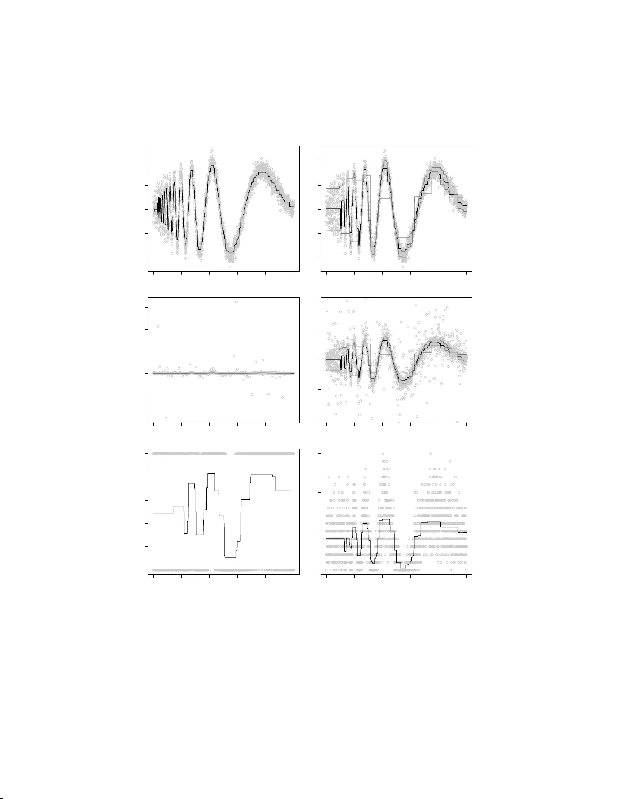
Electronic Journal of Stat istics V ol. 3 (2009) 41–75 ISSN: 1935-7524 DOI: 10.1214/ 08-EJS21 6 Extensions of smo othing via taut strings ∗ Lutz D ¨ um bgen † University of Bern Institute for Mathematic al Statistic s and A ctuarial Scienc e Al p ene ggstr aße 22 CH-3012 Bern e-mail: lutz.due mbgen@st at.unibe.ch Arne Ko v ac ‡ University of Bristol Dep artment of Mathematics University Walk Bristol BS8 1TW, UK e-mail: a.kovac@ bristol. ac.uk Abstract: Suppose that we observe independent random pairs ( X 1 , Y 1 ), ( X 2 , Y 2 ), . . . , ( X n , Y n ). Our goal is to estimate regressi on functions such as the conditional m ean or β –quantile of Y giv en X , where 0 < β < 1. In order to ac hiev e this we minimize criteria suc h as, for instance, n X i =1 ρ ( f ( X i ) − Y i ) + λ · TV ( f ) among al l candidate functions f . He re ρ is some con v ex function dep ending on the particular regression function we hav e in mind, TV( f ) stands for the total v ariation of f , and λ > 0 is s ome tuning parameter. This f rame- wo rk is exte nded further to include binary or Poisson regression, and to i n- clude locali zed total v ariation penalties. The latter are needed to construct estimators adapting to inhomogeneous smoothness of f . F or the general framework w e dev elop noniterativ e algorithms f or the solution of the m in- imization problems which are closely related to the taut str ing algori thm (cf. Da vies and Kov ac , 2001 ). F urther we establish a connection b et w een the presen t setting and monotone regression, extending previous work by Mammen and v an de Geer ( 1997 ). The algorithmic considerations and n u- merical examples are complemen ted by t w o consistenc y resul ts. AMS 2000 sub ject classi fications: Prim ary 62G 08; secondary 62G35. Keywords and phra ses: conditional means, conditional quantiles, mo dal- ity , p enalization, uniform consistency , total v ari ation, tube metho d. Receiv ed March 2008 . ∗ The authors thank Axel Munk and an Asso ciate Editor for constructiv e commen ts. † W ork supp orted by Swiss National Science F oundation ‡ W ork supp orted by Sonderforsc h ungsbereich 475, Unive rsity of Dortm und 41 L. D¨ umb gen and A . Kovac/Extensions of smo othing via taut strings 42 1. In troduction Suppos e that we observe pairs ( x 1 , Y 1 ), ( x 2 , Y 2 ), . . . , ( x n , Y n ) with fixed num b er s x 1 ≤ x 2 ≤ · · · ≤ x n and independent random v a riables Y 1 , Y 2 , . . . , Y n . W e assume that the distribution function of Y i depends on x i , i.e. P ( Y i ≤ z ) = F ( z | x i ) for s o me unknown family of distribution functions F ( · | x ), x ∈ R . O ften one is in terested in certain features of these distribution functions. Examples are the mean function µ with µ ( x ) := Z y F ( dy | x ) and, fo r so me β ∈ (0 , 1), the β –quantile function Q β , wher e Q β ( x ) is any nu mber z such that F ( z − | x ) ≤ β ≤ F ( z | x ) . This pap er treats estimation of such regression functions ut ilizing certa in roughness p enalties. The literature ab o ut p enalized regression estimators is v ast and still growing. As a go o d sta rting p oint we r ecommend An toniadis a nd F an ( 2001 ), v an de Geer ( 2001 ), Huang ( 2003 ), and the references ther ein. A first po ssibility is to minimize a functional of the form T ( f ) := n X i =1 ρ ( f ( x i ) − Y i ) + λ · TV( f ) (1) ov er all functions f on the real line. Here ρ is some con vex function measuring the size of the r esidual Y i − f ( x i ) and dep ending on the particular feature we hav e in mind . Moreov er, TV ( f ) denotes the total v aria tion o f f , tha t is the supremum of P m − 1 j =1 | f ( z j +1 ) − f ( z j ) | ov er all int egers m > 1 and num bers z 1 < z 2 < · · · < z m , while λ > 0 is some tuning parameter. Example I (m eans). In order to estimate the mean function µ , one c an take ρ ( z ) := z 2 / 2 . This pa rticular ca se has b een trea ted in detail b y Mammen and v an de Gee r ( 1997 ) and Davies a nd Kov ac ( 2001 ); see a ls o the remark following Lemma 2.2 . In pa r ticular, the latter authors describ e a n a lgorithm with r unning time O ( n ), the taut s tring metho d, to minimize the functional T ab ov e. Example I I (quantiles). F or the estimation o f a quantile function Q β one can take ρ ( z ) = ρ β ( z ) := | z | / 2 − ( β − 1 / 2) z = ( (1 − β ) z if z ≥ 0 , β | z | if z ≤ 0 . L. D¨ umb gen and A . Kovac/Extensions of smo othing via taut strings 43 Of par ticular interest is the case β = 1 / 2. Then ρ ( z ) = | z | / 2, and Q 1 / 2 is the conditional median function. This particula r functional has also b een s uggested b y Simpson, He and Liu in their discussion of Chu et a l. ( 19 98 ) but, as far as we know, not b een considered in mor e detail later o n. Howev er, similar functionals using a discretisation o f the total v ariation of the first deriv ativ e as a p e na lt y hav e b een studied b y Ko enker, Ng a nd Portnoy ( 1994 ) or in t w o dimensions by Ko enker and Mizer a ( 20 04 ). They employ linear pr ogra mming techniques like in terior po int metho ds to find solutions to the resulting minimisation pro blems. A primary go al of the present pap er is to ex tend the classical taut string algo - rithm to other situations such as Example I I, or binary and Poisson r e g ression. Compared to the linear prog ramming techniques mentioned ab ov e, the gener- alized taut string metho d has the a dv antage of b eing computationally fa s ter and more sta ble. In the sp ecific case of Exa mple I I it is po ssible to calculate a solution in time O ( n log ( n )). Note that the original algo rithm yields piecewise constant functions. O n each constant int erv al the function v alue is equal to the mean of the cor resp onding o bs erv a tio ns, except for lo cal extrema of the fit. I n their discussion of Davies and K ov ac ( 2001 ), Mammen a nd v an de Geer men- tion the pos sibilit y to replace sample means just by sample quantiles, in or der to trea t Example I I. How ever, the pres ent a uthors realized that the ex tension is not that straightforw ard. The r emainder o f this pap er is or ganized as follows: In Section 2 w e describ e an extension o f the function T ab ov e such that it cov ers als o other mo dels such a s binary and Poisson regressio n. In a ddition w e replace the p enalty term λ · T V ( f ) b y a more flexible roughness measur e which allows lo cal a daptation to v ar ying smo othness o f the under ly ing reg ression function. Then we derive necessary and sufficient conditions for a function ˆ f to minimize o ur functional. In that con text we als o esta blish a connection to monotone regressio n which is useful for un- derstanding adaptivity prop erties of the pro ce dur e. This generalizes findings of Mammen and v an de Geer ( 1997 ) for the least sq uares ca se. In Sec tio ns 3 and 4 we derive generalized taut string algor ithms, extending the algorithm describ ed b y Da vies and Kov ac ( 20 0 1 ). While Section 3 covers c o nti nuously differen tiable functions ρ , Section 4 is for gener al ρ a nd, in particular, Exa mple I I. Section 5 explains how our tuning para meter s, e.g. λ in ( 1 ), may b e chosen. Section 6 presents some numerical examples of our metho ds. In Section 7 we comple- men t the a lgorithmic considerations with tw o co nsistency results which a re of independent interest. One of them ent ails unifor m consistency of monotone r e- gression estimators, while the other applies to arbitrar y estimators such that the corr esp onding residuals s atisfy a certain multiscale criterion. Both res ults are a first step tow ards a detailed a symptotic a nalysis of taut string and rela ted methods . All longe r pro ofs are deferr e d to Section 8 . 2. The general se tting F or simplicit y we assume throughout this pap er that x 1 < x 2 < · · · < x n . In Section 3.3 we describ e briefly p ossible modifica tions to deal with p otential ties among the x i . L. D¨ umb gen and A . Kovac/Extensions of smo othing via taut strings 44 2.1. The tar get functional W e often iden tify a function f : R → R with the v ector f = ( f i ) n i =1 := ( f ( x i )) n i =1 . Our aim is to minimize functionals of the form T ( f ) = T λ ( f ) := n X i =1 R i ( f i ) + n − 1 X j =1 λ j | f j +1 − f j | ov er all vectors f ∈ R n , where λ ∈ (0 , ∞ ) n − 1 is a given vector of tuning pa ram- eters while the R i are random functions dep ending on the data. In general w e assume the fo llowing t wo conditions to b e s a tisfied: (A.1) F or each index i , the function R i : R → R is conv ex. (A.2) T is co ercive, i.e. T ( f ) → ∞ as k f k → ∞ . Condition (A.1) entails that T is a contin uous and c o nv ex functional on R n , so the additional Co ndition (A.2) guar antees the existence of a minimizer ˆ f of T . This will b e our estimator for the r egressio n function of interest, ev a luated a t the design p oints x i . The sp ecia l functional T in ( 1 ) corr esp onds to λ 1 = · · · = λ n − 1 = λ and R i ( z ) := ρ ( z − Y i ). Here our Conditions (A.1–2) are sa tisfied if ρ ( z ) → ∞ as | z | → ∞ . Two additiona l examples for R i follow. Example I I I (Poisson regressi on). Suppose that Y i ∈ { 0 , 1 , 2 , . . . } has a Poisson distribution with mean µ ( x i ) > 0, and let R i ( z ) := exp( z ) − z Y i . These functions a re strictly conv ex with R i ≥ Y i log( e/ Y i ). Thus T is even strictly c o nv ex, a nd elementary c o nsiderations reveal that it is co er cive if Y i > 0 for at least o ne index i . In that case w e end up with a unique penalized maximum likelih o o d estimator ˆ f o f log µ . Example IV (Bi nary regression). Similarly let Y i ∈ { 0 , 1 } with mean µ ( x i ) ∈ (0 , 1), a nd define R i ( z ) := − Y i z + log (1 + exp( z )) . Here R i > 0 , and aga in T is strictly conv ex. It is co er cive if the Y i are not a ll iden tical, and the minimizer ˆ f of T may b e viewed as a pena lized maximum likelih o o d estimator of logit( µ ) := log( µ/ (1 − µ )). 2.2. Char acterizations of the soluti on As mentioned before, Conditions (A.1–2) guarantee the ex istence of a minimizer ˆ f of T . In the present s ubsection we derive v a rious characterizations of such minimizers, assuming o nly Condition (A.1). L. D¨ umb gen and A . Kovac/Extensions of smo othing via taut strings 45 By c o nv exit y o f T , a vector ˆ f ∈ R n minimizes T if, and o nly if, all directional deriv atives a t ˆ f are non-negative, i.e. D T ( ˆ f , δ ) := lim ε ↓ 0 T ( ˆ f + ε δ ) − T ( ˆ f ) ε ≥ 0 for any δ ∈ R n . (2) More sp ecifically , let R ′ i ( z ± ) b e the left- and right-sided deriv ativ es o f R i at z , i.e. R ′ i ( z ± ) := lim ε ↓ 0 R i ( z ± ε ) − R i ( z ) ± ε . Then D T ( ˆ f , δ ) equals X i : δ i > 0 R ′ i ( ˆ f i +) δ i + X i : δ i < 0 R ′ i ( ˆ f i − ) δ i + n − 1 X j =1 λ j  sign( ˆ f j +1 − ˆ f j )( δ j +1 − δ j ) + 1 { ˆ f j +1 = ˆ f j }| δ j +1 − δ j |  , where 1 { . . . } denotes the indicator function. Plugging in v arious sp ecia l vectors δ reveals v aluable informa tion a bo ut min- imizers ˆ f . In particular , for indices 1 ≤ j ≤ k ≤ n let δ ( j k ) :=  1 { j ≤ i ≤ k }  n i =1 . Then D T ( ˆ f , + δ ( j k ) ) = k X i = j R ′ i ( ˆ f i +) − λ j − 1 sign ( ˆ f j − 1 − ˆ f j ) − λ k sign( ˆ f k +1 − ˆ f k ) , D T ( ˆ f , − δ ( j k ) ) = − k X i = j R ′ i ( ˆ f i − ) + λ j − 1 sign( ˆ f j − 1 − ˆ f j ) + λ k sign( ˆ f k +1 − ˆ f k ) . Here sign ( z ) := 1 { z > 0 } − 1 { z ≤ 0 } and sig n( z ) := 1 { z ≥ 0 } − 1 { z < 0 } , and throughout this pap e r we s et v 0 := v m +1 := 0 for any v ector v = ( v i ) m i =1 ∈ R m . In particular, λ 0 := λ n := 0. Consequently , applying ( 2 ) to ± δ ( j k ) yields the key inequalities k X i = j R ′ i ( ˆ f i +) ≥ λ j − 1 sign ( ˆ f j − 1 − ˆ f j ) + λ k sign( ˆ f k +1 − ˆ f k ) and k X i = j R ′ i ( ˆ f i − ) ≤ λ j − 1 sign( ˆ f j − 1 − ˆ f j ) + λ k sign( ˆ f k +1 − ˆ f k ) . (3) These considera tions yield already o ne part of the followin g result. Lemma 2. 1 A ve ctor ˆ f ∈ R n minimizes T if, and only if, ( 3 ) holds for al l 1 ≤ j ≤ k ≤ n . L. D¨ umb gen and A . Kovac/Extensions of smo othing via taut strings 46 In case of differe ntiable functions R i there is a s impler characterizatio n of a minimizer of T : Lemma 2. 2 Supp ose that al l functions R i ar e differ entiable on R . Then a ve c- tor ˆ f ∈ R n minimizes T if, and only if, for 1 ≤ k ≤ n , k X i =1 R ′ i ( ˆ f i )    ∈ [ − λ k , λ k ] , = λ k if k < n and ˆ f k < ˆ f k +1 , = − λ k if k < n and ˆ f k > ˆ f k +1 . (4) F or k = n , it follows from λ n = 0 that Condition ( 4 ) amounts to n X i =1 R ′ i ( ˆ f i ) = 0 . Note that in the classical case, R i ( z ) = ( z − Y i ) 2 / 2 and P k i =1 R ′ i ( ˆ f i ) = P k i =1 ˆ f i − P k i =1 Y i . Thus our result entails Mammen and v a n de Geer’s ( 1997 ) finding that the solution ˆ f may b e r e pr esented as the der iv ative o f a taut string co nnecting the p oints (0 , 0) and  n, P n i =1 Y i  and forced to lie within a tube centered at the p oints  k , P k i =1 Y i  , 1 ≤ k < n . In the gener al s e tting treated here, there ar e no longer taut strings , but the solutions can still b e characterized by a tub e. This is illustrated in the left panels of Figure 1 with a sma ll example. The upp er panel shows a da ta set of size n = 25 (with x i = i ) and the approximation ˆ f obtained fro m the functional T in ( 1 ) with ρ ( z ) := √ 0 . 1 2 + z 2 and λ = 2. This function ρ ( r ) may b e viewed as a smo othed version of | z | with R ′ i ( z ) = z − Y i p 0 . 1 2 + ( z − Y i ) 2 being similar to sign( z − Y i ). The low er panel s hows the cumulativ e sums of the “residuals” R ′ i ( ˆ f i ). As predicted by Lemma 2.2 , these sums are alwa ys b etw een − λ and λ , and they touch these b oundaries whenev er the v a lue of ˆ f changes. 2.3. Boundi ng the r ange of the soluti ons Sometimes it is helpful to know a priori so me bo unds for any minimizer ˆ f of T . W e start with a rather obvious fa c t: Suppo se that there are num bers z ℓ < z r such that fo r i = 1 , . . . , n , R ′ i ( z +) < 0 if z < z ℓ , R ′ i ( z − ) > 0 if z > z r . Then any minimizer of T belo ng s to [ z ℓ , z r ] n . F or if f ∈ R n \ [ z ℓ , z r ] n , one can easily verify that replacing f with  min(max( f i , z ℓ ) , z r )  n i =1 yields a strictly smaller v a lue o f T ( f ). In case of differentiable functions R i an even stro nger statement is tr ue: L. D¨ umb gen and A . Kovac/Extensions of smo othing via taut strings 47 5 10 15 20 25 −3 −2 −1 0 1 2 0 5 10 15 20 25 −2 −1 0 1 5 10 15 20 25 −3 −2 −1 0 1 2 0 5 10 15 20 25 −2 −1 0 1 2 Fig 1 . Il lustr ation of L emma 2.2 and Conditions (C.1 K ) and (C.2 f & g ,K ) of A lgorithm I. Lemma 2. 3 Supp ose that the functions R i ar e differ entiable su ch t hat for c er- tain numb ers z ℓ < z r , R ′ i ( z ℓ ) ≤ 0 for al l i with at le ast one strict ine quality , R ′ i ( z r ) ≥ 0 for al l i with at le ast one strict ine quality . Then any minimizer of T is c ontaine d in ( z ℓ , z r ) n . In the sp ecial case of R i ( z ) = ρ ( z − Y i ) we reach the following co nclusions: If 0 is the unique minimizer o f ρ ov er R , then a ny minimizer of T b elong s to  min( Y 1 , . . . , Y n ) , max( Y 1 , . . . , Y n )  n . If in addition ρ is differentiable and Y = ( Y i ) n i =1 is non- c o nstant, then any minimizer of T b elo ngs even to  min( Y 1 , . . . , Y n ) , max( Y 1 , . . . , Y n )  n . 2.4. A link to monotone r e gr ession An interesting a lternative to smo othness assumptions a nd roughness p enalties is to assume mo notonicity of the underlying regres sion function f on certain in terv als . F or ins ta nce, if f is assumed to b e isoto nic, one could determine an L. D¨ umb gen and A . Kovac/Extensions of smo othing via taut strings 48 estimator ˇ f minimizing P n i =1 R i ( ˇ f i ) under the co ns traint that ˇ f 1 ≤ ˇ f 2 ≤ · · · ≤ ˇ f n . The next theorem shows that our p enalized estimators ˆ f often coincide lo cally with mo notone estimators . Theorem 2 . 4 Supp ose t hat 1 < a ≤ b < n such t hat λ a − 1 = λ a = · · · = λ b and ˆ f a − 1 < ˆ f a ≤ · · · ≤ ˆ f b < ˆ f b +1 . Then ( ˆ f i ) b i = a minimizes P b i = a R i ( f i ) among al l ve ctors ( f i ) b i = a satisfying f a ≤ · · · ≤ f b . An analo gous statement holds for antitonic fits. 3. Computation in case of regul ar functions R i 3.1. A gener al algorithm for str ongly c o er cive functions R i In this subsection we presen t a n algorithm for the minimization of the functional T in case of (A.1) together with the additional co nstraint that (A.3) all functions R i are contin uously differe ntiable with lim z →−∞ R ′ i ( z ) = −∞ and lim z →∞ R ′ i ( z ) = ∞ . Obviously the la tter condition is s atisfied in E x ample I. Note that Co nditions (A.1) and (A.3) imply Condition (A.2). Mo r eov er, R ′ i : R → R is iso tonic (i.e. non-decreasing ), contin uous and surjective. The algorithm’s principle. The idea o f our algorithm is to compute induc- tiv ely for K = 1 , 2 , . . . , n a vector ( ˆ f i ) K i =1 such that Co ndition ( 4 ) holds for 1 ≤ k ≤ K , where ˆ f K + 1 may b e defined arbitrar ily . Precisely , inductiv ely for K = 1 , 2 , . . . , n we co mpute two candidate vectors f = ( f i ) K i =1 and g = ( g i ) K i =1 in R K such that at the end o f step K the following three conditions ar e satisfied: (C.1 K ) There exists an index k o = k o ( f , g ) ∈ { 0 , 1 , . . . , K } s uch that g i − f i ( = 0 for 1 ≤ i ≤ k o , > 0 for k o < i ≤ K. Moreov er, f i is a nt itonic (i.e. non-increa sing) and g i is is o tonic in i ∈ { k o + 1 , . . . , K } . (C.2 g,K ) F or 1 ≤ k ≤ K , k X i =1 R ′ i ( g i ) ≤ λ k with equality if ( k < K and g k < g k +1 , k = K. (C.2 f ,K ) F or 1 ≤ k ≤ K , k X i =1 R ′ i ( f i ) ≥ − λ k with eq ua lit y if ( k < K and f k > f k +1 , k = K. L. D¨ umb gen and A . Kovac/Extensions of smo othing via taut strings 49 Note that Conditions (C.1 K ) and (C.2 f & g ,K ) imply the following fact: (C.3 K ) Let Λ o = Λ o ( f , g ) := P k o i =1 R ′ i ( f i ). If 1 ≤ k o < K , then either f k o = g k o ≥ g k o +1 > f k o +1 and Λ o = − λ k o , or g k o = f k o ≤ f k o +1 < g k o +1 and Λ o = λ k o . When the a lgorithm finishes with K = n , a s o lution ˆ f ∈ R n may be obtained as follows: If k o = n , ˆ f := f = g satisfies the conditions of Le mma 2.2 . If k o < n , w e define ˆ f i := ( f i = g i for 1 ≤ i ≤ k o r for k o < i ≤ n with s ome num ber r ∈ [ f k o +1 , g k o +1 ]. This definition en tails that f i ≤ ˆ f i ≤ g i for all indices i , while ˆ f i is constant in i > k o . Hence one can easily deduce from Conditions (C.2 f & g ,n ) that ˆ f satisfies the conditions of Lemma 2.2 . T o ensure a certain o ptimalit y prop erty des crib ed later, in case of 1 ≤ k o < n w e choose r := ( g k o +1 if f k o = g k o ≥ g k o +1 , f k o +1 if g k o = f k o ≤ f k o +1 . Conditions (C.1 K ) and (C.2 f & g ,K ) a re illustrated in the r ight panels of Fig- ure 1 which show the same example as the left pa nels that were discussed in the previous Section. Strictly sp eaking, Condition (A.3) is not s a tisfied her e, but one can enforce it by a dding min( z − c 1 , 0) 2 + max( z − c 2 , 0) 2 to R i ( z ) = ρ ( z − Y i ) with arbitra ry constants c 1 ≤ min( Y 1 , . . . , Y n ) and c 2 ≥ max( Y 1 , . . . , Y n ). This mo dification do es not alter the s olution which is contained in [ c 1 , c 2 ] n ; see Sec- tion 2.3 . The solid and grey lines in the upper panel represent f a nd g , resp ectively , where K = 20 and k o = 3. The low er panel shows the corresp onding cum ulative sums of the n um ber s R ′ i ( f i ) and R ′ i ( g i ), 1 ≤ i ≤ K . Some auxiliary functions and te rm i nology . Later on we shall w ork with partitions of the s et { 1 , 2 , . . . , n } into index interv als and functions (vectors) which are constant on these int erv a ls. T o define the latter vectors efficiently we define R ′ j k := k X i = j R ′ i for indices 1 ≤ j ≤ k ≤ n . Ag ain, R ′ j k is contin uo us a nd isotonic on R with limits R ′ j k ( ±∞ ) = ±∞ . F urther, for re a l num b er s t let M j k ( t ) := min  z ∈ R : R ′ j k ( z ) ≥ t  , M j k ( t ) := max  z ∈ R : R ′ j k ( z ) ≤ t  . L. D¨ umb gen and A . Kovac/Extensions of smo othing via taut strings 50 These quant ities M j k ( t ) and M j k ( t ) are iso tonic in t , where R ′ j k ( z ) = t for any real num b er z ∈  M j k ( t ) , M j k ( t )  . The following lemma summarizes basic prop erties of the a uxiliary functions M j k which ar e essential for Algorithm I below. The functions M j k satisfy ana l- ogous prop erties. Lemma 3. 1 L et 1 ≤ j ≤ k < ℓ ≤ m ≤ n b e indic es with ℓ = k + 1 . F u rt her let c, u, v ∈ R such that R ′ j k ( c ) = u. (a) If c ≥ M ℓm ( v ) , then c ≥ M j m ( u + v ) ≥ M ℓm ( v ) . (b) If c > M j m ( u + v ) , t hen M j m ( u + v ) ≥ M ℓm ( v ) . F or some vector v = ( v i ) b i = a , a maximal index interv al J ⊂ { a , . . . , b } such that v i is cons tant in i ∈ J will b e called a “se g ment of v ”. Algorithm I: Step 1 . F or K = 1 we define f 1 := M 1 , 1 ( − λ 1 ) and g 1 := M 1 , 1 ( λ 1 ) . Conditions (C.1 1 ) and (C.2 f & g , 1 ) are certainly satisfied. Algorithm I: Step K + 1. Supp ose that Conditions (C.1 K ) and (C.2 f & g ,K ) are sa tisfied for some K ∈ { 1 , . . . , n − 1 } . Since λ K > 0, one can easily derive from (C.2 f & g ,K ) that k o < K . Subsequently we constr uct new ca ndidates ˜ f = ( ˜ f i ) K + 1 i =1 for f and ˜ g = ( ˜ g i ) K + 1 i =1 for g . In this context, (C.1 K + 1 ) and (C.2 ··· ,K +1 ) alwa ys denote conditions on the new vectors ˜ f and ˜ g in place of f and g , resp ectively , while (C.1 K ) and (C.2 ··· ,K ) refer to the origina l f a nd g . Initializing ˜ g . W e set ˜ g i := ( g i for i ≤ K , M K + 1 ,K +1 ( λ K + 1 − λ K ) for i = K + 1 . Since ˜ g i = g i for all i ≤ K , one can easily verify that the inequa lit y part of (C.2 g,K +1 ) is sa tisfied, a nd also P K + 1 i =1 R ′ i ( ˜ g i ) = λ K + 1 . Mo difying ˜ g . Suppo se that ˜ g i is not isotonic in i > k o . By the previous construction of ˜ g , this mea ns that the tw o rig ht most segments { j, . . . , k } and { ℓ, . . . , K + 1 } of ( ˜ g i ) K + 1 i = k o +1 satisfy ˜ g k > ˜ g ℓ , where k o < j ≤ k = ℓ − 1 ≤ K . In that case we replace ˜ g i , i ∈ { j, . . . , K + 1 } , w ith ( M j,K +1 ( λ K + 1 − λ j − 1 ) if j > k o + 1 , M j,K +1 ( λ K + 1 − Λ o ) if j = k o + 1 . L. D¨ umb gen and A . Kovac/Extensions of smo othing via taut strings 51 This step is rep eated, if necessa ry , until ˜ g i is isotonic in i > k o . O ne can easily de- duce from Part (a) o f Lemma 3.1 b elow that thro ug hout ˜ g i ≤ g i for k o < i ≤ K while P K + 1 i =1 R ′ i ( ˜ g i ) = λ K + 1 . Hence the inequa lit y part of Condition (C.2 g,K +1 ) contin ues to hold. The equality statement s of Condition (C.2 g,K +1 ) are true as well, the only p ossible exception b eing k = k o . This exceptional case may o ccur only if ˜ g k o +1 < g k o +1 , and by our construction of ˜ g , this entails ˜ g i being constant in i ∈ { k o + 1 , . . . , K + 1 } . Initializing ˜ f . W e set ˜ f i := ( f i for i ≤ K , M K + 1 ,K +1 ( − λ K + 1 + λ K ) for i = K + 1 . Again the inequality pa rt of (C.2 f ,K +1 ) is satisfied, and also P K + 1 i =1 R ′ i ( ˜ f i ) = − λ K + 1 . Mo difying ˜ f . Supp ose that ˜ f i is not a nt itonic in i > k o . This means that the t wo right most seg ments { j, . . . , k } and { ℓ, . . . , K + 1 } of ( ˜ f i ) K + 1 i = k o +1 satisfy ˜ f k < ˜ f ℓ , where k o < j ≤ k = ℓ − 1 ≤ K . In tha t ca se we r eplace ˜ f i , i ∈ { j, . . . , K + 1 } , with ( M j,K +1 ( − λ K + 1 + λ j − 1 ) if j > k o + 1 , M j,K +1 ( − λ K + 1 − Λ o ) if j = k o + 1 . This step is rep eated, if necessar y , until ˜ f i is antitonic in i > k o . Thro ughout, ˜ f i ≥ f i for k o < i ≤ K while P K + 1 i =1 R ′ i ( ˜ f i ) = − λ K + 1 . Hence the inequality part of Condition (C.2 f ,K +1 ) contin ues to b e sa tisfied. The equality statements of Condition (C.2 f ,K +1 ) are true as well, the only p oss ible exception being k = k o . This exceptiona l cas e ma y o cc ur only if ˜ f k o +1 > f k o +1 , and this entails that ˜ f i is constant in i > k o . This s tep is illustrated in Figure 2 which shows again the example fro m Figure 1 . Here K = 17 and the panels show from left to right the initialisa tion of ˜ f , the first mo dification of ˜ f and the se c o nd and final mo dification. The panels in the upp er row show the data and the approximations while the panels in the lower r ow show the corresp onding cumulativ e sums of the num b ers R ′ i ( f i ) and R ′ i ( g i ), 1 ≤ i ≤ K . Final mo dification of ˜ f and ˜ g . Having completed the previo us co nstruc- tion, we end up with vect ors ˜ f and ˜ g satisfying the inequa lity pa rts of Con- ditions (C.2 f & g ,K +1 ). The equalit y parts ar e satisfied as well, with p ossible exceptions only for k = k o ( f , g ). Moreover, ˜ f i is antitonic and ˜ g i is isotonic in i > k o . Finally , our explicit construction entails tha t f k o +1 = ˜ f k o +1 or f k o +1 < ˜ f k o +1 = · · · = ˜ f K + 1 , and g k o +1 = ˜ g k o +1 or g k o +1 > ˜ g k o +1 = · · · = ˜ g K + 1 . L. D¨ umb gen and A . Kovac/Extensions of smo othing via taut strings 52 0 10 20 30 40 50 −4 −3 −2 −1 0 1 2 3 0 10 20 30 40 50 −2 −1 0 1 2 0 10 20 30 40 50 −4 −3 −2 −1 0 1 2 3 0 10 20 30 40 50 −2 −1 0 1 2 0 10 20 30 40 50 −4 −3 −2 −1 0 1 2 3 0 10 20 30 40 50 −2 −1 0 1 2 Fig 2 . Il lustr ation of the mo dific ation step for ˜ f in Algorithm I. Suppos e first that ˜ f k o +1 ≤ ˜ g k o +1 . Then one ca n ea s ily deduce fro m (C.3 K ) and the prop erties of ˜ f , ˜ g just ment ioned that Conditions (C.1 K + 1 ) and (C.2 f & g ,K +1 ) are satisfied. One pa rticular instance of the previo us situation is that b oth ˜ f i and ˜ g i are constant in i > k o . F or then − λ K + 1 = K + 1 X i =1 R ′ i ( ˜ f i ) = Λ o + R ′ k o +1 ,K +1 ( ˜ f k o +1 ) and λ K + 1 = K + 1 X i =1 R ′ i ( ˜ g i ) = Λ o + R ′ k o +1 ,K +1 ( ˜ g k o +1 ) . Now supp ose that ˜ f k o +1 > ˜ g k o +1 . The previous consideratio ns and our con- struction of ˜ f and ˜ g show that either ˜ f K + 1 < ˜ f k o +1 = f k o +1 > ˜ g k o +1 , or ˜ g K + 1 > ˜ g k o +1 = g k o +1 < ˜ f k o +1 . L. D¨ umb gen and A . Kovac/Extensions of smo othing via taut strings 53 W e discuss only the former case, the latter case being handled analog o usly . Here Condition (C.2 f ,K +1 ) is satisfied already . Let { k o + 1 , . . . , k 1 } b e the leftmost segment of ( ˜ f i ) K + 1 i = k o +1 . Then w e redefine ˜ g as follows: ˜ g i :=      f i = g i for i ≤ k o , ˜ f k o +1 for k o < i ≤ k 1 , M k 1 +1 ,K +1 ( λ K + 1 + λ k 1 ) for k 1 < i ≤ K + 1 . By as s umption, R ′ k o +1 ,k 1 ( ˜ f k o +1 ) = − λ k 1 − Λ o and M k o +1 ,K +1 ( λ K + 1 − Λ o ) < ˜ f k o +1 . Hence Part (b) of Lemma 3.1 entails that the new v a lue of ˜ g k 1 +1 is not greater than M k o +1 ,K +1 ( λ K + 1 − Λ o ), w hich is the old v alue o f ˜ g k o +1 = · · · = ˜ g K + 1 . Since ˜ f k o +1 = f k o +1 < g k o +1 , we may conclude that the new vector ˜ g still sa tisfies ˜ g i < g i for k o < i ≤ K . Now one easily verifies that the new vector ˜ g satisfies Condition (C.2 g,K +1 ). It may happ en that Condition (C.1 K + 1 ) is still violated, i.e. ˜ g k 1 +1 < ˜ f k 1 +1 . In that case we r epe a t the previous up date of ˜ g with k 1 in place of k o and iterate this pro cedur e until Condition (C.1 K + 1 ) is sa tisfied as well. This s tep is illustr ated in Figure 3 which shows once more the example from Figure 1 a nd 2 . Her e K = 23 and the left panels show ˜ f befo r e the final mo difi- cation while the result of the mo difica tion is shown in the right pa nel. As alwa ys 0 10 20 30 40 50 −4 −3 −2 −1 0 1 2 3 0 10 20 30 40 50 −2 −1 0 1 2 0 10 20 30 40 50 −4 −3 −2 −1 0 1 2 3 0 10 20 30 40 50 −2 −1 0 1 2 Fig 3 . Il lustr ation of the final mo dific ation st ep for ˜ f in Algorithm I. L. D¨ umb gen and A . Kovac/Extensions of smo othing via taut strings 54 the panels in the upp er row show the data and the approximations while the panels in the low er row show the corr esp onding cum ulativ e sums of the num bers R ′ i ( f i ) and R ′ i ( g i ), 1 ≤ i ≤ K . An optimality prop erty of Algorithm I. The solution ˆ f pro duced by Algorithm I is as simple a s p ossible in a cer ta in sense. F o r a vector f ∈ R n , an index int erv a l { j, . . . , k } ⊂ { 1 , 2 , . . . , n } with j > 1 or k < n is called a    lo cal ma ximum of f if f j = · · · = f k > max i ∈N f i , lo cal minimum of f if f j = · · · = f k < min i ∈N f i , where N := { j − 1 , k + 1 } ∩ { 1 , 2 , . . . , n } . Theorem 3 . 2 L et ˆ f b e t he ve ctor pr o duc e d by Algorithm I, and let f b e any ve ctor in R n such that      k X i =1 R ′ i ( f i )      ≤ λ k for 1 ≤ k ≤ n . (5) Then max i ∈J f i ≥ ma x i ∈J ˆ f i for any lo c al maximum J of ˆ f , min i ∈J f i ≤ min i ∈J ˆ f i for any lo c al minimum J of ˆ f . In particular the theore m shows that every vector f satisfying the tub e con- dition ( 5 ) must have at lea st the sa me num b er of lo cal ex tr eme v alues as ˆ f . 3.2. Exp onential families Examples I I I a nd IV may b e generalized as follows: Supp ose that Y j has dis- tribution P f ( x j ) for some unknown r eal parameter f ( x j ), where ( P θ ) θ ∈ R is an exp o nential family with dP θ dν ( y ) = exp  θy − b ( θ )  for some mea sure ν on the real line. In case of Poisson regre s sion, ν is a discrete measure o n { 0 , 1 , 2 , . . . } with weigh ts ν ( { k } ) = 1 /k !, so that b ( θ ) = b ′ ( θ ) = b ′′ ( θ ) = e θ . F o r binomial regr ession we choose ν to b e co unt ing measur e on { 0 , 1 } , whence b ( θ ) = lo g(1 + e θ ), b ′ ( θ ) = e θ / (1 + e θ ) and b ′′ ( θ ) = b ′ ( θ )(1 − b ′ ( θ )). Note that in gener al, b ( · ) is infinitely often differentiable with b ′ ( θ ) and b ′′ ( θ ) being the mean a nd v a riance, resp ectively , of the distribution P θ . W e a ssume that b ′′ ( θ ) is strictly p ositive for all θ ∈ R . Note also that ν ( R \ [ y min , y max ]) = 0, where y min and y max are the infim um and supremum, resp ectively , of the set  b ′ ( θ ) : θ ∈ R  . L. D¨ umb gen and A . Kovac/Extensions of smo othing via taut strings 55 Now we consider minimization of minus the log -likelihoo d function plus the lo calized total v ariation p enalty , i.e. R i ( z ) := b ( z ) − z Y i . By assumption, these functions ar e infinitely o ften different iable with first deriv a- tiv e R ′ i ( z ) = b ′ ( z ) − Y i and strictly p ositive second deriv ative R ′′ i ( z ) = b ′′ ( z ). Hence they satisfy Condition (A.1). Unfortunately they may fail to b e co ercive individually , a nd Condition (A.3) is not satisfied in general. How ever, one can show that Co ndition (A.2) is satisfied a s so o n as Y is non-trivia l in the sense that min( Y 1 , . . . , Y n ) < ma x( Y 1 , . . . , Y n ) . (6) W e will not pursue this here, b ecause there is a simple solution of our estimation problem, at least in case of ( 6 ): A t firs t we apply the usual ta ut string metho d to the observ a tions Y i , i.e. we replace R i ( z ) with ρ ( z − Y i ), where ρ ( z ) := z 2 / 2. Let ˆ f LS be the resulting lea st squares fit. It follows from Lemma 2.3 that { ˆ f LS 1 , . . . , ˆ f LS n } ⊂  min( Y 1 , . . . , Y n ) , max( Y 1 , . . . , Y n )  . Thu s the vector ˆ f with comp onents ˆ f i := ( b ′ ) − 1 ( ˆ f LS i ) is well-defined and satisfies P k i =1 R ′ i ( ˆ f i ) = P k i =1 ρ ′ ( ˆ f LS i − Y i ). Hence a pplying Lemma 2.2 to ˆ f LS in the least squares setting entails the analo gous co nditions for ˆ f in the max im um likelihoo d setting. This shows that ˆ f is indeed the unique minimizer of T . 3.3. Ties among the x i F or simplicit y w e a ssumed that x 1 < x 2 < · · · < x n . Now we r elax this assump- tion temp ora r ily to x 1 ≤ x 2 ≤ · · · ≤ x n and descr ibe a poss ible mo dification of Algorithm I. Let x (1) < x (2) < · · · < x ( m ) be the distinct elements of { x 1 , x 2 , . . . , x n } , and let i ( k ) := ma x { i : x i = x ( k ) } . Then we restrict our attent ion to vectors f ∈ R n such that f i = f j for i ( k − 1) < i < j ≤ i ( k ), 1 ≤ k ≤ m , where i (0) := 0. The target functional has to b e r ewritten as T ( f ) = n X i =1 R i ( f i ) + m − 1 X k =1 λ j | f i ( k +1) − f i ( k ) | . Now Algor ithm I uses induction on K = 1 , 2 , . . . , m . In Step 1 we define f i := M 1 ,i (1) ( − λ 1 ) and g i := M 1 ,i (1) ( λ 1 ) for 1 ≤ i ≤ i (1) . L. D¨ umb gen and A . Kovac/Extensions of smo othing via taut strings 56 In Step K + 1 we aim for vectors ˜ f and ˜ g in R i ( K +1) . The initial versions are given by ˜ g i := ( g i for i ≤ i ( K ) , M i ( K )+1 ,i ( K +1) (+ λ K + 1 − λ K ) for i ( K ) < i ≤ i ( K + 1) , ˜ f i := ( f i for i ≤ i ( K ) , M i ( K )+1 ,i ( K +1) ( − λ K + 1 + λ K ) for i ( K ) < i ≤ i ( K + 1) , while the remainder of Step K + 1 remains unchanged. 4. The case o f arbitrary functions R i In this Section we describ e how to calculate s olutions to the gener a l s etting describ ed in Section 2 . In particular we investigate how to solve the quantile regress io n problem presented in Example I I. Throughout this s ection we assume that Conditions (A.1– 2 ) ar e s a tisfied, while so me o f the functions R i may fail to satisfy the regularity condition (A.3). 4.1. Appr oximating the R i W e sta rt with a g eneral observ ation: F or ε > 0 a nd i ∈ { 1 , 2 , . . . , } let R i,ε : R → R b e a (data -driven) conv ex function such that lim ε ↓ 0 R i,ε ( z ) = R i ( z ) fo r any z ∈ R . (7) The corresp onding approximation T ε ( f ) = T λ ,ε ( f ) to T ( f ) equals P n i =1 R i,ε ( f i )+ P n − 1 j =1 λ j | f j +1 − f j | and has the following pro per ties: Theorem 4 . 1 F or sufficiently smal l ε > 0 , the set ˆ F ε := arg min f ∈ R n T ε ( f ) is nonvoid and c omp act. Mor e over, it appr oximates the set ˆ F := arg min f ∈ R n T ( f ) in the sense that max f ε ∈ ˆ F ε min f ∈ ˆ F k f ε − f k → 0 as ε ↓ 0 . If we find a pproximations R i,ε satisfying additionally Condition (A.3), we can minimize the ta rget functional T ( · ) at least approximately by means of Algorithm I. O ne p ossible definition of such functions R i,ε is given by R i,ε ( z ) := 1 2 ε Z z + ε z − ε R i ( t ) dt + max( z − 1 /ε, 0) 2 2 + min( z + 1 /ε, 0) 2 2 . Here one can easily verify ( 7 ) and Co ndition (A.3) with R i,ε in place o f R i . L. D¨ umb gen and A . Kovac/Extensions of smo othing via taut strings 57 4.2. A non-iter ati ve solu tion for Example II Apparently the prece ding considerations lead to an iterative pro cedur e for min- imizing T . But such a detour is not alwa ys necessary . In this section w e de- rive an explicit combinatorial algo r ithm for Example I I. Recall that for given Y = ( Y i ) n i =1 , our go al is to minimize T ( f ) with R i ( z ) := ρ β ( z − Y i ). No te first that R ′ i ( z +) = 1 { Y i ≤ z } − β a nd R ′ i ( z − ) = 1 { Y i < z } − β . This indicates already that for quant ile regressio n mainly the ranks of the vector Y matter. Precisely , we shall work with a p e r mut ation Z = ( Z i ) n i =1 of ( i ) n i =1 such that # { i : Y i < Y j } + 1 ≤ Z j ≤ # { i : Y i ≤ Y j } for 1 ≤ j ≤ n. (8) That mea ns, Z is a rank vector of Y but without the usual mo dification in case of ties. The usefulness of this will b ecome clear la ter . Solving the original problem with Z in place of Y w o uld not b e muc h easier . But now we r e pla ce ρ β ( z − Z i ) with a smo oth function ˜ R i ( z ) such that ˜ R ′ i ( z ) =                z − β if z ≤ 0 , − β if 0 ≤ z ≤ Z i − 1 , z − Z i + 1 − β if Z i − 1 ≤ z ≤ Z i , 1 − β if Z i ≤ z ≤ n, z − n + 1 − β if z ≥ n ; see also Figure 4 . The idea behind ˜ R i is to replace ρ β ( z − Z i ) with R Z i Z i − 1 ρ β ( z − t ) dt , which w ould result in the deriv ative min  max( z − Z i + 1 − β , − β ) , 1 − β  . The e x tra mo difica tions on ( −∞ , 0) and ( n, ∞ ) are just to e ns ure the s trong co ercivity part o f Condition (A.3). Th us we pr op ose to minimize ˜ T ( g ) := n X i =1 ˜ R i ( g i ) + n − 1 X j =1 λ j | g j +1 − g j | b y means of Algorithm I a nd then to utilize the following result. Theorem 4 . 2 Supp ose that ˆ g minimizes ˜ T over R n . Then ˆ g ∈ ( β , n − 1 + β ) n . F urthermor e, let ˆ f ∈ R n b e given by ˆ f i := Y  ⌈ ˆ g i ⌉  with t he or der statistics Y (1) ≤ Y (2) ≤ · · · ≤ Y ( n ) of Y and ⌈ a ⌉ denoting the smal lest int e ger not smal ler than a ∈ R . Then ˆ f minimizes T over R n . L. D¨ umb gen and A . Kovac/Extensions of smo othing via taut strings 58 Fig 4 . The derivative ˜ R ′ i . Algorithm I I. Summarizing the preceding findings, we may compute the estimated β -quantile function by means of Algorithm I, applied to the functions ˜ R ′ i in place of R ′ i . Let us just comment on the cor resp onding a uxiliary functions ˜ M j k ( t ) := min  z ∈ R : ˜ R ′ j k ( z ) ≥ t  , ˜ M j k ( t ) := max  z ∈ R : ˜ R ′ j k ( z ) ≤ t  . If z (1) < z (2) < · · · < z ( ℓ ) are the ℓ := k − j + 1 order statistics o f ( Z i ) k i = j , then R ′ j k ( z ) =          ℓ min( z , 0) − ℓβ if z ≤ z (1) − 1 , i + z − z ( i ) − ℓβ if z ( i ) − 1 ≤ z ≤ z ( i ) , 1 ≤ i ≤ ℓ, i − ℓβ if z ( i ) ≤ z ≤ z ( i +1) − 1 , 1 ≤ i < ℓ , ℓ (1 − β + max ( z − n, 0 )) if z ≥ z ( ℓ ) . This entails that ˜ M j k ( t ) =      t/ℓ + β if t ≤ − ℓβ , z ( i ) + t − i + ℓβ if i − 1 − ℓβ < t ≤ i − ℓ β , 1 ≤ i ≤ ℓ, n + t/ℓ − 1 + β if t > ℓ (1 − β ) , ˜ M j k ( t ) =      t/ℓ + β if t < − ℓβ , z ( i ) + t − i + ℓβ if i − 1 − ℓβ ≤ t < i − ℓ β , 1 ≤ i ≤ ℓ, n + t/ℓ − 1 + β if t ≥ ℓ (1 − β ) . L. D¨ umb gen and A . Kovac/Extensions of smo othing via taut strings 59 T o implemen t this a lgorithm efficiently , one should use tw o additional vector v aria bles Z ( f ) and Z ( g ) such that for each segment { j, . . . , k } of f (resp. g ), ( Z ( f ) i ) k i = j (resp. ( Z ( g ) i ) k i = j ) contains the order statistics of ( Z i ) k i = j . Whenever t wo segments of f (resp. g ) are merged, the vector Z ( f ) (resp. Z ( g ) ) may b e upda ted by a suitable version o f Mer geSort ( Knut h , 1998 ). 5. The c hoice of tuning parameters λ j 5.1. Constant and fixe d λ Let us first discuss the simple case of a consta nt v alue λ > 0 for all λ j . In Example I, let ˆ σ b e s o me co nsistent estimato r of the standard devia tion of the v aria bles Y i , a ssuming tempora rily homo scedastic er rors Y i − µ ( x i ). F or instance, ˆ σ could b e the estimator prop osed by Rice ( 1984 ) or the version ba sed on the MAD b y Donoho et al. ( 1995 ). Since R ′ i ( z ) = z − Y i , and since for la rge n the pro cess [0 , 1] ∋ t 7→ n − 1 / 2 ˆ σ − 1 / 2 X i ≤ nt ( µ ( x i ) − Y i ) behaves similar ly as a standard Brownian motion b y vir tue of Donsker’s inv ari- ance principle, one could use λ = cn 1 / 2 ˆ σ for so me constant c > 0. In our exp erience with simulated data, a v alue of c within [0 . 15 , 0 . 25] yielded often satisfying r esults. In Ex ample II, note that the data Y i may b e co upled with indep endent Bernoulli rando m v ariables ξ i ∈ { 0 , 1 } with mean β s uch that k X i = j ( ξ i − β )              ≥ k X i = j R ′ i ( Q β ( x i ) − ) = k X i = j  1 { Y i < Q β ( x i ) } − β  ≤ k X i = j R ′ i ( Q β ( x i ) +) = k X i = j  1 { Y i ≤ Q β ( x i ) } − β  (9) for 1 ≤ j ≤ k ≤ n . Since t 7→ n − 1 / 2 ( β (1 − β )) − 1 / 2 P i ≤ nt ( ξ i − β ) b ehav es asymptotically like a standard Brownian mo tio n, to o, we prop ose λ = cn 1 / 2 ( β (1 − β )) 1 / 2 . 5.2. A dapti ve choic e of the λ j Let f b e the unknown underlying regres sion function. O ur go al is to find a “simple” vector (function) ˆ f which is adequate for the da ta in the sense that the deviations b etw een the data a nd ˆ f satisfy a m ultiresolution cr iterion (Davies and L. D¨ umb gen and A . Kovac/Extensions of smo othing via taut strings 60 Kov ac, 2 001 ) where we require the deviations b etw een data and ˆ f at different scales and lo cations to b e no la rger than we would expec t fr om noise. More precisely we r equire for each int erv a l { j, . . . , k } fr o m a collection I n of index in terv als in { 1 , . . . , n } that k X i = j R ′ i ( ˆ f i +) ≥ η ( ˆ f j , . . . , ˆ f k ) and k X i = j R ′ i ( ˆ f i − ) ≤ η ( ˆ f j , . . . , ˆ f k ) . (10) The b o unds η ( · ) < 0 < η ( · ) to b e sp ecified later will b e chosen such that the inequalities ab ov e are satisfied with high probability in case of r eplacing ˆ f with the true regressio n function f . A typical choice for I n is the family of all n ( n + 1) / 2 such int erv a ls { j, . . . , k } . Co mputational complexity can b e reduced b y consider ing a smaller collection such as the family o f a ll interv als with dy adic endpo in ts, { 2 ℓ m + 1 , . . . , 2 ℓ ( m + 1) } , where 0 ≤ ℓ ≤ ⌊ log 2 n ⌋ and 0 ≤ m ≤ ⌊ 2 − ℓ ( n − 1) ⌋ . The difference in compu- tational sp eed betw een these tw o c hoices for I n is eas ily noticeable in practice. The effect o n the resulting approximation ˆ f , how ever, is rather s mall. If a v ector g do e s not approximate the data well on some interv al J which is not par t of the scheme with the dyadic endpo int s, then o ccasiona lly the multiscale criterion using the dyadic endp o int s will co nsider g to b e adequate where the multiscale criterion which makes use o f all subinterv als will no tice the la ck of fit. Since this effect is bar ely noticeable we prefer to use smaller collections such as the family with dy adic endpo in ts which was a lso used in the simu lation study in Section 6 . T o obtain a v ector ˆ f satisfying ( 10 ) for all interv als in I n , w e propose an iterative metho d for the da ta-driven choice of the tuning par a meters λ i . This approach generalizes the loc a l squeezing tec hnique from Davies and Kov ac ( 2001 ) to our g eneral setting. W e start with some constant tuning vector λ (1) = (Λ , Λ . . . , Λ) where Λ is chosen so larg e that the co rresp onding fit ˆ f (1) is con- stant. No w supp ose that w e have alr eady chosen tuning vectors λ (1) , . . . , λ ( s ) , and the co rresp onding fits are denoted b y ˆ f (1) , . . . , ˆ f ( s ) . If ˆ f ( s ) is still inade- quate for the data, we define J ( s ) to b e the union of all interv als { j − 1 , j, . . . , k } such that { j, . . . , k } is an in terv al in I n violating ( 10 ) with ˆ f = ˆ f ( s ) . Then for some fixed γ ∈ (0 , 1), e.g. γ = 0 . 9, we define λ ( s +1) i := ( γ λ ( s ) i if i ∈ J ( s ) , λ ( s ) i if i 6∈ J ( s ) . One can easily derive fr om ( 3 ) that for sufficiently la rge s the fit ˆ f = ˆ f ( s ) do es satisfy ( 10 ) for all { j, . . . , k } ∈ I n . Example I (contin ued). In this ca se the multiresolution criterion ( 10 ) in- sp e c ts the sums of residuals on all interv als I ∈ I n . If we a ssume additive and L. D¨ umb gen and A . Kovac/Extensions of smo othing via taut strings 61 homoscedastic Gaussian white noise, p ossible choices for η ( · ) and η ( · ) are η ( f j , . . . , f k ) = − η ( f j , . . . , f k ) := ˆ σ p k − j + 1 · p 2 log( n ) , η ( f j , . . . , f k ) = − η ( f j , . . . , f k ) := ˆ σ p k − j + 1 ·  r 2 log  en k − j + 1  + c  for some c ≥ 0. The first prop osal coincides exa ctly with the lo ca l squeezing tech nique by Davies and K ov ac ( 2001 ). The seco nd one is motiv ated by results of D¨ um bgen and Sp okoiny ( 200 1 ). Example I I (con tin ued). If we as s ume that Y i = f i + ε i where the ε 1 , . . . , ε n are independent with β –quantile 0 and contin uo us distribution function, then bo th P k i = j ( R ′ i ( f i +) + β ) and P k i = j ( R ′ i ( f i − ) + β ) are binomially distributed with par a meters k − j + 1 and β . L e t B ( x ; N , p ) be the distribution function of a binomial distribution with para meters N and p . Then we define η ( f j , . . . , f k ) = h ( k − j + 1 ) minimal and η ( f j , . . . , f k ) = h ( k − j + 1) max ima l such that B  ( k − j + 1) β + h ( k − j + 1); k − j + 1 , β  ≥ 1 − n − 1 and B  ( k − j + 1) β + h ( k − j + 1); k − j + 1 , β  ≤ n − 1 . Example I I I (con tin ued). W e assume that for eac h Y i is Poisson distributed with pa rameter ex p( f i ). T hen P k i = j Y i = P k i = j exp( f i ) − P k i = j R ′ i ( f i ) is ag ain Poisson distributed with par ameter P k i = j exp( f i ). With P ( · ; ℓ ) denoting the distribution function of the Poisson distribution with parameter ℓ , we define η ( f j , . . . , f k ) to b e h  P k i = j exp( f i )  and η ( f j , . . . , j k ) = h  P k i = j exp( f i )  , where h ( ℓ ) is max imal and h ( ℓ ) is minimal such that P ( ℓ − h ( ℓ ); ℓ ) ≥ 1 − n − 1 and P ( ℓ − h ( ℓ ); ℓ ) ≤ n − 1 . Example IV (con ti n ued). Suppo se that Y i , . . . , Y n are binomially distributed with parameters 1 a nd p i = exp( f i ) / (1 + exp( f i )). Then P k i = j Y i may b e written as P k i = j p i − P k i = j R ′ i ( f i ). F ollowing Ho e ffding’s ( 1956 ) finding that the devi- ations of P k i = j Y i from its mea n P k i = j p i tend to be larg est in c a se of equal probabilities p i , we define η ( f j , . . . , f k ) = h ( k − j + 1 , ¯ p j k ) and η ( f j , . . . , j k ) = h ( k − j + 1 , ¯ p j k ), where ¯ p j k denotes the mean of p j , . . . , p k while h ( N , p ) is maximal and h ( N , p ) is minimal such that B ( N p − h ( N , p ); N , p ) ≥ 1 − n − 1 and B ( N p − h ( N , p ); N , p ) ≤ n − 1 . F or the consistency re sults to follow, it is cr ucial that the adaptive choice o f the λ i yields a fit ˆ f such that for some constant c o , ± k X i = j R ′ i ( ˆ f i ∓ ) ≤  c o ( k − j + 1) log n  1 / 2 + c o log n for all 1 ≤ j ≤ k ≤ n. (11) F or example I this is ob vious, at leas t if I n comprises all subinterv a ls of { 1 , . . . , n } . By means of suitable expo nent ial inequalities one c a n verify the multiscale cri- terion ( 11 ) for E xamples I I-IV, too . L. D¨ umb gen and A . Kovac/Extensions of smo othing via taut strings 62 0.0 0.2 0.4 0.6 0.8 1.0 −4 −2 0 2 4 Doppler 0.0 0.2 0.4 0.6 0.8 1.0 −4 −2 0 2 Heavisine 0.0 0.2 0.4 0.6 0.8 1.0 −2 0 2 4 6 Blocks 0.0 0.2 0.4 0.6 0.8 1.0 0 5 10 15 Bumps Fig 5 . R esc ale d v ersions of standar d te st signals by Donoho and Johnstone. 6. Numerical examples A simulation study was car ried out to compare the median num ber of lo cal extreme v a lues for nine differen t versions of the general ta ut string metho d. Figure 5 shows r escaled versions of four standard test signals by Donoho ( 1 9 93 ) and Dono ho and Johnstone ( 1994 ) that hav e b een used to cr eate samples under four different test b eds as describ ed in detail b elow. F o r each function f a nd sample size n the following test beds were c onsidered: • Gaussian: Indep endent normal observ ations Y i ∼ N ( f ( i/n ) , 0 . 4) , i = 1 , . . . , n were g enerated. The usual ta ut string metho d a nd the quant ile version with β = 0 . 5 were applied to recov er f and the quanti le version with β = 0 . 1 and β = 0 . 9 was used to recover the 0 . 1– and 0 . 9 –quantile curves of the data which are approximately f − 0 . 5 13 and f + 0 . 513. • Cauc h y: Similarly Cauch y observ ations were genera ted by Y i ∼ C ( f ( i/n ) , 0 . 4) , i = 1 , . . . , n, where C ( l , s ) denotes the Cauch y distribution with lo ca tio n l and scale s having density function p ( y ) =  π s (1 + (( y − l ) /s ) 2 )  − 1 L. D¨ umb gen and A . Kovac/Extensions of smo othing via taut strings 63 Since the mean of the Cauch y distribution do es not exist, only the quantile taut string was a pplied with qua ntiles 0.1, 0.5 and 0.9 to recov er f − 1 . 231, f and f + 1 . 231. • Binary: Bina ry observ ations were obtained by sampling from a Binomial distribution: Y i ∼ Bin(1 , p i ) , p i = ( f ( i/n ) − a ) / ( b − a ) , i = 1 , . . . , n with b = max t ∈ [0 , 1] f ( t ) and a = min t ∈ [0 , 1] f ( t ). Then the taut string method for Binar y data was used to recover p i . • P oisson: Finally , Poisson da ta were derived by Y i ∼ Poisson( l i ) , l i = f ( i/n ) − a, i = 1 , . . . , n with a = min t ∈ [0 , 1] f ( t ). Then the taut string metho d for Poisson data was a pplied to recov er l i . Typical approximations fro m samples o f size 2048 for the Blo cks and the Doppler signals can b e seen in Figure 6 and Figure 7 . In each Figure the first row illustrates the Gaussian testbed with the usual taut string method in the left and the quantile versions in the r ight panel. The robust metho d whic h corr e s po nds to the 0.5 quantile is plotted in g rey , the other quantiles are plotted in bla ck. The Ca uch y data ar e s hown in the seco nd row. The left panel demonstr ates the huge range o f the observ ations which lie b etw e e n -13 7 and 12383 . The right panel shows a z o om in and a pproximation to the quant iles where ag ain the 0.5 quantile is plotted in grey . Finally the la st row shows bina ry and Poisson data . F or each o f the four signals, three different sample sizes and each of the four test mo dels 100 sa mples were genera ted and the v ario us taut string metho ds were applied to the data as des c rib ed ab ov e in the descr iption of the test b eds. F or each a pplication of one of the methods to a sample the num b er of lo ca l ex- treme v alues in the approximation was determined. T able 1 rep orts the median n um be r of loca l extr eme v a lues over the simulations. In bracket s the mean abso- lute deviatio n from the true num b er of lo cal extreme v alues is g iven a part from the samples derived from the Doppler function which has an infinite num ber of lo cal extreme v alues. These simulations confirm that the usua l taut string metho d is exce llent in fitting the correct num ber of lo cal ex treme v alues and very reliably attains the correct num ber of loca l extreme v alues a lready for samples o f size 51 2. How ever, the ro bust version per forms rema rk ably well in the Gaussia n case a nd has the additional adv a nt age that it dep ends muc h less on the distribution of the error s and p erfo r ms similarly in the Ca uch y test bed. In contrast the a pproximation of 0.1 and 0.9 quantiles is muc h mor e difficult. Even for large sa mple sizes the fitted mo dels often miss lo cal extreme v alues, in particular for the 0.1 quantile of the Bumps data s e t which is an extremely difficult situation. The binary problem also app ea r s to b e co nsiderably difficult, a lthough still muc h of the underlying structure is re c ov ered us ing the 0/1 obser v ations. F or the Poisson case the detection rate of the correct num ber of lo cal ex treme v a lues is near ly as go o d as the ro bust taut string. L. D¨ umb gen and A . Kovac/Extensions of smo othing via taut strings 64 0.0 0.2 0.4 0.6 0.8 1.0 −2 0 2 4 6 0.0 0.2 0.4 0.6 0.8 1.0 −2 0 2 4 6 0.0 0.2 0.4 0.6 0.8 1.0 0 2000 4000 6000 8000 10000 12000 0.0 0.2 0.4 0.6 0.8 1.0 −10 −5 0 5 10 0.0 0.2 0.4 0.6 0.8 1.0 0.0 0.2 0.4 0.6 0.8 1.0 0.0 0.2 0.4 0.6 0.8 1.0 0 5 10 15 Fig 6 . T ypic al appr oximations to the Blo cks signal. First r ow: Appr oximations to Gaussian data using usual t aut string metho d and quantile v e rsions. Se c ond r ow: Appr oximations to Cauchy data, original sc ale left , zo om in ri g ht, La st r ow: Appr oximations to binary and Poisson data. L. D¨ umb gen and A . Kovac/Extensions of smo othing via taut strings 65 0.0 0.2 0.4 0.6 0.8 1.0 −4 −2 0 2 4 0.0 0.2 0.4 0.6 0.8 1.0 −4 −2 0 2 4 0.0 0.2 0.4 0.6 0.8 1.0 −400 −200 0 200 400 600 0.0 0.2 0.4 0.6 0.8 1.0 −10 −5 0 5 10 0.0 0.2 0.4 0.6 0.8 1.0 0.0 0.2 0.4 0.6 0.8 1.0 0.0 0.2 0.4 0.6 0.8 1.0 0 5 10 15 Fig 7 . T ypic al appr oximations to the Doppler signal. First r ow: Appr oximations to Gaussian data using usual t aut string metho d and quantile v e rsions. Se c ond r ow: Appr oximations to Cauchy data, original sc ale left , zo om in ri g ht, La st r ow: Appr oximations to binary and Poisson data. L. D¨ umb gen and A . Kovac/Extensions of smo othing via taut strings 66 T a ble 1 Comp arison of the me dian numb er of lo ca l extr eme values for nine differ ent versions of the gener al taut string metho d, as describe d in the t ext. In br ackets the me an absolute deviation fr om the true numb er of lo c al ext r eme values. Gaussian Cauc h y Binary Poisson Data n usual robust 0.1 qnt 0.9 qn t robust 0.1 qn t 0.9 qnt Doppler 512 21 6 2 3 4 1 1 3 8 (true: ∞ ) 2048 28 12 8 7 10 4 3 7 12 8192 34 19 12 13 19 8 9 1 1 17 Hea visine 512 6 4 3 3 4 1 0 2 3 (true: 6) (0.6) (2.0) (2.9) (2.9) (2.4) (4.5) (5.3) (4.0) ( 2.6) 2048 6 6 4 4 4 3 3 3 4 (0.0) (0.8) (2.0) (2.0) (1.8) (3.3) (3.2) (2.7) ( 2.0) 8192 6 6 6 6 6 3 4 4 4 (0.0) (0.0) (0.9) (0.0) (0.0) (2.5) (2.5) (2.0) ( 1.9) Blo c ks 512 9 3 4 3 3 1 0 2 7 (true: 9) (0.1) (6.0) (5.3) (5.9) (6.0) (7.4) (8.4) (7.0) ( 2.8) 2048 9 9 4 5 9 4 3 5 7 (0.2) (0.0) (5.0) (4.0) (0.9) (4.7) (5.5) (3.7) ( 1.6) 8192 9 9 9 5 9 6 5 9 9 (0.2) (0.0) (0.0) (3.5) (0.0) (3.4) (4.1) (0.6) ( 0.0) Bumps 512 21 5 0 7 3 0 1 1 13 (true: 21) (0 .0) (16.4) (21.0) (15.0) (18.4) (21.0) (19.1) (19.8) (6.9) 2048 21 13 3 11 9 0 9 7 21 (0.0) (8.4) ( 18.7) (9.2) ( 11.5) (20.9) (11.4) (13.3) (0.4) 8192 21 21 9 21 21 2 19 13 21 (0.1) (0.0) ( 11.2) (0.0) (0.0) (18.8) (2.6) (7.8) (0.0) 7. Consistency In this section we derive co nsistency results for fitted regression functions ˆ f o n certain interv als on which the fit is monotone while the true r egressio n function f ∗ satisfies a H¨ older condition. Precisely , w e cons ider a triangular schem e of o bserv a tions ( x i , Y i ) = ( x in , Y in ) and auxilia ry functions R i = R in . Asymptotic statements refer usually to n → ∞ , and we use the abbreviation ρ n := log n n . Throughout let [ A, B ] b e a fixed nondegenera te in terv al such that the following conditions are satisfied: (C.1) There ar e constants m o , m ∗ > 0 such that the desig n measure M n := P n i =1 δ x in satisfies M n [ a, b ] n ( b − a ) ≥ m o for sufficiently lar ge n and a ll A ≤ a < b ≤ B with ( b − a ) ≥ m ∗ ρ n . (C.2) F or arbitrary indices i a nd r eal num bers t , ρ ′ in ( t ± ) := E R ′ in ( t ± ) L. D¨ umb gen and A . Kovac/Extensions of smo othing via taut strings 67 exist. Mo reov er, ther e exists a nondecrea sing function H : [0 , ∞ ) → [0 , ∞ ) with H (0) = 0 and h o := lim inf t ↓ 0 H ( t ) /t > 0 such that for all s > 0 and indices i with x in ∈ [ A, B ], ± ρ ′ in  ( f ∗ ( x in ) ± s ) ±  ≥ H ( s ) . (C.3) F or real n um ber s a ≤ b and t define ∆ ( ± ) n ( a, b, t ) := X i : a ≤ x in ≤ b ( R ′ in − ρ ′ in )  ( f ∗ ( x in ) + t ) ±  . Then there exist constants K 1 , K 2 > 0 s uch that for all A ≤ a ≤ b ≤ B and η ≥ 0, P  sup t ∈ R ∆ ( ± ) n ( a, b, t ) 2 > M n [ a, b ] η  ≤ K 1 exp( − K 2 η ) . Let us co mmen t br iefly on these conditions: Condition (C.1) is sa tisfied if, for ins ta nce, all design po int s x in are contained in [ A, B ] with x i +1 ,n − x in = ( B − A ) /n for 1 ≤ i < n . It also holds true almost s urely if ( x in ) n i =1 is the vector of order statistics of ( X i ) n i =1 , where X 1 , X 2 , X 3 , . . . ar e i.i.d. with a Leb esgue densit y g which is b ounded awa y from zer o on [ A, B ]. As to Conditions (C.2-3 ), c o nsider first R in ( t ) := ( t − Y in ) 2 / 2. Then R ′ in ( t ± ) = t − Y in and ρ ′ in ( t ± ) = t − f ∗ ( x in ). Thus Condition (C.2) is satisfied wit h c = 1, a nd Condition (C.3 ) amounts to the error s ε in := Y in − µ ( x in ) hav- ing subgaussia n tails uniformly in x in ∈ [ A, B ]. In c ase of R in ( t ) := ρ β ( t − Y in ), supp ose for s implicit y that all distribution functions F ( · | x ) are co nt in- uous. Then R ′ in ( t +) = 1 { Y in ≤ t } − β , R ′ in ( t − ) = 1 { Y in < t } − β , while ρ ′ in ( t ± ) = F ( t | x in ) − β . Co ndition (C.2) is satisfied, fo r instance, if Y in = f ∗ ( x in ) + σ ( x in ) Z i for some b o unded function σ ( · ) a nd i.i.d. random errors Z i with contin uous and strictly p ositive densit y . Moreov er, it follows from empiri- cal pro c ess theor y that Condition (C.3) is satisfied with univ ersal constants K 1 and K 2 . In what follows let ˆ f n be any es timator of f ∗ . Our first consistency res ult applies to isotonic regr ession estimators as w ell as taut string estimators with constant tuning vector λ via Theorem 2.4 . It also a pplies to the taut string estimators with ada ptiv ely chosen tuning vectors λ in case of ( 1 1 ). Theorem 7 . 1 Supp ose that Conditions (C.1-3) hold and that f ∗ is H¨ older c on- tinuous on [ A, B ] with exp onent γ ∈ (0 , 1] , i.e. L : = sup A ≤ x 0 . (a) If ˆ f n is a taut string estimator with tun ing c onst ants λ in in (0 , c o n 1 / 2 ] for some c onstant c o , then max x ∈ [ x ∗ ± n − 1 / (2 κ +2) ] ˆ f n ( x ) ≥ f ( x ∗ ) + O p  n − κ/ (2 κ +2)  , min x ∈ [ x ∗ ± n − 1 / (2 κ +2) ] ˆ f n ( x ) ≤ f ( x ∗ ) + O p  n − κ/ (2 κ +2)  . (b) L et ˆ f n b e any estimator such that ˆ f n =  ˆ f n ( x in )  n i =1 satisfies ( 11 ) for al l n . Then for C su fficiently lar ge, max x ∈ [ x ∗ ± n − 1 / (2 κ +1) ] ˆ f n ( x ) ≥ f ( x ∗ ) − C ρ κ/ (2 κ +1) n , min x ∈ [ x ∗ ± n − 1 / (2 κ +1) ] ˆ f n ( x ) ≤ f ( x ∗ ) + C ρ κ/ (2 κ +1) n with asymptotic pr ob abil ity one. T o illustrate the latter r esults, suppo se that f ∗ is t wice differentiable with bo unded second deriv a tive on [ A, B ]. If x ∗ ∈ ( A, B ) is a lo ca l extremum of f ∗ , then ( 12 ) holds true with κ = 2. Then the taut string estimator ˆ f n with globa l tuning para meter λ = λ n = O ( n 1 / 2 ) underestimates (resp. ov erestimates) a lo cal maximum (resp. minim um) by O p ( n − 1 / 3 ). In case of the adaptively c hosen λ in = λ in (data), the latter rate improv es to O p ( ρ 2 / 5 n ). 8. Pro ofs Pro of of Lemm a 2.1 . As men tioned earlier, the necessity of Condition ( 3 ) follows from ( 2 ) a pplied to ± δ ( j k ) . On the o ther hand, it will b e shown b elow that an a r bitrary vector δ ∈ R n may b e written as L. D¨ umb gen and A . Kovac/Extensions of smo othing via taut strings 69 δ = X 1 ≤ j ≤ k ≤ n α ( j k ) δ ( j k ) with real n um bers α ( j k ) satisfying the fo llowing tw o constraints: (i) F or 1 ≤ i ≤ n it follows from δ i > 0 (or δ i < 0 ) that α ( j k ) ≥ 0 (or α ( j k ) ≤ 0) whenever i ∈ { j, . . . , k } . (ii) F o r 1 ≤ j < n , | δ j +1 − δ j | = j X k =1 | α ( kj ) | + n X k = j +1 | α ( j k ) | . With this par ticular representation of δ , o ne can easily show that D T ( ˆ f , δ ) = X 1 ≤ j ≤ k ≤ n | α ( j k ) | D T ( ˆ f , sig n( α ( j k ) ) δ ( j k ) ) ≥ 0 . The co efficients α ( j k ) may b e constructed iteratively as follows: Let J 0 := { i : δ i > 0 } and a 0 := min { δ i : i ∈ J 0 } . F or any max imal index interv al { j, . . . , k } ⊂ J 0 set α ( j k ) := a 0 . Then define J 1 := { i : δ i > a 0 } and a 1 := min { δ i − a 0 : i ∈ J 1 } . F or any maximal index interv al { j, . . . , k } ⊂ J 1 set α ( j k ) := a 1 . Then define J 2 := { i : δ i > a 1 } and pro ceed a nalogous ly , until we end up with an empty set J ℓ . Similarly , o ne may star t with K 0 := { i : δ i < 0 } , b 0 := max { δ i : i ∈ K 0 } , and define α ( j k ) for selected index interv als { j, . . . , k } . ✷ Pro of of Lemma 2.2 . The necessity o f Condition ( 4 ) follows from ( 2 ) if applied to ± δ (1 k ) . It rema ins to b e shown that any v ector ˆ f satisfying ( 4 ) for 1 ≤ k ≤ n satisfies ( 2 ) as well. Note that fo r any δ ∈ R n , n X i =1 R ′ i ( ˆ f i ) δ i = − n X i =1 ( δ n − δ i ) R ′ i ( ˆ f i ) = − n − 1 X i =1 n − 1 X k = i ( δ k +1 − δ k ) R ′ i ( ˆ f i ) = − n − 1 X k =1 ( δ k +1 − δ k ) k X i =1 R ′ i ( ˆ f i ) , since P n i =1 R ′ i ( ˆ f i ) = 0. Conse q uen tly , D T ( ˆ f , δ ) = n − 1 X k =1 | δ k +1 − δ k | H k , where H k := sign( δ k +1 − δ k ) λ k sign( ˆ f k +1 − ˆ f k ) − k X i =1 R ′ i ( ˆ f i ) ! + λ k 1 { ˆ f k +1 = ˆ f k } . But condition ( 4 ) entails that all these quantiti es H k are nonnega tive. ✷ L. D¨ umb gen and A . Kovac/Extensions of smo othing via taut strings 70 Pro of of Lemma 2 .3 . Let J = { j, . . . , k } a maximal index in terv al s uch that ˆ f j = · · · = ˆ f k = max i ˆ f i . Then it follows from Lemma 2.2 that k X i = j R ′ i ( ˆ f j ) = − ( λ j − 1 + λ k ) . If j > 1 or k < n , the right hand s ide is strictly negative, whence ˆ f j < z r . If j = 1 and k = n , then ˆ f 1 < z r , because P n i =1 R ′ i ( z r ) > 0. These consider ations show that max i ˆ f i < z r , and a nalogous arguments reveal that min i ˆ f i > z ℓ . ✷ Our pro of o f Theor em 2.4 relies on a characterization of iso to nic fits which is of indep endent int erest. Theorem 8 . 1 L et 1 ≤ a ≤ b ≤ n . A ve ctor ( ˇ f i ) b i = a minimizes P b i = a R i ( ˇ f i ) under the c onst r ai nt that ˇ f a ≤ · · · ≤ ˇ f b if, and only if, for arbitr ary a ≤ j ≤ k ≤ b , k X i = j R ′ i ( ˇ f i − ) ≤ 0 whenever ˇ f j − 1 < ˇ f j = ˇ f k , (13) k X i = j R ′ i ( ˇ f i +) ≥ 0 whenever ˇ f j = ˇ f k < ˇ f k +1 . (14) Her e ˇ f a − 1 := − ∞ and ˇ f b +1 := ∞ . Pro of of Theorem 8.1 . F or notational c onv enience let a = 1 and b = n . Note that the functional f 7→ T ↑ ( f ) := P n i =1 R i ( f i ) is conv ex o n R n , and that the set R n ↑ of vectors in R n with non-decr easing comp onents is conv ex. Thus an isotonic vector ˇ f minimizes T ↑ ov er R n ↑ if, and only if, D T ↑ ( ˇ f , δ ) = n X i =1 R ′ i ( ˇ f i , sign( δ i )) δ i ≥ 0 for an y δ ∈ R n such that ˇ f + t δ is isotonic for some t > 0 . The latter r equirement is equiv ale nt to δ i ≤ δ j whenever i < j and ˇ f i = ˇ f j . (15) Condition ( 15 ) is satisfied for δ = − δ ( j k ) if ˇ f j − 1 < ˇ f j , and for δ = δ ( j k ) if ˇ f k > ˇ f k +1 . Thus the conditions stated in Theorem 8 .1 are necessa ry . On the other hand, on can ea sily show that any δ satisfying ( 15 ) may b e written as a sum P 1 ≤ j ≤ k ≤ n α ( j k ) δ ( j k ) with real n um bers α ( j k ) satisfying (i) in the pro o f o f Lemma 2.1 and (iii) α ( j k ) < 0 (resp. α ( j k ) > 0 ) implies that ˇ f j − 1 < ˇ f j (resp. ˇ f k < ˇ f k +1 ). One can deduce from this repr esentation that D T ↑ ( ˇ f , δ ) = X 1 ≤ j ≤ k ≤ n | α ( j k ) | D T ↑ ( ˇ f , sign( α ( j k ) ) δ ( j k ) ) , and each s ummand on the right hand side is non-negative by ( 13 ) and ( 14 ). ✷ L. D¨ umb gen and A . Kovac/Extensions of smo othing via taut strings 71 Pro of of Theorem 2.4 . W e hav e to verify Conditions ( 13 ) a nd ( 14 ) with ˇ f i = ˆ f i for a ≤ i ≤ b . But it fo llows from ( 3 ) and our a ssumptions on λ that the sum in ( 13 ) is not gr eater than λ j − 1 sign( ˆ f j − 1 − ˆ f j ) + λ k sign( ˆ f k +1 − ˆ f k ) = 0, while the sum in ( 14 ) is not smaller than λ j − 1 sign( ˆ f j − 1 − ˆ f j ) + λ k sign( ˆ f k +1 − ˆ f k ) = 0. ✷ Pro of o f Lemma 3.1 . Suppo se fir s t that c ≥ M ℓm ( v ). F or a n y z > c , R ′ j m ( z ) = R ′ j k ( z ) | {z } ≥ u + R ′ ℓm ( z ) | {z } >v > u + v , whence M j m ( u + v ) ≤ c . Moreov er, R ′ j m ( M ℓm ( v )) = R ′ j k ( M ℓm ( v )) | {z } ≤ u + R ′ ℓm ( M ℓm ( v )) | {z } = v ≤ u + v , so that M j m ( u + v ) ≥ M ℓm ( v ). This prov es Part (a). As for P art (b), supp ose that c > M j m ( u + v ). Then for c ≥ z > M j m ( u + v ), u + v < R ′ j m ( z ) = R ′ j k ( z ) + R ′ ℓm ( z ) ≤ u + R ′ ℓm ( z ) , so that R ′ ℓm ( z ) > v . Hence M ℓm ( v ) ≤ M j m ( u + v ). ✷ Pro of of Theorem 3.2 . Let J = { j, . . . , k } b e a lo c a l ma ximum o f ˆ f . A close insp ection of Algorithm I r eveals that ˆ f i = M j k ( − λ j − 1 − λ k ) for i ∈ J . On the other hand, it follows from our a s sumption on f that R ′ j k  max i ∈J f i  ≥ k X i = j R ′ i ( f i ) ≥ − λ j − 1 − λ k , so that max i ∈J f i ≥ max i ∈J ˆ f i . Analogously one can show that min i ∈K f i ≤ min i ∈K ˆ f i for any lo cal minim um K o f ˆ f . ✷ Pro of of Theorem 4.1 . It follows fro m Assumption ( 7 ) that T ε conv erges po int wise to T as ε ↓ 0. Since all functions T a nd T ε are co nv ex, it is w ell-known from conv ex analysis that the conv ergence is even uniform on arbitrary compa c t sets. Specifically consider the closed ball B R ( 0 ) around 0 with radius R > 0. It follows from (A.2) that for suitable R > 0, T ( 0 ) < min f ∈ ∂ B R ( 0 ) T ( f ) . L. D¨ umb gen and A . Kovac/Extensions of smo othing via taut strings 72 Hence for s ome ε o > 0 , T ε ( 0 ) < min f ∈ ∂ B R ( 0 ) T ε ( f ) f or 0 < ε ≤ ε o . These inequalities and conv exit y of the functions T and T ε together ent ail that the sets ˆ F and ˆ F ε , 0 < ε ≤ ε o , are nonv oid and compact subsets of B R ( 0 ). Now conv ergence of ˆ F ε to ˆ F follows easily from ˆ F ε ⊂ n f ∈ B R ( 0 ) : T ( f ) ≤ min g ∈ B R ( 0 ) T ( g ) + 2 max g ∈ B R ( 0 ) | T ( g ) − T ε ( g ) | o . ✷ Pro of of Theorem 4.2 . That ˆ g ∈ ( β , n − 1 + β ) n follows from Lemma 2 .3 and the fact that ˜ R ′ i ( β ) ≤ 0 with strict inequality if Z i > 1 , while ˜ R ′ i ( n − 1 + β ) ≥ 0 with str ict inequality if Z i < n . Thus ˆ f is w ell-defined, and it s uffices to verify ( 3 ) for indices 1 ≤ j ≤ k ≤ n . But the definitions o f ˆ f and ˜ R ′ i ent ail that k X i = j R ′ i ( ˆ f i +) = k X i = j (1 { Y i ≤ ˆ f i } − β ) ≥ k X i = j (1 { Z i ≤ ⌈ ˆ g i ⌉} − β ) ≥ k X i = j ˜ R ′ i ( ˆ g i ) . According to Lemma 2.1 , applied to ˜ T in place of T , the r ight hand side is not smaller than λ j − 1 sign ( ˆ g j − 1 − ˆ g j ) + λ k sign( ˆ g k +1 − ˆ g k ) = λ j − 1 (1 − 2 · 1 { ˆ g j − 1 ≤ ˆ g j } ) + λ k (1 − 2 · 1 { ˆ g k +1 ≤ ˆ g k } ) ≥ λ j − 1 (1 − 2 · 1 { ˆ f j − 1 ≤ ˆ f j } ) + λ k (1 − 2 · 1 { ˆ f k +1 ≤ ˆ g k } ) = λ j − 1 sign ( ˆ f j − 1 − ˆ f j ) + λ k sign( ˆ f k +1 − ˆ f k ) . This prov es the first part of ( 3 ). Similarly , k X i = j R ′ i ( ˆ f i − ) = k X i = j (1 { Y i < ˆ f i } − β ) ≤ k X i = j (1 { Z i < ⌈ ˆ g i ⌉} − β ) ≤ k X i = j ˜ R ′ i ( ˆ g i ) ≤ λ j − 1 sign( ˆ g j − 1 − ˆ g j ) + λ k sign( ˆ g k +1 − ˆ g k ) ≤ λ j − 1 sign( ˆ f j − 1 − ˆ f j ) + λ k sign( ˆ f k +1 − ˆ f k ) . ✷ L. D¨ umb gen and A . Kovac/Extensions of smo othing via taut strings 73 Pro of o f Theorem 7.1 . It follows from condition (C.3) that sup A ≤ a ≤ b ≤ B , t ∈ R ∆ ( ± ) n ( a, b, t ) 2 ≤ η o M n [ a, b ] log n (16) with probability at least 1 − n 2 K 1 exp( − K 2 η o log n ) → 1 if η o > 2 /K 2 . Suppos e that ˆ f n ( x n ) > f ∗ ( x n ) + ε n for s ome x n ∈ [ A n , B n − δ n ] and ε n = C ρ γ / (2 γ +1) n = C δ γ n with C to b e spec ified later. Then for x n ≤ x ≤ x n + δ n , ˆ f n ( x ) − f ∗ ( x ) ≥ ˆ f n ( x n ) − f ∗ ( x n ) − | f ∗ ( x ) − f ∗ ( x n ) | > ( C − L ) δ γ n . If ˆ f n minimizes the s um P i : A n ≤ x in ≤ B n R i ( f ( x in )) o ver all iso tonic functions f on [ A n , B n ], w e assume without lo ss of generality that ˆ f n ( x in ) < ˆ f ( x n ) when- ever A n ≤ x in < x n . F or otherwise we could replace x n with the sma llest design po int x in in [ A n , B n ] such that ˆ f n ( x in ) = ˆ f n ( x n ). Then Theorem 8.1 entails that 0 ≥ X i : x n ≤ x in ≤ x n + δ n R ′ in ( ˆ f n ( x in ) − ) ≥ X i : x n ≤ x in ≤ x n + δ n R ′ in  ( f ∗ ( x in ) + ( C − L ) δ γ n ) +) = X i : x n ≤ x in ≤ x n + δ n ρ ′ in  ( f ∗ ( x in ) + ( C − L ) δ γ n ) +) −  η o M n [ x n , x n + δ n ] log n  1 / 2 ≥ H (( C − L ) δ γ n ) M n [ x n , x n + δ n ] −  η o M n [ x n , x n + δ n ] log n  1 / 2 in c ase of C > L and ( 16 ). If ˆ f n is an arbitrary estimator satisfying ( 11 ), then only  c o M n [ x n , x n + δ n ] log n  1 / 2 + c o log n ≥ X i : x n ≤ x in ≤ x n + δ n R ′ in ( ˆ f n ( x in ) − ) ≥ H (( C − L ) δ γ n ) M n [ x n , x n + δ n ] −  η o M n [ x n , x n + δ n ] log n  1 / 2 . But δ n ≥ m ∗ ρ n for sufficiently larg e n , and then the preceding displayed in- equalities entail that H (( C − L ) δ γ n ) ≤  ( η o /m o ) 1 / 2 + ( c o /m o ) 1 / 2  ( ρ n /δ n ) 1 / 2 + ( c o /m o )( ρ n /δ n ) =  ( η o /m o ) 1 / 2 + ( c o /m o ) 1 / 2 + o (1)  δ γ n . Hence C ≤ L +  ( η o /m o ) 1 / 2 + ( c o /m o ) 1 / 2 + o (1)  h o . The a ssertion abo ut the maximum of f ∗ − ˆ f n on the interv al [ A n + δ n , B n ] is prov ed analo gously . ✷ L. D¨ umb gen and A . Kovac/Extensions of smo othing via taut strings 74 Pro of of Theorem 7 .2 . W e only prov e the assertion ab out the minimum of ˆ f n ov er a neighbor ho o d of x ∗ , b ecaus e the other par t follows a nalogous ly . Suppos e that ˆ f n > f ∗ + ε n on [ x ∗ ± δ n ], wher e bo th δ n > 0 and ε n > 0 are fixed n um be r s tending to zero, while δ n ≥ m ∗ ρ n . In ca se of a taut string e s timator with parameters λ in ∈ (0 , c o n − 1 / 2 ], it follo ws from ( 3 ) and ( 16 ) that 2 c o n 1 / 2 ≥ X i : | x in − x ∗ |≤ δ n R ′ i ( ˆ f n ( x in ) − ) ≥ X i : | x in − x ∗ |≤ δ n R ′ i  ( f ∗ ( x in ) + ε n ) +) ≥ M n [ x ∗ ± δ n ] H ( ε n ) + ∆ n ( x ∗ − δ n , x ∗ + δ n , ε n ) ≥ M n [ x ∗ ± δ n ] H ( ε n ) − O p  M n [ x ∗ ± δ n ] 1 / 2  ≥ (2 h o + o (1)) m o nδ n ε n − O p ( n 1 / 2 ) , where h o := lim inf t ↓ 0 H ( t ) /t . Hence ε n ≤ O p  n − 1 / 2 δ − 1 n  . On the other hand, sup x ∈ [ x ∗ ± δ n ] | f ∗ ( x ) − f ∗ ( x ∗ ) | ≤ O ( δ κ n ) . (17) Hence setting δ n := n − 1 / (2 κ +2) yields the as sertion. In case of any estimator satisfying ( 11 ),  c o M n [ x ∗ ± δ n ] log n  1 / 2 + c o log n ≥ X i : | x in − x ∗ |≤ δ n R ′ i ( ˆ f n ( x in ) − ) ≥ M n [ x ∗ ± δ n ] H ( ε n ) −  η o M n [ x ∗ ± δ n ] 1 / 2 log n  , i.e. ε n equals O   log( n ) / M n [ x ∗ ± δ n ]  1 / 2 + log( n ) / M n [ x ∗ ± δ n ]  = O  ( ρ n /δ n ) 1 / 2 + ρ n /δ n  . Comparing this with ( 17 ) shows that one should take δ n = ρ 1 / (2 κ +1) n , and this yields the as sertion ab out the minim um of ˆ f n . ✷ Soft w ar e The g eneralized taut string algorithm ha s b een implemen ted in the ftnonpar pack a ge for the statistics softw are R ( Ihak a and Gentleman , 199 6 ). This add-on pack a ge can b e do wnloaded and installed by the standard instal l.pack ages() command of R . All examples considered in this pap er ar e av a ilable via the gener al genpmr eg function using the meth od parameter to choo se fr o m the usual taut string metho d, the q uanti le version and the versions for binomial a nd Poisson noise. L. D¨ umb gen and A . Kovac/Extensions of smo othing via taut strings 75 References Antoniadis, A. a nd F an, J. (2001 ). Regularization of W av elet Approximations (with discussion). J. Amer. St atist. A sso c. 96 , 939 –967 . MR19463 64 Chu. C. K. , Glad , I. K. , Godtliebsen, F. and Marron, J. S. (1998 ). Edge-prese r ving smo others for image pro cessing (with discussio n). J. Amer. Statist. Asso c. 93 , 526–55 3. MR16313 21 Da vies, P .L. and Ko v ac, A . (2001). Lo ca l extremes , runs, strings and mul- tiresolution (with discuss io n). Ann. Statist. 29 , 1– 6 5. MR18339 58 Donoho, D. L. (1993) Nonlinea r wa velet metho ds for r ecov ery of signals, im- ages, a nd densities from nois y and incomplete data . In: Differ ent Persp e ctives on Wavelets (I. Daub e chies, e di tor) , pp. 173–2 0 5, American Mathematical So- ciet y . MR12680 02 Donoho, D. L. and Johnstone, I. M. (199 4 ). Idea l s pa tial adaption b y wa v elet shrink age. Biometrika 81 , 4 25–4 55. MR13110 89 Donoho, D. L. , Johnstone, I. M. , Kerky ac harian, G. and Picard, D. (1995). W av elet shr ink age: a symptopia? (with discuss ion). J. R oy. Statist. So c. Ser. B 57 , 371–3 94. MR13233 44 D ¨ umbgen, L. and Spokoiny, V. G. (2001 ). Multi scale testing of qualitative h yp otheses. Ann. Statist. 29 , 1 2 4–15 2. MR18 33961 Hoeffding, W. (1956 ). On the distribution of the num ber of suce s ses in independent trials. Ann. Math. Statist. 27 , 713– 7 21. MR008 0391 Huang, J. Z. (2003 ). Loc a l a symptotics for p oly no mial spline r egressio n. A nn. Statist. 31 , 160 0–163 5. MR201282 7 Ihaka, R. and Gentleman, R. (1996 ). R: A language for data a na lysis and graphics. J. Comp. Gr aph. Statist. 5 , 299– 314. Knuth, D. (1998). The A rt of Computer Pr o gr amming. Addison-W esley , Read- ing, MA. MR03784 56 Koenker, R. a nd Mizera, I . (200 4). Penalized trio grams: T otal v a riation regulariza tion for biv ariate smo othing. J. R oy. Statist. So c. Ser. B 66 , 1 45– 163. MR2035 764 Koenker, R. , Ng, P. and Por tnoy, S. (1994). Qua nt ile smoo thing splines. Biometrika 81 , 673– 680. MR132641 7 Rice, J. (19 84). Bandwidth choice for nonpara metric reg ression. Ann. Statist. 12 , 121 5–12 30. MR07606 8 4 v an de Geer, S. (2001). Least squares estimation with complexity pena lties. Mathematic al Metho ds of Statistics 10 , 355 –374. MR18671 65 v an de Geer, S. and Mammen, E. (1997 ). Lo cally ada ptiv e regression splines. Ann. Statist. 25 , 38 7–41 3. MR1429 9 31