A note on state space representations of locally stationary wavelet time series

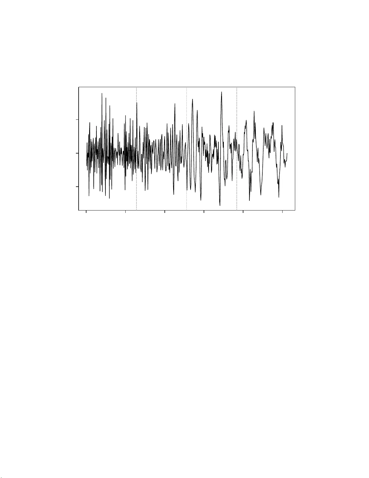
A note on state space represen tations of lo cally stationary w a v elet time series K. T rian taf yllop oulos ∗ G.P . Nason † No v ember 23, 2018 Abstract In this note w e show that the loc a lly stationary w avelet pro cess can be decomp osed int o a sum o f signals , each of which follo wing a moving average p r o cess with time-v ar ying parameters . W e then sho w that such moving average pro cesses are equiv alent to state space mo dels with stochastic design compo nents. Using a simple s imu la tion step, we prop ose a heur istic metho d of estimating the ab ov e state s pa ce mo dels a nd then we apply the methodolo gy to foreig n exchange ra tes da ta . Some key wor ds: wa velets, Haa r, lo c a lly stationary pr o cess, time series, state space, Kalman filter. 1 In tro d uction Nason et al. (2000 ) defin e a class of lo ca lly stationary time series making use of non-d ecimated w av elets. Let { y t } b e a sca lar time series, whic h is assumed to b e locally stationary , or stationary ov er ceratin in terv als of time (regimes), but o ve r all non -stationary . F or more details on lo ca l stationarit y the reader is r eferred to Dahlhaus (1997), Nason et el. (20 00), F rancq and Z ak oan (2001), and Mercurio and Sp oko iny (200 4). F or example, Figure 1 sho ws the nonstationary pro cess considered in Nason et al. (2000), whic h is the concatenation of 4 statio n ary moving a v erage pro cesses, bu t ea ch with differen t paramete r s. W e can see that within eac h of the four r egimes, the pro cess is w eakly stati onary , but o v erall the process is non-stationary . ∗ Department of Probability and S t atistics, Hicks Building, Unive rsity of S heffield, Sheffield S3 7RH, UK, email: k.t riantafyllopoulos@ sheffield.ac.uk † Department of Mathematics, Un iversi ty of Bristol, Bristol, U K 1 0 100 200 300 400 500 -2 0 2 time Concatenated process 0 100 200 300 400 500 -2 0 2 Figure 1: Concatenation of four MA time series with differen t parameters. Ov erall th e pro cess is n ot stationary . The dotted v ertical li n es indicat e the tr ansition b et we en one MA pro cess and th e next. The lo cally stationary w a ve let (LSW) p ro cess is a dou b ly indexed sto c hastic pro cess, defined by y t = − 1 X j = − J T − 1 X k =0 w j k ψ j,t − k ξ j k , (1) where ξ j k is a r andom o r thonormal incremen t sequence (b elow this will b e iid Gaussian) and { ψ j k } j,k is a d iscrete non-decimated family of wa v elets for j = − 1 , − 2 , . . . , − J , k = 0 , . . . , T − 1, based on a mother w a velet ψ ( t ) of compact su pp ort. Denote with I A ( x ) the indicator function, i.e. I A ( x ) = 1, if x ∈ A and I A = 0, otherwise. The simplest class of w av elets are the Haa r wa v elets, defin ed by ψ j k = 2 j / 2 I { 0 ,..., 2 − j − 1 − 1 } ( k ) − 2 j / 2 I { 2 − j − 1 ,..., 2 − j − 1 } ( k ) , for j ∈ {− 1 , − 2 , . . . , − J } and k ∈ { . . . , − 2 , − 1 , 0 , 1 , 2 , . . . } , wh ere j = − 1 is the finest scale. It is also assumed that E ( ξ j k ) = 0, for all j and k and so y t has zero mean. The orthonormalit y assumption of { ξ j k } implies that Cov( ξ j k , ξ ℓm ) = δ j ℓ δ k m , where δ j k denotes the Kr onec k er delta, i.e. δ j j = 1 and δ j k = 0, for j 6 = k . 2 The parameters w j k are the amplitudes of the LSW pro cess. Th e quan tit y w j k c haracter- izes the amount of eac h oscillation, ψ j,t − k at eac h scale, j , a n d lo cation, k (modifi ed by the random amplitude, ξ j k ). F or example, a la r ge v al u e of w j k indicates that there is a c hance (dep endin g on ξ j k ) of an oscillat ion, ψ j,t − k , at time t . Nason et al. (2000) con trol the ev olu- tion of the statistical c haracteristic s of y t b y coupling w j k to a function W j ( z ) f or z ∈ (0 , 1) b y w j k = W j ( k /T ) + O ( T − 1 ). Then, the smo othn ess prop erties of W j ( z ) cont r ol the p ossible rate of change of w j k as a function of k , whic h consequ ently controls th e ev olution of the statistica l prop erties of y t . T he sm o other W j ( z ) is, as a function of z , the slo wer that y t can ev olv e. Ultimately , if W j ( z ) is a constan t function of z , then y t is w eakly stationary . The non-stationarit y in the ab ov e studies is b etter u ndersto o d as lo cal-stationarit y so that the w j k ’s are close to eac h other. T o elab orate on this, if w j k = w j (time in v arian t), th en y t w ould b e wea kly stationary . The attractiv eness of the LSW p ro cess, is its abilit y to consider time-c hanging w j k ’s. Nason et al. (20 00) defin e the evo lu tionary w a vel et sp ectrum (EWS) to b e S j ( z ) = | W j ( z ) | 2 and discu ss metho ds of estimation. F ryzlewicz et al. (200 3) and F ryzlewicz (2 005) mo dify the LSW pr o cess to foreca st log-returns of non-stationary time series. These authors analyze d aily FTSE 100 time series using th e LSW to olb o x. F ryzlewicz and Nason (2006 ) estimate the EWS by using a fast Haar-Fisz algorithm. V an Bellegem and v on Sac hs (2008) consider adaptive estimation for the EWS and p ermit ju mp discontin uities in the sp ectrum. In this pap er w e sho w that the pro cess y t can b e decomp osed in to a sum of signals, eac h of whic h follo ws a moving av erage pro ce s s with time-v arying parameters. W e deplo y a heu r istic approac h for the estimation of the ab o ve mo ving a verage pr o cess and an examp le, consisting of foreig n exc hange rates, illustrates the prop osed method ology . 2 Decomp osition at scale j The LS W pr o cess (1 ) can b e written as y t = − 1 X j = − J x j t , (2) where x j t = T − 1 X k =0 w j k ψ j,t − k ξ j k . (3) F or computational simplicit y and without loss in generalit y , we omit th e min us sign of the scales ( − J, . . . , − 1) so that the summ ation in equation (2) is done from j = 1 (scale − 1) un til j = J (scale − J ). 3 Using Haar wa vel ets, we can see that at scale 1, w e h av e from (3) that x 1 t = ψ 1 , 0 w 1 t ξ 1 t + ψ 1 , − 1 w 1 ,t − 1 ξ 1 ,t − 1 , since there are only 2 n on-zero wa vele t co efficien ts. Th en we can re-wr ite (3) as x 1 t = α (0) 1 t ξ 1 t + α (1) 1 t ξ 1 ,t − 1 , whic h is a mo ving a verag e pro cess of order one, with time-v arying parameters α (0) 1 t and α (1) 1 t . T his p ro cess can b e referred to as TVMA(1) pro cess. In a similar wa y , for any scale j = 1 , . . . , J , w e can wr ite x j t = ψ j, 0 w j t ξ j t + ψ j, − 1 w j,t − 1 ξ j,t − 1 + · · · + ψ j, − 2 j +1 w j,t − 2 j +1 ξ j,t − 2 j +1 so th at we obtain the TVMA(2 j − 1) p ro cess x j t = α (0) j t ξ j t + a (1) j t ξ j,t − 1 + · · · + a (2 j − 1) j t ξ j,t − 2 j +1 , (4) where α ( ℓ ) j t = ψ j, − ℓ w j,t − ℓ , for all ℓ = 0 , 1 , . . . , 2 j − 1 and j = 1 , . . . , J . Th us the process y t is the sum of J TVMA pr o cesses. Ho wev er, w e note th at not all time-v arying paramet er s a ( ℓ ) j t ( ℓ = 0 , 1 , . . . , 2 j − 1) are indep endent, since, for a fixed j , they are all functions of the { w j t } series. W e adv o ca te that w j t is a signal and as s u c h we treat it as an unobserved sto c hastic pro cess. Ind eed, from the slo w ev olution of w j t , we can p ostulate that w j t − w j,t − 1 ≈ 0, whic h motiv ates a ran d om w alk evolutio n for w j t or w j t = w j,t − 1 + ζ j t , wher e ζ j t is a Gaussian white noise, i.e. ζ j t ∼ N (0 , σ 2 j ), f or σ 2 j a known v ariance, and ζ j t is indep endent of ζ k t , for all j 6 = k . The magnitude of the differences b et ween w j,t − 1 and w j t can b e cont r olled b y σ 2 j and this con trols on th e degree of ev olution of w j t as a function of t and hence on y t through (2). A t scale 1 w e can write x 1 t as x 1 t = ψ 1 , 0 w 1 t ξ 1 t + ψ 1 , − 1 w 1 ,t − 1 ξ 1 ,t − 1 = ( ψ 1 , 0 ξ 1 t + ψ 1 , − 1 ξ 1 ,t − 1 ) w 1 ,t − 1 + ψ 1 , 0 ζ 1 t ξ 1 t , where we hav e used w 1 t = w 1 ,t − 1 + ζ 1 t . Like wise at scale 2 w e ha v e x 2 t = ψ 2 , 0 w 2 t ξ 2 t + ψ 2 , − 1 w 2 ,t − 1 ξ 2 ,t − 1 + ψ 2 , − 2 w 2 ,t − 2 ξ 2 ,t − 2 + ψ 2 , − 3 w 2 ,t − 3 ξ 2 ,t − 3 = ( ψ 2 , 0 ξ 2 t + ψ 2 , − 1 ξ 2 ,t − 1 + ψ 2 , − 2 ξ 2 ,t − 2 + ψ 2 , − 3 ξ 2 ,t − 3 ) w 2 ,t − 3 + ψ 2 , 0 ζ 2 ,t − 2 ξ 2 t + ψ 2 , 0 ζ 2 ,t − 1 ξ 2 t + ψ 2 , 0 ζ 2 t ξ 2 t + ψ 2 , − 1 ζ 2 ,t − 2 ξ 2 ,t − 1 + ψ 2 , − 1 ζ 2 ,t − 1 ξ 2 ,t − 1 + ψ 2 , − 2 ζ 2 ,t − 2 ξ 2 ,t − 2 , where we ha ve used w 2 ,t − 2 = w 2 ,t − 3 + ζ 2 ,t − 2 , w 2 ,t − 1 = w 2 ,t − 3 + ζ 2 ,t − 2 + ζ 2 ,t − 1 and w 2 t = w 2 ,t − 3 + ζ 2 ,t − 2 + ζ 2 ,t − 1 + ζ 2 t . In general w e observ e that at an y scale j = 1 , . . . , J w e can write x j t = 2 j − 1 X k =0 ψ j, − k ξ j,t − k w j,t − 2 j +1 + 2 j − 2 X k =0 2 j − 2 X m = k ψ j, − k ξ j,t − k ζ j,t − m , t = 2 j , 2 j + 1 , . . . , (5) 4 where th e w j t ’s follo w the random walk w j,t − 2 j +1 = w j,t − 2 j + ζ j,t − 2 j +1 , ζ j,t − 2 j +1 ∼ N (0 , σ 2 j ) . (6) 3 A state space represen tation F or estimation p urp oses one could use a time-v arying moving av erage mo del in order to estimate { w j k } in (4). Mo ving a v erage pro cesses with time-v aryin g p arameters are useful mo dels for lo cally stati on ary time series data, but their estimation is more diffi cu lt that that of time-v arying au toregressive pro cesses (Hallin, 1986; Dahlh au s , 1997 ). The reason for this is that the time-dep endence of the mo ving a verag e co efficien ts may result in identifiabilit y problems. The consensus is that some restrictions of the parameter s pace of the time-v aryin g co efficien ts should b e applied; for more details t h e reader is referred to the ab o ve references as well as to T r ian tafyllop oulos and Naso n (2007). In this sect ion w e use a h euristic approac h for the estimation of the abov e models. First w e recast mo del (5)-(6) into state space form. T o end this we write x j t = A j t w j,t − 2 j +1 + ν j t , (7) where A j t = P 2 j − 1 k =0 ψ j, − k ξ j,t − k and ν j t = P 2 j − 2 k =0 P 2 j − 2 m = k ψ j, − k ξ j,t − k ζ j,t − m , for t = 2 j , 2 j + 1 , . . . . In ad d ition we assume that ξ i j t is indep endent of ζ i j s , for i = 1 , 2 and for an y t, s , so that ν j t ∼ N    0 , σ 2 j 2 j − 1 X k =0 ψ 2 j, − k (2 j − k − 1)    . (8) Equations (7), (6), (8) define a state space mo del for x j t and by d efining A t = ( A 1 t , . . . , A J t ) ′ and b y noting that ν j t is indep endent of ν k t , for an y j 6 = k , we obtain b y (2) a state space mo del f or y t , whic h essen tially is the sup erp osition of J state sp ace mo dels of the form of (7), (6), (8), eac h being a state space mo del for eac h scale j = 1 , . . . , J . Giv en a set of data y T = { y 1 , . . . , y T } , a heuristic w ay to estimate { w j t } , is to sim ulate in - dep end en tly all ξ j t from N (0 , 1), th u s to obtain sim u lated v alues f or A j t and then, conditional on A t , to app ly th e Kalman filter to the sta te space mo d el for y t . This pro cedure will giv e sim ulations from th e p osterior distributions of w j t and also from the predictiv e distributions of y t + h | y t . Th e estimator of w j t and the forecast of y t + h are conditional on the sim u lated v alues of { ξ j t } . F or comp eting sim u lated sequences { ξ j t } the p erform an ce of the ab ov e esti- mators/forecasts can b e judged b y comparing t h e resp ect ive lik eliho o d functions (whic h are easily calculable by the Kalman filter) or b y comparing th e resp ectiv e p ost er ior and forecast densities (by using sequent ial Ba yes factors). Another means of mo d el p erf ormance ma y be the co m putation of the mean square forecast error. 5 5.0e−06 1.0e−05 1.5e−05 1e−06 3e−06 5e−06 7e−06 0 100 200 300 400 500 Spectrum estimation for the GBP rate time scale 1 scale 2 Figure 2: Sim u lated v alues of p osterior estimate s of { S j t = w 2 j t } , for { y 1 t } (GBP rate). Sh o wn are s imulations of { S 1 t } and { S 2 t } , corresp onding to scales 1 and 2. W e illustrate this appr oac h by considering foreign exc h ange rates data. The data are collect ed in daily frequency from 3 January 2006 to and includ ing 31 Decem b er 2007 (consid- ering trading d a ys there are 5 01 observ ations). W e consider t wo exc h ange rates: US dollar with British p ound (GBP rate) and US dollar with Euro (EUR rate). After we transform the data to the log scale, we pr op ose to u s e the LSW pro cess in order to obtain estimates of the sp ectrum pro cess { S j t = w 2 j t } , for eac h sca le j . W e form th e v ector y t = ( y 1 t , y 2 t ) ′ , where y 1 t is the log-return v alue of GBP and y 2 t is the log-return v alue of EUR. F or eac h series { y 1 t } and { y 2 t } , resp ectiv ely , Figures 2 and 3 sho w sim u lations of the p osterior sp ectrum { S j t } , for scales 1 a n d 2. The smo othed estimates of these figures are ac h ieved by first computing the smo othed estimates u s ing the Kalman filter and then applyin g a standard Spline metho d (Green and Silv erman, 1994). W e note that, for the data set considered in this pap er, the estimates of Figures 2 and 3 are le s s smo oth than those prod uced by the metho d of Na son et al. (2000). Ho wev er, a higher degree of smoothness in our estimates ca n b e ac hiev ed by considering small v alues of the v ariance σ 2 j , whic h con trols the smoothness of the sho c ks in the random w alk of th e w ’s. 6 2.0e−06 6.0e−06 1.0e−05 1.4e−05 2.0e−06 6.0e−06 1.0e−05 1.4e−05 0 100 200 300 400 500 Spectrum estimation for the EUR rate time scale 1 scale 2 Figure 3: Sim u lated v alues of p osterior estimate s of { S j t = w 2 j t } , for { y 2 t } (EUR r ate). Sho wn are s imulations of { S 1 t } and { S 2 t } , corresp onding to scales 1 and 2. References [1] Anderson, P .L. and Meersc h aert, M.M. (200 5) Parame ter estimation for p erio d ically stationary time series. J ournal of Time Series Analysis , 26 , 489- 518. [2] Dahlhaus, R. (1997) Fitting time series mo dels to n onstationary pro ce ss es. Annals of Statistics , 25 , 1-37. [3] F rancq, C. and Zako an, J.M. (2001) Stationarit y of m ultiv ariate Marko v-sw itching ARMA mo dels. Journal of Ec onometrics , 102 , 339-364. [4] F ryzlewicz, P . (2005) Mod elling and forecasting fi nancial log-returns as lo ca lly stationary w av elet pr o cesses. Journal of Applie d Statistics , 32 , 503-5 28. [5] F ryzlewicz, P . and Nason, G.P . (2006) Haar-Fisz estimation of ev olutionary wa ve let sp ec- tra. J ournal of the R oyal Statistic al So ciety Se ries B , 68 , 611-63 4. 7 [6] F ryzlewicz, P ., V an Bellege m , S. and vo n Sachs, R. (2003) F orecasting non-stationary time series b y wa vele t pro ce ss mo delling. Annals of the Institute of Statistic al Mathema t- ics , 55 , 737- 764. [7] Green, P .J. and S ilv erman, B.W. (1994) Nonp ar ametric R e gr ession and Gener alize d Lin- e ar M o dels: A R oughness P enalty Appr o ach. C hapman and Hall. [8] Hallin, M. (1986) Nonstationary Q-dep endent pro cesses and time-v arying mo ving- a v erage mo d els - inv er tib ility prop ert y and the forecasting p roblem. A dvanc es in Applie d Pr ob ability , 18 , 170-210. [9] Mercurio, D. and Sp ok oin y , V. (200 4) S tatistical inference for time-inhomogeneous v olatilit y models. A nnals of Statistics , 32 , 57 7-602. [10] Nason, G.P ., vo n S achs, R. and K roisandt, G. (2000 ) W a ve let pro ce ss es and adaptiv e estimation of the ev olutionary w av elet s p ectrum. Journal of the R oyal Sta tistic al So ciety Series B , 62 , 271-29 2. [11] T rian tafyllop oulos, K. and Nason, G.P . (2007 ) A Ba ye s ian analysis of mo ving a v erage pro cesses with time-v arying parameters. Computational Statistics and Data Analy si s , 52 , 1025– 1046. [12] V an Bellege m , S. and von Sac hs, R. (2008) Lo ca lly adaptiv e estimation of evo lutionary w av elet sp ectra. Annal s of Statistics , (to app ear). 8