Controlled stratification for quantile estimation

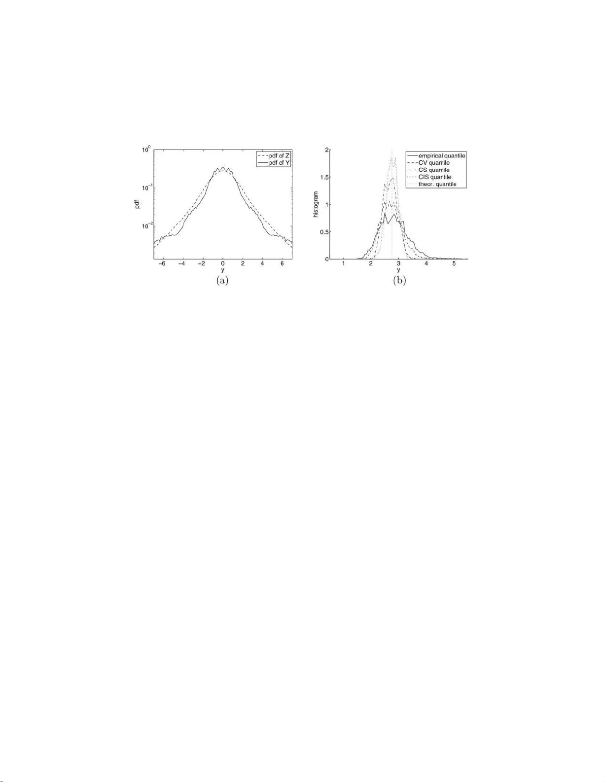
The Annals of Applie d Statistics 2008, V ol. 2, No. 4, 1554–1 580 DOI: 10.1214 /08-A OAS186 c  Institute of Mathematical Statistics , 2008 CONTR OLL ED STRA TIFICA TION F OR QUANTILE ESTIMA TION By Claire Cannamela, Jossel in Garnier and Ber trand Iooss Commissar iat ` a l’Ener gie Atomique, Universit ´ e P aris VII and Commissar iat ` a l’Ener gie Atomique In this pap er we propose and d iscuss v ariance redu ction tech- niques for t h e estimation of q uantil es of the output of a complex model with rand om input parameters. These techniques are b ased on the use of a reduced model, suc h as a metamod el or a response surface. The reduced mo d el can b e used as a con trol va riate; or a rejection metho d can b e implemented to sample the realiza tions of the input p arameters in prescrib ed relev ant strata; or the reduced model can b e used to determine a go o d biased distribution of the input parameters for the implemen tation of an imp ortance sampling strategy . The d ifferent strategies are analyzed and the asymptotic v ariances are computed, w hic h sho ws the benefit of an a daptive c on- trolled stra tification method. This method is finally applied to a real example (computation of the p eak cladding temp erature during a large-break loss of coolan t ac cident in a nuclear reactor). 1. In tro d u ction. Quan tile estimatio n is of fundamen tal imp ortance in statistic s as well as in practical applications [ La w and Kelton ( 1 991 )]. A main c h allenge in qu an tile estimation is that the n um b er of observ ations can b e limited. This is the case wh en the observ ations corresp ond to the output of exp ensive n umerical simulati ons. V ariance redu ction tec hn iqu es sp ecifi- cally designed for this problem hav e b een p rop osed and implemen ted. These tec hniques usually inv olv e imp ortance samp ling [ Glynn ( 1996 )], correlation- induction [ Avramidis and Wilson ( 1998 )] and con trol v ariates [ Hsu and Nelson ( 1987 ), Hesterb erg and Nelson ( 1998 )]. I n this pap er we fo cus our atten tion on v ariance reduction tec hniques based on the use of an auxiliary v ariable. F or the problem of the quan tile estimation of a computer co de output, the auxiliary v ariable is th e output of a reduced mod el, whic h is coarse bu t c heap from the compu tational time p oin t of view. W e will sho w ho w to u se Received F ebruary 2008; revised June 2008. Key wor ds and phr ases. Quantile estimation, Monte Carlo metho ds, v ariance reduc- tion, computer ex p erimen ts. This is an electronic r e print of the original article published by the Institute of Mathematical Statistics in The A nnals of Applie d Statistics , 2008, V ol. 2, No. 4 , 1554– 1580 . This reprint differs fro m the original in pag ina tion and t yp ographic detail. 1 2 C. CANN AMELA, J. GARNIER AND B. IOOSS it to fi nd conv enien t p arameters f or the stratified and imp ortance samp ling tec hniques [ Rubinstein ( 1981 )]. Quan tiles form a class of p erformance measures. Quan tile estimatio n for a real-v alued random v ariable (r.v.) Y aims at determining the lev el y such that the lik eliho o d that Y tak es a v alue lo wer than y is some prescrib ed v alue. W e assume that Y has an absolute ly con tin u ous cum ulativ e distribution function (cdf ) F ( y ) = P ( Y ≤ y ) and a con tinuously differen tiable probabilit y densit y (p df ) p ( y ). W e lo ok for an estimation of the α -quant ile y α defined b y F ( y α ) = α . In this p ap er we assu m e that Y = f ( X ) is the r eal-v alued output of a computer co de f that is CPU time exp ensiv e and w hose inpu t p arameters are random and mo deled b y the random vect or X ∈ R d with kno wn d istribu- tion. With th e adv ance of computing tec h nology and numerica l metho ds, the design, mo d eling and analysis of computer co de exp erimen ts ha ve b een the sub ject of int ense researc h dur ing the last t w o d ecades [ Sac ks et al. ( 1989 ), F ang, Li and Sudjianto ( 2006 )]. The problem of lo w or high quantil e esti- mation (smaller than 10% and larger than 90%) can b e r esolv ed by classical sampling tec hniques suc h as th e simp le Monte Carlo or Latin h yp ercub e tec hniques. These Mo n te Carlo metho d s can giv e imprecise qu an tile esti- mate (with large v ariance) if they are p erformed w ith a limited num b er of co d e runs, sa y , of the order of 200 [ Da vid ( 1981 )]. An alternativ e approac h is, to calculat e a tolerance limit r ather than a p ercen tile by using Wilk’s for- m u la [ Nutt and W all is ( 2004 )]. It p ro vides with a lo w num b er of co de runs , less than 200, sa y , a ma joring v alue of the desired p ercentil e with a giv en confidence lev el (e.g., 95% ). But th e v ariance of th is tolerance limit is larger than that of the emp irical estimate, for the same num b er of co de runs. Another w ell kn o wn app roac h for the uncertaint y analysis of complicate d computer mo dels consists in replacing the complex computer co d e b y a re- duced mo del, called metamo del or resp on s e su r face [ F ang, L i and Su djian to ( 2006 )]. Ho w ever, a lo w or high quantile estimate from a metamod el tends to b e substan tially differen t from the full computer mo del quant ile b ecause the metamo del is usually constructed b y smo othing of the computer mo del output. Recen tly , some authors ha v e tak en adv an tage of one particular t yp e of m etamodel: the Gaussian pro cess mo del [ Sac ks et al. ( 1989 )], whic h giv es not only a predictor (the mean) of a computer exp erimen t b ut also a lo cal in - dicator of pr ediction accuracy (the v ariance). In this con text, Oakley ( 2004 ), V azquez and Piera Martinez ( 2008 ) and Ranjan, Bingham and Mic hailidis ( 2008 ) hav e dev elop ed sequ ential p r o cedures to choose design p oints and to construct an accurate Gaussian pro cess metamo del, sp ecially near the re- gions of in terest, wh ere the qu an tile lies. Rutherford ( 2006 ) p rop oses to us e geostat istical conditional sim ulation tec hniques to obtain many r ealizations of the Gaussian p ro cess, whic h in tur n can giv e a quantile estimate. Ho w- ev er, all these tec hn iqu es are based on the construction of a Gaussian pro- cess mo d el whic h can b e difficult, alb eit p ossible [ Jones, Schonlau and W elc h CONTROLLED STRA TIFICA TION FOR Q U ANTILE ESTIMA TIO N 3 ( 1998 ), Sc h onlau and W elc h ( 2005 ), Marrel et al. ( 2008 )], in the high-dimensional con text ( d > 10). Moreo v er, in ind ustrial practice, a meta- mo del ma y already b e av ailable th at comes f rom a previous study or fr om a simplified physical mo del. T his is the situation we ha v e in mind. W e do not concen trate our effort on the construction of a more accurate metamo del, but on th e use of a giv en r educed mo del. In our work w e deal with this situation in wh ic h a r educed mo del is a v ail- able, in the form of a metamo del f r , whic h is a coarse approxi mation of the computer mo del f . The qu alit y of the metamo del may not b e kno w n; the metamod el ma y b e a simplified version of the compu ter co de (a one- dimensional version for a thr ee-dimensional problem, a resp onse surface de- termined during another study , . . . ); its input v ariables may b e a subset of the inpu t v ariables for the computer co de f . T h e full computer mo del f is assumed to b e v ery computationally exp ensive , while the ev aluation of the metamod el f r and the generation of the inpu t r.v. X are assumed to b e v ery fast (essen tially f ree). Therefore, the fo cus of this pap er is on ho w to exploit the metamo del to obtain b etter con trol v ariates, stratificatio n or imp ortance sampling than could b e obtained without it. In the real example we addr ess in Section 5 (computatio n of the p eak cladding temp erature of the nuclea r fuel du r ing a large-break loss of co olan t acciden t in a nuclea r reactor), the CPU time f or eac h call of the fun ction f is 20 min utes, while the metamodel f r is a linear fun ction and the input r.v. X is a collection of d = 53 ind e- p endent real-v alued r.v. with n ormal and log-normal distributions. In this example, we also study the relev ance of us in g more complex and p ow erful metamod els, su c h as the p opular Gaussian pro cess m o del. The u sual practice of quan tile estimatio n is to construct an estimator of the cdf of Y first, then to deduce an estimator of the α -quanti le of Y . In absence of the con trol v ariate, the standard metho d is the f ollo wing one. The estimation is based on a n -sample ( Y 1 , . . . , Y n ), that is to say , a set of n indep end en t and identic ally distributed r.v. with the p df p ( y ) of Y . The empirical estimator (EE) of th e cdf of F is ˆ F EE ( y ) = 1 n n X i =1 1 Y i ≤ y , (1) whic h leads to the standard estimator of the α -quantil e ˆ Y EE ( α ) = inf { y , ˆ F EE ( y ) > α } = Y ( ⌈ αn ⌉ ) , (2) where ⌈ x ⌉ is the in teger ceiling of x and Y ( k ) is the k th order statisti cs. Refined v ersions of this result based on inte rp olation and smo othing metho d s can b e foun d in th e literature [ Dielman, Lowry and Pfaffen b erger ( 1994 )]. The empirical estimator ˆ Y EE ( α ) has a bias and a v ariance of order 1 /n 4 C. CANN AMELA, J. GARNIER AND B. IOOSS [ Da vid ( 1981 )]. Th e empirical estimator is asymptotically norm al, √ n ( ˆ Y EE ( α ) − y α ) n →∞ − → N (0 , σ 2 EE ) , σ 2 EE = α (1 − α ) p 2 ( y α ) . (3) W e remark that the redu ced v ariance σ 2 EE is u s u ally larger w hen a larger quan tile is estimated (the p df at y α is then very small). The outline of the pap er is as f ollo ws. First we d escrib e quan tile estimation b y con trol v ariate in Sectio n 2 . Section 3 presen ts an origi nal controll ed stratificatio n method. Then, a con trolled imp ortance sampling strategy is analyzed in Section 4 . A r eal example is addressed in S ection 5 . 2. Quan tile estimation by Con trol V ariate (CV). In this section we presen t the w ell-known v ariance reduction tec hniques b ased on the use of Z = f r ( X ) as a con trol v ariate. Th e quanti les z α of Z are assumed to b e kno wn, as wel l as any exp ectation E [ g ( Z )] of a f u nction of Z . W e mean that these quantiti es can b e computed analytically , or they can b e estimated b y standard Mon te Carlo estimations with an arbitrary precision, since only the redu ced m o del f r is in v olved. 2.1. Estimation of the distribution function. A Control V ariate (CV) es- timator of F ( y ) with the real-v alued cont rol v ariate Z has the form ˆ F CV ( y ) = ˆ F EE ( y ) − C ( ˆ g n − E [ g ( Z )]) , (4) where the function g : R → R h as to b e c hosen by the us er [ Nelson ( 1990 )] and ˆ g n = 1 n P n i =1 g ( Z i ). The optimal parameter C is the correlation co efficien t b et w een g ( Z ) and 1 Y ≤ y whose v alue is unknown in practice. Therefore, the estimated parameter ˆ C is us ed instead. It is defined as the slop e estimator obtained from a least-squares regression of 1 Y j ≤ y on g ( Z i ): ˆ C = P n j =1 ( 1 Y j ≤ y − ˆ F EE ( y ))( g ( Z j ) − ˆ g n ) P n j =1 ( g ( Z j ) − ˆ g n ) 2 . As sh o wn by Hesterb erg ( 1993 ), the estimator ˆ F CV ( y ) with the estimated parameter ˆ C can b e rewritten as the weig h ted av erage ˆ F CV ( y ) = n X j =1 W j 1 Y j ≤ y (5) with W j = 1 n + ( ˆ g n − E [ g ( Z )])( ˆ g n − g ( Z j )) P n i =1 ( g ( Z i ) − ˆ g n ) 2 . CONTROLLED STRA TIFICA TION FOR Q U ANTILE ESTIMA TIO N 5 Note that P n j =1 W j = 1 . If g ( z ) = 1 z ≤ z α , then E [ g ( Z )] = α , ˆ g n = N 0 /n with N 0 = n X i =1 1 Z i ≤ z α and W j = α N 0 1 Z j ≤ z α + 1 − α n − N 0 1 Z j >z α . (6) As sho wn by Da vidson and MacKinnon ( 1992 ), the estimator ( 5 ) is equiv a- len t to the m aximum like liho o d estimator for probabilities. By usin g stan- dard results for the conv ergence of Monte C arlo estimators [ Nelson ( 1990 )], one fin ds √ n ( ˆ F CV ( y ) − F ( y )) n →∞ − → N (0 , σ 2 CV ) , (7) σ 2 CV = F ( y )(1 − F ( y ))(1 − ρ 2 I ) , where ρ I is the correlation co efficien t b et we en 1 Y ≤ y and 1 Z ≤ z α : ρ I = P ( Y ≤ y , Z ≤ z α ) − αF ( y ) p F ( y )(1 − F ( y )) √ α − α 2 . (8) This result can b e compared to the corresp onding cen tral limit theorem in absence of control , wh ic h claims that the emp irical estimator ˆ F EE defined b y ( 1 ) is asymptotically normal, √ n ( ˆ F EE ( y ) − F ( y )) n →∞ − → N (0 , σ 2 EE ) , σ 2 EE = F ( y )(1 − F ( y )) . Comparing with ( 7 ) r ev eals an asymptotic v ariance reduction of 1 − ρ 2 I . 2.2. Quantile estimation. Our goal is now to estimate the α -quanti le of Y b y using the CV estimator of the cdf of Y . W e consider the order statistic s ( Y (1) , . . . , Y ( n ) ) with the wei gh ts W ( i ) defined by ( 6 ) sorted according to the Y ( i ) . Using the estimator ( 5 ) of the cdf of Y , the C V estimator of the α - quan tile is ˆ Y CV ( α ) = Y ( K ) , K = in f ( j, j X i =1 W ( i ) > α ) . (9) Applying standard results for the v ariance reduction for Mo n te Carlo metho ds [ Da vid ( 1981 )], one finds that this estimator is asymptotically nor- mal with th e redu ced v ariance σ 2 CV , √ n ( ˆ Y CV ( α ) − y α ) n →∞ − → N (0 , σ 2 CV ) , σ 2 CV = α (1 − α ) p 2 ( y α ) (1 − ρ 2 I ) , (10) where p is the p df of Y and ρ I is the correlation coefficient b et wee n 1 Y ≤ y α and 1 Z ≤ z α : ρ I = P ( Y ≤ y α , Z ≤ z α ) − α 2 α − α 2 . 6 C. CANN AMELA, J. GARNIER AND B. IOOSS Comparing ( 10 ) w ith ( 3 ) r ev eals a v ariance r ed u ction b y the factor 1 − ρ 2 I . As exp ected, th e stronger Y and Z are correlate d, the larger the v ariance reduction is. It is not easy to build an estimator of the redu ced v ariance σ CV , b ecause this requires to estimate the p df p ( y α ). Ho w ev er, it is p ossible to b uild an estimator of the correlation coefficien t ρ I , whic h control s the v ariance redu ction. This estimator is the empir ical correlation co efficien t ˆ ρ I defined by ˆ ρ I = P n j =1 ( 1 Y j ≤ y − ˆ F EE ( y ))( 1 Z j ≤ z α − ˆ G n ( z α )) q P n j =1 ( 1 Y j ≤ y − ˆ F EE ( y )) 2 q P n j =1 ( 1 Z j ≤ z α − ˆ G n ( z α )) 2 | y = ˆ Y CV ( α ) (11) with ˆ G n ( z α ) = 1 n P n i =1 1 Z i ≤ z α . 2.3. The optimal CV e stimator . In the p revious section the con trol v ari- ate function is g ( z ) = 1 z ≤ z α , w hic h allo ws b oth an easy implemen tation and a substantia l v ariance reduction. In general, the v ariance reduction obtained with the CV estimator ( 4 ) d ep ends on the correlatio n coefficien t b et wee n 1 Y ≤ y and the con trol g ( Z ). Th e optimal control , which maximizes the cor- relation co efficien t, is obtained with the function [ Rao ( 1973 )] g ∗ ( z ) = P ( Y ≤ y | Z = z ) . (12) This f u nction is u sually un kn o wn , otherwise it could b e p ossible to compu te analytica lly th e cdf F ( y ) by taking the exp ectatio n of g ∗ ( Z ) , and solv e nu- merically the equation F ( y ) = α to get the qu an tile. Ho we v er, this result giv es the pr in ciple of refined CV metho ds using approximat ions of the op- timal con trol fu nction g ∗ . Cont in uous approxima tions hav e b een prop osed, that are ho wev er difficult to imp lement in p ractice [ Hastie and Tibshirani ( 1990 )]. Discrete app r o ximations ha ve b een presente d, w hic h h a ve b een sho w n to b e v ery efficient and easy to implement. W e no w describ e the dis- crete metho d prop osed by Hesterb erg and Nelson ( 1998 ). Let us choose m + 1 cutp oin ts 0 = α 0 < α 1 < · · · < α m = 1, and denote b y −∞ = z α 0 < z α 1 < · · · < z α m = ∞ the corresp onding quant iles of Z . The inte rv als ( z α j − 1 , z α j ] will b e used as strata to construct a stepwise constan t app r o ximation of the optimal cont rol. This construction is b ased on the str aight forw ard exp an s ion of the cdf of Y : F ( y ) = m X j =1 P j ( y )( α j − α j − 1 ) , (13) where P j ( y ) is the conditional probabilit y P j ( y ) = P ( Y ≤ y | Z ∈ ( z α j − 1 , z α j ]) . (14) CONTROLLED STRA TIFICA TION FOR Q U ANTILE ESTIMA TIO N 7 The qu an tiles of Z are kno wn , so the estimation of F ( y ) is reduced to the es- timations of the conditional p robabilities. The Po ststratified Sampling (PS) estimator of F ( y ) is ˆ F PS ( y ) = m X j =1 ˆ P j ( y )( α j − α j − 1 ) , where ˆ P j ( y ) = P n i =1 1 Z i ∈ ( z α j − 1 ,z α j ] 1 Y i ≤ y P n i =1 1 Z i ∈ ( z α j − 1 ,z α j ] . The P S estimator can b e written as a w eigh ted a v erage of 1 Y j ≤ y as well . It can also b e int erpreted as a CV estimator with g j ( Z ) = 1 Z ≤ z α j , j = 1 , . . . , m , as cont rol v ariates. Its v ariance is V ar ( ˆ F PS ( y )) = 1 n m X j =1 ( α j − α j − 1 )[ P j ( y ) − P 2 j ( y )] + O  1 n 2  . (15) Using Gaussian examples, Hesterb erg and Nelson ( 1998 ) ha ve shown that the optimal v ariance reduction (the one ac hiev ed with g ∗ ) can b e almost ac hiev ed with the discrete app ro ximation w ith t wo or three strata. Based on n umerical simulat ions, the authors recommend to choose the cutp oint α 1 = α for the PS strategy with t wo strata. They also apply the strategy w ith three strata on some particular examples. In the next section we will sho w that w e can go b ey ond the v ariance redu ction obtained with the optimal con trol g ∗ ( Z ) or its approxima tions by u sing the r educed mo del in a differen t wa y . 3. Quan tile estimation by Con trolled Stratification (CS). The use of a reduced mo d el to estimate d irectly the quantil es may b e not efficien t. Ind eed, as ment ioned in the in tro duction, the redu ced m o del is usu ally a metamo del or a resp on s e sur face that h as b een calibrated to mimic the resp onse of the complete mo del f ( X ) for t yp ical realizati ons of X , and not to pr edict the resp onse f ( X ) for exceptional realizatio ns of X . This is pr ecisely what is sough t wh en the purp ose is to estimate qu an tiles. Besides, it is v ery difficult to give an estimat e of the error w hen only the reduced model is used to estimate the quan tiles. In this section we exploit the existence of a redu ced mo d el Z = f r ( X ) in a differen t manner than the C V strategy . The idea of the previous section w as to use the reduced mo d el as a con trol v ariate, or equiv alen tly , p ost- stratificatio n, without mo difying the sampling. The idea of this section is to use it in ord er to imp lemen t nonpr op ortional stratified sampling in wh ic h w e do mo dify the sampling by rejection. The r ough idea is to generate many realizat ions of X , to ev aluate the corresp ond ing reduced resp onses f r ( X ) , 8 C. CANN AMELA, J. GARNIER AND B. IOOSS and to accept/rejec t the r ealizations dep ending on the resp onses f r ( X ) . The complete mo del f will b e used only with the accepted realizat ions. W e can therefore enforce the n umb ers of realizations of X such that f r ( X ) lie in prescrib ed inte rv als, and increase the n umbers of realizatio ns in the more imp ortan t interv als. 3.1. Estimation of the distribution function. Let u s c ho ose m + 1 cut- p oint s 0 = α 0 < α 1 < · · · < α m = 1 and denote by −∞ = z α 0 < z α 1 < · · · < z α m = ∞ the corresp onding quantil es of Z . As n oted in the previous sec- tion, the cdf of Y c an b e expanded as ( 13 ), so the estimation of F ( y ) is reduced to the estimatio ns of the conditional p robabilities P j ( y ) d efined by ( 14 ). Let us fi x a sequence of int egers N 1 , . . . , N m suc h that P m j =1 N j = n , where n is the total n umb er of sim ulations using the complete mo d el f . F or eac h j , w e use the rejection m etho d to samp le N j realizat ions of th e input r.v. ( X ( j ) i ) i =1 ,...,N j , such that the redu ced output r .v. Z ( j ) i = f r ( X ( j ) i ) lies in the in terv al ( z α j − 1 , z α j ]. F or eac h of these N j realizat ions, the out- put Y ( j ) i = f ( X ( j ) i ) is compu ted. Th e conditional probabilit y P j ( y ) can b e estimated by ˆ P j ( y ) = 1 N j N j X i =1 1 Y ( j ) i ≤ y , whic h giv es the CS estimator of F ( y ), ˆ F CS ( y ) = m X j =1 ˆ P j ( y )( α j − α j − 1 ) . (16) The estimator ˆ F CS ( y ) is unbiased and its v ariance is V ar ( ˆ F CS ( y )) = m X j =1 ( α j − α j − 1 ) 2 N j [ P j ( y ) − P 2 j ( y )] . (17) If th e num b er m of strata is fixed, if ( β j ) j =1 ,...,m is a sequence of p ositiv e r eal n um b ers such that P m j =1 β j = 1 , and if we choose N j = [ n β j ], where [ x ] is the int eger closest to x , then the estimator ˆ F CS ( y ) is asymptotically normal: √ n ( ˆ F CS ( y ) − F ( y )) n →∞ − → N (0 , σ 2 CS ) , (18) σ 2 CS = m X j =1 ( α j − α j − 1 ) 2 β j [ P j ( y ) − P 2 j ( y )] . W e firs t try to estimate the complete cdf F ( y ) f or all y ∈ R . CONTROLLED STRA TIFICA TION FOR Q U ANTILE ESTIMA TIO N 9 When Z is in dep endent of Y (wh ic h means that there is no control ), then w e hav e P j ( y ) = F ( y ) and V ar( ˆ F CS ( y )) = " m X j =1 ( α j − α j − 1 ) 2 N j # × [ F ( y ) − F ( y ) 2 ] . (19) If w e use a pr op ortional allocation in the strata β j = α j − α j − 1 , then N j = [( α j − α j − 1 ) n ] and we fi nd that the v ariance of the CS estimator is, m o dulo the round ing errors, equal to 1 n [ F ( y ) − F ( y ) 2 ], wh ic h is the v ariance of the empirical estimator. When the r.v. Z is an increasing function of Y (i.e. , to say , Z controls completely Y ), then w e obtain V ar ( ˆ F CS ( y )) = ( α j 0 − α j 0 − 1 ) 2 N j 0 [ p j 0 ( y ) − p j 0 ( y ) 2 ] ≤ ( α j 0 − α j 0 − 1 ) 2 4 N j 0 , where j 0 is su ch that y ∈ ( y α j 0 − 1 , y α j 0 ]. I f we choose equiprobable strata α j = j /m and prop ortional s amp ling β j = 1 /m , then V ar ( ˆ F CS ( y )) ≤ 1 / (4 mn ). The v ariance of the CS estimator h as therefore b een r ed u ced b y a factor of the order of 1 /m . Let us n o w lo ok for the estimation of the tail of cdf F ( y ) , in the region where F ( y ) ≃ 1 − δ with 0 < δ ≪ 1. If Z and Y ha v e p ositiv e correlation, then it is clear that we shou ld allo cate more simulati on p oin ts in the tail of the reduced mo del Z , so as to increase the num b er of r ealizations that are p oten tially relev an t. As an example, w e can c ho ose m = 4, α 1 = 1 / 2, α 2 = 1 − 2 δ , α 3 = 1 − δ , N j = n/ 4 for j = 1 , . . . , 4. Note that this partic ular c hoice allocates n/ 2 p oint s in the tail of the cdf of Z , wh ere z 1 − 2 δ < Z . If Z and Y are indep enden t, then equation ( 19 ) shows that this strat- egy in v olve s an in crease of the v ariance of the estimator by a factor 2: V ar ( ˆ F CS ( y )) ≃ 2 δ /n compared to the empirical esti mator V ar( ˆ F EE ( y )) ≃ δ /n . If Z and Y are so strongly correlated that the probabilit y of the joint ev ent Z ≤ z 1 − 2 δ and Y > y 1 − δ is neglig ible, then equation ( 19 ) sho ws that this strategy in v olve s a v ariance reduction by a factor sm aller than 2 δ : V ar ( ˆ F CS ( y )) ≤ 2 δ 2 /n . Th is means that the v ariance reduction can b e very sub stan tial in the case w here the v ariables Y and Z are correlated. 3.2. Quantile estimation. Here we consider the prob lem of the estima- tion of the α -quantile of Y , with α close to 1. F rom the pr evious results, we can pr op ose the estimator of the α -quan tile of Y giv en b y ˆ Y CS ( α ) = inf { y , ˆ F CS ( y ) > α } , 10 C. CANN AMELA, J. GARNIER AND B. IOOSS where ˆ F CS ( y ) is the CS estimator of the cdf of Y . Th e estimator ˆ Y CS ( α ) is asymptoticall y normal, √ n ( ˆ Y CS ( α ) − y α ) n →∞ − → N (0 , σ 2 CS ) , σ 2 CS = P m j =1 ( α j − α j − 1 ) 2 β j [ P j ( y α ) − P 2 j ( y α )] p 2 ( y α ) . If Z and Y are p ositiv ely correlated, then it is profitable to allocate more p oint s in the cdf tail of Z , so as to increase the num b er of p oten tially relev an t realizat ions. In the follo wing w e carry out n u merical sim u lations on a to y example in whic h n = 200 and α = 0 . 95. W e apply the CS metho d with m = 4 strata de- scrib ed here ab ov e ( α 1 = 0 . 5, α 2 = 0 . 9, α 3 = 0 . 95, N j = n/ 4 f or j = 1 , . . . , 4). W e u n derline that this example is very simp le and the reduced mo d el could certainly b e impro v ed. In particular, a Gaussian pro cess appr oac h w ould pro vide a very go o d appro ximation with a few tens of simulati ons (see Sec- tion 5 ). Th e redu ced mo del for th is to y example has in fact b een c hosen so as to ha v e approximat ely th e same qualit y (in terms of correlation co efficien ts ρ and ρ I ) as the one we exp ect in the case of the real example addr essed in Section 5 . Ou r fi rst ob jectiv e h ere is to v alidate the CS strategy on this to y example for w h ic h we can c h eck the CS estimations in terms of b ias and standard d eviation. O ur second ob jectiv e is to sho w that it can giv e go o d results with the parameters n = 200 and α = 0 . 95 even in the case in whic h ρ I is relativ ely small, which is the conte xt of the real example addressed in Section 5 . T oy example. 1D function. Let us consider the f ollo wing configuration. X is assumed to b e a Gaussian r.v. with mean zero and v ariance one. The functions f and f r are giv en by f r ( x ) = x 2 , f ( x ) = 0 . 95 x 2 [1 + 0 . 5 cos(10 x ) + 0 . 5 cos(20 x )] . (20) The quan tiles of Z = f r ( X ) are give n by z α = [Φ − 1 ((1 + α ) / 2)] 2 , wh ere Φ is the cdf of the N (0 , 1)-distribu tion. Th e quan tiles of Y are not kn o wn analyt- ically , as can b e seen in the plot of the p d f of Y in Figure 1 (a), obtained b y a series of 5 10 7 Mon te Carlo simulat ions. By using these Mon te Carlo sim- ulations, we ha v e ev aluated the theoretica l 0 . 95-quan tile of Y : y 0 . 95 = 3 . 66, and the correlation co efficien t b et ween Y and Z : ρ = 0 . 84. The efficiency of the CS metho d is related to the v alue of the ind icator correlation co efficien t ρ I , wh ic h can b e computed fr om the sim ulations and ( 11 ): ρ I = 0 . 62. W e compare the CS estimator with the empirical estimator and the CV esti- mator of the α -quanti le (Figure 1 (b)). One can observe that the quantile is p o orly predicted b y the empirical estimator, sligh tly b ette r p redicted by the CV estimator, while the CS estimator seems more efficien t. CONTROLLED STRA TIFICA TION FOR Q U ANTILE ESTIMA TIO N 11 Fig. 1. ( a ): Pdf of Y = f ( X ) and Z = f r ( X ) for X ∼ N (0 , 1) , obtaine d with 510 7 Monte Carlo simulations. ( b ): Estimation of the α -quantile of the r.v. Y = f ( X ) fr om a n -sample, with α = 95% and n = 200 . The thr e e histo gr ams ar e obtaine d fr om thr e e series of 10 4 ex- p eriments. The the or etic al quantile i s y α = 3 . 66 . The me an of the 10 4 empiric al estimations is 3 . 86 and their standar d deviation i s 0 . 83 . The me an of the 10 4 CV estimations is 3 . 74 and their standar d deviation is 0 . 744 . The me an of the 10 4 CS estimations i s 3 . 63 and their standar d deviation i s 0 . 381 . 3.3. A daptive c ontr ol le d str atific ation (ACS). W e first sho w that there exists an optimal c hoice for the allocation of th e simulat ion p oints in the strata. Let us consider th e CS estimation of the cdf of Y as describ ed in Section 3.1 . Let us fix y ∈ R . Th e CS estimator ( 16 ) of F ( y ) is asymp totica lly normal and its r educed v ariance σ 2 CS is giv en by ( 18 ). In fact, if the rounding errors are neglected, σ 2 CS /n is the v ariance of the C S estimator ˆ F CS ( y ) for an y n by ( 17 ). W e note that, if we c ho ose to allocate the sim ulation p oints prop ortionally in the strata, that is, w e c ho ose β j = α j − α j − 1 , then the redu ced v ariance of the CS estimator is equiv alen t to the redu ced v ariance of the PS estimator ( 15 ). T he imp ortant p oin t is that this prop ortional allocation is not efficien t, as we n o w sho w . If the num b er m of strata is fixed, as w ell as the cutp oin ts ( α j ) j =0 ,...,m and the total num b er n of simulatio ns, then it is p ossible to c ho ose the num b ers of sim ulations [ β j n ] p er stratum so as to minimize the v ariance of the C S esti- mator. It is well kn o wn that an optimal allocation p olicy for standard strati- fication exists [ Fishman ( 1996 ), Glasserman, Heidelb erger and Shahabud din ( 1998 )]. Here w e sho w th at an optimal allo cation p olicy exists for CS , in whic h the strata are d etermined by the metamodel. By denoting q j = ( α j − α j − 1 ) 2 [ P j ( y ) − P 2 j ( y )], the minimization p roblem arg min β ( m X j =1 q j β j ) , with the constrain ts β j ≥ 0 , m X j =1 β j = 1 12 C. CANN AMELA, J. GARNIER AND B. IOOSS has the unique solution β ∗ j = q 1 / 2 j P m l =1 q 1 / 2 l , j = 1 , . . . , m. With this optimal c hoice the reduced v ariance of the CS estimator ˆ F CS ( y ) is σ 2 OCS = ( m X j =1 ( α j − α j − 1 )[ P j ( y ) − P 2 j ( y )] 1 / 2 ) 2 . (21) Note that the optimal allo cation β ∗ j dep ends on y in general, whic h means that it is n ot p ossible to pr op ose an allo cation that is optimal for the esti- mation of the whole cdf of Y . Ho w ever, we can observ e the follo wing: (1) If the control is wea k, then P j ( y ) dep ends weakly on y , and the opti- mal allo cation is then β ∗ j = α j − α j − 1 . (2) If the con trol is strong, then we should allo cate more simulatio ns in the strata ( z α j − 1 , z α j ] around F ( y ). F or instance, let us assume a v ery strong con trol, in the sense that Z = ψ ( Y ) is an in creasing function of Y . Then P j ( y ) = P ( Y ≤ y | Z ∈ ( z α j − 1 , z α j ]) = P ( Y ≤ y | Y ∈ ( ψ − 1 ( z α j − 1 ) , ψ − 1 ( z α j )]) is equal to 1 if z α j ≤ ψ ( y ) [i.e., α j ≤ F ( y )] and to 0 if z α j − 1 > ψ ( y ) [i.e., α j − 1 > F ( y )]. In these t wo cases, q j and the optimal β ∗ j are zero, and all sim ulations should b e allocated in the stratum ( z α j 0 − 1 , z α j 0 ], for which α j 0 − 1 < F ( y ) ≤ α j 0 . Of course, the v ery strong con trol assumed here is not realistic, but th is example clearly illustrates the optimal allocation of simu- lations in the differen t strata. W e no w kno w that there exists an optimal allocation of the n s imula- tions in the m strata. This allo cation dep ends on the P j ( y ), whic h are the quan tities that we w an t to estimate. W e can therefore prop ose an adap tive pro cedure: (1) First apply the CS metho d with e n = n γ sim u lations, γ ∈ (0 , 1), and an a priori c hoice of the β j . W e then obtain a fi rst estimation of the conditional probabilities P j ( y ): e P j ( y ) = 1 [ β j e n ] [ β j e n ] X i =1 1 Y ( j ) i ≤ y . (2) Estimate the optimal allocation β ∗ j b y e β j = ( α j − α j − 1 )[ e P j ( y ) − e P j ( y ) 2 ] 1 / 2 P m l =1 ( α l − α l − 1 )[ e P l ( y ) − e P l ( y ) 2 ] 1 / 2 . CONTROLLED STRA TIFICA TION FOR Q U ANTILE ESTIMA TIO N 13 (3) Carry out the n − e n last simulatio ns b y allocating the s im u lations in eac h stratum in order to ac hieve the estimated optimal n um b er [ n e β j ] for all j . (4) Estimate P j ( y ) and F ( y ) b y ˆ P j ( y ) = 1 [ e β j n ] [ e β j n ] X i =1 1 Y ( j ) i ≤ y , ˆ F ACS ( y ) = m X j =1 ˆ P j ( y )( α j − α j − 1 ) . The A CS estimato r is un b iased conditionally on e β j > 0 for the j ’s suc h that β ∗ j > 0. The probabilit y of the complemen tary even t is of the order of exp( − c ˜ n ) w h ic h can b e usually neglected. The ACS estimator ˆ F ACS ( y ) is asymptoticall y normal, √ n ( ˆ F ACS ( y ) − F ( y )) n →∞ − → N (0 , σ 2 ACS ) , (22) σ 2 ACS = ( m X j =1 ( α j − α j − 1 )[ P j ( y ) − P 2 j ( y )] 1 / 2 ) 2 . The expression of the redu ced v ariance σ 2 ACS is the same as ( 21 ), wh ich is the one of the CS estimator with the optimal allo cation β ∗ j . The difference is that the v ariance σ 2 ACS /n is only r eac hed asymptotically as n → ∞ in the case of the A C S estimator, wh ile the v ariance is σ 2 OCS /n for all n in the case of the CS estimator with the optimal allocation. Note that the con v ergence of the A CS estimator is ensu red whatev er th e c hoice of the p ositiv e a priori n um b ers β j . In p ractice, a go o d a priori c hoice will sp eed up the con v ergence. W e now presen t an asymptotic analysis of the v ariance reduction for the CV, PS , CS and ACS m etho ds in the case of m = 2 str ata. In the PS metho d , or in the C S m etho d if we c ho ose the prop ortional allocation β j = α j − α j − 1 , the r ed u ced v ariance in ( 18 ) is σ 2 PS = F ( y )(1 − F ( y ))[1 − ρ 2 I ] , (23) where ρ I is the correlation co efficient b etw een 1 Y ≤ y and 1 Z ≤ z α defined by ( 8 ). σ 2 PS is also the reduced v ariance of the CV estima tor ( 7 ). Hesterb erg and Nelson ( 1998 ) ha v e already noticed that th e PS and CV es- timators are equiv alent. In the A CS metho d, the expression of the r educed v ariance σ 2 ACS in ( 22 ) is σ 2 ACS = F ( y )(1 − F ( y )) K 2 , K = α  1 + ρ I  (1 − α )(1 − F ( y )) αF ( y )  1 / 2  1 / 2  1 − ρ I  (1 − α ) F ( y ) α (1 − F ( y ))  1 / 2  1 / 2 + (1 − α )  1 + ρ I  αF ( y ) (1 − α )(1 − F ( y ))  1 / 2  1 / 2 14 C. CANN AMELA, J. GARNIER AND B. IOOSS ×  1 − ρ I  α (1 − F ( y )) (1 − α ) F ( y )  1 / 2  1 / 2 . If we assume th at the correlat ion coefficien t ρ I is small, then w e ge t the follo wing expansion with resp ect to ρ I : σ 2 ACS = F ( y )(1 − F ( y ))  1 − ρ 2 I 8 F ( y )(1 − F ( y )) + O ( ρ 3 I )  . (24) These r esults sh ow that the CV, PS , CS and A CS metho ds inv olv e a v ariance reduction of the same order wh en the goal is to estimate the cdf around the median F ( y ) ∼ 1 / 2. Ho wev er, when the goal is to estimate the cdf tail F ( y ) ∼ 0 or 1, the A CS metho d giv es a larger v ariance reduction. Of course, the CS metho d with a nearly optimal allo cation p olicy giv es th e same p erformance as the ACS metho d, b ut the implement ation of this metho d requires some a priori information on the correlation b et ween Y and Z to guess the correct allocation, while the A C S metho d finds it. The expressions that we hav e jus t deriv ed also give ind icatio ns for the c hoice of th e cutp oin t α . Indeed, the v ariance r eduction is all the larger as the correlation coefficien t ρ I is larger. F or instance, if w e assu me that Z = ψ ( Y ) is an increasing fu nction of Y , whic h mo d els a very strong cont rol, then one finds ρ I =           α (1 − F ( y )) (1 − α ) F ( y )  1 / 2 , if z α < ψ ( y ),  (1 − α ) F ( y ) α (1 − F ( y ))  1 / 2 , if z α ≥ ψ ( y ). As a fu nction of α , this fun ction is maximal w hen α = F ( y ). Th is sho ws that, if the goal is to estimate the cdf of Y around some y , then it is inte resting to c ho ose α = F ( y ). W e can also revisit the asymptot ic analysis of the v ariance redu ction for the CV, PS, CS and A C S metho d s in the case of a large num b er m of strata. In the PS metho d and in the C S metho d w ith the prop ortional allocation β j = α j − α j − 1 , the r ed u ced v ariance is ( 18 ). If the conditional probabilit y P ( Y ≤ y | Z ) has a co n tin u ous densit y g ∗ with resp ect to the Leb esgue measure, then ( 18 ) is a Riemann sum that has the follo wing limit as m → ∞ : σ 2 PS = E [ P ( Y ≤ y | Z ) − P ( Y ≤ y | Z ) 2 ] = F ( y ) − E [ P ( Y ≤ y | Z ) 2 ] . This is actually the redu ced v ariance of the optima l CV esti mator, w h en the optimal contro l f u nction g ∗ defined b y ( 12 ) is used. In the A CS metho d, the expression of th e reduced v ariance σ 2 ACS is ( 22 ), wh ich has th e follo wing limit as m → ∞ : σ 2 ACS = E [( P ( Y ≤ y | Z ) − P ( Y ≤ y | Z ) 2 ) 1 / 2 ] 2 . CONTROLLED STRA TIFICA TION FOR Q U ANTILE ESTIMA TIO N 15 The Cauch y–Sc hw arz inequalit y clearly sho ws that the v ariance red u ction is larger for the A C S metho d than for the optimal CV metho d u s ing the optimal cont rol fu nction g ∗ . Whatev er the v alue of m ≥ 2, we can also use the Cauc h y–Sch wa rz in- equalit y to chec k that the redu ced v ariance for the PS metho d (or f or the CS metho d with the pr op ortional allocation) σ 2 PS = m X j =1 ( α j − α j − 1 )[ P j ( y ) − P 2 j ( y )] is alwa ys larger than the r educed v ariance ( 22 ) for the A CS metho d . Finally , it is relev an t to estimat e the additional computational cost of con trolled stratificati on compared to empirical estimation. I t is of the ord er of ( N r − n ) T X + N r T f r , where N r is the num b er of ev aluations of f r and X , T X is the compu tational time for the generation of a realization of the input r.v. X , and T f r is the computational time for the call of the function f r . F or the CS m etho d with the allocation β j , we hav e E [ N r ] = n m X j =1 β j α j − α j − 1 ≤ n min j ( α j − α j − 1 ) , where the last inequalit y holds uniformly in β . Besides, N r has fl uctuations of the order of √ n . The same estimate holds true for the ACS metho d. In the real example w e hav e in mind (in whic h the computational time for th e function f is 20 m inutes), this additional cost is negligible. 3.4. Quantile estimation by adaptive c ontr ol le d str atific ation. In this s ec- tion we u se the ACS strategy to estimate the α -quanti le of Y , with α close to 1 . W e prop ose the f ollo wing pro cedur e: (1) First apply the CS metho d with e n = n γ sim u lations, γ ∈ (0 , 1), and with an a p riori allocation p olicy β j , so that a first estimate of the conditional probabilities P j ( y ) can b e obtained: e P j ( y ) = 1 [ β j e n ] [ β j e n ] X i =1 1 Y ( j ) i ≤ y . The corresp ond ing estimators of the cdf and the α -quantile of Y are e F ( y ) = m X j =1 ( α j − α j − 1 ) e P j ( y ) , e Y α = inf { y , e F ( y ) > α } . (2) Estimate the optimal allo cation β ∗ j for th e estimated α -quan tile e Y α b y e β j = ( α j − α j − 1 )[ e P j ( e Y α ) − e P j ( e Y α ) 2 ] 1 / 2 P m l =1 ( α l − α l − 1 )[ e P l ( e Y α ) − e P l ( e Y α ) 2 ] 1 / 2 . (25) 16 C. CANN AMELA, J. GARNIER AND B. IOOSS (3) Carry out the n − e n fin al sim u lations b y allo cating the simulatio ns in eac h stratum in order to ac hiev e the estimated optimal n umber [ e β j n ]. (4) Estimate P j ( y ) and F ( y ) b y ˆ P j ( y ) = 1 [ e β j n ] [ e β j n ] X i =1 1 Y ( j ) i ≤ y , ˆ F ACS ( y ) = m X j =1 ˆ P j ( y )( α j − α j − 1 ) . The A CS estimator of the α -quantil e y α is ˆ Y ACS ( α ) = inf { y , ˆ F ACS ( y ) > α } . The estimator ˆ Y ACS ( α ) is asymptotically normal, √ n ( ˆ Y ACS ( α ) − y α ) n →∞ − → N (0 , σ 2 ACS ) , σ 2 ACS = { P m j =1 ( α j − α j − 1 )[ P j ( y α ) − P 2 j ( y α )] 1 / 2 } 2 p 2 ( y α ) . T o summarize, we ha v e found the follo w in g expressions of the reduced v ariance for the differen t metho ds: • for the emp irical estimator, σ 2 EE = α (1 − α ) p 2 ( y α ) . • for the PS estimator or for the CV estimator with the prop ortional allo- cation β j = α j − α j − 1 [see ( 10 )], σ 2 PS = α (1 − α ) p 2 ( y α ) × (1 − ρ 2 I ) . • for the ACS estimator with t wo strata separated b y α σ 2 ACS = α (1 − α ) p 2 ( y α ) ×  1 − ρ 2 I 8 α (1 − α ) + O ( ρ 3 I )  . Here ρ I is the correlation co efficient b et wee n 1 Y ≤ y α and 1 Z ≤ z α giv en by ( 11 ). This sh o ws that the C V, PS , CS and A CS metho ds giv e v ariance reductions of th e same ord er when th e goal is to estimate quan tiles close to the median α ∼ 1 / 2. How ev er, when the goal is to estimate large quantile s α ∼ 0 or 1, the ACS metho d is muc h more efficien t. 3.5. Simulations. W e no w present a series of numerica l simulatio ns that illustrate the theoret ical r esu lts presen ted in this pap er. These examples are simple and they are used to v alidate the A C S metho d wh en n = 200, α = 0 . 95 and th e reduced mo del has p o or qu alit y (i.e., ρ I is small). W e will address in Section 5 a real example in whic h these conditions h old. CONTROLLED STRA TIFICA TION FOR Q U ANTILE ESTIMA TIO N 17 T oy example. 1D function. Let us revisit th e to y example based on the 1D fu nction ( 20 ) and lo ok for the α -quan tile of Y with α = 95%. W e compare the p erformances of the empirical estimator ( 2 ), the C V estimator ( 9 ) with the con trol v ariate Z , and the ACS estimator. The A CS metho d is first implemen ted with tw o strata [0 , α 1 ] and ( α 1 , 1] with the cutp oin t α 1 = α . W e use ˜ n = 2 n/ 10 simulatio ns for the estimation ( 25 ) of the optimal allo cation, with n/ 10 sim ulations in eac h stratum. The results extracted from a series of 10000 simulati ons are su mmarized in T able 1 . Note that the A CS metho d allocates 85% of the s imulatio ns in the stratum [0 , 0 . 95], and 15% in the stratum (0 . 95 , 1]. Th is sho ws that we deal with a configur ation wh ere the n um b er of simulat ions in the stratum (0 . 95 , 1] has to b e increased compared to the exp ected v alue in the case wh ere there is no con trol, wh ere only 5% of the simulatio ns should b e allocated in the stratum (0 . 95 , 1]. W e ha v e also imp lemented th e A CS metho d w ith 3 strata [0 , α 1 ], ( α 1 , α 2 ], ( α 2 , 1], with cutp oint s α 1 = 0 . 85 and α 2 = 0 . 95. W e u s e 3 n/ 10 sim u lations for the ev aluation ( 25 ) of the optimal allo cation, with n / 10 simulati ons in eac h of the thr ee strata. Th e results extracted fr om a series of 10000 simulatio ns are presen ted in T able 1 . T he v ariance reduction for the A C S metho d with three strata is v ery imp ortan t. T he standard d eviation of the A CS estimator is 3 times smaller compared to the emp irical estimator of the CV estimator. Note that the optimal allo cation should attribute a fraction β 1 < 0 . 1 to the first stratum, but the n umber 0 . 1 cannot b e lo wered du e to the fact that n/ 10 simula tions in the first stratum [0 , α 1 ] were already used in the firs t step of the estimation. The previous simulati ons w ere carried out with the sample size n = 2000. In such a case, the A CS metho d is robust, in the sense that the choi ce of the n um b er ˜ n of sim ulations dev oted to the estimatio n of the optimal allocation is not critical. When n is smaller, suc h as n = 200, then the c hoice of ˜ n b e- comes critical: if ˜ n is to o s mall, then the estimatio n of the optimal allocation T able 1 Estimation of the α -quantile with α = 0 . 95 , n = 2000 , y α = 3 . 66 Metho d Quantit y Mean Standard deviation Empirical estimation ˆ Y EE ( α ) 3.66 0.33 CV estimation ˆ Y CV ( α ) 3 . 65 0 . 29 ACS metho d with 2 strata e β 1 0 . 86 0 . 02 [0 , 0 . 95], (0 . 95 , 1] ˆ Y ACS ( α ) 3 . 65 0 . 28 ACS metho d with 3 strata e β 1 0 . 10 0 . 02 [0 , 0 . 85], (0 . 85 , 0 . 95], (0 . 95 , 1] e β 2 0 . 58 0 . 02 e β 3 0 . 32 0 . 01 ˆ Y ACS ( α ) 3 . 65 0 . 12 18 C. CANN AMELA, J. GARNIER AND B. IOOSS T able 2 Estimation of the α -quantile with α = 0 . 95 , n = 200 , y α = 3 . 66 Metho d Quantit y Mean Standard deviation Empirical estimation ˆ Y EE ( α ) 3.88 0.83 CV estimation ˆ Y CV ( α ) 3.73 0.74 ACS metho d with 3 strata e β 1 0.14 0.16 [0 , 0 . 85], (0 . 85 , 0 . 95], (0 . 95 , 1] e β 2 0.55 0.11 e β 3 0.31 0.06 ˆ Y ACS ( α ) 3.62 0.38 ma y fail during the first step of the ACS metho d; if ˜ n is to o large, then n − ˜ n ma y b e to o small and it ma y b e imp ossible to allo cate th e estimated optimal n um b er of s imulatio ns to eac h stratum du r ing the second step of the ACS metho d. W e ha ve applied the A CS method with n = 200 to the example 1, and it turns out that the ACS metho d with ˜ n = n/ 10 is still efficie n t. Ho wev er, w e cannot claim that this will b e the case for all applicatio ns. The resu lts obtained from a series of 10000 s imulatio ns are summarized in T able 2 . T he standard deviations of the estimations of the β j ’s are muc h larger than in the case n = 2000, b ut the qualit y of the estimation of the optimal allocation is just go o d enough to allo w for a significa n t v ariance reduction for the qu an tile estimation. The standard deviation of the A C S estimator is here 2 times smaller compared to the empirical estimator or the CV estimator. I f n = 100, then the ACS metho d fails (in the sense that some sim ulations giv e ˜ β 1 = 0 ), and the CS metho d w ith an allo cation of the sim u lation p oin ts prescrib ed by the user should b e c hosen. 4. Quan tile estimation with Cont rolled Imp ortance S am p ling (CIS). W e consider the s ame p roblem as in the previous sections. In this section we sho w that the reduced mo d el can b e u sed to help design a biased distri- bution of the inpu t r.v. X in order to imp lemen t an efficient imp ortance sampling (IS ) strategy . The standard IS metho d consists in simulating the n -sample of the r.v. X according to a biased distribution, and to m u ltiply the output by a lik eliho o d ratio to reco v er an unbiased estimator. In the case in w h ic h the biased distribu tion fav ors th e o ccurrence of the even t of imp ortance, the v ariance of the estimator can b e dr astically redu ced com- pared to the standard empirical Mon te Carlo estimator. Adaptiv e v ersions of the IS pro cedur e ha v e b een prop osed and studied, whose principle is to estimate first a “goo d ” biased distribution that is to sa y , a d istrib ution that prop erly fa vors the o ccurrence of the even t of imp ortance, b efore using this biased distribution as in the standard IS estimatio n. W e will pr op ose an estimator of the cdf of Y first, then an estimator of the α -quan tile of Y , by CONTROLLED STRA TIFICA TION FOR Q U ANTILE ESTIMA TIO N 19 a con trolled imp ortance sampling (CIS) pro cedure. In this pro cedu re, the reduced mo del f r and the asso ciated r.v. Z = f r ( X ) are u sed to determine the biased distribution, while the complete mo del f is u s ed to p erform the estimatio n. 4.1. Estimation of the distribution function. An IS estimator of the cdf of Y = f ( X ) is ˆ F IS ( y ) = 1 n n X i =1 1 f ( X i ) ≤ y q ori ( X i ) q ( X i ) , X i ∼ q , (26) where q ori is the original p df of X and q is the biased p df c hosen by the user. In pr actice , it can b e usefu l to use a v ariant in whic h the denominator n in ( 26 ) is replaced by P n i =1 q ori ( X i ) /q ( X i ), in order to enforce ˆ F IS ( y ) → 1 as y → ∞ . Other alternativ es can b e f ou n d in Hesterb erg ( 1995 ). The estimator ˆ F IS ( y ) conv erges almost su rely to F ( y ) when n → ∞ . In fact, the estimator ˆ F IS ( y ) is unbiased as so on as the sup p ort of the original p df q ori is includ ed in the supp ort of the biased p df q . The v ariance of ( 26 ) is giv en by V ar[ ˆ F IS ( y )] = 1 n  Z 1 f ( x ) ≤ y q ori ( x ) 2 q ( x ) dx − F ( y ) 2  . (27) The IS can in v olve a dramatic v ariance reduction compared to the standard empirical estimator if the biased p d f q is prop erly c hosen. The v ariance of ˆ F IS ( y ) is minimal [ Rubinstein ( 1981 )] wh en the biased p d f is tak en to b e equal to the optimal p df defined by q ∗ ( x ) = 1 f ( x ) ≤ y q ori ( x ) R 1 f ( x ′ ) ≤ y q ori ( x ′ ) dx ′ . (28) This result cannot b e d irectly used to p erform the simulati ons b ecause the normalizing constan t of the optimal p df is th e quant it y that is sought . How- ev er, this remark giv es the basis of an adaptiv e pro cedure where the optimal densit y is estimated. The parametric app roac h for the adaptiv e IS approac h is the follo wing one. W e first c ho ose a family of p d fs Q = { q γ ; γ ∈ Γ } and we then try to estimate the parameter γ . In this sect ion w e assume that the family of p dfs Q is parameterized b y the first t w o moment s: γ = ( λ, C ) : λ ∈ R d is the exp ectation and C ∈ M d ( R ) is the co v ariance matrix of X wh en the p df of X is q γ . The strategy to determine the b est biased d ensit y in the family Q is based on the follo wing remark. Th e theoretical optimal densit y is q ∗ and it is giv en by ( 28 ). The exp ectation and co v ariance matrix of the rand om v ector X u nder q ∗ are λ ∗ = R x 1 f ( x ) ≤ y q ori ( x ) dx R 1 f ( x ) ≤ y q ori ( x ) dx and C ∗ = R xx t 1 f ( x ) ≤ y q ori ( x ) dx R 1 f ( x ) ≤ y q ori ( x ) dx − λ ∗ λ ∗ t . (29) 20 C. CANN AMELA, J. GARNIER AND B. IOOSS The idea is to choose in the family Q the p df q γ whic h has exp ectati on λ ∗ and cov ariance matrix C ∗ , that is to sa y , we c h o ose th e p d f q γ ∗ with γ ∗ = ( λ ∗ , C ∗ ). The problem is no w reduced to the estimation of λ ∗ and C ∗ . If we assu me that th e reduced mo del is so c h eap that w e can use as man y sim ulations based on f r as desired, then w e can estimate λ ∗ and C ∗ b y            ˆ λ = P ˜ n i =1 X i 1 Z i ≤ y q ori ( X i ) /q 0 ( X i ) P ˜ n i =1 1 Z i ≤ y q ori ( X i ) /q 0 ( X i ) , ˆ C = P ˜ n i =1 X i X t i 1 Z i ≤ y q ori ( X i ) /q 0 ( X i ) P ˜ n i =1 1 Z i ≤ y q ori ( X i ) /q 0 ( X i ) − ˆ λ ˆ λ t , X i ∼ q 0 , (30) where q 0 is an a priori p df c h osen b y the user. If no a p riori information is a v ailable, then the c h oice q 0 = q ori is natural. The estimators ˆ λ and ˆ C are w ell defin ed on S ˜ n i =1 { Z i ≤ y } . F or completeness, we can set ˆ λ = 0 and ˆ C = I d on the complemen tary ev en t, wh ose p robabilit y is of the form exp( − c ˜ n ). As ˜ n → ∞ , the estimators ˆ λ and ˆ C con v erge almost surely to λ ∗ r = R x 1 f r ( x ) ≤ y q ori ( x ) dx R 1 f r ( x ) ≤ y q ori ( x ) dx and C ∗ r = R xx t 1 f r ( x ) ≤ y q ori ( x ) dx R 1 f r ( x ) ≤ y q ori ( x ) dx − λ ∗ r λ ∗ r t , whic h are close to λ ∗ and C ∗ if f r is a go o d enough red u ced mo d el. The v ariance of the CIS estimator of F ( y ) u sing the biased p df determined b y the metamod el is ( 27 ) with q = q γ ∗ r , γ ∗ r = ( λ ∗ r , C ∗ r ). ˆ F CIS is asymptotically normal, √ n ( ˆ F CIS ( y ) − F ( y )) n →∞ − → N (0 , σ 2 CIS ) , σ 2 CIS = Z 1 f ( x ) ≤ y q ori ( x ) 2 q γ ∗ r ( x ) dx − F ( y ) 2 . Note that the selected b iased p d f dep ends on y . Indeed, it is not p ossible to prop ose a b iased p df that is efficien t for all v alues of y . Th is is n ot s urprising, since the pr in ciple of the IS metho d is to fav or the r ealizat ions that prob e a sp ecific region of the state space that is imp ortan t for the target function whose exp ectatio n is sought (here, x 7→ 1 f ( x ) ≤ y ). 4.2. Quantile estimation. In this sub section we lo ok for the α -quanti le of Y . The CIS strategy consists in determining a b iased p df that is efficient for the estimatio n of th e exp ectatio n E [ 1 f r ( X ) ≤ z α ] = Z 1 f r ( x ) ≤ z α q ori ( x ) dx = α, (31) where f r is the reduced mo del and z α is the α -qu antile of Z , which is assum ed to b e known. Th e determination of a biased p df q that minimizes the IS CONTROLLED STRA TIFICA TION FOR Q U ANTILE ESTIMA TIO N 21 estimator of the quant it y ( 3 1 ) will giv e a p df that prob es the imp ortant regions for th e estimation of the α -quantile of Z , and also of th e α -quan tile of Y if the reduced mo del is correlated to th e complete computer mo del. As in the p revious subsection, we will lo ok for the biased p d f in a family Q of p dfs q γ parameterized by the first tw o momen ts γ = ( λ, C ) . By usin g only the reduced mo del, we estimate the parameter γ with the estimator ( 30 ) with y = z α . Next we apply the IS estimator ( 26 ) of the cdf of Y b y using the complete mo del and the biased densit y q ˆ γ , ˆ γ = ( ˆ λ, ˆ C ). Finally , the estimator of the α -quantile is ˆ Y CIS ( α ) = inf { y , ˆ F IS ( y ) > α } . It is asymp totically normal, √ n ( ˆ Y CIS ( α ) − y α ) n →∞ − → N (0 , σ 2 CIS ) , σ 2 CIS = 1 p 2 ( y α )  Z 1 f ( x ) ≤ y α q ori ( x ) 2 q γ ∗ r ( x ) dx − α 2  . In the case where the redu ced mo d el is not so c h eap, adaptiv e I S strategie s can b e used with the reduced m o del to estimate the parameters of the bi- ased densit y [ Oh and Berger ( 1992 )]: roughly sp eaking, at generation k , the parameter γ k is estimated by using a standard IS strategy us ing the biased p df γ k − 1 obtained du ring the computations of the previous generation. 4.3. Simulations. Let u s consider the case wh ere X = ( X 1 , X 2 ) is a ran- dom v ector with ind ep endent Gaussian entrie s with zero mean and v ariance one. The functions f and f r are giv en b y f r ( x ) = | x 1 | x 1 + x 2 , (32) f ( x ) = 0 . 95 | x 1 | x 1 [1 + 0 . 5 cos(10 x 1 ) + 0 . 5 cos(20 x 1 )] (33) + 0 . 7 x 2 [1 + 0 . 4 cos( x 2 ) + 0 . 3 cos(14 x 2 )] . The p df of Y = f ( X ) and Z = f r ( X ) are plotted in Figure 2 (a). By using Mon te Carlo sim ulations, we ha ve ev aluated the correlation co efficient b e- t ween Y and Z : ρ = 0 . 90. F r om ( 11 ), we ha v e also ev aluated the ind icator correlatio n co efficien t: ρ I = 0 . 64. The emp ir ical estimator and the CIS es- timator of the α -qu an tile of Y are compared in Figure 2 (b). The family Q consists of the set of t wo-dimensional Gaussian p dfs parameterized by their means and cov ariance matrices. The comparison is also made with the CV estimator and the C S estimator and it app ears that the v ariance of the CIS estimator is significan tly smaller than the one of the other estimators. CIS is the b est strategy in this example. Ho w ev er, CIS (in the pr esent v ersion) is successful only when one un ique imp ortan t region exists in the state space. F or in stance, in the case of the 1D fun ction treated in the p re- vious sections (where there are t w o equally imp ortan t regions far aw a y from eac h other due to the parit y of the function f ), the CIS strategy fails in the 22 C. CANN AMELA, J. GARNIER AND B. IOOSS Fig. 2. ( a ): Pdf of Y = f ( X 1 , X 2 ) and Z = f r ( X 1 , X 2 ) for X 1 , X 2 ∼ N (0 , 1) . ( b ): Es- timation of the α -quantile of Y fr om a n -sample, wi th α = 0 . 95 and n = 200 . The f our histo gr ams ar e obtaine d fr om f our series of 5000 exp eriments. The me an of the empiri c al estimations is 2 . 83 and their standar d deviation is 0 . 52 . The me an of the CV estimations is 2 . 74 and their standar d deviation i s 0 . 38 . The m e an of the CS estimations is 2 . 71 and their standar d deviation is 0 . 25 . The me an of the CI S estimations is 2 . 77 and their standar d deviation is 0 . 21 . The the or etic al quantile (obtaine d f r om a series of 5 10 7 simulations) is y α ≃ 2 . 75 . sense that the algorithm to determine the biased p df do es n ot conv erge. The use of mixed p df mo dels should b e considered to ov ercome this limitation and will b e the su b ject of f u rther researc h. 5. Application to a n uclear safet y problem. In this section w e apply the con trolled stratification an d con tr olled imp ortance sampling metho dologies on a complex computer mo del used for nuclear reactor safet y . It sim ulates a h yp othetic thermal-h ydraulic scenario: a large-break loss of co olan t accident for which the quantit y of in terest is the p eak cladding temp erature. Th is sce- nario is part of the Benc h mark for Un certain t y Analysis in Best-Estimate Mo deling for Design, Op eration and Safet y Analysis of Ligh t W ater Reac- tors [ P etruzzi et al. ( 2004 )] pr op osed by the Nuclear E nergy Agency of the Organisation for Economic Co-op eration and Dev elopmen t (OCDE/NEA). It has b een implemente d on the computer cod e Cathare of the Commissariat ` a l’Energie At omique (CEA). In this exercise the 0 . 95-quant ile of the p eak cladding temp erature has to b e estimated with less than 250 computations of the computer mod el. Th e CPU time is t wen t y min utes for eac h simu- lation. Th e complexit y of the computer mo del lies in the h igh-dimensional input space: 53 random input parameters (physical la ws essen tially , but also initial conditions, material p rop erties and geometrical mo d eling) are consid- ered, with n ormal and log-normal d istributions. This num b er is rather large for the metamodel construction pr oblem. CONTROLLED STRA TIFICA TION FOR Q U ANTILE ESTIMA TIO N 23 Scr e ening and line ar r e gr ession str ate gy. T o simplify the problem, we ap- ply first a screening tec h nique, based on a sup ersaturated design [ Lin ( 1993 )] with 30 n umerical exp eriments. Th is leads to the determination of the five most influentia l input parameters ( U O 2 conductivit y X 19 , film b oiling heat transfer co efficien t X 44 , axial p eaking factor X 9 , critical heat fl ux X 42 and U O 2 sp ecific heat X 20 ). Then a step w ise regression pro cedure has b een ap- plied on the 30 exp erimen ts to obtain fiv e additional input p arameters and a linear regression pro cedure allo ws us to obtain a coarse linear m etamodel of degree one: f r ( X ) = 660 . 3 − 61 . 79 X 2 + 6 . 141 X 6 + 589 . 9 X 9 + 80 . 82 X 11 − 404 . 5 X 19 + 264 . 2 X 20 − 27 . 06 X 35 + 6 . 161 X 37 − 255 . 7 X 42 − 31 . 99 X 44 . Note that the p resen t strategy for the metamo del construction is relativ ely basic an d not d ev oted to maximize ρ I . Other strategie s based on L 1 p e- nalizatio n tec hniqu es suc h as Lasso (least absolute sh rink age and selection op erator) could b e considered to fit the regression mo del [ Tibshirani ( 1996 ), Hastie, Tibsh ir an i and F riedman ( 2001 )]. Contr ol le d str atific ation. A first test with con trolled stratification with 200 sim ulations was p erform ed , wh ic h ga v e the follo wing qu an tile estima- tion: 928 ◦ C w ith a b o otstrap-estimated standard deviation of 7 ◦ C, while the quant ile estimation f rom th e metamo del is 932 ◦ C. A second test with con trolled stratification with 200 s im u lations w as p erformed, whic h ga ve the follo wing quantile estimation: 929 ◦ C w ith a b o otstrap-estimated standard deviation of 10 ◦ C. Contr ol le d imp ortanc e sampling. A b iased distribution for the 10 imp or- tan t parameters of the metamo del has b een obtained as follo ws . The original distributions of these indep end en t parameters are normal or log-normal. W e ha ve considered a p arametric family of b iased p dfs with th e same f orms as the original ones, and we hav e selected their means and v ariances by ( 30 ) with y = z α and q 0 equals to the original p df. A fir st test with con trolled imp ortance samp ling with 200 simulatio ns w as p erformed, which gav e the follo wing quantile estimation: 929 ◦ C w ith a b o otstrap-estimated standard deviation of 10 ◦ C, while the quan tile estimatio n from the m etamo del is 932 ◦ C. A second test with con trolled imp ortance sampling with 200 sim u- lations w as p erform ed, whic h ga v e the follo wing qu an tile estimation: 924 ◦ C with a b o otstrap-estimated standard d eviation of 8 ◦ C. Empiric al estimation. A test sample of 1000 additional computations (with inp u t parameters c h osen randomly) was then carried out. W e ha ve first used this random samp le to c hec k the qualit y of the metamo del. W e 24 C. CANN AMELA, J. GARNIER AND B. IOOSS ha ve found th at ρ = 0 . 66, R 2 = 0 . 09 and ρ I = 0 . 54, wh ic h shows that the metamod el has p o or qualit y (as it could ha v e b een exp ected). W e also u sed the rand om sample to get empirical estimations of the quant ile. F or the full sample n = 1000 the emp irical quanti le estimation is 928 ◦ C with a stand ard deviation of 6 ◦ C. F or n = 200 the empirical qu an tile estimation is 926 ◦ C with a standard deviation of 12 ◦ C. It th u s app ears that the cont rolled stratifica- tion estimator and the con trolled imp ortance s amp ling estimator p erf ormed with 230 sim u lations (30 f or the screening and 200 for the con trolled estima- tion) hav e b etter p erformances than the empirical estimator with 200 sim- ulations, and ha v e p erformances close to the empirical estimator with 1000 sim u lations. Th is sh o ws that controll ed stratification and con trolled imp or- tance sampling can b e us ed to substant ially reduce the v ariance of quantile estimatio n, in the case in whic h a small num b er of simulati ons is allo wed but a r ed u ced c heap mo del is a v ailable, even if this reduced mo del has p o or qualit y . Gaussian pr o c ess (Gp) str ate gies. In order to compare our app roac h (crude initial screening step b efore con trolled stratification step) to a strat- egy including a more inv olv ed m etamodel construction step, we p r op ose to sho w some results obtained with a Gp approac h [ Sac ks et al. ( 1989 ), Sc h onlau and W elc h ( 2005 )]. • First, we p erform a numerical exp erimenta l design of 200 Cathare co de sim u lations. W e c h o ose a maximin Latin hypercub e sampling design, w ell adapted to th e Gp mo del construction [ F ang, Li and Sudjianto ( 2006 )]. This difficult fit (due to the h igh dimen s ionalit y and s m all d atabase) can b e reali zed thanks to the algorithm of Marrel et al. ( 2008 ), sp ecifically dev oted to this situation. T he obtained Gp mod el conta ins a li near re- gression part (includin g 15 inpu t v ariables) and a generalized exp onentia l co v ariance part (including 7 input v ariables). W e u s e the test sample of 1000 add itional compu tations to chec k the p redictor qualit y of this new metamod el: ρ = 0 . 84, R 2 = 0 . 70 and ρ I = 0 . 73. As exp ected, the qualit y of this Gp mo del is muc h higher than the cru de one. Ho wev er, a brute-force Mon te Carlo estimati on (with 10 6 computations) of the 0.95- quan tile us- ing the predictor of this m etamodel giv es 917 ◦ C, whic h underestimates the “true” quantile (928 ◦ C). A b etter strategy , whic h could b e app lied in a future work, w ould b e to c ho ose sequen tially the sp ecific d esign p oin ts to improv e the Gp fit aroun d the quantile , as in Oakley ( 2004 ). • As a second comparison, we p rop ose to p erform the con trolled stratifica- tion pro cess with the pr edictor of a Gp mo del. W e fit a Gp mo del with a smaller n um b er of runs than the previous one, k eeping other run s for the con trolled stratification step. W e choose a maximin Latin hypercub e sam- pling design with 100 design p oin ts. Belo w this sampling size, Gp fitting CONTROLLED STRA TIFICA TION FOR Q U ANTILE ESTIMA TIO N 25 T able 3 Estimation of the 0 . 95 -quantile for the nucle ar safety pr oblem. Gp(100) [r esp., Gp(200)] is the Gp mo del estimate d fr om 100 (r esp., 200 ) design p oints. M m(30) is the metamo del f r estimate d fr om 30 numeric al exp eriments Metho d Quantile Standard deviation estimation estimated by b o otstrap EE from co de ( n = 1000) 928 6 EE from co de ( n = 200) 926 12 EE from Mm(30) ( n = 10 6 ) 932 ∼ 0 EE from Gp( 100) ( n = 10 6 ) 912 ∼ 0 EE from Gp( 200) ( n = 10 6 ) 917 ∼ 0 CS with Mm(30) test 1 ( n = 200) 928 7 CS with Mm(30) test 2 ( n = 200) 929 10 CS with Gp( 100) ( n = 200) 917 9 CIS test 1 ( n = 200) 929 10 CIS test 2 ( n = 200) 924 8 b ecomes unfeasible b ecause of the large dimensionalit y of our problem (53 inpu t v ariables). The obtained Gp mo del cont ains a linear r egression part (includin g 7 inpu t v ariables) and a generalized exp onenti al co v ari- ance part (including 6 inpu t v ariables). The qualit y of this Gp mo del is measured via the test sample and giv es ρ = 0 . 82, R 2 = 0 . 66 and ρ I = 0 . 37. The Gp predictivit y is rather go o d bu t, compared to the previous one, the ρ I v alue shows a strong deterioration around the 0 . 95-quanti le (the Gp mo del 0 . 95-quan tile is 912 ◦ C). Using the p r edictor of this Gp mo del, the con trolled stratification with 200 sim ulations give s the follo w ing quanti le estimatio n: 917 ◦ C with a s tand ard deviation of 9 ◦ C. This relativ ely p o or and biased result confirms the imp ortance of ρ I in the con trolled stratifica- tion pr o cess: quanti le estimation w ith a coarse metamo del (linear mo del of degree one with R 2 = 0 . 09), bu t adequate near the quan tile r egion, giv es b etter results than quanti le estimation with a r efi n ed metamo del (Gp mo d el with R 2 = 0 . 66), but inadequ ate near the qu an tile region. T able 3 su mmarizes all the results w e h a ve shown in this section. Other exp erimen ts, that will b e s h o wn in a futur e pap er, ha ve b een made to com- pare d ifferent c hoices ab out the strata (num b er and lo cations). 6. Conclusion. In this p ap er w e hav e pr op osed and d iscus s ed v ariance reduction tec hn iques f or estimating the α -quant ile of a real-v alued r.v. Y in the case in whic h: • the r.v. Y = f ( X ) is the output of a CPU time exp ens ive computer co de with random input X , 26 C. CANN AMELA, J. GARNIER AND B. IOOSS • the auxiliary r.v. Z = f r ( X ) can b e u sed at essential ly free cost, where f r is a metamo del that is a coarse app ro ximation of f . Our goal was to exploit the metamodel to obtain b etter con trol v ariates, stratificatio n or imp ortance sampling th an could b e obtained without it. First, we hav e presen ted al ready kno wn v ariance redu ction tec hniques based on the use of Z as a con trol v ariate (CV). The C V metho ds allo w a v ariance redu ction of the quant ile estimator by asso ciating to eac h of the n simula tions Y i = f ( X i ) w eigh ts that dep end on Z i = f r ( X i ). In the CV metho ds, n r ealiza tions ( X i ) i =1 ,...,n are generated and the corresp ondin g n outputs f ( X i ) and f r ( X i ) are computed. Second, w e ha ve d ev elop ed an original con trolled str atification (CS) metho d, that consists in accepting/reject ing the realizations of the inpu t X based on the v alues of f r ( X ) . A large n umber of realizatio ns of the in p ut X and a large n um b er of ev aluations of f r are used, compared to the C V metho ds, but the n um b er of ev aluations of the complete mo del f is fixed. In the adaptiv e con- trolled stratification (A C S) metho d , th e r ealiza tions of the random inpu t X i are sampled in strata determined b y the reduced mo del f r , and the n um b er of sim u lations allo cated to eac h s tratum is optimized dynamically . Th e v ariance reduction can b e v ery su bstan tial. By a theoretical analysis of the asymptotic v ariance of the estimator and by n umerical simulatio ns, w e hav e f ound that, if n is large enough, the ACS metho d is the most efficien t one. Note that the a priori c hoice of the p arameters for the CS and A CS strategies (c hoice of ˜ n , m and β j ) pla ys no role in the asymp totic r egime n → ∞ . Ho w ev er, for n = 200, for in s tance, it plays a primary role. In this pap er a to y example with a meta- mo del that has the same qualit y (in terms of correlation co efficien ts) as the one we hav e in the real example h as b een used to v alidate the p arameters of the CS strategy . F or the time b eing, we ha ve the feeling that it is the only rea- sonable strategy w hen n is not large enough to apply the asymp totic r esu lts. Third, a cont rolled imp ortance sampling (CI S) strateg y has b een ana- lyzed, w here the biased p d f f or the CIS estimator is estimated b y in tensiv e sim u lations u sing only th e reduced mo d el. The v ariance reduction can b e significan t. Ho wev er, an imp ortan t condition in the present version is that only one imp ortan t region exists in the state sp ace. Th e use of m ixed p df mo dels should b e considered to o vercome this limitati on. The metho d s presen ted in this pap er su pp ose the av ailabilit y of a re- duced mo del or a metamodel. If it is not a v ailable, then the construction of a metamod el using linear r egression str ategies or Gaussian pro cess strate- gies or L 1 -p enalization strategie s is necessary . Ho wev er, it seems to b e suf- ficien t to h a ve a crud e appro ximation of the computer mo d el. In indu strial practice, it is often the case due to the nonlinear effects, the high dimen- sionalit y of the in puts and the limited n u m b ers of compu ter e xp eriments [ F ang, Li and Sudjianto ( 2006 ), V olk ov a, Io oss and V an Dorp e ( 2008 )]. W e CONTROLLED STRA TIFICA TION FOR Q U ANTILE ESTIMA TIO N 27 can note also that a great adv ant age of these metho d s is that it is very easy to carry out the simulatio ns on a p arallel computer, with as many no des as calls of the complex co d e f . One p ossible in vestig ativ e w a y to impro v e our quan tile estimation strategies for the applicatio ns w ou ld b e to optimize the n um b er of runs devo ted to the metamo del construction and the n um b er of runs dev oted to the quantile estimation. F urtherm ore, the computer runs of the fi rst step of the ACS metho d can also s erve to u p date the metamo del; then this refined metamo del can b e used in the second s tep. A fur ther im- pro v ement w ould b e to up date the metamo del f r as one obtains more v alues of f (at least o ccasionally) during the second step. How ev er, this strategy go es against the parallelization of the metho d and one should b e cautious and conserv ativ e in order to a v oid bias, b ut it is certa inly an inte resting direction of researc h. The differen t test s p erf ormed on our industrial application ha ve sho wn that the metamo del qualit y has to b e suffi cient n ear the quan tile region. The qualit y criterion ρ I has b een identified as a go o d m easure of the p o- ten tial p erformance of the con trolled stratificatio n pro cess. Another qu an- tile estimation tec h nique, the sequentia l construction of a Gaussian pr o cess mo del [ Oakley ( 2004 ), Ranjan, Bingham and Mic h ailidis ( 2008 )], is d evot ed to optimizing the metamo del construction n ear the quan tile regio n. As a p ersp ectiv e of our work, w e will try to apply this tec hn ique to our high- dimensional application. Ac kn o wledgment s. P art of this w ork wa s carried out during the Sum- mer Mathematical Researc h C en ter on S cienti fic Compu ting (whose F r enc h acron ym is CEMRA CS), whic h took place in Marseille in July and Au- gust 2006 and whic h was p artly sup p orted b y the “Sim ulation Program” (CEA/Nuclear Energy Division). W e thank P . Bazin and A. de Crecy who ha ve prop osed the Cathare application and R. Ph an T an Lu u f or usefu l dis- cussions. W e are also particularly grateful to A. Marrel wh o p erf ormed the Gaussian pro cess mo deling and to filao1 who deliv ered the final computa- tional p o wer. REFERENCES A vramid is, A. N. and Wilson, J. R. (1988). Correlatio n-induction techniques for esti- mating quantiles in simula tion ex p erimen ts. Op er. R es. 46 574–591. Da vid, H . A. (1981). Or der Statistics . Wiley , New Y ork. MR059789 3 Da vidson, R. and MacKinnon, J. G . (1992). Regression-based metho ds for using con trol v ariates in Mon te Carlo exp eriments. J. Ec onometrics 54 203–222. Dielman, T. , Low r y, C. and Pf affenberger, R. (1994). A comparison of quantile estimators. Communic ations in Statistics —Simulation and Computation 23 355–371. F ang, K.-T., Li, R. and S udjianto, A. (2006). Design and M o deling for Computer Exp eriments . Chapman and Hall, Lond on. MR222396 0 28 C. CANN AMELA, J. GARNIER AND B. IOOSS Fishman, G. S. (1996). Monte Carlo Conc epts, Algorithms and Applic ations . Springer, New Y ork. MR139247 4 Glasserman, P., Heide lber ger, P. and Shahabudd in, P. (1998). Stratification issues in estimating V alue-at-Risk. In Pr o c e e dings of the 1999 Winter Simulation Confer enc e 351–35 9. IEEE Computer So ciet y Press, Piscata wa y , New Jersey . Gl ynn, P. (1996). Imp ortance sampling for Monte Carlo estimation of quantile s. In Math- ematic al M etho ds in Sto chastic Simulation and Exp erimental Design: Pr o c e e dings of the 2nd St. Petersbur g Workshop on Sim ulation 180–18 5. Publishing House of Saint Pe- tersburg Universit y . Hastie, T. J. and Tibshirani, R. J. (1990). Gener al ize d A dditive Mo dels . Chapman and Hall, London. MR108214 7 Hastie, T. J., T ibshirani, R. J. and Friedma n , J. H. (2001). The Elements of Statistic al L e arning: Data Mining, Infer enc e and Pr e diction . Sp ringer, New Y ork. MR185160 6 Hesterberg, T. C. (1993). Control va riates and imp ortance sampling for the b o otstrap. In Pr o c e e dings of the Statistic al Computing Se ction of the Amer ic an Statistic al Asso ci- ation 40–48. Hesterberg, T. C. (1995). Average imp ortance sampling and defensive mixtu re distri- butions. T e chnometrics 37 185–194. Hesterberg, T. C. and Nelson, B. L. (1998). Control v ariates for p robability and quantile estimation. Management Scienc e 44 1295–13 12. Hsu, J. C. and Nelson, B. L. ( 1987). Control vari ates for quantile estimation. In Pr o- c e e dings of the 1987 Winter Si mulation Confer enc e (A. Thesen, H. Grant and W. D . Kelton, eds.) 434–444. Jones, D., Schonlau, M. and W elch, W . (1998). Efficient global optimization of ex- p ensive black-b o x fun ctions. Journal of Glob al O ptimization 13 455–49 2. MR167346 0 La w, A. M. and Kel ton, W. D. (1991). Si mulation Mo deling and Analysis , 2nd ed. McGra w-Hill, New Y ork. MR063019 3 Lin, D. K. J. (1993). A new class of sup ersaturated design. T e chnometrics 35 28–31. Marrel, A., Iooss, B., V an Dorpe, F. and Volk o v a, E. (2008). An efficient metho d- ology for mo deling complex computer codes with Gaussian pro cesses. Comput. Statist. Data A nal . DOI: 10.1016/ j.csda.20 08.03.026 . I n press. Nelson, B. L. (1990). Control v ariates remedies. Op er. R es. 38 974–992. MR109595 4 Nutt, W . T. and W allis, G. B. (2004). Ev aluation of nuclear safety from the outputs of computer cod es in the presence of u n certain ties. R eliab. Eng. Syst. Safety 83 57–77. O akley, J. (2004). Estimating p ercentiles of u n certain computer code outpu ts. Appl. Statist. 53 83–93. MR 2043762 Oh, M. S. and Berger, J. O. (1992). Adapt ive imp ortance sampling in Monte Carlo integ ration. J. Stat. Comput. Simul. 41 143–168 . MR127618 4 Petr uzzi, A., D’Auria, F., Micaelli, J.-C., De C recy, A. and Ro yen, J. (2004). The BEMUSE programme (Best-Estimate Metho ds—Uncertaint y and Sensitivity Ev alua- tion). In Pr o c e e dings of the Int. Me et. on Best-Estimate Metho ds in Nucle ar Instal lation Safety Analysis (BE-2004) IX 1 225–235 . W ashington, USA. Ranjan, P., Bingh am, D. and Michai lidis, G. (2008). Sequential exp erimen t design for con tour estimation from complex computer codes. T e chnometrics . T o app ear. Rao , C. R. (1973). Line ar Statistic al I nfer enc e and Its Applic ations . Wiley , New Y ork. MR034695 7 Rubinstein, R . Y. (1981). Simulation and the Monte Carlo Metho d . Wiley , New Y ork. MR062427 0 Rutherf ord, B. ( 2006). A resp onse-modeling alternative to surrogate m o dels for supp ort in computational analyses. R eli ab. Eng. Syst. Safety 91 1322–1 330. CONTROLLED STRA TIFICA TION FOR Q U ANTILE ESTIMA TIO N 29 Sack s, J., Welch, W. J., Mitchell, T. J. and W ynn, H. P. (1989). Design and analysis of computer exp eriments. Statist. Sci. 4 409–4 35. MR104176 5 Schonla u, M. and W elch, W. J. (2005). S creening the input va riables to a computer model via analysis of v ariance and visualization. In Scr e ening Metho ds for Exp erim en- tation and Industry, Drug Di sc overy and Ge netics (A. M. D ean and S. M. Lewis, eds.) 308–32 7. Springer, Berlin. Tibshirani, R. (1996). Regression shrink age and selection v ia the Lasso. J. R oy. Statist. So c. Ser B 58 267–288. MR137924 2 V azquez , E. and Piera Mar tinez , M. (2008). Estimation of the vol ume of an excursion set of a Gaussian process using intri nsic kriging. J. Statist. Pl ann. I nfer enc e . T o app ear. Av ailable at arXiv:math/0611 273 . Vo lk o v a, E., Iooss, B. and V an Dorpe, F. (2008). Global sensitivity analysis for a nu- merical mo del of radion u clide migration, from the RRC “Kurchato v In stitute” radwa ste disposal site. Sto ch. Envir on. R es. Risk As sess. 22 17–31. C. Cannamela CEA Cadarache DEN/DEC/SESC/LSC 13108 Saint P aul lez Dura nce France and SUPELEC D ´ ep ar temen t Signaux and Syst ` emes Electroniques Pla teau de Moulon 3 rue Joliot–Curie 91192 Gif sur Yvette Cedex France E-mail: claire.cannamela@supelec.fr J. Garnier Universit ´ e P aris VI I Labora toire de Probabilit ´ es et Mod ` eles Al ´ ea toires and Labora toire Jacques–Louis Lions 2 Place Ju ssieu 75251 P aris Cedex 05 France E-mail: garnier@math.jussieu.fr B. Iooss CEA Ca darache DEN/DER/SESI/LCFR 13108 Saint P aul lez Durance France E-mail: bertrand.i ooss@cea.fr