Bayesian Generalized Probability Calculus for Density Matrices

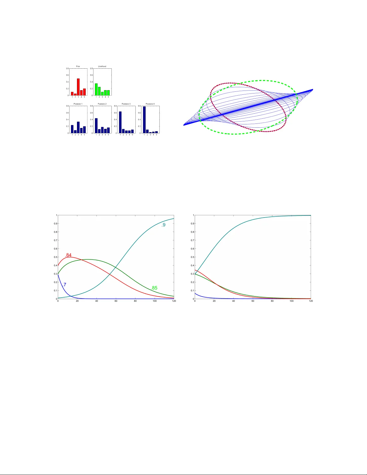
Calculus for Density Ma trices Ba y esian Generalized Probabilit y Calculus for Densit y Matrices ∗ Manfred K. W arm uth manfred@cse.ucsc.edu Dima Kuzmin dima@cse.ucsc.edu Computer Scienc e Dep artment University of California - Santa Cruz Octob er 10, 2007 Editor: Abstract One of the main concepts in quan tum ph ysics is a densit y matrix, which is a symmetric p ositiv e deﬁnite matrix of trace one. Finite probability distributions can b e seen as a sp ecial case when the densit y matrix is restricted to be diagonal. W e develop a probabilit y calculus based on these more general distributions that in- cludes deﬁnitions of join ts, conditionals and form ulas that relate these, including analogs of the Theorem of T otal Probability and v arious Ba yes rules for the calculation of p osterior densit y matrices. The resulting calculus parallels the familiar “con ven tional” probability calculus and alw ays retains the latter as a sp ecial case when all matrices are diagonal. W e motiv ate b oth the con ven tional and the generalized Bay es rule with a minim um relativ e en tropy principle, where the Kullbac h-Leibler v ersion gives the con v entional Ba y es rule and Umegaki’s quan tum relative entrop y the new Bay es rule for densit y matrices. Whereas the conv entional Bay esian metho ds maintain uncertaint y ab out whic h mo del has the highest data lik eliho o d, the generalization maintains uncertaint y ab out which unit direction has the largest v ariance. Surprisingly the b ounds also generalize: as in the con- v entional setting w e upp er b ound the negative log lik eliho o d of the data by the negativ e log lik eliho o d of the MAP estimator. Keyw ords: generalized probabilit y , probabilit y calculus, density matrix, quan tum Bay es rule. 1. In tro duction The main notion of a “mixture state” used in quantum physics is a densit y matrix. States are unit v ectors u ( k u k 2 = 1). F or the sak e of simplicity w e assume in this pap er that the underlying vector space is R n (for ﬁnite n ). Eac h state u (unit column v ector in R n ) is asso ciated with a dyad uu > ∈ R n × n . The dyad uu > ma y be seen as a one-dimensional pro jection matrix whic h pro jects an y vector onto direction u . These dy ads are the ele- men tary even ts of a gener alize d pr ob ability sp ac e . It is useful to k eep the corresp onding “con ven tional” probabilit y space in mind, which consists of a ﬁnite set of size n . The n p oin ts are the elementary even ts and a probabilit y distribution ma y be seen as a mixture ∗ . Supported b y NSF grant IIS 0325363. Some of this w ork was done while visiting National ICT Australia in Canberra. 1 W armuth and Kuzmin Figure 1.1: Tw o diﬀerent dy ad mixtures that lead to the same density ma- trix: 0 . 2 ( 1 0 ) ( 1 0 ) + 0 . 3  √ 2 / 2 √ 2 / 2  ( √ 2 2 √ 2 2 ) + 0 . 5 ( 0 1 ) ( 0 1 ) = ( 0 . 35 0 . 15 0 . 15 0 . 65 ) = 0 . 29  − 0 . 92 0 . 38  ( − 0 . 92 0 . 38 ) + 0 . 71 ( 0 . 38 0 . 92 ) ( 0 . 38 0 . 92 ) . Matrices are depicted as ellipses and dy ads are degenerate single axis ellipses. o ver the n p oints, i.e. such a probability distribution is sp eciﬁed by n real num b ers that are bigger than zero and add to one. In the generalized case there are inﬁnitely man y dyads ev en if the dimension n is ﬁnite. 1 Densit y matrices generalize ﬁnite probability distributions. They can b e deﬁned as mixtures of dy ads W = P i ω i w i w > i where the mixture co eﬃcien ts ω i are non-negative and sum to one. There ma y be an arbitrary n umber of components in the mixture. How ev er, an y n dimensional densit y matrix can be decomp osed in to a mixture of n orthogonal eigendyads , one for each eigenv ector (see Figure 1.1). Mixtures of dy ads are alwa ys symmetric 2 and p ositiv e deﬁnite. A density matrix W can b e depicted as an ellipse whic h is an aﬃne transformation of the unit ball: { W u : || u || 2 = 1 } (See Figure 1.2). A dyad is a degenerate ellipse with a single axis in direction ± u that has radius one (Figure 1.1). Note that dy ads ha ve trace one: tr( uu > ) = tr( u > u ) = k u k 2 2 = 1 . Therefore, densit y matrices also ha ve trace one. A densit y matrix W assigns generalized probability tr( W uu > ) to eac h unit vector u and its asso ciated dy ad uu > (see Figure 1.2). This probability is indep endent of how W is expressed as a mixture and can be rewritten as u > W u . Note that if the symmetric positive deﬁnite matrix A is view ed as a co v ariance matrix of a random cost v ector c , then u > Au is the v ariance of the cost along direction u , i.e. the v ariance of c · u . If α = ( α 1 , . . . , α n ) is a probability v ector, then the n -dimensional matrix diag ( α ) with v ector α as its diagonal is a density matrix. Note that diag( α ) = P i α i e i e > i , where the e i are the standard basis v ectors. Th us conv en tional probability distributions are sp ecial densit y matrices where the eigensystem is restricted to b e the identit y matrix. In this pap er we develop a Bay esian st yle analysis for the case when the eigensystem is allow ed to b e arbitrary . P erhaps the simplest case to see that something unusual is going on is the uniform densit y matrix, i.e. 1 n times iden tity I . This density matrix assigns probability 1 n to ev ery unit v ector, even though there are inﬁnitely man y of them. How ev er, note that the sum of generalized probabilities of an y set of n orthogonal dy ads is n 1 n = 1. As a matter of fact 1. The machinery for inﬁnite dimensional vector spaces is a v ailable. How ever, in this pap er we start with the simplest ﬁnite dimensional setting. 2. In quantum physics complex num bers are used instead of reals. In that case “symmetric” is replaced by “hermitian” and all our formulas hold for that case as well. 2 Calculus for Density Ma trices (a) (b) Figure 1.2: Figure (a) depicts a red ellipse { W u : k u k 2 = 1 } for some density matrix W . The green curve sho ws part of the unit ball. The blue ﬁgure-eight is a plot of the generalized probabilities in direction u , i.e. tr( W uu > ) u . Figure (b) plots a 3-dimensional density matrix (red ellipsoid) and its asso ciated generalized probabilit y surface (in blue). for any densit y matrix W and any set of n orthogonal directions u i , the total generalized probabilit y is one (see Figure 1.3) n X i =1 tr( W u i u > i ) = tr( W X i u i u > i | {z } I ) = tr( W ) = 1 . (1.1) This means that while in the conv en tional case probabilities are additive ov er the p oints in the set, in the generalized case probabilities are additive ov er orthogonal sets of dy ads. In this pap er w e use density matrices as generalized priors and develop a unifying Ba yesian probability calculus for densit y matrices with rules for translating b etw een joints and conditionals. All formulas retain the conv en tional case as the sp ecial case when the matrices are diagonal. In previous w ork (W ar05) w e derived a generalized Ba yes rule based on the minim um relativ e entrop y principle, but no satisfactory probabilistic interpretation w as giv en for this rule. This Ba yes rule ﬁts nicely into our new calculus and w e can interpret it using the notion of generalized probabilit y in tro duced ab ov e. F or an y ﬁxed orthonormal system u i , one can use the dyads u i u > i as elemen tary even ts of a con v entional probabilit y space. As already discussed, an y densit y matrix can be seen as assigning con v entional probabilities to these ev ents that sum to one. Thus if the orthonor- mal system is ﬁxed, generalized probability space is reduced to con ven tional probability space o ver the vectors in the c hosen system. Our approach is fundamentally diﬀerent in that we use densit y matrices to maintain uncertaint y ov er all orthonormal systems. Our conditional densit y matrices are part of the probabilistic system sp eciﬁed by a generalized join t probability distribution. In particular, our conditioning metho d leads to generaliza- tions of the theorem of total probabilit y that in volv e density matrices. In (TR W05) v arious on-line learning up dates w ere generalized from v ector parameters to matrix parameters. F ollo wing (KW97), the updates were derived b y minimizing the loss on the current instance plus a divergence to the last parameter. In this paper w e use the same metho d for deriving a Ba yes rule for densit y matrices, whic h b ecomes the foundation 3 W armuth and Kuzmin (a) (b) Figure 1.3: F or a set of orthogonal directions u i and a density matrix W , the sum of generalized probabilities tr( W u i u > i ) o ver the set is one. Figure (a) shows this for 2-dimensional case: the red ellipse is a densit y matrix W , the blue ﬁgure-eight is a plot of the generalized probablit y tr( W uu > ) around the circle, and for any t wo orthogonal v ectors u 1 and u 2 , tr( W u 1 u > 1 ) + tr( W u 2 u > 2 ) = 1. Figure (b) sho ws the three- dimensional case: for an y three orthogonal directions u 1 , u 2 and u 3 , the probabilities a , b and c of the three asso ciated dy ads sum to one. of our generalized probabilit y calculus. When the parameters are probability vectors o ver the set of mo dels, then the “conv entional” Bay es rule can b e derived using the relativ e en tropy as the divergence (e.g. (Zel98; KW99; SWRL03)). Analogously , we no w use the quan tum relativ e en tropy , in tro duced b y Umegaki, to derive the generalized Ba y es rule. The new rule uses matrix logarithms and exp onentials to av oid the fact that symmetric p ositiv e deﬁnite matrices are not closed under the matrix pro duct. The rule is strikingly similar to the con ven tional Ba yes rule and retains the latter as a sp ecial case when the matrices are diagonal. V arious cancellations o ccur when the conv entional Ba yes rule is applied iteratively and as w e shall see, similar cancellations happ en with the new rule (See Section 9.2). The conv en tional Ba yes rule ma y b e seen as a soft maximum calculation and the new rule as a soft calculation of the eigenv ector with the largest eigenv alue (see ﬁgures 9.1 and 9.2). In ﬁgures 9.3 and 9.4 w e plot the pro jections of p osterior onto the eigendirections of the ﬁxed datalik eliho o d matrix D ( y | M ). The pro jection onto the eigendirection of the largest eigen v alue is a sigmoid like function. The mathematics applied in this pap er are most commonly used in quantum ph ysics. F or example, the assignment of generalized probabilities tr( W uu > ), can b e seen as the outcome of a quan tum measurement of a system in mixture state W being acted up on b y a measurement apparatus describ ed by the dyad uu > . It is tempting to call the new rule the “quantum Ba yes rule”. Ho wev er, w e currently do not hav e a quantum ph ysical in terpretation of this rule. In particular, the state collapse following a measurement does not explicitly app ear in our calculus, also our Ba yes rule can not b e describ ed as a unitary ev olution of the prior state. The term “quan tum Ba yes rule” also has been claimed b efore in (SBC01), where they derive a rule that describ es uncertain ty information about unobserved quan tum measuremen ts of a comp osite system as a density matrix. Our work is most closely related to a paper b y Cerf and Adami (CA99), where, in the con text of quantum information theory , a formula w as prop osed for the conditional density matrix that uses the matrix exponential and matrix logarithm. This sp ecial form ula app ears in our calculus and is no w put in a more general context. W e hop e to transfer many tec hniques developed in Ba yesian Statistics based on the conv en tional Ba yes rule to the con text of generalized probabilities. 4 Calculus for Density Ma trices The pap er is organized as follo ws. Section 2 recalls the relev an t matrix algebra facts. Section 3 in tro duces densit y matrices and generalized probabilit y distributions and states Gleason’s theorem that establishes an equiv alence b etw een them. Then, in Section 4 we in tro duce a generalization  of the matrix pro duct that is commutativ e and preserv es p ositiv e deﬁniteness. This  op eration is central to our calculus. Section 5 introduces generalized joint distributions. Section 6 discusses marginalizing the join ts. Next, in Section 7 we giv e formulas for conditional density matrices. Section 8 presents generalizations of the Theorem of T otal Probabilit y . In Section 9 w e presen t the founding piece of this w ork, the Bay es rule for density matrices, its deriv ation and v arious prop erties. W e also discuss ho w the new Bay es rule for density matrices is in some sense the conv en tional Ba yes rule in an optimally chosen eigensystem. Section 10 summarizes all the rules in our calculus and their justiﬁcations. In the conclusion section w e discuss again ho w our new calculus relates to quan tum ph ysics and p ossible generalizations of it. 2. F acts on Matrices and Basic Notation In this pap er generalized probabilit y distributions, conditionals and data likelihoo ds are represen ted as symmetric p ositive deﬁnite matrices. W e will now discuss some relev an t matrix algebra facts. The basic fact that w e use a lot is the eigendecomp osition of symmetric matrices: S = S σ S > = n X i =1 σ i s i s > i This sa ys that every such matrix can be written as a pro duct of an orthogonal matrix of eigen vectors S times a diagonal matrix of eigen v alues γ times S > . Alternativ ely it can b e written as mixture of eigendyads formed from the eigenv ectors where the eigenv alues act as mixture coeﬃcients. An y symmetric p ositiv e deﬁnite 3 matrix C can b e seen as a cov ariance matrix of some random cost v ector c ∈ R n , i.e. C = E  ( c − E ( c )( c − E ( c )) >  . A cov ariance matrix C can be depicted as an ellipse { C u : k u k 2 = 1 } centered at the origin, where the eigenv ectors form the principal axes and the eigen v alues are the radii of the axes (see Figure 1.2). Note that a co v ariance matrix C is diagonal if the comp onents of the cost v ector are indep enden t. The v ariance of the cost vector c along a vector u , that is the v ariance of the dot product c > u , has the form V ( c > u ) = E  ( c > u − E ( c > u )) 2  = E  (( c > − E ( c > )) u ) > (( c > − E ( c > )) u )  = E  u > ( c − E ( c ))( c − E ( c )) > ) u  = u > C u . The v ariance along an eigen vector of the co v ariance matrix is the corresp onding eigen v alue. Using this interpretation, the matrix C ma y b e seen as a mapping from the unit ball to 3. W e use the conv ention that p ositive deﬁnite matrices hav e non-negative eigenv alues and strictly p ositive deﬁnite matrices hav e p ositiv e eigenv alues. 5 W armuth and Kuzmin R ≥ 0 , i.e. unit v ector u is mapp ed to u > C u . Figure 1.2 depicts the resulting ﬁgure-8-lik e plots in 2 and 3 dimensions. A second interpretation of the scalar u > C u is the square length of u w.r.t. the basis √ C , that is u > C u = u > √ C √ C u = k √ C u k 2 2 . The trace tr( E ) of an arbitrary square matrix E is the sum of its diagonal elemen ts E ii . It is a linear op erator. Recall that tr( E F ) = tr( F E ) for an y matrices E ∈ R n × m , F ∈ R m × n . Also, for symmetric square matrices, tr( S T ) = P i,j S ij T ij , th us trace can be seen as a dot pro duct b etw een matrices. The trace has a useful cycling prop erty: for arbitrary matrices E , F , G with compatible dimensions tr( E F G ) = tr( F GE ) = tr( GE F ). F rom this follo ws that trace is r otation invariant in the sense that for an y orthogonal matrix U , tr( U E U > ) = tr( U > U E ) = tr( E ) . If S is symmetric, setting U to be the eigensystem of S results in the observ ation that trace is equal to the sum of eigenv alues of a matrix. Also, for an y orthogonal system 4 u i , tr( S ) = tr( n X i =1 u i u > i | {z } I S ) = n X i =1 u > i S u i . Therefore if S is symmetric p ositive deﬁnite, then tr( S ) is the total v ariance along an y set of orthogonal directions. Recall that density matrices ha ve trace one and therefore in this case this total v ariance is alw ays one (See Figure 1.3). The matrix exp onential exp ( S ) of the symmetric matrix S = P i σ i s i s > i is computed b y exp onentiating the eigenv alues and lea ving the eigenv ectors unchanged: exp ( S ) = P i exp( σ i ) s i s > i . The matrix logarithm log ( A ) is deﬁned similarly but now A m ust b e strictly p ositive deﬁnite. Clearly , the t wo functions are inv erses of eac h other. It is im- p ortan t to remember that exp ( S + T ) = exp ( S ) exp ( T ) only holds if S and T comm ute i.e. S T = T S . 5 Ho wev er, the follo wing trace inequality , kno wn as the Golden-Thompson inequalit y 6 (Bha97), alw a ys holds: tr( exp ( S ) exp ( T )) ≥ tr( exp ( S + T )) for symmetric S and T , (2.1) where equalit y holds iﬀ b oth symmetric matrices commute. 3. Generalized Probability Distributions and Densit y Matrices In quantum ph ysics a dyad uu > represen ts a pure state and density matrices are mixture states. As w e shall see density matrices can b e in terpreted as generalized probability dis- tributions ov er the set of dy ads. Note that in this pap er we w ant to address the statistics comm unity and use linear algebra notation instead of Dirac notation. Any probabilit y vec- tor ( P ( M i )) can b e represen ted as a diagonal matrix diag( P ( M i )) = P i P ( M i ) e i e > i , where e i denotes the i th standard basis vector. This means that con ven tional probability v ec- tors are sp ecial densit y matrices where the eigenv ectors are ﬁxed to b e the standard basis v ectors. 4. A set of unit v ectors u i is orthogonal iﬀ P i u i u > i = I . 5. This o ccurs iﬀ the t wo symmetric matrices hav e the same eigensystem. 6. Note that the Golden-Thompson inequality do es not generalize to three matrices, i.e. there exist sym- metric S , T , U , s.t. tr( exp ( S ) exp ( T ) exp ( U ))  tr( exp ( S + T + U )). 6 Calculus for Density Ma trices F or the sak e of simplicit y w e assume that our v ector space is R n . Ho wev er, ev erything discussed in this section holds for separable ﬁnite or inﬁnite dimensional real and complex Hilb ert spaces. A function µ ( u ) from unit vectors u in R n to R is called a gener alize d pr ob ability dis- tributions if the following tw o conditions hold: • ∀ u , 0 ≤ µ ( u ) ≤ 1. • If u 1 , . . . , u n form an orthonormal system for R n , then P µ ( u i ) = 1. Gleason’s Theorem states that there is a one-to-one corresp ondence betw een generalized probabilit y distributions and density matrices 7 in R n × n : Theorem 1 (Gle57) L et n ≥ 3 . 8 Then any gener alize d pr ob ability distribution µ on R n has the form µ ( u ) = tr( W uu > ) , for a uniquely deﬁne d density matrix W . It is easy to see that every density matrix deﬁnes a generalized probability distribution. The other direction, is highly non-trivial. 9 As discussed in the in tro duction, the dy ads uu > function as elementary ev ents. One ma y ask what corresp onds to arbitrary even ts and how probabilities are deﬁned for them. In the conv en tional case, an ev ent is a subset of the domain which can be represen ted as a v ector in { 0 , 1 } n . In the generalized setting, an even t is a symmetric p ositive deﬁnite matrix P with eigenv alues in { 0 , 1 } . Eac h such matrix P with eigendecomp osition P k i =1 p i p > i is a pro jection matrix for a subspace of R n and its probabilit y w.r.t. a distribution W is deﬁned as the sum of the probabilities of the elemen tary ev ents p i p > i comprising P : tr( W P ) = k X i =1 tr( W p i p > i ) . In terpreting P as a cov ariance matrix of some random v ariable, w e can also expand W and sum the v ariance along its eigendirections w i w eighted by the eigenv alues ω i whic h are probabilities: tr( W P ) = tr( n X i =1 ω i w i w > i P ) = n X i =1 probability z}|{ ω i v ariance z }| { w > i P w i | {z } expected v ariance . (3.1) Random v ariables are deﬁned in an analogous wa y . In the con v entional case a random v ariable asso ciates a real v alue with each p oin t. Now a random v ariable is an arbitrary symmetric matrix S . Such matrices hav e arbitrary real n um b ers as their eigenv alues and trace tr( W S ) when S is expanded b ecomes the exp ectation of the random v ariable w.r.t. densit y W : tr( W S ) = tr( W X i σ i s i s > i ) = X i outcome z}|{ σ i probability z }| { s > i W s i | {z } expected outcome . (3.2) 7. The core of the original pro of of Gleason’s Theorem w as for R 3 (Gle57), and he then generalized the pro of to separable real and complex Hilb ert spaces of dimension n ≥ 3. 8. A sligh tly diﬀerent version of this theorem that is base d on “eﬀects” instead of dyads holds for dimension 2 as well (CFMR04). 9. Ho wev er, if dyads are replaced by “eﬀects” then the proofs are m uch simpler (CFMR04). 7 W armuth and Kuzmin As discussed b efore, the con ven tional case of the exp ectation calculation is alw ays retained as a special case when all the matrices are diagonal (i.e. ﬁxed eigensystem I ). In quan tum ph ysics the exp ectation calculation tr( W S ) has the follo wing interpretation: an instrument is represen ted by a hermitian matrix S and tr( W S ) is the e xp ected v alue of a quantum me asur ement of the mixed state W with instrumen t S . The eigen v alues σ i of the instrumen t represen t the p ossible n umerical measuremen t outcomes. Each one of those outcomes is observ ed with probabilit y s > i W s i , where s i is the asso ciated eigenv ector of the instrumen t matrix S . In real quantum systems the measuremen t causes the mixtures state W to c ol lapse in to one of the orthogonal states { s 1 s > 1 , . . . , s n , s > n } : the successor state is s i s > i with probabilit y s > i W s i : W measurement − → collapse X i probability z }| { s > i W s i s i s > i | {z } expected state . As we shall see, the exp ected measurement calculations pla y an imp ortant part in our calculus. Ho wev er our up date rules for densit y matrices (suc h as our Bay es rule) do not explicitly include a collapse in the ab ov e sense. Note that some of the equations ab o ve hold for arbitrary decomp ositions in to a linear com bination of dyads of any size. F or example (3.1), holds for an y decomp osition W = P i ω i w i w > i , i.e. the ω i ma y b e negative, the w i ma y b e non-orthogonal, and the size of the decomp osition may be larger than n . If the ω i are non-negative, then they form a probability v ector. Similarly , (3.2) also holds for any decomp osition S = P i σ i s i s > i . How ev er, quan tum measuremen ts are alwa ys based on an orthogonal system. F urthermore, orthogonal systems are sp ecial in that the orthogonal decomp osition of a density matrix W = P i ω i w i w > i attains the minimum of the en tropy P i − ω i ln ω i o ver all p ossible decomp ositions of W (Inequalit y (11.86) in (NC00)). A question that naturally arises is whether w e can mo del the generalized probabilit y distributions deﬁned ab o ve with a con v entional probabilit y space. In other words, is there a con ven tional probabilit y space and t wo mappings: one that maps densit y matrices to con- v entional probabilit y distributions and the other mapping dy ads to ev en ts of this probability space. The requirement on these t wo mappings is that the conv en tional probability calcu- lations using the images of density matrices and dyads under these mappings satisfy the deﬁnition of the generalized probabilit y distributions giv en ab ov e. Essentially , it is kno wn that conv en tional probability spaces cannot satisfactorily mo del generalized probabilities, but the details are rather inv olv ed. This topic has receiv ed considerable attention in the quan tum ph ysics communit y and we refer readers to (Hol01) for an extended discussion of imp ossibilit y results. Here we only give one simple attempt to mo del density matrices with a conv entional probabilit y space and sho w that the t wo natural mappings fail to satisfy the requiremen ts. A natural in terpretation of a densit y matrix is to view it as a parameterized densit y o ver the unit sphere. W e claim that if µ ( u ) is the uniform density on the sphere, then for an y symmetric p ositiv e deﬁnite matrix A ∈ R n × n of trace n , u > A u µ ( u ) is also a conv entional 8 Calculus for Density Ma trices probabilit y densit y on the sphere: Z u > A z }| { X i α i a i a > i u µ ( u ) d u = X i α i Z ( u > a i ) 2 µ ( u ) d u = tr( A ) Z ( u > ( 1 √ n , . . . , 1 √ n ) > ) 2 µ ( u ) d u = tr( A ) n Z 1 z }| { ( u ) 2 µ ( u ) d u | {z } 1 . In the second equality we used the fact that µ ( u ) d u is uniform and therefore the in tegral of ( u > a i ) 2 is the same as the integral of the squared dot pro duct of u with uniform vector ( 1 √ n , . . . , 1 √ n ) > . W e modeled density matrices as con v entional probabilit y densities ov er the sphere. No w the natural mapping from dy ads to even ts in the con ven tional probabilit y space (the sphere) maps uu > to { u , − u } . How ev er the probabilit y of the latter sets of size 2 is zero with resp ect to the conv en tional probabilities densities w e deﬁned on the sphere. In particular the probabilit y on any n orthogonal dy ads does not sum to one. 4. Commutativ e Matrix Pro duct Op eration It is well kno wn that the pro duct of t wo symmetric p ositiv e deﬁnite matrices might b e neither symmetric nor p ositive deﬁnite (see Figure 4.1). In this section w e deﬁne a commu- tativ e “pro duct” op eration b etw een symmetric p ositive deﬁnite matrices that do es result in a symmetric p ositiv e deﬁnite matrix. Our ﬁrst deﬁnition of this op eration requires the t wo matrices to b e strictly p ositiv e deﬁnite. W e then extend the deﬁnition to arbitrary symmetric positive deﬁnite matrices and prov e man y properties of this pro duct. F or tw o symmetric and strictly p ositive deﬁnite matrices A and B , w e ﬁrst deﬁne the  as: A  B := sym.pos.def. z }| { exp ( sym. z }| { log sym.pos.def. z}|{ A + sym. z }| { log sym.pos.def. z}|{ B ) , (4.1) where here the exp onential and logarithm are matrix functions. The matrix log of b oth matrices pro duces symmetric matrices whic h are closed under addition and the matrix exp onen tial of the sum returns a symmetric p ositive deﬁnite matrix. See Figure 4.1 for a comparison of matrix pro duct and  . Note that we expressed the op eration  b etw een symmetric strictly p ositive deﬁnite matrices as a + op eration b etw een symmetric matrices. Similarly , for any tw o arbitrary symmetric matrices S and T , S + T = log ( exp ( S )  exp ( T )) . The op eration  was used in (Ale02) to deﬁne a “pro duct” b etw een tw o linear transfor- mations that is commutativ e. In this pap er w e use  to deﬁne conditional density matrices 9 W armuth and Kuzmin Figure 4.1: The matrix pro duct of t w o positive deﬁnite matrices do es not preserv e p ositive deﬁniteness. F or t wo matrices A and B we plot their ellipses Au , B u and ﬁgure eigh ts tr( Auu > ) u , tr( B uu > ) u (for unit u ). Both ellipses are very thin, i.e. the ratio b etw een the t wo eigenv alues of eac h matrix is 100. W e also plot the ellipse AB u and the curv e tr( AB uu > ) u . The latter curve consists of t wo ﬁgure eights, the larger one constitutes the part where the trace is positive and the smaller and skinnier one is the part where the trace is negativ e. This means that AB is not p ositiv e deﬁnite any more. The pro duct is also not symmetric b ecause the min/max v alue of tr( AB uu > ) do es not corresp ond to the axes of the ellipse. Finally , the corresp onding plots for A  B indicate that this matrix is symmetric and p ositive deﬁnite. Figure 4.2: When the ellipses A and B don’t ha ve the same span, then A  B lies in the in- tersection of b oth spans. In the depicted case the in tersection is a degenerate ellipse of dimension one (blue line). This generalizes the following in tersection prop erty of the matrix pro duct when A and B are b oth diagonal (here of dimen- sion four): ( AB ) i,i 6 = 0 iﬀ A i,i 6 = 0 and B i,i 6 = 0 . diag( A ) diag( B ) diag( AB ) 0 0 0 a 0 0 0 b 0 a b ab and generalizations of the Bay es rule. A similar path w as follow ed by (CA99) for deﬁn- ing conditional density matrices of comp osite systems. W e also give a motiv ation for the op eration based on the minimum relativ e en tropy principle (as was done in the conference pap er (W ar05)) and our probability calculus includes the form ula of (CA99) for comp osite systems as a sp ecial case. Note that the form ula for  in Equation (4.1) is not deﬁned if some of the eigen v alues of A or B are zero. W e no w rewrite the op eration using the Lie-T rotter formula and then extend it to arbitrary p ositive deﬁnite matrices. The Lie-T rotter formula (see e.g. (Bha97)) is the following equation: exp ( E + F ) = lim n →∞ ( exp ( E /n ) exp ( F /n )) n , an y square matrices E , F . 10 Calculus for Density Ma trices Figure 4.3: The b ehavior of the limit form ula for  operation. W e can see that the additional ﬁgure eigh ts indicating negativ e deﬁniteness are smaller for ( A 1 / 2 B 1 / 2 ) 2 than for AB . As n increases, the additional ﬁgure eigh ts shrink further and lim n →∞ ( A 1 /n B 1 /n ) n = A  B b ecomes positive deﬁnite. Also, AB and B A are fairly diﬀerent from one another. The matrices ( A 1 / 2 B 1 / 2 ) 2 and ( B 1 / 2 A 1 / 2 ) 2 are already more similar and the diﬀerence b etw een the tw o multiplication orders decreases with n until in the limit A  B = B  A . By choosing E = log A and F = log B , for symmetric and strictly positive deﬁnite A and B , we obtain: exp ( log A + log B ) = lim n →∞ ( A 1 /n B 1 /n ) n . As n increases, ( A 1 /n B 1 /n ) n gets closer and closer to b eing positive deﬁnite and symmetric. The ﬁrst couple iterations of the limit formula are plotted in Figure 4.3. See (Ale02) for additional plots. Notice that the limit is deﬁned ev en when A and B hav e zero eigenv alues. W e therefore extend the deﬁnition of  to arbitrary symmetric p ositive deﬁnite matrices A and B : A  B := lim n →∞ ( A 1 /n B 1 /n ) n . (4.2) F rom now on we use the ab o ve exended deﬁnition of  . Numerous prop erties of this op eration are given b elow. Theorem 2 F or any symmetric p ositive deﬁnite matric es A , B , C the fol lowing holds: OP1. Interse ction pr op erty: range( A  B ) = range( A ) ∩ range( B ) . wher e the r ange of a matrix is the line ar subsp ac e sp anne d by the c olumns of the matrix. This pr op erty gener alizes the interse ction pr op erties for pr o ducts of diago- nal matric es (which mo del c onventional pr ob ability distributions): the pr o duct of two diagonal matric es with the char acteristic ve ctors of two subsets as diagonals gives a diagonal matrix forme d fr om the char acteristic ve ctor of the interse ction (Se e Figur e 4.2). OP2. L et R A b e a matrix whose c olumns form an orthonormal b asis for the r ange of A , i.e. R A ∈ R n × k and R > A R A = I k , wher e k is the dimensionality of the r ange of A . Deﬁne R B analo gously. In a similar fashion R A ∩ B wil l c ontain the b asis for the interse ction of r anges. L et log + denote the mo diﬁe d matrix lo garithm that takes the 11 W armuth and Kuzmin lo g of non-zer o eigenvalues but le aves the zer o eigenvalues unchange d. This op er ation c an b e also deﬁne d by the fol lowing formula: 10 log + A = R A log ( R > A AR A ) R > A . (4.3) With this notation,  c an b e written as A  B = R A ∩ B exp ( R > A ∩ B ( log + A + log + B ) R A ∩ B ) R > A ∩ B . (4.4) OP3. A  B = AB if A and B c ommute. OP4.  is c ommutative, i.e. A  B = B  A . OP5. The identity matrix is the neutr al element, i.e. A  I = A . OP6. ( c A )  B = c ( A  B ) , for any sc alar c > 0 . OP7. A  A − 1 = I for invertible A . A lso, A  A + = P A , wher e A + denotes the pseudoin- verse and P A is the pr oje ction matrix 11 for range( A ) . OP8.  is asso ciative, i.e. ( A  B )  C = A  ( B  C ) . OP9. Monotonic c onver genc e of the limit deﬁning  : ∀ n ≥ 1 : tr( A 1 / ( n +1) B 1 / ( n +1) ) n +1 ≤ tr( A 1 /n B 1 /n ) n . OP10. tr( A  B ) ≤ tr( AB ) , wher e e quality holds iﬀ A and B c ommute. In p articular, for any unit u tr( A  uu > ) = tr( Auu > ) iﬀ u is an eigenve ctor of A . OP11. F or any unit dir e ction u ∈ range( A ) , A  uu > = e u > ( log + A ) u uu > . OP12. F or any unit dir e ction u and eigende c omp osition P i α i a i a > i of a strictly p ositive def- inite matrix A , tr( Auu > ) = X i ( u > a i ) 2 α i , and tr( A  uu > ) = Y i α ( u > a i ) 2 i , i.e. the matrix pr o duct c orr esp onds to an arithmetic aver age and the  pr o duct to a ge ometric aver age of the eigenvalues of A . OP13. det( A  B ) = det( A ) det( B ) , which is the same as for the normal matrix pr o duct. OP14. F or any ortho gonal system u i , we have Q i tr( A  u i u > i ) = det( A ) . 10. Note that when the rank k of A is zero, then one still can deﬁne the pro jections in a consistent manner. In this case R A is of dimension n × 0, and the matrices R > A R A and log ( R > A E R A ) are of dimension 0 × 0 for any E ∈ R n × n . Also it is natural to deﬁne R A E R > A as the n × n zero matrix 0 . With this deﬁnition, the r.h.s. of (4.3) is 0 when A is 0 . 11. Note that P A = R A R > A . 12 Calculus for Density Ma trices OP15. F or any unit dir e ction u , tr(( A  B )  uu > ) = tr( A  uu > ) tr( B  uu > ) . OP16. F or any unit dir e ction u ∈ range A , tr( A +  uu > ) = 1 tr( A  uu > ) , wher e A + denotes the pseudoinverse. Pro of Prop erties OP1 and OP2 follo w from results in (Kat78) or Theorem 1.2 of (Sim79). Here we only prov e that range( A  B ) ⊆ range( A ) ∩ range( B ). W e can split the limit deﬁning  as follo ws: A  B = lim n →∞ ( A 1 /n B 1 /n ) n = lim n →∞ A 1 /n lim n →∞ B 1 /n ( A 1 /n B 1 /n ) n − 1 . (4.5) Here w e used the prop erty that lim E n F n = lim E n lim F n if all the limits exist. This follo ws from the corresponding sum and product prop erties of scalar limits and the fact that en tries of a pro duct matrix are ﬁnite sums of pro ducts. It is easy to see that lim n →∞ A 1 /n = P A b ecause the matrix p ow er for a symmetric matrix corresp onds to taking p ow ers of the eigenv alues and n -th ro ots conv erge to either zero or one. Thus the limit is a matrix whose eigenv alues are 0 or 1, which is a pro jection matrix. By plugging lim n →∞ A 1 /n = P A = P A P A = P A lim n →∞ A 1 /n in to (4.5) w e get A  B = P A lim n →∞ A 1 /n lim n →∞ B 1 /n ( A 1 /n B 1 /n ) n − 1 = P A ( A  B ) . This implies that range( A  B ) ⊆ range( A ). Similarly w e can prov e A  B = ( A  B ) P B , whic h implies that range( A  B ) ⊆ range( B ), and therefore range( A  B ) ⊆ range( A ) ∩ range( B ). Prop ert y OP3 can b e seen from the deﬁnition of  via the limit formul a (4.2): when A and B commute, then the n copies of A 1 /n in ( A 1 /n B 1 /n ) n can b e gathered in to A and similarly for B 1 /n . Prop erties 4 - 7 easily follow from the form ula (4.4) for  . Prop ert y OP8. F or strictly p ositive deﬁnite A , B , C asso ciativity reduces to the asso- ciativit y of addition in the log domain. T o show it in general we use the representation (4.4) of  via the log + op eration. Let R = R ( A ∩ B ) ∩ C = R A ∩ ( B ∩ C ) . Then: ( A  B )  C = R exp ( R > ( log + ( A  B ) + log + C ) R ) R > No w w e rewrite log + ( A  B ) using Equation (4.3): log + ( A  B ) = R A ∩ B log ( R > A ∩ B ( A  B ) R A ∩ B ) R > A ∩ B Substituting expression (4.4) for A  B into the ab ov e and using R > A ∩ B R A ∩ B = I k w e get: log + ( A  B ) = R A ∩ B R > A ∩ B | {z } P A ∩ B ( log + A + log + B ) R A ∩ B R > A ∩ B | {z } P A ∩ B . (4.6) 13 W armuth and Kuzmin Here P A ∩ B = R A ∩ B R > A ∩ B is the pro jection matrix on to the subspace range( A ) ∩ range( B ). All the basis v ectors of A ∩ B ∩ C ob viously lie in the larger subspace as well, thus the pro jection lea v es them unc hanged and we get P A ∩ B R = R , R > P A ∩ B = R > . Th us: ( A  B )  C = R exp ( R > ( log + A + log + B + log + C ) R ) R > . The same expression can be obtained for A  ( B  C ), thus establishing asso ciativit y . Prop ert y OP9. By F act 8.10.9 of (Ber05), w e ha v e that for any p ositive deﬁnite matrices A and B , and n ≥ 1: tr( A n B n ) n +1 ≤ tr( A n +1 B n +1 ) n . No w b y substituting A = A 1 / ( n ( n +1)) , B = B 1 / ( n ( n +1)) the monotonicity prop erty OP9 immediately follo ws. Prop ert y OP10. When A and B are strictly p ositive deﬁnite, this inequalit y is an instan tiation of the Golden-Thompson inequalit y (2.1). F or arbitrary positive deﬁnite ma- trices, the property follo ws from the previous monotonicit y prop erty OP9. Note that there are symmetric p ositive deﬁnite matrices A , B and C s.t. tr( A  B  C )  tr( AB C ). Prop ert y OP11. W e use the expression for  op eration given in Equation (4.4). Since u ∈ range( A ), the basis of the in tersection space is u itself: uu >  A = u exp ( u > ( log + uu > + log + A ) u ) u > . Note that log + uu > = 0 and that the expression inside the exp onential is a scalar. The desired property immediately follo ws b y mo ving this scalar to the fron t. Prop ert y OP12. The expression for the trace of the matrix pro duct is the exp ected measuremen t interpretation (3.2) discussed in Section 3. Note that ( u > a i ) 2 is a probability v ector and in this expression uu > can be replaced b y an y densit y matrix. F or the second trace tr( A  uu > ), we can rewrite it using OP11 and eigendecomposition of A as follo ws: tr( A  uu > ) = e u > log Au = e P i ( a i · u ) 2 log α i = Y i α ( u > a i ) 2 i , whic h is a weigh ted geometric av erage of α i with w eigh ts ( u > a i ) 2 . Prop ert y OP13. Since det( E F ) = det( E ) det( F ), and for symmetric matrices S and r ∈ R , det( S r ) = det( S ) r , w e hav e det(( A 1 /n B 1 /n ) n ) = det( A ) det( B ) for all n ∈ N . By Prop ert y (4.2), the limit of the l.h.s. of the last equality b ecomes A  B and this pro v es the property . Prop ert y OP14. If A is not full rank, then det( A ) is zero. In that case, there will be some u i that is not in the range of A . F or that u i , tr( A  u i u > i ) = 0, making the whole pro duct zero. When A has full rank, we rewrite the pro duct as follo ws: Y i tr( A  u i u > i ) OP 11 = Y i e tr( log Au i u > i ) = e tr( log A P u i u > i ) = e tr( log A ) = Y i α i = det( A ) . 14 Calculus for Density Ma trices Prop ert y OP15. If u / ∈ range( A ) ∩ range( B ) (OP1) = range( A  B ), then the prop erty trivially holds b ecause tr(( A  B )  uu > ) and either tr( A  uu > ) or tr( B  uu > ) are zero. When u ∈ range( A ) ∩ range( B ), then the prop erty essentially follows from e a + b = e a e b : tr(( A  B )  uu > ) OP 11 = e u > log + ( A  B ) u (4.6) = e u > P A ∩ B ( log + A + log + B ) P A ∩ B u = e u > ( log + A + log + B ) u = e u > log + Au e u > log + B u = tr( A  uu > ) tr( B  uu > ) . Needless to say Prop erty OP15 do es not hold if uu > is replaced by a mixture of dyads. Prop ert y OP16. T rivially follo ws from OP11. W e will now discuss some of the prop erties further. In particular, we will show a simple example that demonstrates that the upp er b ound OP10 can b e quite lo ose when b oth matrices are dyads. In this case the inequality b ecomes: tr( uu >  v v > ) ≤ tr( uu > v v > ) = ( u · v ) 2 . The righ t hand side can b e made arbitrarily close to one by c ho osing almost parallel u and v . The left side is zero in this case, whic h can b e seen b y analyzing the in tersection of the ranges. Dyads are rank one matrices and their ranges are lines through the origin. The in tersection of t w o such lines is either only the origin or the line itself. Thus, by Prop ert y (OP1) it follo ws that uu >  v v > = 0 , unless u = ± v . This can also b e seen from the limit expression in Equation (4.2): uu >  v v > = lim n →∞ (( uu > ) 1 n ( v v > ) 1 n ) n = lim n →∞ ( uu > v v > ) n =  lim n →∞ ( u · v ) 2 n − 1  uv > = 0 , unless u = ± v . Where the last equalit y holds because | u · v | < 1, when u 6 = ± v . Note that the expression (4.4) for  based on log + giv es us a conv enien t metho d for computing the op eration even when the matrices hav e some zero eigenv alues. The mo diﬁed matrix logarithm log + is easily computed via Equation (4.3). The matrix R A con taining the orthonormal basis for range of A can b e computed using Gram-Schmidt orthogonalization pro cedure or the QR-decomp osition. T o compute the basis for the in tersection of range( A ) and range( B ), we express the in tersection i.t.o. the union and the orthogonal complemen t ⊥ of a space: range( A ) ∩ range( B ) =  range( A ) ⊥ ∪ range( B ) ⊥  ⊥ . F or an y matrix E , an orthonormal basis for range( E ) ⊥ can b e obtained by com pleting an orthonormal basis for range( E ) to an orthonormal basis for the whole space. The additional basis v ectors needed are the basis for range( E ) ⊥ . Also, if w e ha ve t w o matrices E and F , w e can get the range for the union of their ranges just b y putting all columns of E and F together in to a bigger matrix G = ( E , F ). Clearly , range( G ) = range( E ) ∪ range( F ). Piecing all of this together gives an implemen tation of the  op eration. 15 W armuth and Kuzmin 5. Joint Distributions A density matrix deﬁnes a generalized probabilit y distribution ov er the dyads from one space. How ev er w e need to consider several spaces and join t distributions ov er them. In the conv en tional case A, B denote ﬁnite sets { a 1 , . . . , a n A } , { b 1 , . . . , b n B } , ( P ( a i )) , ( P ( b j )) probabilit y vectors o v er these sets and ( P ( a i , b j )) is an n A × n B dimensional matrix of prob- abilities for the tuple set A × B . In the generalized case, A , B denote real ﬁnite dimensional v ector spaces of dimension n A , n B and D ( A ) , D ( B ) are the density matrices deﬁning the generalized probability distributions o ver these spaces. The joint sp ac e ( A , B ) is the tensor pro duct 12 b et ween the spaces A and B , whic h is of dimension n A n B . The joint distribution is speciﬁed b y a densit y matrix ov er this joint space, denoted b y D ( A , B ). W e let D ( a ) , D ( b ) denote the probabilities assigned to dyads aa > , bb > from the spaces A , B b y the density matrices D ( A ) , D ( B ), resp ectiv ely: D ( a ) := tr( D ( A ) aa > ) , D ( b ) := tr( D ( B ) bb > ) . (MJ1) The conv en tional probability distributions can b e seen as diagonal density matrices. A probabilit y distribution ( P ( a i )) on the set A is the density matrix diag(( P ( a i ))). Also P ( a j ) = e > j diag(( P ( a i ))) e j . T o introduce the joint probabilit y D ( a , b ) w e need the Kronec ker matrix pro duct. Given t wo matrices E and F with dimensions n × m and p × q , their Kroneck er pro duct (also kno wn as direct pro duct or tensor pro duct) E ⊗ F is a matrix with dimensions np × mq whic h in block form is giv en as:     e 11 F e 12 F . . . e 1 m F e 21 F e 22 F . . . e 2 m F . . . . . . . . . . . . . . . . . . . . . . . . . e n 1 F e n 2 F . . . e nm F     . The Kronec k er pro duct has the following useful properties: KP1. ( E ⊗ F ) > = E > ⊗ F > . KP2. ( E ⊗ F )( G ⊗ H ) = E G ⊗ F H if the dimensions are appropriate. KP3. tr( E ⊗ F ) = tr( E )tr( F ). KP4. If symmetric matrix S has eigenv alues σ i and eigen v ectors s i and symmetric matrix T has eigen v alues τ j and eigen vectors t j , then S ⊗ T has eigenv alues σ i τ j and eigen vectors s i ⊗ t j . KP5. F or symmetric p ositive deﬁnite matrices A , B , C , D , ( A ⊗ B )  ( C ⊗ D ) = ( A  C ) ⊗ ( B  D ). 12. See (Bha97) for a formal deﬁnition of tensor pro duct b et ween vector spaces. F or us, the tensor pro duct of R n A and R n B is R n A n B . 16 Calculus for Density Ma trices The ﬁrst four prop erties are standard. The last property follows from the limit deﬁnition (4.2) of the  operation. ( A ⊗ B )  ( C ⊗ D ) = lim n →∞  ( A ⊗ B ) 1 n ( C ⊗ D ) 1 n  n = lim n →∞  ( A 1 n C 1 n ) ⊗ ( B 1 n D 1 n )  n =  lim n →∞ ( A 1 n B 1 n ) n  ⊗  lim n →∞ ( C 1 n D 1 n ) n  The last transition which mov ed the limit inside the Kroneck er pro duct, follo ws from the fact that the elemen ts of the Kronec ker pro duct matrix are just pairwise products of elements from the tw o matrices. And when all limits exist, a limit of a pro duct of tw o num b er sequences is a pro duct of limits. No w the joint probability D ( a , b ) b ecomes the probability assigned b y densit y matrix D ( A , B ) to the jointly sp eciﬁed dy ad ( a ⊗ b )( a ⊗ b ) > : D ( a , b ) := tr( D ( A , B )( a ⊗ b )( a ⊗ b ) > ) = tr( D ( A , B )( aa > ⊗ bb > )) . (MJ3) Note that in the conv entional case a join t b etw een t wo sets A and B is deﬁned ov er all pairs of points from A and B . How ev er, in the generalized case, there are elemen tary ev en ts in the join t space that don’t decompose into elemen tary even ts of the marginal densit y matrices, i.e. there are dyads in the joint space that are not of the form ( a ⊗ b )( a ⊗ b ) > . This is what quan tum ph ysicists call “en tanglemen t”. 6. Marginalization of the Joint via P artial T races W e would like to b e able to p erform marginalization op erations on our joint density matrix D ( A , B ), i.e. obtain the density matrix D ( A ) from the join t matrix. In the conv en tional case the marginalization w as performed b y summing out one of the v ariables b y summing the rows or the columns of the matrix sp ecifying the joint probabilit y distribution. F or densit y matrices, the analogous op eration is the p artial tr ac e (see e.g. (NC00)). The partial trace is a generalization of normal matrix trace. It t ypically pro duces a matrix instead of a n um b er and can be used to retrieve the (scaled) factor matrices from a Kronec ker pro duct. W e denote the partial trace with tr A , where A sp eciﬁes the space to b e “summed out”. Supp ose G is a matrix o ver the space A ⊗ B and A has dimension n and B dimension m . Thus G has dimension nm × nm and can b e written in blo c k form as a n × n matrix of m × m matrices G ij : G =     G 11 G 12 . . . G 1 n G 21 G 22 . . . G 2 n . . . . . . . . . . . . . . . . . . . . . G n 1 G n 2 . . . G nn     Here we supp ose that space A is R n and space B is R m . Then the tw o partial traces of this matrix are given by: tr A ( G ) | {z } m × m = G 11 + G 22 + . . . + G nn 17 W armuth and Kuzmin tr B ( G ) | {z } n × n =     tr( G 11 ) tr( G 12 ) . . . tr( G 1 n ) tr( G 21 ) tr( G 22 ) . . . tr( G 2 n ) . . . . . . . . . . . . . . . . . . . . . . . . . . . . . . . . tr( G n 1 ) tr( G n 2 ) . . . tr( G nn )     In multilinear algebra partial traces are known as tensor con tractions and can of course b e generalized to the tensor pro duct of more than tw o spaces. The partial trace is a linear op erator and we now give some other useful prop erties: PT1. tr A ( E ⊗ F ) = tr( E ) F , tr B ( E ⊗ F ) = tr( F ) E . PT2. tr( G ) = tr(tr A ( G )) = tr(tr B ( G )). PT3. tr A ( G ( I A ⊗ F )) = tr A ( G ) F , tr A (( I A ⊗ F ) G ) = F tr A ( G ). PT4. tr( G ( E ⊗ F )) = tr(tr B ( G ( I A ⊗ F )) E ). The ﬁrst three prop erties are straigh tforward and the last one follows from the others as follo ws: tr( G ( E ⊗ F )) K P 2 = tr( G ( I A ⊗ F )( E ⊗ I B )) = tr(( E ⊗ I B ) G ( I A ⊗ F )) P T 2 = tr(tr B (( E ⊗ I B ) G ( I A ⊗ F ))) P T 3 = tr( E tr B ( G ( I A ⊗ F )) . W e use the partial trace to deﬁne marginals as follo ws: D ( A ) := tr B ( D ( A , B )) , D ( B ) := tr A ( D ( A , B )) (MJ2) The follo wing lemma shows that D ( A ) and D ( B ) deﬁned this wa y are again densit y matri- ces. Lemma 3 Partial tr ac e of a density matrix is also a density matrix. Pro of Symmetry is obvious. T race one follo ws from Prop ert y PT2 of the partial trace: tr( D ( A )) = tr(tr B ( D ( A , B ))) = tr( D ( A , B )) = 1 . P ositive deﬁniteness follo ws b y a similar argument: a > D ( A ) a = tr( D ( A ) aa > ) P T 3 = tr(tr B ( D ( A , B )( aa > ⊗ I B ))) P T 2 = tr( D ( A , B )( aa > ⊗ X i b i b > i | {z } I B )) = X i tr( D ( A , B )( aa > ⊗ b i b > i )) = X i ( a ⊗ b i ) > D ( A , B )( a ⊗ b i ) ≥ 0 . P artial traces also allow us to deﬁne ob jects of the type D ( A , b ). In the conv en tional case 18 Calculus for Density Ma trices this corresp onds to taking one row or column out of the joint probability table. In the generalized case we wan t the following prop erty to b e satisﬁed: tr( D ( A , b ) aa > ) = D ( a , b ) . (MJ5) This is accomplished b y deﬁning D ( A , b ) via the follo wing form ula: D ( A , b ) := tr B ( D ( A , B )( I A ⊗ bb > )) . (MJ4) Prop ert y MJ5 now follows from partial trace Prop ert y PT4. W e can also see that trace of D ( A , b ) giv es us the probability D ( b ): tr( D ( A , b )) MJ4 = tr(tr B ( D ( A , B )( I A ⊗ bb > ))) P T 2 = tr(tr A ( D ( A , B )( I A ⊗ bb > ))) (6.1) P T 3 = tr(tr A ( D ( A , B )) bb > ) MJ2 = tr( D ( B ) bb > ) = D ( b ) . A brief note on matrix prop erties of D ( A , b ). W e just saw that its trace is D ( b ) whic h is b etw een zero and one. Since it satisﬁes Prop erty (MJ5), it is p ositiv e deﬁnite as well. Symmetry is also easily v eriﬁed. Note that for an y orthogonal system b i of B , D ( A ) = X i D ( A , b i ) . This can b e seen as follows. D ( A ) MJ2 = tr B ( D ( A , B )) = tr B ( D ( A , B )( I A ⊗ I B )) = tr B ( D ( A , B )( I A ⊗ X i b i b > i | {z } I B )) = X i tr B ( D ( A , B )( I A ⊗ b i b > i )) MJ4 = X i D ( A , b i ) . The conv en tional deﬁnition of indep endence also naturally generalizes: D ( A ) is indep endent of D ( B ) if the joint densit y matrix decomp oses: D ( A , B ) = D ( A ) ⊗ D ( B ). It is easy to see that in this case w e ha v e D ( a , b ) = D ( a ) D ( b ) for all a , b : D ( a , b ) = tr(( D ( A ) ⊗ D ( B ))( aa > ⊗ bb > )) K P 2 = tr(( D ( A ) aa > ) ⊗ ( D ( B ) bb > )) K P 3 = tr( D ( A ) aa > )tr( D ( B ) bb > ) = D ( a ) D ( b ) . 7. Conditional Probabilities The topic of conditional probabilities in this generalized setting con tains man y subtleties. First we will giv e the deﬁning formulas for conditional densit y matrices and then discuss some of the issues. CP1. D ( A | B ) := D ( A , B )  ( I A ⊗ D ( B )) − 1 (F orm ula (4) of (CA99) expressed with the  op eration). This form ula requires D ( B ) to be in vertible. In the con v entional case, this corresp onds to the conditional probabilities b eing undeﬁned if the ev en t conditioned on has probability zero. 19 W armuth and Kuzmin CP2. D ( A | b ) := D ( A , b ) D ( b ) . CP3. D ( a | B ) := D ( a , B )  D ( B ) − 1 . CP4. D ( a | b ) := D ( a , b ) D ( b ) . This basic conditional probability is a straightforw ard generaliza- tion of the conv en tional case. It also has a quan tum-mechanical interpretation. See App endix A for details. Note that CP1 has the form: density matrix  inv erse of a normalization. W e can also reexpress the other deﬁnitions in this uniﬁed form: CP 0 2. D ( A | b ) = tr B ( D ( A , B )( I A ⊗ bb > )) | {z } D ( A , b )  tr B (( I A ⊗ D ( B ))( I A ⊗ bb > )) − 1 | {z } 1 D ( b ) I A . CP 0 3. D ( a | B ) = tr A ( D ( A , B )( aa > ⊗ I B )) | {z } D ( a , B )  tr A (( I A ⊗ D ( B ))( aa > ⊗ I B )) − 1 | {z } D ( B ) − 1 . CP 0 4. D ( a | b ) = tr( D ( A , B )( aa > ⊗ bb > )) | {z } D ( a , b )  tr(( I A ⊗ D ( B ))( aa > ⊗ bb > )) − 1 | {z } 1 D ( b ) . W e say that the join t densit y D ( A , B ) is de c ouple d if its eigendecomp osition has the form: D ( A , B ) = ( W A ⊗ W B ) diag( ω )( W A ⊗ W B ) > . Note that W A ⊗ W B is orthogonal iﬀ b oth W A and W B are orthogonal. As we shall see later, dealing with conditionals is often simpler in the decoupled case. W e ﬁrst prov e an upp er b ound for tr( D ( A | B )) that is tigh t iﬀ the joint is decoupled. Lemma 4 The fol lowing ine quality holds: tr( D ( A | B )) ≤ n B , wher e n B is the dimensionality of sp ac e B . F urthermor e, tr( D ( A | B )) = n B if and only if the joint D ( A , B ) is de c ouple d. Pro of The inequalit y is shown using prop erties of  and partial traces: tr( D ( A | B )) C P 1 = tr( D ( A , B )  ( I A ⊗ D ( B ) − 1 )) OP 10 ≤ tr( D ( A , B )( I A ⊗ D ( B ) − 1 )) P T 2 = tr(tr A ( D ( A , B )( I A ⊗ D ( B ) − 1 ))) P T 3 = tr(tr A ( D ( A , B )) | {z } D ( B ) D ( B ) − 1 ) = tr( I B ) = n B . Remem b er that equalit y in Property OP10 of  only o ccurs when the t w o matrices com- m ute. Two matrices commute iﬀ their eigensystems are the same. This gives us the condi- tion that the eigensystem of D ( A , B ) m ust b e the same as the eigensystem of I A ⊗ D ( B ) − 1 . The latter eigensystem is clearly decoupled. Thus for equality to hold it is ne c essary that the eigensystem of D ( A , B ) b e decoupled. 20 Calculus for Density Ma trices No w w e will argue that it is also suﬃcient . Let the join t densit y matrix ha ve eigensystem D ( A , B ) = ( W A ⊗ W B ) diag( ω )( W > A ⊗ W > B ). I A comm utes with an y matrix on space A . Therefore it suﬃces to show that the marginal D ( B ) in this case has eigensystem W B . The decoupled eigensystem matrix W A ⊗ W B has the following list of n A n B colums: W A ⊗ W B =  w 1 A ⊗ w 1 B , w 1 A ⊗ w 2 B , . . . , w 1 A ⊗ w n B B , w 2 A ⊗ w 1 B , w 2 A ⊗ w 2 B , . . . , w 2 A ⊗ w n B B , . . . , . . . , . . . , . . . , . . . , . . . , . . . , . . . , . . . w n A A ⊗ w 1 B , w n A A ⊗ w 2 B . . . , w n A A ⊗ w n B B  . In corresp ondence with this structure w e adopt a double indexing sc heme for the eigen v alues ω i,j of the joint matrix D ( A , B ), where ω i,j is the eigenv alue asso ciated with eigenv ector w i A ⊗ w j B . The index i runs from 1 to n A , and j runs to n B . Now the eigendecomp osition can be written as: D ( A , B ) = X i,j ω i,j ( w i A ( w i A ) > ⊗ w j B ( w j B ) > ) . P artial trace is a linear op erator and tr A ( w i A ( w i A ) > ⊗ w j B ( w j B ) > ) P T 1 = w j B ( w j B ) > . Therefore: D ( B ) = tr A ( D ( A , B )) = X j ω j w j B ( w j B ) > , where ω j = P i ω i,j . Thus w e pro duced the eigendecomp osition of the marginal D ( B ) and it indeed has eigensystem W B . Let us brieﬂy discuss the connection and diﬀerence b etw een our notion of decoupled join ts and the notion of en tanglement that app ears in quantum physics. Recall that en tan- glemen t, as w e mentioned at the end of Section 5 corresp onds to the fact that there are dy ads cc > in the join t space ( A , B ) that can’t b e written as aa > ⊗ bb > for an y tw o dy ads aa > and bb > in A and B . This notion carries ov er to mixed states or densit y matrices. In quan tum physics, a joint density matrix D ( A , B ) is called sep ar able (or non-en tangled) if it can b e expressed as ( W A ⊗ W B ) diag( ω )( W A ⊗ W B ) > . The crucial diﬀerence b etw een the deﬁnitions of separable and decoupled matrices is that in the separable case, W A and W B don’t ha ve to b e orthogonal. Ev ery decoupled matrix is separable, but there are separable densit y matrices that are not decoupled. The question of deciding whether a given matrix is separable is known to be v ery diﬃcult, whereas the question of b eing decoupled is easily decided by e.g. the condition of the ab ov e lemma. One of the reasons for which (CA99) in tro duced a conditional density matrix via Rule CP1 was to give a necessary condition for the separabilit y of a join t densit y matrix. T o complete the rules for conditional density matrices, w e would need rules that allo w us to marginalize the conditionals, e.g. for going from D ( A | B ) to D ( a | b ). One ob vious consequence of our deﬁnitions is the marginalization rule for D ( A | b ): D ( a | b ) C P 4 = D ( a , b ) D ( b ) MJ5 = tr( D ( A , b ) aa > ) D ( b ) C P 2 = tr( D ( A | b ) aa > ) . (MC4) 21 W armuth and Kuzmin There don’t seem to be any other simple marginalization rules for D ( A | B ) and D ( a | B ) that hold for arbitrary joints. Ho wev er, when the joint is decoupled, then the following additional marginalization rule for D ( A | B ) is v alid: Lemma 5 F or al l de c ouple d joints D ( A , B ) , D ( a | B ) = tr A ( D ( A | B )( aa > ⊗ I B )) . Pro of W e will compute b oth sides of the equation and show them to b e iden tical. W e b egin b y writing down the decomp osition of the decoupled join t from Lemma 4: D ( A , B ) = X i,j ω i,j ( w i A ( w i A ) > ⊗ w j B ( w j B ) > ) . (7.1) Additionally , in the same lemma, the follo wing form for D ( B ) was established in this case: D ( B ) = tr A ( D ( A , B )) = X j ω j w j B ( w j B ) > , (7.2) where ω j = P i ω i,j . According to CP3, D ( a | B ) = D ( a , B )  D ( B ) − 1 , therefore we will need to compute D ( a , B ): D ( a , B ) MJ4 = tr A ( D ( A , B )( aa > ⊗ I B )) (7.1) = X i,j ω i,j tr A (( w i A ( w i A ) > ⊗ w j B ( w j B ) > )( aa > ⊗ I B )) K P 2 = X i,j ω i,j tr A (( w i A ( w i A ) > ) aa > ⊗ w j B ( w j B ) > ) P T 1 = X i,j ω i,j ( w i A · a ) 2 w j B ( w j B ) > . T ogether with (7.2), this giv es: D ( a | B ) = X i,j ω i,j ( w i A · a ) 2 ω j w j B ( w j B ) > No w, w e pro ceed to the righ t side of the equation in the lemma. Substituting (7.1) and (7.2) in to the formula for D ( A | B ) w e obtain: D ( A | B ) C P 1 = D ( A , B )  ( I A ⊗ D ( B ) − 1 ) = X i,j ω i,j ω j ( w i A ( w i A ) > ⊗ w j B ( w j B ) > ) . (7.3) Using linearit y of the partial trace we compute the righ t side as follows: tr A ( D ( A | B )( aa > ⊗ I B )) (7.3) = X i,j ω i,j ω j tr A (( w i A ( w i A ) > ⊗ w j B ( w j B ) > )( aa > ⊗ I B )) K P 2 = X i,j ω i,j ω j tr A (( w i A ( w i A ) > ) aa > ⊗ w j B ( w j B ) > ) P T 1 = X i,j ω i,j ( w i A · a ) 2 ω j w j B ( w j B ) > . 22 Calculus for Density Ma trices As discussed, obtaining D ( a | b ) = tr( D ( A , B )( aa > ⊗ bb > )) tr( D ( B ) bb > ) from D ( A | B ) is non-trivial. In par- ticular, there are cases where tr( D ( A | B )( aa > ⊗ bb > )) 6 = D ( a | b ) , ev en when D ( A , B ) is decoupled and a and b are not eigen vectors of D ( A ) and D ( B ), resp ectiv ely . Curiously enough, if we replace the matrix pro duct with  , then we alw ays ha ve tr( D ( A | B )  ( aa > ⊗ bb > )) C P 1 = tr(( D ( A , B )  ( I A ⊗ D ( B ) − 1 ))  ( aa > ⊗ bb > )) OP 15 = tr( D ( A , B )  ( aa > ⊗ bb > )) tr(( I A ⊗ D ( B ) − 1 )  ( aa > ⊗ bb > )) OP 16 = tr( D ( A , B )  ( aa > ⊗ bb > )) tr( D ( B )  bb > ) . Let us no w recall the conditionals in the con ven tional probability theory . The full conditional table P ( A | B ) lists conditional probabilities of all pairs of elementary even ts P ( a i | b j ). This table has the obvious prop erties: The sum of all en tries is n B and the sum of any column is 1, i.e. P i P ( a i | b j ) = P i P ( a i ,b j ) P ( b j ) = P ( b j ) P ( b j ) = 1. Th us a conditional table is a column-sto chastic matrix and for any such matrix we can construct a joint that has that matrix as its conditional table. F or example we can tak e arbitrary probabilit y vector p and m ultiply the i -th column of P ( A | B ) by p i , no w the sum of eac h column is p i and th us the sum of all en tries is 1 and w e hav e a v alid join t. Note that this implies that man y diﬀeren t join ts ha ve the same conditional table. The decoupled case b ehav es as the con ven tional case, i.e. man y joints corresp ond to the same conditional. A decoupled joint and conditional alwa ys ha ve the same eigensystem and going from the joint to the conditional is similar to the con ven tional case (See (7.1-7.3) for details). Ho wev er, for non-decoupled join t density matrices, i.e. when tr( D ( A | B )) < n B (Lemma 4), the situation is quite diﬀeren t. F or example, the eigenv alues of D ( A | B ) can no w b e bigger than 1 (CA99). Also based on numerical exp eriments, w e conjecture that in the non-decoupled case, the mapping b et ween D ( A , B ) and D ( A | B ) is inv ertible, i.e. unlik e the con ven tional case, there is only one joint that giv es rise to a giv en conditional matrix. In other w ords we conjecture that in the non-decoupled case it suﬃces to specify the conditional D ( A | B ) . More sp eciﬁcally , we claim that the follo wing EM-like algorithm conv erges to D ( B ) and then D ( A , B ) C P 1 = D ( A | B )  D ( B ): W 0 is initialized to I B /n B and the estimate W t +1 for D ( B ) is computed from D ( A | B ) and the previous estimate W t as W t +1 = tr A ( D ( A | B )  ( I A ⊗ W t )) tr( D ( A | B )  ( I A ⊗ W t )) . 23 W armuth and Kuzmin 8. Theorems of T otal Probability The Theorem of T otal Probability is an imp ortant calculation in con v entional probability theory . It expresses probabilit y of some even t a as an exp ected conditional probabilit y of the elemen tary ev en ts b i that form a partition of the probabilit y space B : P ( a ) = X i P ( a | b i ) P ( b i ) . TP1. F or an y orthogonal system b i of B , D ( a ) = P i D ( a | b i ) D ( b i ). TP2. D ( a ) = tr( D ( a | B )  D ( B )) TP3. D ( A ) = tr B ( D ( A | B )  ( I A ⊗ D ( B ))). The ﬁrst formula can b e sho wn as follows: D ( a ) = tr( D ( a , B )) = X i b > i D ( a , B ) b i = X i D ( a , b i ) = X i D ( a | b i ) D ( b i ) . T o derive the second apply  D ( B ) to b oth sides of CP3, take trace of b oth sides and use (6.1). The proof of the third prop erty follows the same outline but uses CP1 and MJ2. Con ven tional versions of the last t wo prop erties are obtained when the densit y and con- ditional matrices are diagonal. Note that in general these generalizations of the Theorem of T otal Probability do not “decouple”, i.e. you cannot write them as a sum of pro ducts of con- ditional and marginal probabilities. How ever, using the Prop ert y OP10 of  op eration we can establish upp er b ounds on probability of D ( a ) in terms of “decoupled” s ums that lo ok lik e the conv en tional v ersions of the Theorem of T otal Probabilit y . If D ( B ) = P i ω i w i w > i and D ( a | B ) = P i λ i u i u > i are eigendecompositions of the corresp onding matrices, then D ( a ) = tr( D ( a | B )  D ( B )) ≤ tr( D ( a | B ) D ( B )) = X i probability z}|{ ω i v ariance z }| { w > i D ( a | B ) w i | {z } expected v ariance = X i probability D ( u i ) z }| { u > i D ( B ) u i outcome z}|{ λ i | {z } expected measurement . (8.1) The ﬁrst v ersion of the upp er bound corresp onds to using the eigendecomp os ition of D ( B ) and can b e interpreted as an exp ected v ariance calculation with D ( a | B ) as the cov ariance matrix. The second v ersion expands D ( a | B ) and corresp onds to a quan tum measurement of system in state D ( B ) with instrument sp eciﬁed b y D ( a | B ). Letting p ( b i ) equal ω i or u > i D ( B ) u i and letting p ( a i | b i ) equal w > i D ( a | B ) w i or λ i , w e see the corresp ondence of these upp er b ounds to the conv en tional Theorem of T otal Probabilit y . The equality only o ccurs when D ( a | B ) and D ( B ) comm ute. 24 Calculus for Density Ma trices 9. Bay es Rules In the conv en tional setup w e assume that a mo del M i is chosen with prior probabilit y P ( M i ). The model then generates the data y with probability P ( y | M i ), i.e. P ( y ) = X i P ( M i ) P ( y | M i ) = tr(diag (( P ( M i )) diag (( P ( y | M i ))) . The reason wh y w e expressed P ( y ) as a trace of t wo diagonal matrices will become apparen t in a moment. The generalized setup is completely analogous. There is an underlying joint space ( M , Y ) b et ween the model space M and the data space Y . The prior is sp eciﬁed b y a densit y matrix D ( M ). The data is a unit direction y in Y space that is generated by the density D ( Y ). The probabilit y D ( y ) can be expressed i.t.o. the prior D ( M ) and data lik eliho o d D ( y | M ) using TP2: D ( y ) = tr( D ( M )  D ( y | M )) . Note that in the conv entional case we ﬁrst chose a mo del based on the prior and then generated data based on the c hosen model. In the generalized case w e do not know ho w to decouple the action on the prior from the choice of the data when conditioned on the prior. Let us ﬁrst recall the conv en tional Ba yes rule and rewrite it in matrix notation: P ( M i | y ) = P ( M i ) P ( y | M i ) P ( y ) , where P ( y ) = X j P ( M j ) P ( y | M j ) (9.1) diag ( P ( M i | y )) = diag ( P ( M i )) diag ( P ( y | M i )) tr (diag ( P ( M i )) diag ( P ( y | M i ))) . W e now present and discuss the analogous Bay es rule for the generalized setting. At the end of this section we present a list of all Ba yes rules. In the generalized Ba y es rule w e cannot simply m ultiply the prior density matrix with the data likelihoo d matrix. This is b ecause a pro duct of tw o symmetric p ositiv e deﬁnite matrices can b e neither symmetric nor p ositive deﬁnite (See Figure 4.1). Instead, we replace the matrix multiplication with  operation: D ( M | y ) = D ( M )  D ( y | M ) D ( y ) , where D ( y ) = tr( D ( M )  D ( y | M )) . (9.2) Normalizing by the trace ensures that the trace of the p osterior densit y matrix is one. In b oth the con v entional as well as the new Ba y es rule abov e, the normalization constan t is the lik eliho o d of the data. When the matrices D ( M ) and D ( y | M ) hav e the same eigensystem, then  b ecomes the matrix m ultiplication. In the following subsections w e derive the abov e Ba yes rules from the minimum relativ e entrop y principle. F or the con ven tional Ba yes rule the standard relative en tropy betw een probability v ectors is used, whereas the generalized Ba yes rule and the crucial  op eration is motiv ated by the quantum relativ e en tropy b etw een densit y matrices due to Umegaki (see e.g. (NC00)). W e visualize the conv entional Bay es rule in Figure 9.1. Rep eated application of the rule with the same likelihoo d mak es the posteriors increasingly concen trated on the point 25 W armuth and Kuzmin Figure 9.1: W e apply the con ven tional Bay es rule 4 times, using the the same data likelihoo d vec- tor P ( y | M i ) and making the current p osterior the new prior. A t ﬁrst, the posteriors are close to the initial prior but ev entually the p osteri- ors fo cus their weigh t on arg max i P ( y | M i ). The con ven tional Ba yes rule ma y b e seen as a soft maxim um calculation. The initial prior is in red, the lik eliho o d is in green and posteriors are in blue. Figure 9.2: W e depict sev eral iterations of the gen- eralized Bay es rule. The red ellipse depicts the prior D ( M ), the green ellipse depicts the data likelihoo d matrix D ( y | M ), which is kept ﬁxed on successive iter- ations, and the blue ellipses depict posteriors D ( M | y ). The p osterior densit y matrices gradually mov e aw ay from the prior and focus on the longest axis of the co- v ariance matrix. The generalized Bay es rule can b e seen as a soft calculation of eigen vector with largest eigen v alue. Figure 9.3: W e plot many iterations of the conv en- tional Bay es rule when the same data likelihoo d ( P ( y | M i )) = ( . 7 , . 84 , . 85 , . 9) is used in each itera- tion and the prior is ( P ( M i )) = ( . 29 , . 4 , . 3 , . 01). F or eac h of the four mo dels we plot the p osterior prob- abilit y as a function of the iteration n umber. Ini- tially the p osterior curve with likelihoo d .85 ov er- tak es the curve with likelihoo d .84, but even tually the curve with lik eliho o d .9 takes ov er b oth. Note that the curve with the largest data lik elihoo d lo oks lik e a sigmoid and the one with smallest like a re- v erse sigmoid. Figure 9.4: W e plot many iterations of the gen- eralized Bay es rule when the same data like- liho od matrix D ( y | M ) is used in each itera- tion. As the prior D ( M ) we choose the di- agonalized prior diag(( P ( M i )) of Figure 9.3 on the left and as the likelihoo d D ( y | M ) w e choose U diag(( P ( y | M i )) U T , where the eigensystem U is a random rotation matrix. Let D ( M | t ) denote the p osterior at iteration t when the ﬁxed D ( y | M ) is used in all iterations. The curves are the pro jec- tions of this p osterior onto the four eigendirections of D ( y | M ) as a function of t , i.e. u > i D ( M | t ) u i , where u i are the columns of U . The abov e plot is qualitatively similar to the left plot. The curv e corresp onding to the largest eigenv alue of the data lik eliho o d is again a partial sigmoid. 26 Calculus for Density Ma trices with maximum data likelihoo d P ( y | M i ). Therefore this rule can b e interpreted as a soft max-lik eliho o d calculation. Figure 9.2 demonstrates the generalized Ba y es rule. There the p osterior gradually mo ves to w ards the eigenv ector b elonging to the largest eigen v alue of the data likelihoo d matrix D ( y | M ). Thus the new rule can b e interpreted as a soft calculation of the eigenv ector with maximum eigenv alue. In Figure 9.5 we depict a sequence of up dates with the new Bay es rule when the data lik eliho o d matrix is diﬀerent in eac h iteration. Observe that based on the relativ e lengths of the axes (eigenv alues) and the directions of the axes (eigen v ectors) in the ellipse describing the curren t data likelihoo d matrix, the p osterior adjusts its axis lenghts and directions. Other Bay es rules for our calculus are listed b elow. They all express one conditional in terms of the corresp onding rev erse conditional. BR1. D ( B | A ) = ( I A ⊗ D ( B ))  D ( A | B )  ( D ( A ) ⊗ I B ) − 1 , where D ( A ) = tr B  ( I A ⊗ D ( B ))  D ( A | B )  . BR2. D ( b | A ) = D ( b ) D ( A | b )  D ( A ) − 1 , where D ( A ) T P 3 = tr B  ( I A ⊗ D ( B ))  D ( A | B )  . BR3. D ( B | a ) = D ( B )  D ( a | B ) D ( a ) , where D ( a ) T P 2 = tr( D ( B )  D ( a | B )). This is the Ba yes rule deriv ed in (W ar05) that w as discussed ab ov e. BR4. D ( b | a ) = D ( b ) D ( a | b ) D ( a ) , where D ( a ) T P 1 = X i D ( b i ) D ( a | b i ). The summation in the normalization factor pro ceeds o ver an y orthogonal system b i . All these Bay es rules can be easily derived as follo ws: ﬁrst express the conditional on the left i.t.o. the join t by applying the deﬁnitions of conditional probabilit y from Section 7; then apply these deﬁnitions again for expressing the joint in terms of the rev erse conditional. F or example, D ( B | a ) C P 2 = D ( B , a ) D ( a ) C P 3 = D ( B )  D ( a | B ) D ( a ) . As w as mentioned ab o ve, the new Ba yes rule can b e seen as a soft maximum eigenv alue calculation. W e will now give an example that shows that its imp ossible to track the maxim um eigenv alue without changing the e igensystem. First, supp ose that we ha ve a diagonal density matrix W = P i ω i e i e > i and another diagonal matrix S = P i σ i e i e > i . Then tr( W S ) = P i ω i σ i and this means that b y c hanging ω i w e can easily focus on the high σ i . Now supp ose W is diagonal as b efore, but S has the Hadamard matrix eigensystem. Hadamard matrices H are square n × n matrices that hav e ± 1 elements and satisfy the condition H H > = n I . Thus H √ n is an orthogonal matrix. Let h i b e the columns of this orthogonal matrix derived from a Hadamard matrix and let S = P i σ i h i h > i . En tries of h i are ± 1 √ n , therefore tr( e i e > i h j h > j ) = 1 n . Computing the trace we obtain: tr( W S ) = X i,j σ i τ j tr( e i e > i h j h > j ) = 1 n tr( W )tr( S ) = tr( S ) n . This means that any diagonal densit y matrix W only “sees” the av erage of eigen v alues of S and is unable to focus on the highest eigenv alue. 27 W armuth and Kuzmin Figure 9.5: Sequence of Bay es up dates with the new Bay es rule (9.2): from left to right, the prior is in red; the ﬁrst data likelihoo d matrix is b elow in green; the ﬁrst posterior is abov e in blue, and so forth. 9.1 Deriving the Con v entional and Generalized Bay es Rule In this section w e show how to derive the conv en tional Bay es rule (9.1) and the generalized Ba yes rule for densit y matrices (9.2) b y minimizing a tradeoﬀ b etw een a relative en trop y and an expected log likelelihoo d. F or t w o probabilit y vectors x and y , the relative en tropy is deﬁned as ∆( x , y ) := P i x i log x i y i . W e use the con ven tion that 0 log 0 := 0 which is justiﬁed by lim x → 0 x log x = 0. It is w ell known that ∆( x , y ) ≥ 0 and that ∆( x , y ) = 0 iﬀ x = y . Theorem 6 L et the prior ( P ( M i )) b e any pr ob ability ve ctor and the data likeliho o d ( P ( y | M i )) b e any non-ne gative ve ctor of the same dimension. Then − log P ( y ) = inf ( ω i ) pr ob.ve c. ∆  ( ω i ) , ( P ( M i ))  − X i ω i log P ( y | M i ) , and ω = ( P ( M i ) P ( y | M i ) /P ( y )) is the unique optimum solution. Pro of Let the supp ort of a vector x b e the set of all indices 1 ≤ i ≤ n s.t. x i 6 = 0 and denote this set as s( x ). F or any probabilit y vector ( ω i ), such that s(( ω i )) ⊆ s( P ( M i )) ∩ s( P ( y | M i )), w e ha ve − log P ( y ) = X i ω i log ω i P ( M i ) | {z } ∆(( ω i ) , ( P ( M i ))) − X i ω i P ( y | M i ) − X i ω i log ω i P ( M i ) P ( y | M i ) /P ( y ) | {z } ∆(( ω i ) , ( P ( M i ) P ( y | M i ) /P ( y ))) . 28 Calculus for Density Ma trices The precondition on the supp ort of ( ω i ) assures that all three sums ab o ve are ﬁnite b ecause it a v oids the case ω i log 0, when ω i > 0. Since the l.h.s. is a constan t, inf ( ω i ) prob.v ec. s(( ω i )) ⊆ s( P ( M i )) ∩ s( P ( y | M i )) ∆ (( ω i ) , ( P ( M i ))) − X i ω i P ( y | M i ) = sup ( ω i ) prob.v ec. s(( ω i )) ⊆ s( P ( M i )) ∩ s( P ( y | M i )) − ∆ (( ω i ) , ( P ( M i ) P ( y | M i ) /P ( y ))) . The sup clearly has ω = ( P ( M i ) P ( y | M i ) /P ( y )) as its unique solution and the inf remains unc hanged if the condition on the support of ( ω i ) is dropp ed. This giv es us the statemen t of the theorem. This theorem can also b e prov en using diﬀeren tiation (see e.g. (Zel98; KW97; SWRL03)). F or the densit y matrix case this was done in (W ar05; TR W05). W e now prov e the corre- sp onding theorem for density matrices in a diﬀeren t wa y . F or tw o densit y matrices A and B , the quan tum relative en tropy is deﬁned as ∆( A , B ) := tr( A ( log A − log B )). There is a p oten tial problem when some of the eigen v alues of the matrices are zero. Ho wev er, we will no w reason that this deﬁnition is justiﬁed under the assumption 0 log 0 = 0 and ∆( A , B ) is bounded iﬀ range( A ) ⊆ range( B ). The ﬁrst term tr( A log A ) b ecomes P i α i log α i , where the α i are the eigenv alues of A . This term is alw ays ﬁnite. If B is eigendecomp osed as P i β i b i b > i , then the second term tr( A log B ) can b e rewritten as P i b > i Ab i log β i . If range( A ) ⊆ range( B ), then range( B ) ⊥ ⊆ range( A ) ⊥ , where ⊥ denotes the orthogonal complemen t space. If β i = 0, then b i ∈ range( B ) ⊥ and under our assumption on range( A ) this also means that b > i Ab i = 0. Therefore, for all i , s.t. β i = 0, the summand b > i Ab i log β i has the form 0 log 0 = 0. If on the other hand, range( A ) * range( B ), this also means range( B ) ⊥ * range( A ) ⊥ . The eigen vectors b i with zero eigen v alues form a basis for range( B ) ⊥ and therefore there exists some b i s.t. b > i Ab i 6 = 0. This gives a summand of the form x log 0, with x 6 = 0, and this is inﬁnite. Notice that this discussion also means that tr( A log B ) =  tr( A log + B ) when range( A ) ⊆ range( B ) −∞ otherwise . (9.3) As b efore the function ∆( A , B ) is non-negative and equal zero iﬀ b oth arguments agree (e.g. (NC00)). Theorem 7 L et the prior D ( M ) b e any density matrix and data likeliho o d D ( y | M ) b e any symmetric p ositive deﬁnite matrix of the same dimension. Then − log D ( y ) = inf W dens.mat. ∆( W , D ( M )) − tr( W log D ( y | M )) , and W = D ( M )  D ( y | M ) D ( y ) is the unique optimum solution. 29 W armuth and Kuzmin Pro of F or any density matrix W s.t. range( W ) ⊆ range( D ( M )) ∩ range( D ( y | M )), w e ha ve − log D ( y ) = tr( W ( log W − log D ( M )) | {z } ∆( W , D ( M )) − tr( W ( log D ( y | M )) − tr( W ( log W − ( log D ( M ) + log D ( y | M )) / D ( y ))) . Since range( W ) ⊆ range( D ( M )) ∩ range( D ( y | M ), tr( W log D ( M )) and tr( W log D ( y | M )) are both ﬁnite. Assuming that for any symmetric positive deﬁnite matrices W , A and B tr( W ( log A + log B ) = tr( W log ( A  B )) , when range( W ) ⊆ range( A ) ∩ range( B ) , (9.4) the abov e equalit y w ould become − log D ( y ) = ∆( W , D ( M )) − tr( W log D ( y | M )) − ∆( W , ( D ( M )  D ( y | M )) / D ( y )) . Since the l.h.s. is a constan t, inf W dens.mat. range( W ) ⊆ range( D ( M )) ∩ range( D ( y | M )) ∆( W , D ( M )) − tr( W log D ( y | M )) = sup W dens.mat. range( W ) ⊆ range( D ( M )) ∩ range( D ( y | M )) − ∆( W , ( D ( M )  D ( y | M )) / D ( y )) . The sup clearly has the unique solution D ( M )  D ( y | M ) D ( y ) and the inf remains unchanged if the condition on the range of W is dropp ed. This giv es us the statement of the theorem. W e still need to sho w (9.4). Since range( W ) ⊆ range( A ) ∩ range( B ) (OP1) = range( A  B ), tr( W log ( A  B )) (9.3) = tr( W log + ( A  B )) (4.6) = tr( W P A ∩ B ( log + A + log + B ) P A ∩ B ) = tr( P A ∩ B W P A ∩ B | {z } W ( log + A + log + B )) (9.3) = tr( W ( log A + log B )) . W e conclude with a discussion of the relationship b etw een the conv en tional Bay es rule for probabilit y vectors and the generalized Ba yes rule for densit y matrices. Density matrices are determined b y a probability v ector of eigenv alues as well as an orthogonal eigensystem. An orthogonal system w i turns the prior densit y matrix D ( M ) in to the probability vector  tr( D ( M ) w i w > i )  , whic h w e call a pinching of D ( M ). Similarly the pinching of the data lik eliho o d matrix D ( y | M ) is the v ector  tr( D ( y | M ) w i w > i )  ∈ [0 , 1] n . The idea is to express our Bay es rule for densit y matrices as the conv entional Ba yes rule for the pinched priors and lik eliho o ds w.r.t. a certain eigensystem. That is, we wan t to be able to say that the generalized Ba y es rule is the con ven tional Ba y es rule for the “b est” pinc hing. 30 Calculus for Density Ma trices The ab ov e outline is essen tially true, but we need to pinch in the log domain. With Equalit y (9.3), Prop ert y OP11 can b e extended to tr( A  uu > ) = e u > log A u , for any unit u and symmetric p ositive deﬁnite matrix A . (9.5) W e call tr( A  w i w > i ) a r emote pinching of A . Since its comp onents satisfy tr( D ( M )  w i w > i ) OP 10 ≤ tr( D ( M ) w i w > i ), the remote pinc hings of D ( M ) m ust b e normalized to form a probabilit y v ector. W e can rewrite the argumen t of the optimization problem for the generalized Ba yes rule based on the eigendecomp osition W ω W > of the density matrix W : ∆( W , D ( M )) − tr( W log D ( y | M )) = tr( ω W > ( log W − log D ( M )) W ) − tr( ω W > ( log D ( y | M )) W ) = X i ω i (log ω i − w > i ( log D ( M )) w i ) − X i ω i w > i ( log D ( y | M )) w i (9.5) = X i ω i (log ω i − log tr( D ( M )  w i w > i )) − X i ω i log tr( D ( y | M )  w i w > i ) = ∆  ( ω i ) ,  tr( D ( M )  w i w > i ) / Z W  − X i ω i log tr( D ( y | M )  w i w > i ) − log Z W , where the normalization Z W = P j tr( D ( M )  w j w > j ) do es not dep end on the eigenv alues. By Theorem 6, the ab ov e is minimized w.r.t. ω when ω = ( P W ( M i ) P W ( y | M i ) /P W ( y )), where P W ( M i ) := tr( D ( M )  w i w > i ) / Z W is the normalized remote pinc hing of the prior and P W ( y | M i ) := tr( D ( y | M )  w i w > i ) is the remote pinching of the data lik eliho o d matrix. With this optimum choice of ω , the minimization problem of the generalized Bay es rule simpliﬁes to inf W W > = I − log P W ( y ) − log Z W = inf W W > = I − log( X i tr( D ( M )  w i w > i ) tr( D ( y | M )  w i w > i ))) OP 15 = inf W W > = I − log( X i tr(( D ( M )  D ( y | M )  w i w > i )) OP 10 ≥ inf W W > = I − log( X i tr(( D ( M )  D ( y | M ) w i w > i )) = − log tr( D ( M )  D ( y | M )) . The ab ov e inequality is tight iﬀ W is an eigensystem of D ( M )  D ( y | M ). W e conclude that the optimization problem for the generalized Bay es rule is optimized when W is an eigensystem of D ( M )  D ( y | M ) and the v ector of eigen v alues ω is conv entional posterior deriv ed from the normalized remote pinchings of the prior and the remote pinc hings of the data lik eliho o d. 31 W armuth and Kuzmin 9.2 Chaining of the Ba y es Rule The conv en tional Bay es rule can b e applied iteratively to a sequence of data and v arious cancellations occur. F or the sak e of simplicity we only consider t w o data points y 1 , y 2 : P ( M i | y 2 , y 1 ) = P ( M i | y 1 ) P ( y 2 | M i , y 1 ) P ( y 2 | y 1 ) = P ( M i ) P ( y 1 | M i ) P ( y 2 | M i , y 1 ) P ( y 2 | y 1 ) P ( y 1 ) . The normalization can b e rewritten as: P ( y 2 | y 1 ) P ( y 1 ) = ( X i P ( M i | y 1 ) | {z } using (9.1) P ( y 2 | M i , y 1 )) ( X i P ( M i ) P ( y 1 | M i )) = X i P ( M i ) P ( y 1 | M i ) P ( y 2 | M i , y 1 ) = P ( y 2 , y 1 ) . (9.6) Analogously , b y essen tially applying the generalized Ba y es rule (9.2) tw o times we get: D ( M | y 2 , y 1 ) = D ( M | y 1 )  D ( y 2 | M , y 1 ) D ( y 2 | y 1 ) = D ( M )  D ( y 1 | M )  D ( y 2 | M , y 1 ) D ( y 2 | y 1 ) D ( y 1 ) . As in the diagonal case (9.6), the normalization can b e rewritten in to one term (b y applying TP2 t wice and then the generalized Bay es rule (9.2)): D ( y 2 | y 1 ) D ( y 1 ) = tr( D ( M | y 1 )  D ( y 2 | M , y 1 )) tr( D ( M )  D ( y 1 | M )) = tr( D ( M )  D ( y 1 | M ) tr( D ( M )  D ( y 1 | M ))  D ( y 2 | M , y 1 )) tr( D ( M )  D ( y 1 | M ) = tr( D ( M )  D ( y 1 | M )  D ( y 2 | M , y 1 )) = D ( y 1 , y 2 ) . Finally as in (8.1), w e can upp er b ound the data probability D ( y 1 , y 2 ) in terms of the pro duct of the exp ected v ariances for the tw o trials: D ( y 2 , y 1 ) = tr( D ( M | y 1 )  D ( y 2 | M , y 1 )) tr( D ( M )  D ( y 1 | M )) ≤ tr( D ( M | y 1 ) D ( y 2 | M , y 1 )) tr( D ( M ) D ( y 1 | M )) . 9.3 Bounds Recall the following con ven tional b ound for the negative log-lik eliho o d of the data i.t.o. the negativ e log-lik eliho o d of the MAP estimator: − log P ( y ) = − log X i P ( y | M i ) P ( M i ) ≤ min i ( − log P ( y | M i ) − log P ( M i )) . (9.7) W e will give analogous b ound for densit y matrices. F or this w e need the follo wing inequality: F or an y unit vector m and symmetric p ositive deﬁnite matrix A : − log m > Am OP 10 ≤ − log tr( A  mm > ) (9.5) = − m > ( log A ) m . (9.8) 32 Calculus for Density Ma trices Using the fact that tr( A ) ≥ m > Am , w e can now prov e an analogous MAP b ound for the generalized probabilities: − log D ( y ) = − log tr( D ( y | M )  D ( M )) ≤ min m ( − log m > ( D ( y | M )  D ( M )) m ) (9.8) ≤ min m ( − m > log ( D ( y | M )  D ( M )) m ) ≤ min m ( − m > log D ( y | M ) m − m > log D ( M ) m ) . The last inequality b ecomes Equality (9.4), when m ∈ range( D ( M )) ∩ range( D ( y | M )) . Otherwise, it holds trivially because − m > log ( D ( y | M )  D ( M )) m = + ∞ . In tuitively , there are t w o domains: the probability domain and the log probabilit y do- main. The con v entional b ound (9.7) can also b e written in the probabilit y domain: P ( y ) ≥ max i P ( M i ) P ( y | M i ) . Ho wev er for the generalized probabilit y case, there do es not seem to b e a simple similar inequalit y in the probability domain. Throughout the pap er we alw ays notice that the matrix operations need to b e done in the log domain. In the con ven tional case P ( y ) is also upp er bounded b y max i P ( y | M i ). F or the gen- eralized case, the analogous formula is the follo wing, where µ i and m i are the eigen v al- ues/v ectors of D ( M ) and m an y unit direction: D ( y ) = tr( D ( y | M )  D ( M )) ≤ tr( D ( y | M ) D ( M )) = X i µ i m > i D ( y | M ) m i ≤ max i m > i D ( y | M ) m i ≤ max m m > D ( y | M ) m . 10. Summary of the Probability Calculus for Densit y Matrices In this section we give a summary of all the rules of our calculus. The deﬁnitions are indicated with := and at the end w e summarize the justiﬁcation for our c hoice of deﬁnitions. T able 1 shows connections b et ween diﬀerent ob jects and the formulas that relate them. 10.1 Marginalization Rules for Join ts of Sections 5 and 6 MJ1. D ( a ) := tr( D ( A ) aa > ) = a > D ( A ) a . MJ2. D ( A ) := tr B ( D ( A , B )). MJ3. D ( a , b ) := tr( D ( A , B )( a ⊗ b )( a ⊗ b ) > ) = tr( D ( A , B )( aa > ⊗ bb > )). MJ4. D ( A , b ) := tr B ( D ( A , B )( I A ⊗ bb > )). MJ5. D ( a , b ) = tr( D ( A , b ) aa > ). 33 W armuth and Kuzmin T able 1: A series of c harts summarizing the diﬀerent relationships for joints and conditionals. Each edge references the formula stating the relationship. F or symmetric cases only one formula is given and the corresp onding edges in the chart will hav e the same lab el. 34 Calculus for Density Ma trices 10.2 Conditional Probabilit y Rules of Section 7 CP1. D ( A | B ) := D ( A , B )  ( I A ⊗ D ( B )) − 1 . CP2. D ( A | b ) := D ( A , b ) tr( D ( A , b )) CP3. D ( a | B ) := D ( a , B )  D ( B ) − 1 CP4. D ( a | b ) := D ( a , b ) D ( b ) CP1 has the form: densit y matrix  inv erse of a normalization. Belo w we reexpress the other deﬁnitions in this uniﬁed form: CP 0 2. D ( A | b ) = tr B ( D ( A , B )( I A ⊗ bb > ))  tr B (( I A ⊗ D ( B ))( I A ⊗ bb > )) − 1 . CP 0 3. D ( a | B ) = tr A ( D ( A , B )( aa > ⊗ I B ))  tr A (( I A ⊗ D ( B ))( aa > ⊗ I B )) − 1 . CP 0 4. D ( a | b ) = tr( D ( A , B )( aa > ⊗ bb > ))  tr(( I A ⊗ D ( B ))( aa > ⊗ bb > )) − 1 . 10.3 Marginalization Rules for Conditionals of Section 7 MC1. D ( a | b ) = tr( D ( A | B )  ( I A ⊗ D ( B ))( aa > ⊗ bb > )) tr( D ( B ) bb > ) MC2. D ( A | b ) = tr B ( D ( A | B )  ( I A ⊗ D ( B ))( I A ⊗ bb > )) tr( D ( B ) bb > ) MC3. D ( a | B ) = tr A ( D ( A | B )  ( I A ⊗ D ( B ))( aa > ⊗ I B ))  D ( B ) − 1 . MC4. D ( a | b ) = tr( D ( A | b ) aa > ). MC5. D ( a | b ) = tr(( D ( a | B )  D ( B )) bb > ) tr( D ( B ) bb > ) . All the rules here except for MC4 require additional information for marginalization, whic h w as not necessary in the con ven tional case. See discussion of marginalization of conditionals in Section 7. 10.4 Theorems of T otal Probabilit y of Section 8 TP1. D ( a ) = P i D ( a | b i ) D ( b i ) for any orthogonal system b i of space B . TP2. D ( A ) = P i D ( A , b i ) for any orthogonal system b i of space B . TP3. D ( A ) = tr B ( D ( A | B )  ( I A ⊗ D ( B ))). 35 W armuth and Kuzmin 10.5 Ba y es Rules of Section 9 BR1. D ( B | A ) = ( I A ⊗ D ( B ))  D ( A | B )  ( D ( A ) ⊗ I B ) − 1 , where D ( A ) = tr B  ( I A ⊗ D ( B ))  D ( A | B )  . BR2. D ( a | B ) = D ( a ) D ( B | a )  D ( B ) − 1 , where D ( B ) = tr A ( D ( B | A )  ( D ( A ) ⊗ I B )). BR3. D ( B | a ) = D ( B )  D ( a | B ) D ( a ) , where D ( a ) = tr( D ( B )  D ( a | B )). BR4. D ( b | a ) = D ( a | b ) D ( b ) D ( a ) , where D ( a ) = X i D ( a | b i ) D ( b i ) and the summation is o ver an y orthogonal system b i . 10.6 Summary of Justiﬁcations for the Deﬁnitions Note that only the rules MJ1-4 and CP rules are deﬁnitions. Ev erything else in our calculus can b e derived from these. MJ1 is justiﬁed b y Gleason’s Theorem as discussed in Section 3. Gleason’s Theorem also justiﬁes MJ3, where the Kronec ker pro duct provides the natural w ay to sp ecify a joint unit (See discussion in Section 5). MJ2 is standard in quantum ph ysics and tr B ( D ( A , B )) was sho wn to b e a density matrix in Lemma 3. The rule is also compatible with the con ven tional case as w ell as with the natural generalization of indep endence discussed in Section 6. MJ4 is the natural deﬁnition of D ( A , b ) that satisﬁes MJ5 and is compatible with the con ven tional case. W e will outline ho w CP2 can b e motiv ated as a quan tum relative entrop y pro jection. F or p ositiv e deﬁnite matrices A and B , we extend the deﬁnition of quantum relative entrop y as follows: ∆( A , B ) = tr( A ( log A − log B ) + B − A ). Note that this “unnormalized” relativ e entrop y , coincides with the standard one when A and B ha v e trace one. Now CP2 is motiv ated as D ( A | b ) = arg inf W dens. mat. ∆ ( W , D ( A , b )) . CP3 is motiv ated analogous to the generalized Bay es rule (See Section 9): D ( a , B ) = arg inf W ∆( W , D ( B )) − tr( W log D ( a | B )) . CP1 can b e motiv ated in a similar fashion, but no w the v ariable is ov er the join t space ( A , B ): D ( A , B ) = arg inf W dens.mat. ∆( W , I A ⊗ D ( B )) − tr( W log D ( A | B )) . CP1 also was previously used in (CA99) to allow a suitab le deﬁnition of conditional quan tum en tropy . Finally , the last rule CP4 w as c hosen in analogy to the conv en tional case. It also has an interpretation as t wo successive quantum measurements (see Appendix A). Historically , w e ﬁrst justiﬁed the generalized Bay es rule BR3 based on the minimum relativ e en tropy principle (See (W ar05) and Section 9). After that we chose deﬁnitions CP1-CP4 to b e compatible with this generalized Ba yes rule. 36 Calculus for Density Ma trices 11. Conclusions Densit y matrices are cen tral to quantum physics. W e utilize man y mathematical tec hniques from that ﬁeld to dev elop a Ba yesian probability calculus for densit y matrices. Intuitiv ely , the new calculus will b e useful when the data likelihoo d D ( y | M ) has non-zero oﬀ-diagonal elemen ts, i.e. information about whic h comp onen ts are correlated or an ti-correlated. The main new op eration A  B ﬁrst tak es logs of the matrices adds the logs and ﬁnally exp o- nen tiates. An y straigh tforward implementation of the  op eration requires the eigendecom- p ositions of the matrices, which are exp ensive to obtain. Throughout our w ork w e notice that the log domain seems to b e more imp ortant in the matrix case. In terestingly enough the  op eration has also b een employ ed in computer graphics for com bining aﬃne transformation (Ale02). Also the simulation of quan tum computations based on the Lie T rotter F orm ula ((NC00), C hapter 4.7) can b e in terpreted as applying the  op eration to unitary matrices and not to symmetric p ositive deﬁnite matrices as we do in this pap er. The main up date in quantum ph ysic is a unitary evolution of the curren t density matrix A , i.e. A := U AU > , where U is unitary . F or example, the main diﬀerential equation for densit y matrices in quantum ph ysics is the following v ersion of the Schr¨ odinger Equation (F ey72): ∂ D ( M | t ) ∂ t = i ( H D ( M | t ) − D ( M | t ) H ) , where H is sk ew Hermitian. The solution has the form D ( M | t ) = exp ( − i t H ) D ( M | 0) exp ( i t H ) , where D ( M | 0) is the initial densit y matrix. Since i t H is sk ew Hermitian, b oth exponentials are unitary . Thus the ab ov e up date represen ts a unitary transformation of the initial densit y matrix D ( M | 0). Suc h transformations leav e the eigenv alues unc hanged and only aﬀect the eigensystem. In contrast our generalized Ba yes rule up dates b oth the eigenv alues and eigen vectors, and the con v entional Ba yes rule can b e seen as only up dating the eigen v alues while k eeping the eigenv ectors ﬁxed. Therefore the Bay es rules are decidedly not unitary up dates. F or the sake of completeness we now express the Bay es rules also as solutions to diﬀer- en tial equations. In the conv en tional case, the diﬀerential equations are (1 ≤ i ≤ n ): ∂ log P ( M i | t ) ∂ t = log P ( y | M i ) − X j P ( M j | t ) log P ( y | M j ) . The solution is P ( M i | t ) = P ( M i | 0) P ( y | M i ) t P j P ( M j | 0) P ( y | M j ) t . If w e take the v alue P ( M i | 0) as the prior P ( M i ) then the expression for P ( M i | 1) b ecomes the con ven tional Ba y es rule (9.1). There is a similar diﬀeren tial equation for the generalized Ba yes rule (F or the sake of simplicit y we assume that the prior D ( M ) and data lik eliho o d matrix D ( y | M ) are strictly p ositive deﬁnite): ∂ log D ( M | t ) ∂ t = log D ( y | M ) − tr( D ( M | t ) log D ( y | M )) . 37 W armuth and Kuzmin The solution has the form D ( M | t ) = exp ( log D ( M | 0) + t log D ( y | M )) tr ( exp ( log D ( M | 0) + t log D ( y | M ))) (4.1) = D ( M | 0)  D ( y | M ) t tr ( D ( M | 0)  D ( y | M ) t ) . If w e set D ( M | 0) to the prior D ( M ), then the expression for D ( M | 1) b ecomes the generalized Ba yes rule (9.2). Notice again that the diﬀerential equations emphasize the log domain and that the  op eration appears in the solution. A t this p oint w e ha ve no convincing application for the new probabilit y calculus. How- ev er, a similar metho dology w as used to derive and prov e b ounds for parameter up dates of densit y matrices that led to a version of Bo osting (TR W05) where the distribution ov er the examples is replaced b y a densit y matrix, an online v ariance minimization algorithm where the parameter space is the unit ball (WK06b), and an on-line algorithm for Principal Comp onen t Analysis (WK06a). In this pap er our parameters expressing the uncertain t y are symmetric p ositiv e deﬁnite matrices. Ho wev er using essen tially the EG ± transformation (KW97), it has been shown recen tly that inference can b e done with arbitrarily shaped matrices (W ar07). This lea v es the strong possibility that the calculus developed here will generalize to arbitrary shap ed matrices as well. In that case the elementary even ts are “asymmetric dyads” uv > and the underlying decomposition is the SVD decomp osition. The new calculus seems to b e ric h enough to bring out some of the interesting phenomena of quan tum ph ysics, suc h as sup erp osition and en tanglement. Maybe the new calculus can b e used to main tain “uncertain ty” in quan tum computation. On a more technical note, w e conjecture that for all non-decoupled join ts D ( A , B ) there is a one-to-one mapping to the conditionals D ( A | B ), and the EM-like algorithm given in Section 7 conv erges to D ( B ), s.t. D ( A , B ) = D ( A | B )  ( I A ⊗ D ( B )). Finally , we will reason in a simple case that generalized probability space is more “con- nected” and a clev er algorithm migh t b e able to exploit this. Assume zero is enco ded as the distribution (1 , 0) and one as the distribution (0 , 1). Moving from the zero distribution to the one distributions can b e done by low ering the probability of the ﬁrst comp onent and increasing the probability of the second. As density matrices, zero and one would be ( 1 0 0 0 ) and ( 0 0 0 1 ), respectively . Note that the eigensystem for both matrices is the identit y matrix and there is no w a s econd wa y to go from zero to one that k eeps the eigen v alues/probabilities ﬁxed but swaps the eigen vectors:  0 1 1 0   1 0 0 0   0 1 1 0  =  0 0 0 1  . Ac kno wledgment Man y thanks to T orsten Ehrhardt who ﬁrst prov ed to us the range intersection property OP1 and the log + form ula OP2 for the  operation. 38 Calculus for Density Ma trices References [Ale02] M. Alexa. Linear combination of transformations. In SIGGRAPH ’02: Pr o- c e e dings of the 29th annual c onfer enc e on Computer gr aphics and inter active te chniques , pages 380–387, New Y ork, NY, USA, 2002. A CM Press. [Ber05] Dennis S. Bernstein. Matrix Mathematics: The ory, F acts, and F ormulas with Applic ation to Line ar Systems The ory . Princeton Univ ersit y Press, 2005. [Bha97] R. Bhatia. Matrix Analysis . Springer, Berlin, 1997. [CA99] N. J. Cerf and C. Adami. Quan tum extension of conditional probability . Physic al R eview A , 60(2):893–897, August 1999. [CFMR04] C. M. Cav es, C. A. F uchs, K. K. Manne, and J. M. Renes. Gleason-t yp e deriv a- tions of the quan tum probabilit y rule for generalized measuremen ts. F oundations of Physics , 34:193 – 209, 2004. [F ey72] R. P . F eynman. Statistic al Me chanics: A Set of L e ctur es . Addison-W esley , 1972. [Gle57] A. Gleason. Measures on the closed subspaces of a Hilb ert space. Indiana Univ. Math. J. , 6:885–893, 1957. [Hol01] A. S. Holev o. Statistic al Structur e of Quantum The ory , volume 67 of L e ctur e Notes in Physics. Mono gr aphs. Springer, Berlin, New Y ork, 2001. [Kat78] T. Kato. T rotter’s pro duct formula for an arbitrary pair of self-adjoin t con- traction semigroups. T opics in F unctional Analysis (A dvanc es in Mathematics - Supplementary Studies) , 3:185–195, 1978. [KW97] J. Kivinen and M. K. W armuth. Additiv e versus exp onen tiated gradient up dates for linear prediction. Information and Computation , 132(1):1–64, January 1997. [KW99] Jyrki Kivinen and Manfred K. W armuth. Averaging expert predictions. In Com- putational L e arning The ory, 4th Eur op e an Confer enc e, Eur oCOL T ’99, Nor d- kir chen, Germany, Mar ch 29-31, 1999, Pr o c e e dings , v olume 1572 of L e ctur e Notes in A rtiﬁcial Intel ligenc e , pages 153–167. Springer, 1999. [NC00] M.A. Nielsen and I.L. Ch uang. Quantum Computation and Quantum Informa- tion . Cam bridge Univ ersity Press, 2000. [SBC01] R. Schac k, T. A. Brun, and C. M. Cav es. Quantum Ba yes rule. Physic al R eview A , 64(014305), 2001. [Sim79] B. Simon. F unctional Inte gr ation and Quantum Physics . Academic Press, New Y ork, 1979. [SWRL03] R. Singh, M. K. W arm uth, B. Ra j, and P . Lamere. Classiﬁcaton with free energy at raised temp eratures. In Pr o c. of EUROSPEECH 2003 , pages 1773– 1776, Septem b er 2003. 39 W armuth and Kuzmin [TR W05] K. Tsuda, G. R¨ atsc h, and M. K. W arm uth. Matrix exp onentiated gradient up dates for on-line learning and Bregman pro jections. Journal of Machine L e arning R ese ar ch , 6:995–1018, June 2005. [W ar05] M. K. W arm uth. Ba yes rule for densit y matrices. In A dvanc es in Neur al Infor- mation Pr o c essing Systems 18 (NIPS 05) . MIT Press, Decem b er 2005. [W ar07] Manfred K. W armuth. Winnowing subspaces. Unpublished man uscript, F ebru- ary 2007. [WK06a] M. K. W armuth and D. Kuzmin. Randomized PCA algorithms with regret b ounds that are logarithmic in the dimension. In A dvanc es in Neur al Informa- tion Pr o c essing Systems 19 (NIPS 06) . MIT Press, Decem b er 2006. [WK06b] Manfred K. W armuth and Dima Kuzmin. Online v ariance minimization. In Pr o c e e dings of the 19th Annual Confer enc e on L e arning The ory (COL T 06) , Pittsburg, June 2006. Springer. [Zel98] A. Zellner. Optimal information pro cessing and Ba y es’s theorem. The Americ an Statistician , 42(4):278–284, 1998. 40 Calculus for Density Ma trices APPENDIX App endix A. Quantum-Mec hanical Interpretation of Conditional Probabilit y D ( a | b ) W e will now show ho w to interpret the conditional probabilit y D ( a | b ) in terms of tw o quan tum measurements. The tw o measuremen ts will b e p erformed one after another on the joint densit y D ( A , B ) and D ( a | b ) will b e a probability of outcome 1 for the second measuremen t giv en the ﬁrst measurement had outcome 1. First, w e measure D ( A , B ) with ev ent I A ⊗ bb > . Assume that we get outcome 1. Using the generalization of collapse rule for ev en ts (see e.g. (NC00)), the successor densit y matrix can b e computed as follows: b D ( A , B ) = ( I A ⊗ bb > ) D ( A , B )( I A ⊗ bb > ) tr(( I A ⊗ bb > ) D ( A , B )( I A ⊗ bb > )) The second measurement consists of measuring the up dated joint with even t aa > ⊗ I B . No w the probabilit y for getting outcome 1 is computed as: tr( b D ( A , B )( aa > ⊗ I B )) = tr(( I A ⊗ bb > ) D ( A , B )( I A ⊗ bb > )( aa > ⊗ I B )) tr(( I A ⊗ bb > ) D ( A , B )( I A ⊗ bb > )) K P 2+cycle = tr( D ( A , B )( aa > ⊗ bb > )) tr( D ( A , B )( I A ⊗ bb > )) = D ( a , b ) tr( D ( A , B )( I A ⊗ bb > )) . The denominator can b e simpliﬁed using partial trace prop erties: tr( D ( A , B )( I A ⊗ bb > )) P T 2 = tr(tr A ( D ( A , B )( I A ⊗ bb > ))) P T 3 = tr(tr A ( D ( A , B )) | {z } D ( B ) bb > ) = D ( b ) . Therefore the probability of outcome 1 on the second measurement (giv en the ﬁrst outcome w as 1) is: tr( b D ( A , B )( aa > ⊗ I B )) = D ( a , b ) D ( b ) C P 4 = D ( a | b ) . 41

Bayesian Generalized Probability Calculus for Density Matrices

Original Paper

Comments & Academic Discussion

Leave a Comment

Original Paper

Related Papers

Comments & Academic Discussion

Leave a Comment