Estimation of a diffusion model with trends taking in account the extremes. Application to temperature in France
We built a model of the daily temperature based on a diffusion process and address to extreme values not taken into account in the literature on this kind of models. We first study, using non parametric tools, the trends on mean and variance. In a se…
Authors: Gregory Benmenzer (LJK), Didier Dacunha-Castelle (LM-Orsay), T.T.Huong Hoang (LM-Orsay)
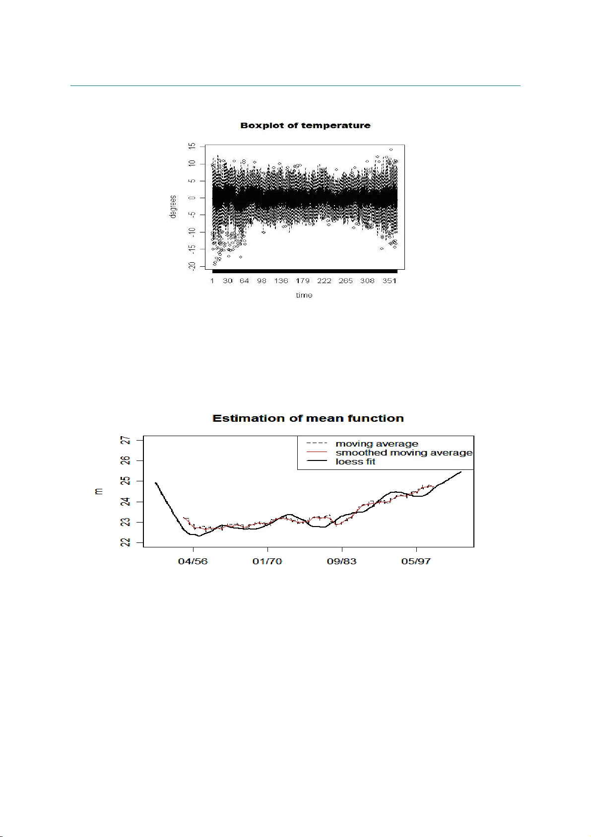
Estimation of a diffusion model with trends taking into account the extremes. A ppl ication to temperature in F rance [1] Laboratoire de Mathématiques, Université Paris 11, Orsay, France [2] Gaz de France Research and Development Division, Statistics and Artificial Intelligence Section ! SUMMAR Y . W e built a model of the daily temperature based on a diffusion process and address to extreme values not taken in account into the literature on this kind of models. We first study, using non parametric tools, t he trends on mean and variance. In a second step we estimate a stationar y model first non parametr ically and t hen using likelihood methods. Extreme values are taken into account in the estimation of model and to obtain a definitive estimation we use in a specific f ramework extreme theory for diffusions. A test of suitable model by simulation is done. Key words: statistics, diffusion process, extreme values, inaccessible boundary, simulation. INTRODUCTION We would like to address the construction and est imation of diffusion m odels in a simulation perspective. Discrete m odels linked to diffusions probably remain until to day the best class of processes describing the daily temperat ure. They allow to compute by simulation the probability of some complicated events, often linked with the behavior of t he diffusion process over high (low) thresholds. Recently, two fields have been more directly concerned with this problem: climate and f inance, and often the t wo fields are concerned jointly with energy prices. This paper is dedicated to a specific point: estimate and test a suitable m odel taking in account extreme values. Then apply the model to the daily temperature in France. The starting point of the literature is a discret isation of an Ornst ein-Uhlenbeck pr ocess using an Euler first order scheme, with a seasonal deterministic component, leading to the so- called Vacisek’ s model given by ( ) , ) ( ) ( ) ( t t t dW t dt X t t d dX σ β α β + − + = (1) where β and σ are det erministic seasonal components for the drift and the diffusion coefficient r espectively, α allows the return to equilibrium for this st ationary diff usion, W is a Brownian motion. The discrete version is ( ) ( ) , 1 1 1 n n n n n n X X ε σ α β β + − − = − − − (2) where ε n is a standard Gaussian white noise. Since these first works, (see Dornier et al. [15] f or instance), some modifications or improvements have be done, (see Alaton et al. [2]). Brody et al. [ 7] argue for choosing a fractional Brownian motion in (1) instead of a Br ownian motion, justified by long memory behavior but without statistical evidences. Benth et al. [3] take a Levy process (with a pure jump component) instead of the Brownian mot ion and work with hyperbolic distributions. Campbell et al. [8] propose important changes starting from t he discrete version (2) where α X n-1 is replaced by ∑ − k l n l X 1 α (the statistical procedure lead to k = 3) , so a longer memory and secondly ε n is no more a w hite noise but a GARCH process , 2 2 1 2 1 2 n n n n η β η ε γ ε + = − − where η is a Gaussian white noise. We don’t discuss here ARMA or more generally classical t ime series m odels, see Roustand [28], Moreno et al. [ 22] and Cao et al. [9] since they do not seem adapted to our problematic. All these models take into account only what we call the “central part” component of the whole dat a when t hey test the quality of simulations, in fact they do not look to the extreme values, for instance the y work only on quantile empirical intervals like ( q α , q 1- α ) , with α = 5/100. Nothing is said about t he quality of the model f or tails and in our specific application for very high (or low) temperatures. The previous models and mor e specifically the Vacisek’ s type one given by (1) has a good behavior in the central part when it is estimated using a learning period of observation of 50 years keeping one data per day to fix the ideas. But as we shall see in Part 1, it doesn’t represent the extreme part, being to hot in winter and in summer. It is clear from a statistical study that there are various reasons to such an unsatisfactory behavior of the model (1). The main r eason lies in the choice of a diffusion coefficient which does not depend on the state X t . As a consequence, they have let completely out the study of t he extreme part values, for instance if the diff usion is st ationary with an inaccessible boundaries r 1 ,r 2 , t hey do not consider the question: are r 1 , r 2 finite infinite; specific features on the estimated density of t ransition prove t he inadequacy of models directly associated with an Ornstein- Uhlenbeck process. Other basic problems are seasonality and non st ationarity, and specifically trends produced in our example by an anthropic effect . I t results from some works (see for instance Nogaj et al [24], Parey et al [26]) that t he trends are not t he same in extremes and in the central part, these trends are difficult t o capture in t he com plete model. W hat is clear from the box plot data (see figure 6.1) is that the variability depends of course of time (seasonality) but also of state (temperature). For instance it increases st rongly for low temperatures, physical evidence implies annual seasonality. So it is always easy t o separate state and time effect for very low temperatures. In order to split t he technical problems, this first will address only pr oblems which do not need a study of seasonality so we have divided our work into two papers. In the first one, centered on t he general problematic, we will st udy data which is homogeneous with r espect to the seasonality as f or instance t he data provided in winter. In a second paper centered on seasonality, we work on the whole data set which is more relevant for the applied results as it treats a much larger amount of data. Also some practical problems are induced in this first part for it remains some seasonality effects even in the chosen quite homogeneous seasons. We start with a model , ) , ( ) , ( t t t t dW t X dt t X b dX σ + = (2’) We choose a particular case non depending direct ly on t : . ) ( ) ( 1 t t t t t Z a Z b Z Z ε + = − + (2’’) where Z t is centered and normalized variable of X t : ) ( ) ( t s t m X Z n t − = and m(t) and s(t) being respectively the mean and t he variance tr end. We discuss also the proper definition of trends. We study the extremes of the process using the classical G EV theor y. G EV theory gives useful arguments to choose the values of the inaccessible boundar y ( r 1 , r 2 ) of t he diffusion, r 1 can be taken as the lower bound of the distribution of X t . Probability theory results (see Berman[5] and Davis[14]) allow to link GEV theory and the values of the drift and diffusion coefficients. It seems that the use of these tools is new in st atistic and w e have to make some weak hypothesis in order to built a bridge, convenient for a statistical use between extreme paramet ers est imation and diffusion coefficients ones. T o estimate the model we follow these steps : 1-we estimate the trends m(t) and s(t) 2-Then we work with Z centered and normalized, ) ( ) ( t s t m X Z n t − = 3-we estimate the values of the boundary of t he diff usion and also the behavior of the drift b and the diffusion coefficient a near these boundary values 4-we use non parametric methods for a first estimat e of b and a 5- we choose a two piecewise polynomial parametric model for b and a submitted to adaptative (estimated) constraints given by the first step: a has to be zero at t he boundary and extreme theory f ixes the slope of a at the same boundary. W e also need to choose from data a specify value of first derivative of a at the break point. Under these const raints; the first polynomial of the is estimated using m aximum likelihood, with a plug- in method, the other one is fixed by the constraints An other way could be to use an approximated likelihood with respect to t he size of the lag of discretization as introduced by one of the authors (Dacunha-Castelle et al [13]) and improved by Ait-Sahalia[1]. Computations are ver y heavy and so we do not use these ideas. The series consist of 3-hours daily minimal temperature of about 50 years. We only work with the daily maximum in the hot season . So with respect to the diffusion, there is a met hod of measurement: maximization (minimization) and a discretisation. W e don’t discuss in this paper t he ef fect of t his t wo simultaneous operat ions (from theoret ical point of view see Dacunha et al [13]) .We don’t discuss the use of refined discretisation scheme, this point has to be treated in another work (see Talay [31]). Of course these problems are as important for extremes as for the centr al part for the lag of discretization plays a ver y important role (see Pitterbag[27]) for a discussion of this pr oblem in the case of Gaussian processes). The paper is organized as follows. In t he second part we will estimate t he mean trend and the scale trend of the series by the non parametric method. Part III is devoted to extreme theory. Pract ical procedures are proposes t o include the results of extreme theory in the construction of t he diffusion model. Part IV is devoted t o the estimation of drift and diff usion coefficients. Non parametric and parametric methods are used and discussed. Part V and VI will be dedicated t o simulation procedure. W e test the validity and adequacy of the model using the simulation. To do that we w ill com pare the estimates obtained from observat ion and from simulation for: densities (marginal and conditional), dr ift and diffusion coefficient, clusters length (defined as the number of consecutive days where t he t emperatures are larger (smaller) than a given threshold), GEV parameters. Finally in Part VII w ill be a discussion and will present some perspectives. " 1. ESTIMATION OF MEAN FUNCTION AND SCALE FUNCTION The mean m and the scale s are the function of t (the dates) ; they describe the behaviour of the t emperature X for a large scale of t ime . The the drift and diffusion coefficients describe the variations of the temperature for a short scale of t ime. From a practical point of view and to check t he trends effects, If we don’t take account of the mean trend m(t) and scale trend s(t), that means we consider m(t) and s(t) as a constant, we have the formula: n n n n n X a X b X X ε ) ( ) ( 1 + + = + (3’) If only m is taken account, then we have: n n n n n Y a Y b Y Y ε ) ( ) ( 1 + + = + (3’’) ) ( n m X Y n n − = . If both of m and s are taken account: we come back to the formula ( 3). In this section, we discuss the method t o estimate m and s . Moving average is often used to estimate the mean m . W e have chosen as a non parametric method LOESS, or locally weighted scatterplot smoothing because of its intuitiveness and simplicity. This method has advantages to deal with the moving average. LOESS combines much of the simplicity of linear least squares regression with the flexibility of nonlinear regression. The fit at x is made using points in a neighbourhood of x , weighted by their distance to x . Throughout this paper, we use LOESS with a local polynomial of degree 1 (linear local smoothing). The m oving average gives a same weight to all points in the localized subsets, so part of the variation in the data is ignored. Let look at the figure 6. 2 which describes the mean function estimator for t he hot t emperature. W ith a moving window of 1049 da ys, the estimat or by LOESS has a similar behaviour than the estimator by moving average with a moving window of 501 days while t he estimat or of moving average with a window of 1049 days makes disappear some peak values. Boundary effects are w ell-kno wn in nonpa ramet ric methods; they a ffect the g lobal performance and also the rate of convergence in the usual asymptotic analysis. The study of Ming-Yen Cheng and al [11] (1997) about the boundary effect in LOESS showed that a good solution to improve the estimation at the endpoints is just to apply the triangular weight kernel ) ( ) 1 ( ) ( ] 1 , 0 [ u I u u K − = . I n fact, f or our data, even without this correction, the boundary effects of LOESS estimators don’t create lot of troubles (see figure 6.2, 3). The problem of robustness is antagonist to the use of inform ation coming from extremes. Nevertheless, from a practical goal, we study t he r obustness for m. Cleveland [12] ( 1979) proposed a robust estimation procedure f or LOESS by using Tukey’ s biw eight. W e can check the robustness of mean function m by this method. We remove respectively 1% to 5% of higher and lower values of the sample data and with each robust sam ple, we estimate m by LOESS and robust correction like above. W e find that when we remove step by step extreme values, the mean behaviour doesn’t change; they have the corresponding peak values at the same t ime; but t here exists a constant distance bet ween the estimator s. So we use a very moderate 1% estimate. . T he smoothing parameter controls the smoothness and t herefore has a crucial influence on the inference about m . T here are several methodologies for automatic smoothing parameter as differ ent cross-validation. But these criteria valid f or i.i.d. data are t oo sensible to dependence to be use f or our data without precaution. So we have to use often selection like rules of t humb or the minimization of the global for prediction to select a suitable parameter which allows to obtain a bias and variance trade-of f. # Variance f unction estimation in regression is more typically based on the squared residuals from a preliminary estimator of the mean function. After estimating mean trend m , we can estimate the scale function when we consider s like the mean function of square residuals regression. So the estimator of s has a f orm: ∑ − = i i i i x m X x w x s ))² ( ˆ )( ( ) ²( where w is t he chosen weight function. Recently Ruppert [29] used the linear local regression for variance estimation; the influence of est imator of t he mean function and t he selection of bandwidth is also discussed. Ruppert has shown t hat the leading bias and variance term for our local polynomial var iance estimat ion ar e analogous to t hose for local polynomial est imator of the mean function; so that there is no loss in asymptotic efficiency due t o est imating m . Ruppert proposed the same bandwidth selection for both of estimations of mean funct ion and scale function. 2. EXTREME THEORY IN DIFFUSION PR OCESS In order to apply G EV t heory to diffusions, let us state some results from probability theory. The first one concerns the maximum on an interval for a stationary diffusion when the length of the interval increases. T he basic results are due to Berman [ 5] but the version of Davis [14] fits a statistical framework better. First, we are concerned by a stationary diff usion with invariant densit y ν and inaccessible boundaries i r and s r which are finite or infinite but unaccessible ( Breiman [6]). Let a diffusion X with liptchitzian coefficients a and b defined by : t t t t dW X a dt X b dX ) ( ) ( + = the scale function s of the diffusion ( ) is given by ∫ ∫ = − x dv v a v b du e s u ) ( ) ( 2 2 1 (we keep t he traditional notation s for t here is no possible confusion in the paper with t he trend s of the variance) Theorem If M T = max(X t ), 0 < t < T, if it exists f unctions A and B such t hat T T T A B M − converges in distribution to G, then G is a GEV distribution define in the following manner : if F is the distribution defined by then F is in the (extreme) domain of attract ion of G. Remark : This m eans that the G EV distribution G associated to the max value in a large block of consecutive observations at discrete t imes is not in general t he same GEV distribution H associated to a sample of the marginal density ν . It can success that the domain of attraction of H is different of G even for instance with diff erent shape parameters ( see Davis (9) for an example ). Application : we can see from the previous theorem that F has particular properties : as a and b are continuous on the interval (r I , r S ) (and even in general supposed liptchizian) functions with a>0 we see that F is twice continuously different iable, so t he formula giving F shows that ' ' ' ) log( 2 1 ' 2 ' ' ' F F F F F a b s s + + − = − = (**) $ from s t ends to infinity as X t ends to r I or r S , and in this case a t ends to 0 . Suppose that F is in t he domain of max-attraction for some GEV distribution G with shape parameter ξ<0. We now from the general theory of extremes (Embrechts et al[17]) that this means that as x tends to r S , we have 1- F( x ) equivalent to L( x ) x -1/ξ so this means first that t he upper bound of g is r S and that 1/ s is equivalent to L( x ) x -1/ξ as x tends to r S . Definition We say that a C 2 -function f with regular variation is of C 2 -regular variation as x tends t o r S if for some ξ, we have f ”(x) equivalent t o x ξ L(x) with L of slow variation as x tends to r S . For instance, if 1-F(x) is equivalent t o to x ξ L(x) with L is a function product of different powers of iterated from different orders logarithms then 1-F(x) is of C 2 -regular variation. From a statist ical point of view, it is well known t h at it is very difficult (quite impossible!) to estimate L when ξ is unknown and even if it is known ( as it is very difficult t o know if F is in a max domain of attract ion). So to suppose for a t wice differentiable function t hat it has t he C 2 - property of regular variation it is not in practice restrictive with respect to the hypothesis”it belongs to a max-domain of attraction”. So we can obtain the following lemma: Lemma : Suppose F of C 2 -regular variation and in the domain of at traction (for maximum) of ) , , ( ξ σ µ G , 0 < ξ , let r S the common upper bound of F and G. Then we have the previous behaviour (**) for F as X t ends to r S , t his result is independent of the slowly varying function L (which can be of course constant) We have the following behavior of a near the upper bound s r , ) 1 1 )( )( ( 2 ) ( − − − − ≈ ξ x r x b x a s This lemma thus proves that if two diffusions have the same drift and the same 0 < ξ and the same upper bound then necessarily near t his bound the diff usion coeff icient are equivalent to the same linear form, in fact they are linear up to the first order and are also t he same for every ) , ( σ µ such that ξ σ µ − = S r as ξ are fixed. Proof : from F’’(x) %& ' ) 2 1 ( ) ( − − ξ x x L we deduce by integr ation the equivalences for F’ and log F and apply the formula (1). So we now have an est imate a ˆ by t he plug in method of a near the bounds if, 0 < ξ f or t he two bounds, ) 1 )( ˆ )( ( ˆ 2 ˆ ξ − − − = x r x b a s We only consider this case 0 < ξ here, for temperatures in France have negative ξ . " ESTIMATION OF THE DRIFT AND THE DIFFUSION COEFFICIENT Estimation of the diffusion process or stochastic differential equation has been considered in the literature for many years, with some the papers being concerned with estimating the drift and diffusion f unctions from continuously sampled data. However with discretel y sampled observations from the continuous sam pling path, estimation of the continuous-time diffusion process is more complicated and mor e if one has to discuss the role of the lag for ( discretization. W e work with nonparametric estimates first and then with parametric estimates for the drift and diffusion coefficient. The first parametric estimator of the coefficients of a stationary diffusion process fr om discretely sampled observations taking in account the lag is the approximate maximum likelihood estimator proposed by Dacunha-Castelle and al [13] (1986). T his result was improved by Ait- Sahalia[1]. Other parametric estimators include the maximum likelihood estimators derived by Lo [20](1988) for more general jump-diffusion processes, the method of moments based on simulated sampling paths f rom given parameter values proposed by Duffie and Singleton [16](1993). Many authors [30](1997) used kernel regression or wavelets for instance to construct nonparamet ric estimates for the diffusion coefficients . We first est imate b in the supplied model by local smoothing LOESS where b is considered as t he conditional expectation E(Z n -Z n-1 |Z n-1 ). The behavior of b ˆ in the central part from 1%- quantile to 99%- quantile is rather linear. Local estimation in 1% higher and lower value, because of lack of observations, seems to have no physical and probably statistical meaning using this method. Besides, when considering b like a polynomial and using likelihood tests, we can find out a polynomial of degree 1 is the optimal model for b . Comparing local estimator b ˆ with linear least squares estimator of b , we f ind that they merge in the central part (see figure 6.3). In summary, we can consider b as linear. A study on t he robustness of b is necessar y. It comes back to the same idea in t he previous section: that is to r emove respectively 1%, 2%, …, 5% higher and lower of the sample and observe how the drift estimator changes in the central part. T he linearity of b follows acceptable by likelihood tests. We obtain always a negative linear drift but more t he values in extreme parts ar e removed, steeper is t he slope of the drift. For example, with a stationary diffusion m odel for the cold season, from a slope of drift β = -0.22 with nothing removed, we have a slope β =-0.29 with 5% higher and lower values removed. This gap is rather large. W e know that the estimators by least squares are not robust. I ndeed this change is more clearly seen for cold temperatur e. The cold temperature is less homogenous than the hot temperature ( see figure 6.1). For this reason, if we use a robust b , it improves the results in the central part but gives a bad estimat ion for high quantiles For we are interested in extreme values, we don’t use robust estimator; we keep all the observations sequence for estimating b. To estimate a , we can consider it as the square root of the conditional variance function of Z n given Z n-1 . We estimat e it using a kernel method. If K is a kernel (Epanichkov or Gaussian are used) and h is the corresponding bandwidth then the conditional density is estimate as − − − − = − = ∑ ∑ n n N n N n n N n n n N h y Z K h h y Z K h x Z K h 1 1 1 1 2 1 1 and its mean and var iance as usually directly, the summand in the numerator being multiplied by an adequate term. Then, we compare the results with the estimate obtained f rom a penalized likelihood method . We start from the density ) − − − − − − − 2 1 1 1 1 ) ( ) ( 2 1 exp ) ( 1 n n n n n Z a Z b Z Z Z a So the penalised likelihood is given dx x a Z a Z a Z b Z Z a n L n i i i i i i )]² ( " [ 2 1 ) ( log ) ( ) ( ˆ 2 1 ) , ( 2 1 2 1 1 1 ∫ ∑ − − − − − = = − − − − λ (4) with a convenient regularization parameter λ , where b ˆ is estimated by linear least-squares: 1 1 ) ( ˆ − − + = n n Z Z b β α as previously. T he maximization of l gives a as a cubic spline function. This is the first step. A recursive procedure checks the stability of est imation of a and b . T hat means with a ˆ estimated from (4) ( called original a ˆ ), we estimate a new linear b by maximizing: ∑ = − − − − − − − − n i i i i i i Z a Z a Z b Z Z 2 1 2 1 1 1 ) ( ˆ log ) ( ˆ ) ( 2 1 and we resume. The result of these work it erations give us the same estimators of a and b. In deed, we can also estimate a and b at the same time by (4), this is theoretically possible but the numeric implementation takes too much of time. We pass now to a parametric estimation, the parametric model is suggested by all the previous results, the one on extremes and t he non parametric estimates We estimate a and b at t he same time first by considering a as a polynomial p (of degree 4 in our case): ∑ = n 2 i 1 - n 2 1 - i 1 - n 1 - i i ) p(Z log - ) p(Z ) b(Z - Z - Z 2 1 - (4’) So after maximizing (4’), we obtain estimators of parameters: 2 for b and 5 for a . We can compare the behavior of a ˆ obtained b y parametric and non parametric met hods. Near the boundary,say1% higher and lower values of X , estimators of a and b have not sense for there are not enough date to perform directly any estimat e and so we have to use extreme t heory to make a kind of extrapolation. So the comparison excludes this neighborhood of the boundary. The parametric est imator of a in (4’) is retained for implementation. With these parametric estimators of a and b , we obtain the residuals which can be tested. T hey are accepted as a white noise aft er considering their first and second moments, their autocorrelation plot and qq-norm plot. Next a same work to b is realized for checking the robustness of a . But in this case, we focus more on the extreme part. W e remove just respectively 1% to 3% of lower values. From the three robust samples, we consider the difference of the estimated a from robust samples with one of original sequence: ∑ − = ∆ i Y i X Y X , , ) , ( θ θ with θ the coefficients of polynomial of 4 degree, estimator of a. We obtain the values of ∆ of 3 robust samples with the whole series respectively: 0.021, 0.027 and 0.05. The third one(-3%) has different behavior of a ˆ in some parts. In the first one (-1%) and the second one (-2%), the diff erence can be acceptable. We propose now to separate the estimation of a and b in the central part (from 1%-quantile to 99%-quantile) and extreme part (from 1% to the boundary): a cent and b are estimated by all of the observations. T hen a in the extreme part (>99% and <1%) is estimated differently. * The drift function has a quite clear physical meaning as the elastic part of the basic oscillator which the deterministic justification of the Ornstein –Uhlenbeck first model. So we suppose that this drift is valid until the boundary and we discuss later this hypothesis. When applying GEV distribution for the maxima (respectively minima) of our series of temperature in France, usually we obtain ξ <0, which means the temperature is bounded. And their upper bound (r espectively lower bound) can be estimated from a function of the estimators of extreme parameters of GEV distribution: ξ σ µ − = S r Testing t he quality of the estimators of a and b in formula (4’) by simulation, we can see t hat the simulation-based empirical quantiles (from 1000 samples) in the central part (from 5% to 95% quant ile) are really close to the tr ue quantiles : a maximal difference of 0.5°C is found. However in the tail, (from 1% to 3%) we find out a difference of about 1.5°C. This bias in climatology is rather large even if we take into account that the record observed on 1000 samples is much larger than the observed one and so this has an influence on the 1% quantile. , In summar y, simulated t ails are heavy than the observed quantile as a simple consequence of t he law of large numbers. It remains to give a more precise definition of “where the tail begins” in the whole distribution. We need a correction for the diffusion coefficient a in the tail. Our idea is based on a theoretical r esult, t he behavior of a at the boundary In the pr evious section, we have applied GEV distribution f or the extreme values of diffusion process and we obtained a parabolic form in the neighborhood of the boundary (see lemma, part 3). T here is not any assurance that this is well modeled for all “ extreme” par t. So for another part we look for a suitable experimental estimator of a for 1% higher and lower values. Thus the lack of theoretical results obliges to use an interpolation in order to complete the function a ˆ . We look for here a suitable polynomial of degree 2 (to follow to the extremes theory) which satisfies t he condition at the boundary (a(r S ) =0) and t wo another constraints are added t hat a ext (q 0.01 )=a cent (q 0.01 ) and a’ ext (q 0.01 ) given b y t he lemma. In another tail, higher than 99%-quantile for the cold temperature, do we need a correction of a? The high values in daily minimum temperature in t he winter are not really homogenous and in fact t heir role is not really important, we can use a cent for this part. Remark: These estimators are then built by a plug-in method from the estimators given by GEV estimates and by an empirical quantile, t he remaining is provided by the likelihood method. So it can be show that the estimators of a and b are consistent, with a speed of convergence n / 1 , the computation of t he matrix of information is very complicated and details will be given elsewhere. 4. SIMULATION AND RESULTS We simulate 3 models: 1/ m and s are considered as constant: 2/ m is a function of time and s is constant 3/ both of m and s are functions of t ime. In order to validate a suitable model for our data, we make 1000 simulations basing on the models above for the low temperature. To test the quality of the model, we have to determine whether the simulation model is an accurate representation of the observations. T he comparison is based on the following items: Quantiles + Marginal density, mode, mean, variance GEV estimated distribution and its paramet ers Clusters distribution: number of clusters and length for observation less than the threshold given by quantiles 1% and 2% and larger than threshold given by quant iles 98% and 99% The simulation procedure: MODEL 1: • Estimate a and b from the initial sequence X with the method described in part 4 • With these estimated a and b , simulate 1000 samples wi t h a recurrence procedure by using n n n n n X a X b X X ε ) ( ) ( 1 + + = + MODEL 2: • Estimate the mean function m of X and calculate Y= X - m • Then use the same procedure as for m odel 1 with Y instead of X • Deduce 1000 samples of X by adding m : X=Y+m MODEL 3: • Estimate the mean function m and scale function s of X , calculate Z=( X - m )/ s • Then use the same procedure as for m odel 1 with Z instead of X • Deduce 1000 samples of X by adding m and multiplying s : X=sZ+m We obtain the results for cold temperature: Quantiles: Below we const ruct a table with the em pirical quantiles cor responding to three kinds of models for the cold temperature. W e consider from 1 st percentile to 99 th percentile, smaller or higher percentiles have not a significant meaning. Let O for observation and S for simulation Percentiles O S without m and s S w ith m S with m and s 1% -14.40 -14.07 -14.96 -16.21 2% -12.44 -11.78 -12.27 -12.74 3% -11.40 -10.43 -10.79 -11.08 5% -9.40 -8.73 -8.98 -9.13 10% -6.60 -6.42 -6.58 -6.64 30% -2.20 -2.49 -2.53 -2.55 50% -0.10 -0.18 -0.19 -0.20 70% 1.90 1.98 1.96 1.95 80% 3.20 3.26 3.23 3.21 90% 5.30 5.08 5.00 4.97 95% 6.80 6.66 6.54 6.50 97% 7.51 7.77 7.61 7.57 , 98% 8.14 8.63 8.46 8.42 99% 9.30 10.11 9.94 9.92 Three cases give us the different results of empirical quantiles, especially in the cold extremes. In the central part from 1 st percentile to 95 th percent ile, we don’t find an important difference between the thr ee models. A difference about 0.1°C is found for the median, but this difference is smaller for the percentile s close to the median. This is not found for the hot temperature but for cold t emperature it is implied by a remaining of seasonality which as w e will show in t he second paper disappears when the whole data is taken in account.. However 0.1 of difference is not really significant. The empirical quantiles for three models can be considered rather good versus the true quantiles. In the extreme part, from 95 th to 99 th percentiles, the third model with m and s seems a little better than other ones. For 1% and 2% quantiles, the third model seems bett er with the difference larger for the smaller percentiles, while which is inverse for two other ones. In the case of hot temperature, it is surprising that the results in 1 st model and 2 nd model with mean trend are mostly analogous. m in summer has a total variability of 3°C, t hat means that m cannot be considered as constant. T he diffusion cannot be considered as stationary. Indeed, observing two m odels: stationary and st ationary with a mean t rend, we can see that when m is difference-stationary ( ∆ m is stationary) with zero mean, b’(X-m) plays the role of mean function of ∆ X , so it is identical with b ( X ). From the same argument, we have a(X)=a’(X-m) , where b, b’ and a, a’ ar e respectively drift functions and diffusion f unctions of stationary and non-stationary diffusion process. Hot temperature has a linear tr end for t he mean. W ith a ADF test, we can check it. In the figure 6.5, we can find out the similarity of a and b in t wo models. No difference can be seen between the empirical quantiles because the quantiles don’t pay attention to t he order of values. Marginal density: The simulations of all three models have a median and mean near by t he true median and true mean. However their variance is smaller; their values are m ore concentr ated near t he mode which is also the median. W e already explain this defect by the remaining seasonality Estimators of GEV parameters With our modelling in the tail of a , the empirical estimators of GEV parameters are rather good (see figure 6.5). T he mean of the simulated location parameter µ approaches the true µ . The scale paramet er σ is not so well estimated for the hot temper ature because the simulations can catch of t he strong variability of the extreme hot temperat ure in the last years. The shape paramet er ξ is difficult to estimate, but in our case, t he simulated empirical estimation of ξ is very good. Clusters We concentrat e on the rate of declusterization (which is can be considered as t he inversion of average length of the clusters) and the distribution of clusters. For hot temperature, the average length of clusters of simulations is smaller than t he observations one. The distribution in the 2 nd simulated model ( wi th m ) seems to be nearest to that of observations. For cold temperature, the results of the 3 models are rather similar. 5. GRAPHICS 5.1 Data estimations Box plot of data without seasonal component for the mean shows the seasonality of the mean and of the variance, this one is ver y large in W inter and the marginal densities are asymmetric 5.2 Adv ant age of LO ESS method versus moving average: The mean trend estimators by moving average and LOESS with a window of 1049 days (correspond to 11 years) 5.3 Estimation of drift function b estimated for the sequence of temperature in cold season in Strasbourg b estimated by LOESS approach b estimated by linear least square in the central part (which is limited by the vertical lines) 5.4 Estimation of diffusion coefficient a Different estimations of a in the central part : non parametric and parametric The oscillations are not significative (lack of data) for very low temperatures " Estimation of a in the central part and extreme part which is separated by the dash- line of the 1 st percentile $$ Simulation 1000 samples of simulation for the diff usion equation. Diffusion coefficients Comparison between a( X ), b ( X ) in 1 st model and a’( X - m ), b ’( X - m ) in 2 nd model with mean trend: they are mostly coinciding # Marginal density Marginal density of the observations and the simulations The effect of seasonality remains in the simulated model of t he winter (3 months). It implies that the variance of the simulations is smaller than that of observations. T his fact is not found in the simulated model for just one month (January) but a clear difference is found in the cold extreme part because of the lack of values . GEV parameters Estimation of GEV parameters in the simulations The vertical lines are the true parameters with t heir confidence intervals of 90% $ Clusters Hot temperature O S 1 st model S 2 nd model S 3 th model Quantile 98% Threshold 32.80 33.15 33.11 33.19 Length 1 2 3 4 5 6 7 Distribution 0.700 0.150 0.050 0.033 Distribution 0.695 0.202 0.070 0.022 0.007 0.003 0.001 Distribution 0.715 0.193 0.061 0.020 0.007 0.003 0.001 Distribution 0.703 0.195 0.065 0.024 0.008 0.003 0.001 Rate of declusteriza tion 0.588 0.686 0.703 0.686 Quantile 99% Threshold 34.00 34.47 34.43 34.60 Clusters Length 1 2 3 4 5 6 Distribution 0.824 0.059 0.088 0 Distribution 0.776 0.174 0.039 0.009 0.001 Distribution 0.807 0.148 0.033 0.009 0.003 0.001 Distribution 0.778 0.161 0.043 0.013 0.004 0.001 Rate of declusteriza tio 0.654 0.777 0.796 0.764 Cold temperature O S 1 st model S 2 nd model S 3 th model Quantile 2% Threshold -12.44 -11.77 -11.77 -11.76 Clusters Length 1 2 3 4 5 6 7 8 Distribution 0.478 0.283 0.065 0.022 0.043 0.022 0 0 Distribution 0.564 0.203 0.099 0.053 0.032 0.018 0.011 0.007 Distribution 0.568 0.205 0.097 0.054 0.030 0.018 0.011 0.007 Distribution 0.571 0.201 0.098 0.053 0.032 0.019 0.011 0.007 ( 9 10 11 12 13 0.022 0.005 0.003 0.002 0.001 0.001 0.004 0.003 0.002 0.001 0.001 0.004 0.002 0.001 0.001 Rate of delusterizati on 0.447 0.497 0.505 0.505 Quantile 1% Threshold -14.4 -14.07 -13.98 -13.97 Clusters Length 1 2 3 4 5 6 7 8 9 10 11 12 Distribution 0.600 0.167 0.200 0 0.033 Distribution 0.588 0.204 0.098 0.049 0.027 0.015 0.008 0.005 0.003 0.001 0.001 0.001 Distribution 0.597 0.206 0.093 0.047 0.026 0.013 0.008 0.004 0.003 0.001 0.001 Distribution 0.599 0.201 0.095 0.049 0.026 0.013 0.008 0.004 0.002 0.001 Rate of declusteriza tio 0.588 0.535 0.547 0.546 CONCLUSIONS AND PERSPECTIVES Our pur pose is to find out a parametric diffusion. We choose the m odel which takes in account the mean trend and scale trend. T he most interesting result is that t he modification of the diffusion coefficient now highly non linear as a function of the temperature gives a model of simulation with the following properties: 1- It keeps the qualities of the classical seasonal model based on O rnstein-Uhlenbeck model for data in the central part 2- At the opposite of the classical model, it gives a good fit t o t he dat a ( observed quantile q) for 2%
Original Paper
Loading high-quality paper...
Comments & Academic Discussion
Loading comments...
Leave a Comment