Fuzzy sets in nonparametric Bayes regression

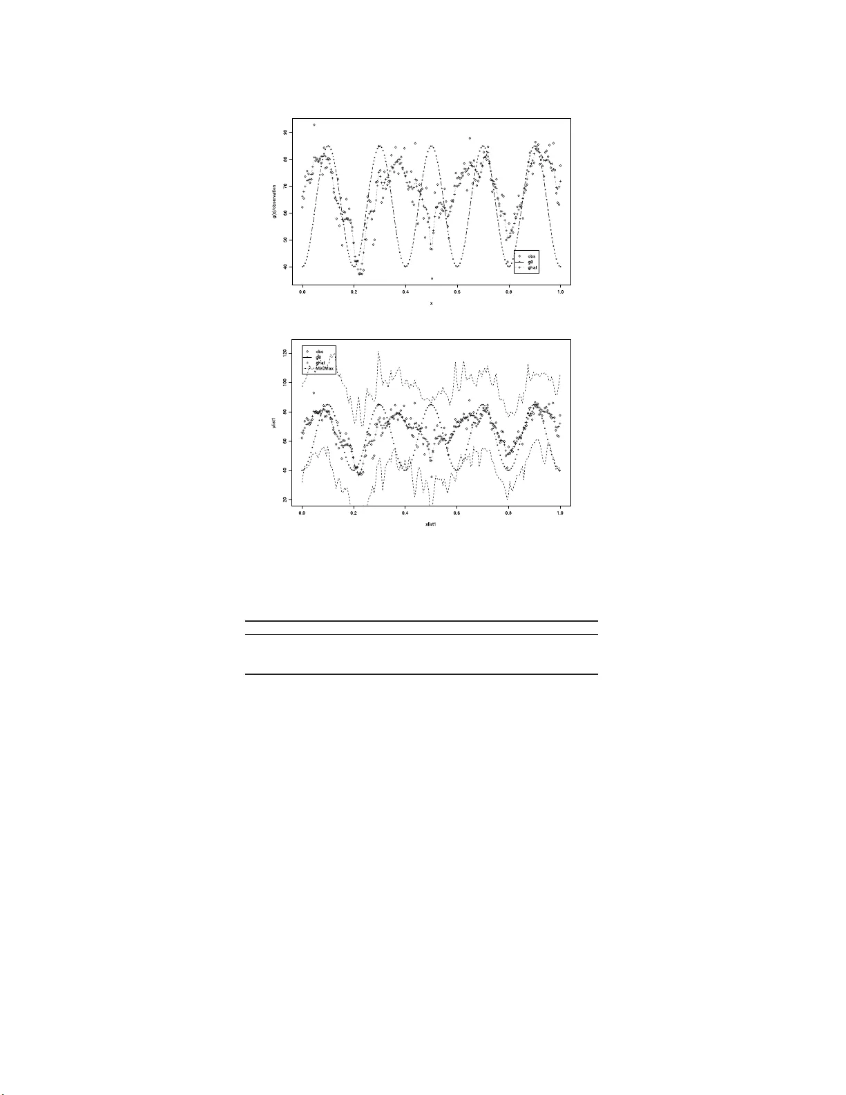
IMS Collectio ns Pushing the Limits of Con temp orary Statist ics: Contributions in Honor of Jay an ta K. Ghosh V ol. 3 ( 2008) 89–104 c  Institute of Mathe matical Statistics , 2008 DOI: 10.1214/ 07492170 80000000 84 F uzzy sets in nonparametric Ba y es regress ion Jean-F ran¸ cois Angers 1 and Mohan Delampady 2 Universit´ e de M ontr ´ eal and Indian Statistic al Institute, Bangalor e Abstract: A simple Bay esian approach to nonparametric regression is de- scrib ed using fuzzy sets and membership functions. Membership functions are int erpreted as likelihoo d functions for the unkno wn r egression function, so that with the help of a reference prior they can be transf ormed to prior den- sity functions. The unkno wn regressi on function i s decomposed into wa velets and a hierarchica l Bay esian approach is empl oy ed f or making inferences on the resulting w a v elet coefficient s. Con ten ts 1 Int ro duction . . . . . . . . . . . . . . . . . . . . . . . . . . . . . . . . . . . 89 2 Nonparametric regr ession a nd wa v elets . . . . . . . . . . . . . . . . . . . . 91 3 Prior information and members hip functions . . . . . . . . . . . . . . . . 92 4 Posterior calcula tions . . . . . . . . . . . . . . . . . . . . . . . . . . . . . 9 4 5 Mo del chec king and Bayes factors . . . . . . . . . . . . . . . . . . . . . . . 9 7 5.1 Pr ior robustness of Bayes facto rs . . . . . . . . . . . . . . . . . . . . 9 8 6 Examples, simulations a nd illustrations . . . . . . . . . . . . . . . . . . . 100 6.1 Mo del chec king . . . . . . . . . . . . . . . . . . . . . . . . . . . . . . 1 02 7 Conclusions . . . . . . . . . . . . . . . . . . . . . . . . . . . . . . . . . . . 1 03 Ac knowledgmen ts. . . . . . . . . . . . . . . . . . . . . . . . . . . . . . . . . . 104 References . . . . . . . . . . . . . . . . . . . . . . . . . . . . . . . . . . . . . . 1 04 1. In tro duction Consider the mo del (1.1) y i = g ( x i ) + ε i , i = 1 , . . . , n, and x i ∈ T , where ε = ( ε 1 , ε 2 , . . . , ε n ) ′ ∼ N (0 , σ 2 I ), σ 2 is unknown and g ( · ) is a function de fined on some index set T ⊂ R 1 . Inferences ab out g such a s its estimation and es tima tio n error as well a s mo del chec king ar e of in terest. Without par ametric a s sumptions such as thos e leading to linear reg ression, this is a no npa rametric regr ession problem. A Bayesian appr oach to (fully) nonparametric 1 D´ epartemen t de math´ ematiques et de statistique, U nive rsit´ e de Montr ´ eal, M on tr ´ eal H3C 3J7, Canada, e-mail: angers@d ms.umont real.ca 2 Statistics and Mathematics Unit, Indian Statistical In stitute, Bangalore 560 059, India, e-mail: mohan@is ibang.ac .in AMS 2000 subje c t classific ations: Pr imary 62G08; secondary 62A15, 62F15. Keywor ds and phr ases: function estimation, hierarchical Ba y es, membership function, model c hoice, wa velet. 89 90 J.-F. Angers and M. Delamp ady regres s ion problems t ypically requires spec ifying pr ior distributions on function spaces whic h is rather difficult to handle. The extent of the complexity of this approach can be gauged from sources suc h as Ghosh and Ramamoo rthi [ 9 ], Lenk [ 10 ], a nd so on. F ur thermore, quantifying useful prior informatio n such as “ g is close to (a sp ecified function) g 0 ” is difficult pro babilistically , whereas this se ems quite stra ightforw ard if instead an a ppropria te metric o n the concerned function space is used. This is where fuzzy sets or member ship functions can be made use of. Before pr o ceeding to this pro blem, let us reca ll the following details on fuzzy sets and membership f unctions. Definition 1.1. A fuzzy subset A of a space G (or just a fuzzy set A ) is defined by a member ship function h A : G − → [0 , 1]. The mem ber ship function, h A ( g ), is supp ose d to express the degree o f compati- bilit y of g with A . F or example, if G is the r eal line and A is the set o f po ints “close to 0 ”, then h A (0) = 1 indicates that 0 is cer tainly included in A , but h A ( . 05) = . 01 says that .05 is not really “clo se” to 0 in this c o ntext. Similarly , if G is a se t of functions and A ⊂ G is a set of functions “close” to a given function g 0 , then h A ( g 0 ) = 1 indicates that g 0 is certainly included in A ; howev er, if h A ( g 1 ) = . 01 with g 1 ( x ) = 10 g 0 ( x ) + 100 then g 1 is not really “ close” to g 0 in this case. Note that even when G = Θ is the pa rameter space , a members hip function h A ( θ ) is not a probability density or mass function defined on Θ, and he nc e canno t b e used to o btain a prior distribution directly . Instea d, as we hav e done in [ 4 ], we prop ose that a reasonable in terpretation for a fuzzy subset A o f Θ is that it is a likeliho o d function f or θ giv en A . (See also [ 12 , 1 3 ]). This in ter pretation s eems to be able to answer so me of the questions reg arding how a ppropriate the co ncept of fu zziness is in mo deling our p erception of imprecisio n. F r ench [ 7 ] discusses a few of these ques - tions. First of all, likeliho o d is an accepted means for mo deling imprecision. Another impo rtant question is how to define h A ∩ B from h A and h B for incorp ora ting h A and h B in Bay esian inference . If A and B are indep endent, then interpreting h A and h B as lik eliho o d functions leads to the res ult that h A ∩ B = h A h B , for this purpo se. F urther, the qualitative ordering that underlies a mem bers hip function can also b e inv e s tigated with this interpretation, in conjunction with a pr ior distribution, as we study later. See [ 4 ] for an application to hierarchical and r obust Bay es inference. This pap er is closely rela ted to Angers and Delampady [ 3 , 4 ]. In the latter , we used fuzzy sets to help sp ecify a pr ior density on a finite para meter space, wher eas in the for mer a nonpar ametric function estimator using wav elet decomp os ition w as presented. It is therefor e natur al to explore whether a combination of these tw o ideas can b e fruitfully employed. T ow ards this end, we adopt the semi-par ametric approach of using the w av elet decomp os itio n of a regress ion function a long with a r emainder, thus e ffecting a dra stic reduction of the dimension of the parameter space. Next we prop ose to incorp or ate the impre cise prior information o f the k ind “the true r egressio n function g is close to g 0 ” using membership functions. W av elet decomp osition of g 0 provides the w av elet co efficients θ 0 which we take as the prior mean of the wa velet co efficients θ cor resp onding to g . Precisio n o f this prior mea n estimate is unclear, so we trea t the prior v ar iance of these co efficients as a hyper- parameter with a second sta ge (reference) prio r. This appro ach is also tied to the question of Bayesian robustnes s. If a membership function stating “ we think g is close to g 0 ” is the only prior input that we intend to incor p o rate, how sho uld we then pro ceed with the Bay esian inference related to g ? W e claim that the only natural appro ach is to study the ro bustness of the inferences resulting fro m the Nonp ar ametric r e gr e ssion 91 class o f prior densities c ompatible with this mem ber ship function (see Section 5.1). This appro ach is further explained in the following sections. This pa pe r is o rganized as follows. In Sections 2 and 3, a brief s ummary o f our previous work [ 3 , 4 ] is pr e s ented. In Sec tio n 4, details on the pos ter ior ca lculations are given. The main fo c us of this pap er, namely , model c hecking using Bayes factors and fuzzy mo dels, is discusse d in Section 5 . Sim ulations and practical examples are presented in the last section to illustr a te this theme. 2. Nonparametric regressio n and w a v elets T o pro ceed further, we as sume that the regress io n function g and its prior guess g 0 are in L 2 and imp os e a wav elet structure o n bo th of them. T o do this, we consider a co mpactly supp orted wa v elet function ψ ∈ C s , the set of real-v alued functions with contin uous der iv atives up to order s . Thus, g ( x ) can b e written as g ( x ) = X | k |≤ K 0 α k φ k ( x ) + ∞ X j =0 X | k |≤ K j β j,k ψ j,k ( x ) = g J ( x ) + R J ( x ) , where g J ( x ) = X | k |≤ K 0 α k φ k ( x ) + J X j =0 X | k |≤ K j β j,k ψ j,k ( x ) , R J ( x ) = ∞ X j = J +1 X | k |≤ K j β j,k ψ j,k ( x ) , (2.1) φ k ( x ) = φ ( x − k ) , ψ j,k ( x ) = 2 j / 2 ψ (2 j x − k ) , α k = Z T φ ( x − k ) g ( x ) dx and β j,k = Z T 2 j / 2 ψ (2 j x − k ) g ( x ) dx. Here K j is such that φ k ( x ) and ψ j,k ( x ) v a nis h on T whenever | k | > K j , and φ is the scaling function (“father wa velet”) cor resp onding to the “mother wa v elet” ψ . Such K j ’s ex is t (and are finite) since the w av elet function that we hav e chosen has compact supp ort. (See [ 3 ] o r [ 8 ] for details.) Since the num b er of o bs erv a tions is finite, o nly a finite n um ber of parameters c a n b e estimated. Therefore, as suggested in [ 3 ], the r esolution level J should b e chosen such that the total num ber of un- known parameter s which need to b e estimated is no larger than n , the num b er of observ ations. Since the total num b er of α and β parameter s is b ounded by l X 2 J +1 + J ( l ψ + 1) + ( l φ + l ψ + 2) where l X , l ψ and l φ represent the length of the supp or t of T , ψ ( · ) a nd φ ( · ) resp ec- tively , w e r equire this upper b ound to be less than n . The o ptimal resolution lev el J , how ev er, should b e chosen using a Bay esian mo del selection technique, for example [ 3 ]. Consequently , we prop ose that the function g J ( · ) b e estimated from the da ta 92 J.-F. Angers and M. Delamp ady and the function R J ( · ) b e consider ed a s a “ nuisance par ameter” to b e eliminated by integrating it out. F urther we assume that g 0 ( x ) = X | k |≤ K 0 α 0 ,k φ k ( x ) + ∞ X j =0 X | k |≤ K j β 0 ,j,k ψ j,k ( x ) , where α 0 ,k = Z T φ ( x − k ) g 0 ( x ) dx, β 0 ,j,k = Z T 2 j / 2 ψ (2 j x − k ) g 0 ( x ) dx. Since g 0 is given, the wav elet co efficients can b e assumed known. F ro m [ 1 ], it is known that β j,k = O (2 − j s ) where s denotes the degree of “smo oth- ness” of ψ , that is ψ ( · ) ∈ C s ( s > 1 / 2 ). F urther, some of the a priori information wa v elet co e fficient s can be translated into E [ α k ] = α 0 ,k ; E [ β j,k ] = β 0 ,j,k ; (2.2) V ar( α k ) = τ 2 ; V ar( β j,k ) = τ 2 / 2 2 j s ; (2.3) (see [ 3 ] for details). Here , τ 2 is a firs t stag e hyper-par ameter, a suitable prior on which will b e sp ecified later . (It is also supp os ed that E [ β j,k ] = β 0 ,j,k = 0 for j ≥ J + 1.) How ever, the prio r probability distribution on the co efficients α k and β j,k itself will b e sp ecified by a membership function to b e introduced later. Since there are only a finite num ber of β j,k that can be estimated, we cannot exp ect to have a very informa tive pr io r distribution o n the remainder term, R J . How ev er, to b e able to pro ce e d with the Bay e s ian approach, we need to ass ume that R J ( · ) is a sto chastic pr o cess. F or simplicity a nd computatio nal ease, we co nsider a Gaussian pro ces s with zer o mean (compatible with E [ β j,k ] = β 0 ,j,k = 0 for j ≥ J + 1). Spec ific a lly , following [ 3 ], we now as sume that R J ( x ) is a Ga us sian pro cess with mean function 0 and cov aria nce kernel τ 2 Q ( x, y ) where Q ( x, y ) = ∞ X j = J +1 1 2 2 j s X | k |≤ K j ψ j,k ( x ) ψ j,k ( y ) . (2.4) Note that a prior assumption such as β j,k being indep endent normal r andom qua nti- ties will natura lly lead to this prior distribution as can be seen from the Ka rhunen– Lo eve expansion [ 2 ]. W e, howev er, ma ke the stronger assumption that the remainder R J ( · ) itself is a zero- mean Gaussia n but with an unknown prior v ar iance co mp one nt τ 2 . Our r eason for this a ssumption is that, o nce the optimal r esolution level J is chosen using a p ow erful mec hanism such as a Bayes factor , as we suggest later, the wa v elet co efficients at hig her r esolutions are not exp ected to hav e substantial influ- ence o n the wa v elet smo other. Hence R J ( · ) w hich is made up of these higher-order wa v elet co e fficient s will also hav e negligible influence. 3. Prior information and me m b ership functions W e have ex plained in the prev io us s ection that we would like to make use of im- precise pr io r information such as “ g is close to g 0 ” by using a membership function Nonp ar ametric r e gr e ssion 93 which tra ns lates this in to a measure of distance b etw een the co rresp onding wa v elet co efficients. L et us examine the implications o f as s uming that the av ailable prior information is qua nt ified in terms of a membership function (3.1) h A ( g ) = ξ ( ρ ( g , g 0 )) , where ρ is a mea sure o f distance. Due to the wa v elet deco mpo sition ass umed on g as well as g 0 (see Section 2), a na tural choice for ρ is the L 2 distance given by (3.2) ρ 2 ( g , g 0 ) = || g − g 0 || 2 = X ( θ j,k − θ 0 j,k ) 2 , where θ j,k and θ 0 j,k are, resp ectively , the wa velet co efficients of g and g 0 . Using Parsev al’s iden tit y , note that ρ 2 ( g , g 0 ) = k g − g 0 k 2 = X | k |≤ K 0 ( α k − α 0 ,k ) 2 + ∞ X j =0 X | k |≤ K j ( β j,k − β 0 ,j,k ) 2 . Since we canno t estimate β j,k for j = J + 1 , . . . , and b eca use β j,k = O (2 − j s ) (see [ 1 ]) we then have ρ 2 ( g , g 0 ) = X | k |≤ K 0 ( α k − α 0 ,k ) 2 + J X j =0 X | k |≤ K j ( β j,k − β 0 ,j,k ) 2 (3.3) + ∞ X j = J +1 X | k |≤ K j ( β j,k − β 0 ,j,k ) 2 = X | k |≤ K 0 ( α k − α 0 ,k ) 2 + J X j =0 X | k |≤ K j ( β j,k − β 0 ,j,k ) 2 + ∞ X j = J +1 X | k |≤ K j O(2 − 2 j s ) = X | k |≤ K 0 ( α k − α 0 ,k ) 2 + J X j =0 X | k |≤ K j ( β j,k − β 0 ,j,k ) 2 + O(2 − 2( J +1) s ) = ρ 2 J ( g , g 0 ) + O (2 − 2( J +1) s ) . (3.4) F or this rea son, to quantify the imprecis e prior infor mation, we will use a member- ship function that will dep end o nly o n ρ 2 J ( g , g 0 ). Some po ssibilities for h A are the following: (i) The Gaussia n mem ber ship function given by (3.5) h A ( g ) = exp( − ρ 2 J ( g , g 0 )) = exp( − α || θ − θ 0 || 2 ) . This membership function can b e explained as follows. Suppo se we have a v ailable some past data o f the form y ∗ i = g ( x ∗ i ) + ε i , i = 1 , . . . , n ∗ , with ε i denoting i.i.d. normal e r rors , and supp ose g is estimated from this data b y ˆ g . Then the informa tio n in this data may be q uantified using a member ship function of the type h A ( g ) = exp( − α || g − ˆ g || 2 ) = exp( − c X ( θ j − ˆ θ j ) 2 ) . 94 J.-F. Angers and M. Delamp ady g 0 may then b e identified with ˆ g . If we ha ve multiple past data sets, we may then hav e av aila ble h A 1 ( g ) = exp( − α 1 || g − ˆ g 1 || 2 ), h A 2 ( g ) = exp( − α 2 || g − ˆ g 2 || 2 ), and so on, which may be combined into h A ( g ) = h A 1 ∩ A 2 ( g ) = h A 1 ( g ) h A 2 ( g ) = exp( −  α 1 || g − ˆ g 1 || 2 + α 2 || g − ˆ g 2 || 2  ) . As an exa mple one could consider fitting regres sion lines to tw o (or more) s ets of past data with p ossibly different er ror v ariances a nd use the fitted reg ression lines along with the es tima ted v ariance s for constructing the membership functions. This justifies to some extent our previous sug g estion that member ship functions quantif y prior infor mation in the s e ns e of the likeliho o d. The constants α 1 and α 2 provide additional scop e for as signing different weigh ts to the tw o sources of info r mation, which is ano ther app ealing feature of this approa ch. (ii) The multiv a riate t members hip function (3.6) h A ( g ) =  1 + ρ 2 J ( g , g 0 )  − ( p + q ) / 2 =  1 + ( θ − θ 0 ) ′ V − 1 ( θ − θ 0 ) /q  − ( p + q ) / 2 , where q > 2 is the de g rees o f freedo m a nd p denotes the dimensio n of θ . This is a contin uo us s cale mixture o f Gaussian member ship functions with the same g 0 for each of the membership functions. Since this v anishes more slowly than ( 3.5 ), one could exp ect b etter robustness with this. (iii) The uniform function h A ( g ) =  1 , if ρ J ( g , g 0 ) ≤ δ ; 0 , otherwise. This is an ex treme case where g is restricted to a neig hborho o d of g 0 . In order to pro ceed with Bayesian inference o n g , we need to co nv ert the mem- ber ship function in to a prio r density . This is done as in [ 4 ] with the aid of a reference prior density π 0 . Th us we obtain the pr ior density π ( g ) ∝ h A ( g ) π 0 ( g ) , or, upo n utilizing the wav elet deco mpo sition for g , we have a n equiv alen t prior density π ( θ , σ 2 ) ∝ h A ( θ ) π 0 ( θ, σ 2 ) . 4. Posterior calculations As in [ 3 ], let Q n = ( Q n ) il , 1 ≤ i, l ≤ n , wher e ( Q n ) il = Q ( x i , x l ), which was int ro duced in ( 2 .4 ). No te that ( Q n ) il = X j ≥ J +1 X | k |≤ K j 2 − 2 j s ψ j k ( x i ) ψ j k ( x l ) . Let X = (Φ ′ , S ′ ) with the i th row of Φ ′ being { φ k ( x i ) } ′ | k |≤ K 0 and the i th r ow of S ′ being { ψ j k ( x i ) } ′ | k |≤ K j , 0 ≤ j ≤ J . Then we have the mo del (4.1) y | θ , σ 2 , τ 2 ∼ N ( X θ, σ 2 I n + τ 2 Q n ) . Unless θ has a normal prior distribution or a hierarchical prior with a conditionally normal prior distributio n, analytical simplifications in the computation of pos terior Nonp ar ametric r e gr e ssion 95 quantities ar e no t exp ected. F o r such case s , we have the joint p osterio r de ns it y o f the wa v elet co efficien ts θ a nd the err o r v ariance s σ 2 and τ 2 given by the expression π ( θ , σ 2 , τ 2 | y ) ∝ f ( y | θ, σ 2 , τ 2 ) h A ( θ ) π 0 ( θ, σ 2 , τ 2 ) , where f is the likeliho o d. F ro m ( 4.1 ), f can b e expre s sed as f ( y | θ , σ 2 , τ 2 ) ∝ | σ 2 I n + τ 2 Q n | − 1 / 2 × exp( − 1 2 { ( y − X θ ) ′ ( σ 2 I n + τ 2 Q n ) − 1 ( y − X θ ) } ) . Pro ceeding further, s upp o s e π 0 of the form (4.2) π 0 ( θ, σ 2 , τ 2 ) = π 1 ( σ 2 , τ 2 ) , which is cons tant in θ , is chosen. MCMC based appr oaches to p osterior computations are now readily av ailable. F or exa mple, Gibbs s ampling is s tr aightforw ard. Note that the conditional pos ter ior densities ar e g iven b y (4.3) π ( θ | y , σ 2 , τ 2 ) ∝ exp( − 1 2 { ( y − X θ ) ′ ( σ 2 I n + τ 2 Q n ) − 1 ( y − X θ ) } ) h A ( θ ) , π ( σ 2 | y , θ , τ 2 ) ∝ | σ 2 I n + τ 2 Q n | − 1 / 2 exp( − 1 2 { ( y − X θ ) ′ ( σ 2 I n + τ 2 Q n ) − 1 ( y − X θ ) } ) π 1 ( σ 2 , τ 2 ) , (4.4) π ( τ 2 | y , θ , σ 2 ) ∝ | σ 2 I n + τ 2 Q n | − 1 / 2 exp( − 1 2 { ( y − X θ ) ′ ( σ 2 I n + τ 2 Q n ) − 1 ( y − X θ ) } ) π 1 ( σ 2 , τ 2 ) . (4.5) How ev er, ma jor simplificatio ns are p oss ible with the Gaussian h A as in (i). In this case, the po sterior a nalysis can pro ceed along the lines of [ 3 ]. Spec ifica lly , as s uming that h A ( θ ) is prop o r tional to the density o f N ( θ 0 , τ 2 Γ) with Γ =  I 2 K 0 +1 0 0 ∆ M β  , where M β = P J j =0 (2 K j + 1) and with τ 2 ∆ b eing the v ar iance-cov ar ia nce matrix of β (whic h is a ls o diagonal, having the diagonal entries specified b y V ar( β j k ) = τ 2 / 2 2 j s ), we o btain y | θ , σ 2 , τ 2 ∼ N ( X θ , σ 2 I n + τ 2 Q n ) , (4.6) θ | τ 2 ∼ N ( θ 0 , τ 2 Γ) . Therefore, it follows that y | σ 2 , τ 2 ∼ N ( X θ 0 , σ 2 I n + τ 2 ( X Γ X ′ + Q n )) , (4.7) θ | y , σ 2 , τ 2 ∼ N ( θ 0 + A ( y − X θ 0 ) , B ) , (4.8) where A = τ 2 Γ X ′  σ 2 I n + τ 2 ( X Γ X ′ + Q n )  − 1 , B = τ 2 Γ − τ 4 Γ X ′  σ 2 I n + τ 2 ( X Γ X ′ + Q n )  − 1 X Γ . 96 J.-F. Angers and M. Delamp ady Now pro ceeding as in [ 3 ], w e employ sp ectra l decomp osition to o bta in X Γ X ′ + Q n = H DH ′ , where D = dia g( d 1 , d 2 , . . . , d n ) is the matrix of eig env alues a nd H is the orthogo nal ma trix of eigenv ectors. Thus, σ 2 I n + τ 2 ( X Γ X ′ + Q n ) = H  σ 2 I n + τ 2 D  H ′ = σ 2 H ( I n + uD ) H ′ , where u = τ 2 /σ 2 . Then, the fir st stage (co nditional) marg inal density of y given σ 2 and u can b e written as m ( y | σ 2 , u ) = 1 (2 π σ 2 ) n/ 2 1 det( I n + uD ) 1 / 2 × exp  − 1 2 σ 2 ( y − X θ 0 ) ′ H ( I n + uD ) − 1 H ′ ( y − X θ 0 )  = 1 (2 π σ 2 ) n/ 2 1 Q n i =1 (1 + ud i ) 1 / 2 exp ( − 1 2 σ 2 n X i =1 s 2 i 1 + ud i ) , (4.9) where s = ( s 1 , . . . , s n ) ′ = H ′ ( y − X θ 0 ). W e cho ose the prior on σ 2 and u = τ 2 /σ 2 qualitatively similar to that used in [ 3 ]. Sp ecifica lly , we take π 1 ( σ 2 , u ) to be pr o p or- tional to the pr o duct of an inv erse gamma densit y { k c − 1 / Γ( c − 1) } exp( − k / σ 2 )( σ 2 ) − c for σ 2 and the density of a F ( b, a ) distribution for u (for suitable choice of k , c , a and b ). Conditions apply on a and b as indicated in [ 3 ]. Once π 1 ( σ 2 , u ) is chosen a s a b ove, w e obtain the p osterio r mean and cov ariance matrix of θ a s in the following r e sult. Theorem 4.1. (4.10) E ( θ | y ) = θ 0 + Γ X ′ H E  ( I n + uD ) − 1 | y  s, wher e the exp e ctation is taken with r esp e ct t o (4.11) π 22 ( u | y ) ∝ u b/ 2 ( a + bu ) ( a + b ) / 2 n Y i =1 (1 + ud i ) ! − 1 / 2 2 k + n X i =1 s 2 i 1 + ud i ! − ( n +2 c ) / 2 . and V ar( θ | y ) = 1 n + 2 c E " 2 k + n X i =1 s 2 i 1 + ud i | y # Γ − 1 n + 2 c Γ X ′ H E " 2 k + n X i =1 s 2 i 1 + ud i ! ( I n + uD ) − 1 | y # H ′ X Γ + E [ M ( u ) M ( u ) ′ | y ] , (4.12) wher e M ( u ) = Γ X ′ H ( I n + uD ) − 1 s . The pro of of Theorem 4.1 readily follows up on using standa r d hier a rchical Bay esian mo del techniques (see [ 8 ], Section 9.1). The s econd part of Equatio n ( 4.10 ) can b e viewed as a co r rection term added to the prior guess after o bserving the data y . Coming to the m ultiv ariate t form of h A as in (ii), we note that the multiv ariate t densit y is a contin uo us sca le mixture of multiv ariate norma l densities as, for Nonp ar ametric r e gr e ssion 97 example, shown in [ 11 ], i.e., θ has the multiv ariate t distribution with lo ca tion θ 0 and scale matr ix V with density o f the form ( 3.6 ) if a nd only if θ | δ 2 ∼ N ( θ 0 , q δ 2 V ) , ( δ 2 ) − 1 ∼ χ 2 q . This implies that with a π 0 as in ( 4.2 ), we obtain a hiera rchical normal prior str uc - ture for θ with a n additiona l hyper-par ameter δ 2 . Conse q uent ly , we can pr o ceed with the p oster ior co mputations exactly as with the Gaussian h A , except that we will hav e a tw o-dimensional integration a fter we simplify our calculations as ab ov e. How ev er, MCMC techniques can easily handle this case. Computations with the h A given in (iii) ar e more difficult. Analytical simplifica - tions as shown for the cases (i) a nd (ii) ar e not av ailable here. Ther efore, we utilize the MCMC c o mputational schem e o utlined in (4.3)–(4.5) ab ov e. Alternatively , the Metrop olis–Has tings (M-H) algorithm may b e employ ed. 5. M o del c hec king and Ba y es factors An impo rtant and useful mo del chec king problem in the prese nt setup is checking the tw o mo dels M 0 : g = g 0 versus M 1 : g 6 = g 0 . Under M 1 , ( g = g ( θ ) , τ 2 , σ 2 ) is given the prior h A ( θ ) π 0 ( θ, τ 2 , σ 2 ) I ( g 6 = g 0 ), wherea s under M 0 , π 0 ( σ 2 ) induced by π 0 ( θ, τ 2 , σ 2 ) is the only part needed. In order to conduct the mo del chec king, we compute the Bay es facto r , B 01 , of M 0 relative to M 1 : (5.1) B 01 ( y ) = m ( y | M 0 ) m ( y | M 1 ) , where m ( y | M i ) is the predictive (marginal) densit y of y under mo del M i , i = 0 , 1. W e have m ( y | M 0 ) = Z f ( y | g 0 , σ 2 ) π 0 ( σ 2 ) dσ 2 and m ( y | M 1 ) = Z f ( y | θ , τ 2 , σ 2 ) h A ( θ ) π 0 ( θ, τ 2 , σ 2 ) dθ dτ 2 dσ 2 . Since improp er priors can lead to difficulties in mo del chec king problems, here we m ust employ prope r pr iors. (Note that fo r es timation purp oses, the noninformative, improp er prio r ( σ 2 ) − c corres p o nding to k = 0 would have work ed in the previo us section.) W e will dev elop the metho do logy here for the Gaussian membership func- tion only; the other cases are similar but co mputationally more intensiv e. Recall from the pr e v ious section that in the cas e of a Gaussian membership function h A , the p osterior a nalysis is similar to that discussed in [ 3 ], and for the same rea son, the co mputatio n of the Bay es factor is also similar to what was dis- cussed there. As in the prev io us section π 0 ( θ, τ 2 , σ 2 ) will b e constant in θ , while σ 2 is in verse gamma and is indep endent of v = σ 2 /τ 2 which is given the F a,b prior distribution. (Equiv alently , u = 1 /v = τ 2 /σ 2 is given the F b,a prior as b e fore.) Spec ific a lly , π 0 ( σ 2 ) = { k c − 1 / Γ( c − 1 ) } exp( − k /σ 2 )( σ 2 ) − c , where c and k (small) are suitably chosen. Therefore, m ( y | M 0 ) = Z f ( y | g 0 , σ 2 ) π 0 ( σ 2 ) dσ 2 = (2 π ) − n/ 2 k c − 1 Γ( c − 1) Γ( n/ 2 + c − 1) ( k + 1 2 n X i =1 ( y i − g 0 ( x i )) 2 ) − ( n/ 2+ c − 1) . 98 J.-F. Angers and M. Delamp ady F urther, using (4.7), it follows that (5.2) m ( y | M 1 , σ 2 , u ) = (2 π σ 2 ) − n/ 2 n Y i =1 (1 + ud i ) − 1 / 2 exp ( − 1 2 σ 2 n X i =1 s 2 i 1 + ud i ) , where s = ( s 1 , . . . , s n ) ′ = H ′ ( y − X θ 0 ) as b efore. Therefor e, m ( y | M 1 ) = Z m ( y | M 1 , σ 2 , u ) π 0 ( σ 2 , u ) dσ 2 du = (2 π ) − n/ 2 k c − 1 Γ( c − 1) Z n Y i =1 (1 + ud i ) − 1 / 2 π 0 ( u ) ( Z exp ( − 1 σ 2 k + 1 2 n X i =1 s 2 i 1 + ud i !) ( σ 2 ) − ( n/ 2+ c ) dσ 2 ) du = (2 π ) − n/ 2 k c − 1 Γ( c − 1) Γ( n/ 2 + c − 1) (5.3) Z ( k + 1 2 n X i =1 s 2 i 1 + ud i ) − ( n/ 2+ c − 1) n Y i =1 (1 + ud i ) − 1 / 2 π 0 ( u ) du, where π 0 ( u ) denotes the F b,a density o f u . Note that this inv olv es o nly a straightfor- ward single-dimensio nal integration. The resulting Bayes factor is illustr ated la ter in our examples . 5.1. Prior r obustness of Bayes factors Note that the mo st informa tive part of the prior density that we have used is contained in the membership function h A . Since a mem be r ship function h A ( θ ) is to be tre a ted only as a likelihoo d for θ , any constant multiple ch A ( θ ) also contributes the same prio r informatio n ab out θ . Therefor e, a study of the robustnes s of the Bay es fa c tor that we obtained ab ov e with r e s pe ct to a cla ss of priors compa tible with h A is o f interest. Her e we cons ider a sensitivity study using the density r atio class defined as follows. Since the prio r π that we use has the for m π ( θ , τ 2 , σ 2 ) ∝ h A ( θ ) π 0 ( θ, τ 2 , σ 2 ), we consider the cla ss of prior s C A =  π : c 1 h A ( θ ) π 0 ( θ, τ 2 , σ 2 ) ≤ απ ( θ , τ 2 , σ 2 ) ≤ c 2 h A ( θ ) π 0 ( θ, τ 2 , σ 2 ) , α > 0  , for sp ecified 0 < c 1 < c 2 . W e would like to inv e s tigate how the Bay es facto r ( 5.1 ) behaves as the prior π v aries in C A . W e note that for any π ∈ C A , the Bay es factor B 01 has the form B 01 = R f ( y | g 0 , σ 2 ) π ( θ, τ 2 , σ 2 ) dθ dτ 2 dσ 2 R f ( y | θ , τ 2 , σ 2 ) π ( θ, τ 2 , σ 2 ) dθ dτ 2 dσ 2 . Even though the in tegration in the numerator ab ove need not inv olv e θ and τ 2 , we do so to apply the fo llowing re s ult (see [ 8 ], Theorem 3.9, or [ 4 ], Theorem 4.1). Consider the density-ratio class Γ DR = { π : L ( η ) ≤ απ ( η ) ≤ U ( η ) for so me α > 0 } , for sp ecified no n-negative functions L and U . F urther, let q ≡ q + + q − be the usual decomp osition of q into its p o sitive and ne g ative parts, i.e., q + ( u ) = max { q ( u ) , 0 } and q − ( u ) = − max {− q ( u ) , 0 } . Then we hav e the following theorem (see [ 6 ]). Nonp ar ametric r e gr e ssion 99 Theorem 5. 1. F or functions q 1 and q 2 such that R | q i ( η ) | U ( η ) dη < ∞ , for i = 1 , 2 , and with q 2 p ositive a.s. with r esp e ct t o al l π ∈ Γ DR , inf π ∈ Γ DR R q 1 ( η ) π ( η ) dη R q 2 ( η ) π ( η ) dη is the unique solution λ of (5.4) Z ( q 1 ( η ) − λq 2 ( η )) − U ( η ) dη + Z ( q 1 ( η ) − λq 2 ( η )) + L ( η ) dη = 0 , sup π ∈ Γ DR R q 1 ( η ) π ( η ) dη R q 2 ( η ) π ( η ) dη is the unique solution λ of (5.5) Z ( q 1 ( η ) − λq 2 ( η )) + U ( η ) dη + Z ( q 1 ( η ) − λq 2 ( η )) − L ( η ) dη = 0 . W e shall discuss this result for the Gaussia n membership function only . Then, since the prior π tha t we us e has the for m π ( θ , τ 2 , σ 2 ) ∝ h A ( θ ) π 0 ( τ 2 , σ 2 ), and we don’t intend to v a ry π 0 ( τ 2 , σ 2 ) in our analysis , w e redefine C A as C A = { π ( θ ) : c 1 h A ( θ ) ≤ απ ( θ ) ≤ c 2 h A ( θ ) , α > 0 } , for sp ecified 0 < c 1 < c 2 . Now, we re-expr e s s B 01 as B 01 ( π ) = R R f ( y | g 0 , σ 2 ) π 0 ( σ 2 ) dσ 2  π ( θ ) dθ R R f ( y | θ , τ 2 , σ 2 ) π 0 ( τ 2 , σ 2 ) dτ 2 dσ 2  π ( θ ) dθ = R q 1 ( θ ) π ( θ ) dθ R q 2 ( θ ) π ( θ ) dθ , where q 1 ( θ ) ≡ Z f ( y | g 0 , σ 2 ) π 0 ( σ 2 ) dσ 2 = m ( y | M 0 ) , q 2 ( θ ) = Z f ( y | θ , τ 2 , σ 2 ) π 0 ( τ 2 , σ 2 ) dτ 2 dσ 2 . Then, Theorem 5.1 is readily applicable, and we obtain Theorem 5.2. inf π ∈C A B 01 ( π ) is the u nique solut ion λ of (5.6) c 2 Z ( q 1 ( θ ) − λq 2 ( θ )) − h A ( θ ) dθ + c 1 Z ( q 1 ( θ ) − λq 2 ( θ )) + h A ( θ ) dθ = 0 , sup π ∈C A B 01 ( π ) is the u nique solut ion λ of (5.7) c 2 Z ( q 1 ( θ ) − λq 2 ( θ )) + h A ( θ ) dθ + c 1 Z ( q 1 ( θ ) − λq 2 ( θ )) − h A ( θ ) dθ = 0 . 100 J.-F. Angers and M. Delamp ady 6. E xampl es, simulations and ill u s trations Illustrative examples, simulated a s well as those inv olving r eal-life data, are dis- cussed b elow. In all examples we have used tw o members hip functions: 1. Gaussian mem ber ship function: h A ( g ) prop ortio nal to the density of N ( θ 0 , τ 2 Γ), where θ 0 is obtained from the w av elet decomposition of g 0 . The hyper -parameter s a and b (se e (4.1 1) a nd (4.12 )) ar e b = 3 and a = 8( b + 2) / ( b − 2 ). Sensitivity analysis shows that the v alues of these hyper- parameters do not influence the results v ery muc h. T o show that the other h yper -parameter s c and k (see ( 4.11 ) and ( 4.12 )) have so me effect, though not substantial, we hav e display ed the wa v elet smo others (see Figures 1 (a), 2 (a) a nd 3 (a)) fo r ( c, k ) = (2 , 1 . 5) , (1 . 5 , 0 . 5 ) and (1 . 05 , 0 . 05). 2. Uniform o n the ellipsoid (see (iii) in Section 3): h A ( g ) = I { ρ J ( g,g 0 ) ≤ δ } . W e have used three different v alues (0.5, 1 and 5) for δ . F or the s im ulated ex amples, w e gener ated obser v ations from the mode l ( 1.1 ) with the reg ression function g ( x ) = cos(2 π x ) wher e x is drawn from a uniform density on the unit interv al. Then we consider ed three different prior guesse s for g 0 : (i) g 0 ( x ) = cos(2 π x ) (see Figure 1 ), (ii) g 0 ( x ) = 4 | x − 0 . 5 | − 1 (see Figure 2 ), and (iii) g 0 ≡ 0 (see Figure 3 ). (a) Gaussian (b) Ellipsoid Fig 1 . Wavelet smo other for g ( x ) = cos(2 π x ) and g 0 ( x ) = cos (2 πx ) . Nonp ar ametric r e gr e ssion 101 (a) Gaussian (b) Ellipsoid Fig 2 . Wavelet smo other for g ( x ) = cos(2 π x ) and g 0 ( x ) = 4 | x − 0 . 5 | − 1 . Note that in (i) the chosen g 0 is the b est p ossible pr ior guess. F urther, since the normal pr ior is very informa tive, a s exp ected the smo other (see Figure 1 (a)) do es a n excellent job of extracting the true regress ion function. The b ehavior of the smo o ther obtained from the ellipsoid mem bers hip function (see Figure 1 (b)) is similar to that seen in Figure 1 (a), even though the prio r is different. The smo o ther pr esented in Figure 2 b ehaves very similar to what was see n in Figure 1 . The prior g uess, g 0 , is slightly differe nt from the true g . The b ehavior seen in Figure 3 emphasizes our comment following Figur e 2 . In fact, the smo o ther here lo oks better than the one in Fig ure 2 . This is p erha ps bec ause the prior is les s infor mative (concentrated) than the normal prior used there, so that the smo other can follow the data more closely than the prior . W e next applied our wa v elet smo other to the “Humidity da ta” example from (see [ 3 ]; also [ 8 ], Ex ample 10.2). The v ariable of in terest y that we hav e chosen from the data s et is the w eekly av erage humidit y level. The obs erv a tions w ere made from June 1, 19 9 5 to Decem ber 13, 1998. W e hav e chosen time (da y of recor ding the observ ation) as the cov ariate x . Since w e have 185 observ ations here, the maxim um po ssible v alue for J is 6. In this da ta (see Figure 4 (a)) a se a sonality effect is present, so we hav e chosen g 0 ( x ) = 22 . 5 co s (2 π ( x + 0 . 1) / 0 . 2) + 62 . 5 , where x = (day − June 1, 19 95) / (Decem ber 13, 1998 – June 1, 1995). This choice of g 0 is ra ther arbitr ary but it seems to follow the seasona l v ar iations. F or the analys is which led to Figur e 4 (a) the Gaussian 102 J.-F. Angers and M. Delamp ady (a) Gaussian (b) Ellipsoid Fig 3 . Wavelet smo other for g ( x ) = cos(2 π x ) and g 0 ≡ 0 . mem ber ship function was used while in Figure 4 (b), it was the ellipsoid one. In this latter figur e, w e hav e also a dded the low er and upper env elopes obtained fro m the prior (lab eled Min/Max). F rom these t w o figures , it can b e se en that the prop ose d estimator fits the data well and the final result does no t dep end muc h on the mem ber ship function used. 6.1. Mo del che cking The mo del chec king approach bas e d on Bayes factors developed in the previ- ous s ection has b een tes ted on simulated examples. F or this, we gener ated ob- serv a tions form Equatio n ( 1.1 ) with the true function g ( x i ) = cos(2 π x i ) where x i , i = 1 , 2 , . . . , 2 0 were sa mpled from U (0 , 1). F or the err or ter m, ǫ i , we used σ 2 = 0 . 1. Then, for illustration purp os es, we considered three different g 0 functions in ( M 0 : g = g 0 ): (i) g 0 ( x ) = cos(2 π x ), (ii) g 0 ( x ) = 4 | x − 0 . 5 | − 1 and (iii) g 0 ≡ 0 . Note that, the g 0 function in (i) cor resp onds to the true function. The g 0 functions in both (i) and (ii) are similar while the la st one is very different from the true function g . Therefore, it is fair to a s sume that the Bay es factor (se e equation ( 5.1 )) Nonp ar ametric r e gr e ssion 103 (a) Gaussian (b) Ellipsoid Fig 4 . Wavelet smo other for the “Humidity data”. T a ble 1 Bayes factor for M 0 : g = g 0 vs M 1 : g 6 = g 0 g 0 B 01 (y) Evidence cos(2 π x ) 933.4275 v ery strongly fav ors M 0 4 | x − 0 . 5 | − 1 57.4735 strongly f av ors M 0 0 7 . 2845 × 10 − 6 v ery strongly fav ors M 1 for the first tw o case s s hould not provide evidence aga inst the mo del M 0 : g = g 0 while we can exp ect str o ng ev idence in the ca se of the third function. These Bay es factors are g iven in T able 1 . F rom this table, it can b e seen that the mo del corres p o nding to the c o rrect function ( g 0 ( x ) = cos(2 π x )) obtains the largest B ay es factor follow ed by that for g 0 ( x ) = 4 | x − 0 . 5 | − 1. Moreov er, if we test M 0 : g 0 ( x ) ≡ 0 against M 1 : g 0 ( x ) 6 = 0, the Bayes facto r fav ors M 1 with strong evidence . 7. Co ncl usions In this pap er we suggest a simple approa ch to nonparametr ic regr ession by prop os- ing an alternative to dealing with complicated a nalyses on function spaces . The prop osed technique uses fuzzy sets to qua n tify the av a ilable prior information on a function space by starting with a “prio r guess” baseline regr ession function g 0 . Fir s t, wa v elet deco mp os ition is used to represent b oth the unknown regre s sion function g as well as the prior gues s g 0 . Then the prior uncertaint y of g rela tive to its dista nce 104 J.-F. Angers and M. Delamp ady from g 0 is sp ecified in the form of a membership function which trans lates this distance into a mea sure of dis tance b etw een the corr esp onding w av elet c o efficients. F urthermo re, a Bay esian test is prop osed to chec k whether the baseline function g 0 is compatible with the data or not. Ac kno wle dgment s. W e thank the editors and t w o referees for providing critical comments which hav e broug h t significant improvem ents to our presentation. References [1] Abramovich, F. and Sa p a tinas, T. (1999 ). Bay esian appro ach to wav elet decomp osition and s hrink ag e. In Bayesian Infer enc e in Wavelet-Base d Mo d- els. L e ctur e N otes in S tatist. 141 (P . M ¨ uller and B. Vidako vic, eds.) 33 – 50. Springer, New Y o r k. MR16998 72 [2] Adler, R. J. (1981). The Ge ometry of R ando m Fields . Wiley , New Y ork. MR06118 57 [3] Angers, J.-F. and Delamp ady, M. (2001). B ayesian nonparametric reg res- sion using wa v elets. Sankhy¯ a Ser. B 63 28 7–308 . MR18970 44 [4] Angers, J.-F. and Delam p ady, M. (2004). F uzzy sets in hierarchical Bay es and robust Bay es inference . J. Statist. R ese ar ch 38 1–1 1. MR2 1252 5 9 [5] Ber ger, J. O. (1985) . S tatistic al De cision The ory and Bayesian Analysis . Springer, New Y o r k. MR08046 11 [6] DeR ober tis, L. and Har tigan, J. A. (1 981). Bay esian inference using in- terv als o f measures. Ann. Statist. 9 2 35–2 44. MR06066 09 [7] French, S. (198 6). De cisi on The ory . Ellis Hor woo d, Chichester, Engla nd. MR08493 27 [8] Ghosh, J. K., Delamp ady, M. and Samant a, T. (20 06). Intr o duction to Bayesian Analysis: The ory and Metho ds . Springer , New Y or k. MR22474 3 9 [9] Ghosh, J. K. and Ramamoor thi, R. V. (20 03). Bayesian Nonp ar ametrics . Springer, New Y o r k. MR19922 45 [10] Lenk, P. J. (198 8 ). The logis tic normal distribution for Bayesian, nonpara- metric, predictive densities. J. Amer. Statist. Asso c. 8 3 509 –516. MR09713 80 [11] Muirhead, R. J. (198 2 ). Asp e cts of Multivariate Statistic al The ory . Wiley , New Y or k. MR06529 32 [12] Singpur w alla, N ., Boo ker, J. M. and Bement, T. R. (2002). Probability theory . In F u zzy L o gic and Pr ob abi lity A pplic ations (T. J. Ross et al., eds.) 55– 71. SIAM, Philadelphia . MR19617 67 [13] Singpur w alla, N. and Booker, J. M. (2004). Membership functions and probability measur es o f fuzzy s ets (with discus s ion). J . Amer. St atist. Asso c. 99 867– 8 89. MR20909 19