Curse-of-dimensionality revisited: Collapse of the particle filter in very large scale systems

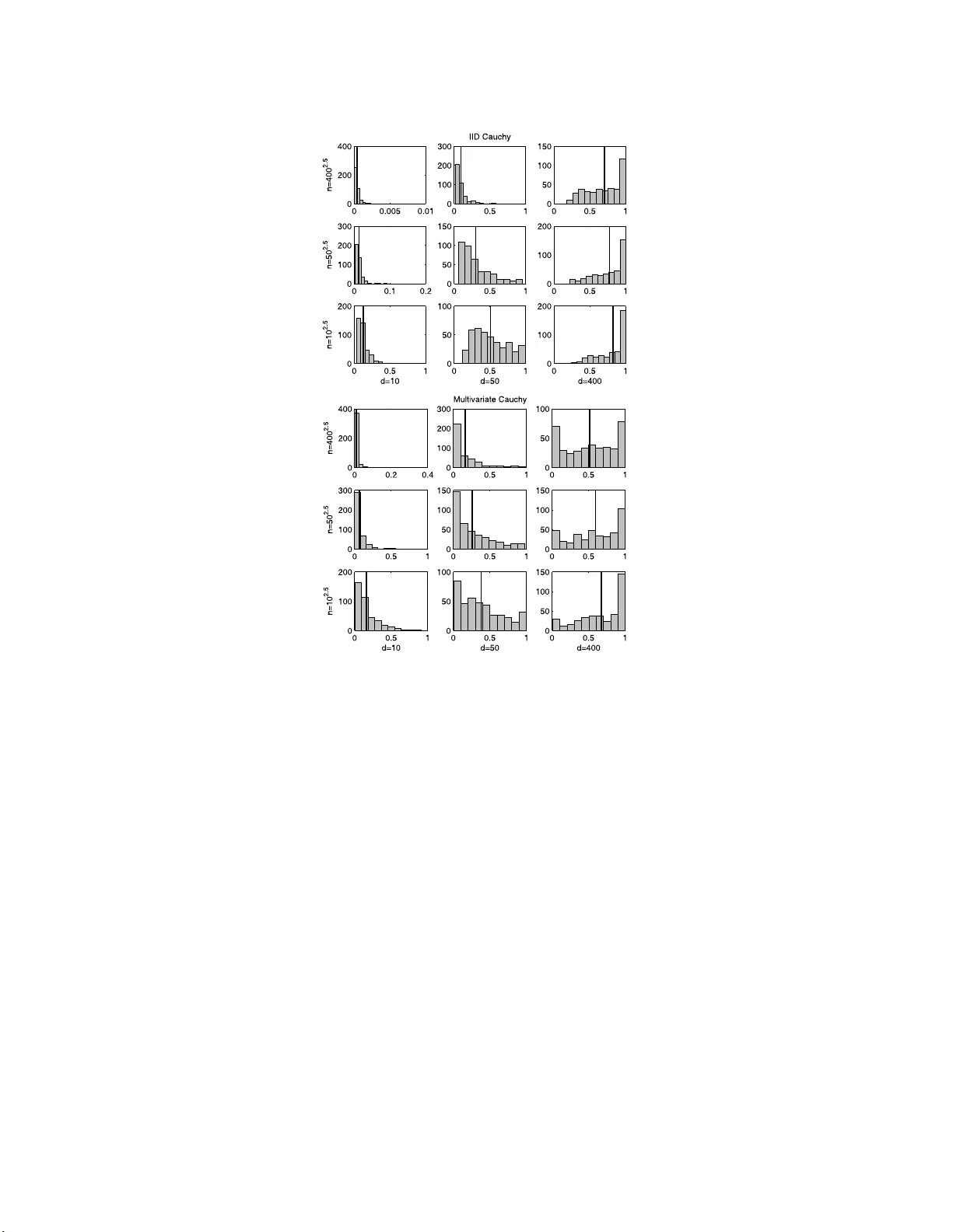
IMS Collectio ns Probability and Statistics: Essays in Honor of David A . F reedman V ol. 2 (2 008) 316–33 4 c  Institute of Mathematical Statistics , 2008 DOI: 10.1214/ 1939403 07000000 518 Curse-of-d imensionalit y revisited: Collapse of the particle filte r in v ery large scale systems Thomas Bengtsson 1 , P eter Bic k el 2 and Bo Li ∗ 3 Bel l L abs, University of California, Berkeley, and Tsinghua University Abstract: It has been widely realized that Monte Carlo methods (approxi- mation via a sample en sem ble) ma y fail in large sca le systems. This w ork offe rs some theoretical insight int o this phenomenon in the cont ext of the particle filter. W e demonstrate that the maximum of the weigh ts asso ciated wi th the sample ensemble conv erges to one as both the sample si ze and the system di- mension tends to infinity . Sp ecifically , under fairl y weak assumptions, if the ensem ble size gro ws sub-exponentially in the cub e ro ot of the system dimen- sion, the conv ergenc e holds for a single up date step in state-space models with independent and iden tically distri buted kernels. F urther, in an imp ortant sp e- cial case, m ore refined arguments show (and our simulations suggest) that the con v ergence to unit y o ccurs unless the ensemble grows super -exp onentially in the syste m dimension. The weigh t singularity is also established in models with more general multiv ariate likelihoo ds, e.g. Gaussian and Cauch y . Although pr e- sen ted in the con text of atmospheric data assi milation for numerical we ather prediction, our r esults are generally v alid for hi gh-dimensional particle filters. 1. In tro duction With ever increasing computing p ow er and data stora ge capabilities, very larg e scale scientific analyse s a re feasible a nd necessary (e.g. [ 8 ]). One impor tant appli- cation area of high-dimensional data a na lysis is the atmospheric sciences, where solutions to the genera l (in verse) problem of combining data and mo del quanti- ties a re co mmo nly required. F or instance, to produce real-time weather forecasts (including hurricane and severe weather warnings), satellite radia nce o bs e rv ations of h umidit y a nd radar backscatter of sea surface winds must b e co mbin ed with previous numerical foreca sts fro m atmo s pheric a nd o ceanic mo dels. T o suc h ends, recent work on n umerica l w ea ther prediction is cast in probabilistic or Ba y esian terms [ 10 , 21 , 26 ], and muc h fo cus in the literature o n the a ssimilation of da ta and n umerical mo dels p erta ins to the sampling o f high-dimensiona l proba bilit y densit y functions (pdf ) [ 1 , 1 8 , 25 , 27 ]. Motiv ated b y these sampling techniques, we inv es- tigate the dangers of naively using Mont e Carlo approximations to e s timate lar ge ∗ Supported in part b y National Natural Science F oundation of China (70621061 ). 1 Bell Labs, 600 Mountain Av en ue, Murray Hill, NJ 07974, USA, e-mail: tocke@re search. bell-labs.com 2 Unive rsity of Calif or nia, Departmen t of Sta tistics, 367 Ev ans Hall #3860, Berkeley , CA 9472 0- 3860, USA, e-mail: bickel@s tat.ber keley.ed u 3 Tsingh ua Univ ers it y , 440 W eilun Hall, School of Economics and Managemen t, Beijing 100084, China, e-m ai l: libo@sem .tsingh ua.edu.cn AMS 2000 subje ct classific ations: 93E11, 62L12, 86A22, 60G50, 86A32, 86A10. Keywor ds and phr ases: ensem ble forecast, inv erse pr oblem, M on te Carlo, multiv ar iate Cauc hy, multiv ariate l ikelihood, nume rical w eather prediction, sample ensemble, state-space model. 316 Curse-of-dimensionality r evisit e d 317 scale sys tems. Specifically , in the context of the pa rticle filter, we sho w that accurate estimation of (truly) high-dimensional p dfs req uir e ense mble s izes that essentially grow exp onentially with the sy s tem dimension. Some recent work in numerical weather pr ediction has extended K alman filter solutions to work efficiently in Gaussian systems with degr e e s of freedom exceeding 10 6 . O ne po pular extensio n is g iven by the ensembl e Kalman filter, a Mont e C a rlo based filter version whic h draws sa mples from the p osterior distribution of the at- mospheric state given the data and the mo del [ 6 , 11 ]. Ho wev er, the task of sampling in real-time fr o m such high-dimensiona l sys tems is conceptually non-trivial: com- putational re s ources limit s ample sizes to several orders of magnitude smaller than the system dimensio n. T o address sampling err ors asso ciated with small ensembles, v a rious approa ches leverage spars ity constra int s to attenuate spurious cor relations [ 15 , 1 7 , 25 ]. Moreov er, in the Gaussian case , for systems with a finite n umber o f dominant mo des, mo derate s ample sizes are sufficient to a c curately estimate p os- terior means and cov ar iances [ 1 2 ]. F or lo nger forecast lead times, the involv ed dynamical models exhibit strongly non-linear b ehavior and pro duce distinctly non-Gaussian forecast distributions (e.g. Figure 2, [ 3 ]). In these situations, optimal filtering req uires the use o f more fully Bay esia n filtering metho ds to combine data a nd mo dels. In the context o f o ceano- graphic data assimilation, one such approach is consider ed b y [ 27 ], who prop os es a sequential imp ortance s a mpling algorithm to obtain p osterior estimates of o ceanic flow structures. This method falls within the set of pr o cedures t ypically referred to as particle filters (e.g. [ 9 ]). Ba sed o n a finite set of sample po ints with a sso ciated sample-weigh ts, the par ticle filter seeks to propa gate the pr obability distribution of the unkno wn state fo rward in time using the system dynamics. Once new da ta is av ailable, Bay es theorem is used to re-nor malize the weights based on how “close” the asso ciated sa mple p oints ar e to the data. Although successfully a pplied to a v ariety of settings, particle filters often yield highly v a rying imp ortance weigh ts and are known to b e unstable even in low- order mo dels. Remedies to s tabilize the filter include r e-sampling (re- normalizing) the in volved empirica l mea sure at reg ular time interv als [ 14 , 1 9 ], marginalizing or r estricting the s ample space [ 20 , 22 ], and diversifying the sample (e.g. [ 13 ]). How ever, these a pproaches s e rve to improve filter p erforma nce in low-dimensional systems, but do not fundamentally addr e s s slow con vergence ra tes when the par ticle filter is applied in la rge s cale systems. In pa rticular, a s noted by e.g. [ 27 ] and [ 1 ], when applied to geo ph ysical mo dels of hig h dimension, sequential imp ortance sampling collapses to a p oint mass a fter a few (o r ev en one!) observ a tio n cycles. T o s hed light o n the effects of dimensionality on filter stabilit y , our work provides necessary sa mple size requirements to av oid w eight degener acies in truly larg e scale problems. This work is outlined as follows. The next section form ulates the problem of using ensemble metho ds for approximation purp oses in large scale sy stems, and provides motiv a ting simulations illustrating the p otential difficulties of high-dimensional es- timation. O ur main dev elopmen ts are then presented in Section 3 where w e giv e general conditions under which the maximum o f the sa mple weigh ts in the (likeli- ho o d ba sed) par ticle filter con verges to one if the ensem ble size is sub-exp onential in the cub e ro ot of the system dimension. The conv erg ence is established in a Gaus s ian context, but is also argued for observ ation mo dels with indep endent and identically distributed ( iid ) kernels. The v alidity of the weight co llapse in the case when the ensemble grows sub-exp onentially in the sys tem dimensio n (as sugg ested b y the simu lations) is discussed as an extension to the multiv ariate Ca uch y kernel and 318 T. Bengtsson, P. Bickel and B. Li its apparent slow er collapse. In Section 4, for completeness, in a Ga ussian context, we show that the particle filter b e haves as desired if the ensem ble size is sup er- exp o nent ial in the system dimension. A brief discussion in Section 5 concludes our work. 2. Model setting and motiv ation This se c tio n gives the model setting and describ es the Monte Carlo estimation prob- lem under considera tion. T o illustrate the difficulty of high-dimensional estimation, we also provide motiv ating e x amples that describ e the weigh t singular ity . 2.1. Mo del setting The statistical context in which we motiv a te our work is a s follows. Cons ider a set of n s ample p oints X = { X 1 , . . . , X n } , where X i ∈ ℜ d and b oth the sample size n and sy s tem dimension d a re “lar ge”. W e assume that the sample X is drawn randomly from the prior (or proposa l) distribution p ( X ). New data Y is related to the state X by the conditional density p ( Y | X ). F or concreteness , a functional relationship Y = f ( X ) + ε is ass umed, and ε is taken to b e indep endent the sta te X . The goa l is to estimate p osterior exp ectatio ns using the imp or tance r atio: i.e. , for some function h ( · ), we want to estimate E ( h ( X ) | Y ) = Z h ( X ) p ( Y | X ) p ( X ) R p ( Y | X ) p ( X ) dX dX, and use ˆ E ( h ( X ) | Y ) = n X i =1 h ( X i ) p ( Y | X i ) P n j =1 p ( Y | X j ) as an estimator. Based on this formulation, the w eights a ttached to each ensem ble mem ber (1) w i = p ( Y | X i ) P n j =1 p ( Y | X j ) are the primary ob jects of our study . As ment ioned, in large scale analyses, the weigh ts in ( 1 ) are highly v a riable a nd often pro duce estimates ˆ E ( · ) which are col- lapsed ont o a p oint mass with max ( w i ) ≈ 1 . F o r high-dimensional systems, this degeneracy is p erv asive and a pp ea r s to ho ld for a wide v ariety of prior and likeli- ho o d distributions. Next we illustrate the degeneracy o f the sa mple weigh ts as the dimensio n of X and Y gr ows large. 2.2. Motivating examples T o illustr ate the weigh t collapse of the par ticle filter w e simulate w e ig ht s from ( 1 ) for bo th a Gaussian a nd a Cauch y distributional setting. These densities were chosen to parallel the work of [ 27 ], whic h attempts to addr e ss par ticle filter co llapse by mo deling the obser v ation nois e using a heavy-tailed distribution. In our s imulations, the d × 1 obs e rv ation vector Y is r elated to the uno bs erved state v ariable X through the mo del Y = H X + ε . Here, the o bs erv ation op erator Curse-of-dimensionality r evisit e d 319 H is se t equal to the d × d iden tit y matrix, denoted I d , and the propo sal (i.e. forecast) distribution is ta ken as zero-mean Gaussian with cov ar iance cov ( X ) = I d , denoted X ∼ N (0 , I d ). These c ho ices for H and cov ( X ) allow us to stra ightf orwardly manipulate the system dimension, and to study the be havior of the maximum weigh t for v a rious choices of d and n . F or the Gaussia n case we let ε ∼ N (0 , I d ), while for the Cauch y c a se we in vestigate tw o scenarios. First, the c o mpo nent s of ε = [ ǫ 1 , . . . , ǫ d ] T are taken as iid Cauch y , where each co mpo nent ha s lo cation and scale parameters set equal to zer o and one, respec tively . Second, ε is tak en as m ultiv ar iate Cauch y , ag ain with lo ca tion and scale parameters equal to zero and one. In each sim ulation run o f the maximum weight , an obs e r v ation Y is drawn fro m p ( Y ) and a random sample o f n par ticles X 1 , . . . , X n , is obtained from p ( X ) = N (0 , I d ) . Then, given Y , the sample par ticles are re-weigh ted according to ( 1 ) and the maximum w eight, denoted w ( n ) , is determined. T o ev aluate the dep endence of w ( n ) on d and n , we v ary the s ystem dimension at three levels, and let the Monte Carlo sample s iz e increase p oly no mially in d at a rate o f 2.5, i.e. we s et n = d 2 . 5 . F o r the Gaussian setting, we let d = 1 0 , 50 , 10 0 and obtain n = 31 6 , 1767 6 , 100 000, while, for the Cauc h y settings, wher e co nv erge nce to unit y was observed to b e slow er, the maximum dimension is increased to d = 400 . Thus, for the Cauch y simu lations, we set d = 10 , 5 0 , 400 , a nd get n = 31 6 , 1767 6 , 320 0000. Our setup results in nine simulation sets each for the three distributional settings, and each set is based on 4 0 0 indep endent dr aws of w ( n ) . Histograms of the maximum w eight w ( n ) for the Gauss ian setting a r e display ed in Figure 1 . The effect of changing the dimension is represented column-wise, and the effect of changing the Mo nt e Carlo sa mple size is given row-wise. E a ch plo t also depicts the co rresp onding sample mean maximum w eig ht ˆ E ( w ( n ) ) as a vertical line. Fig 1 . Sampling distrib ut i on of w ( n ) for the Gaussian ca se. The nine plots show histo gr ams of w ( n ) with system dimension v aried c olumn-wise ( d = 10 , 50 , 100 ) and sampl e size varie d r ow-wise ( n = 10 2 . 5 , 50 2 . 5 , 100 2 . 5 ). The vert ic al line in e ach plot depicts ˆ E ( w ( n ) ) . Each histo gr am is ba se d on 400 simulations. 320 T. Bengtsson, P. Bickel and B. Li Fig 2 . Sampling distribution of w ( n ) for ε iid Cauchy (top p anel), and ε multivariate Cauchy (b ottom p anel). In ea ch p anel, the system dimension d is v arie d c olumn-wise ( d = 10 , 50 , 400 ), and the sample size is varie d r ow-wise ( n = 10 2 . 5 , 50 2 . 5 , 400 2 . 5 ). The vertic al line in e ach plot depicts ˆ E ( w ( n ) ) . Each histo gr am is ba se d on 400 simulations. As indicated, for a fixed sa mple size (i.e. within a r ow), the distribution of w ( n ) is dramatically shifted to the r ight, a nd we see that w ( n ) approaches unity as d grows. Moreov er, the same singularity is evident along the dia gonal from the lo wer left ( d = 10 , n = 316 ) to the upp er rig ht ( d = 100 , n = 1000 00) histogram. Hence, even as n gr ows at a p oly no mial rate in d , w ( n ) still approa ches unit y . The histograms in the t w o panels of Figure 2 show the simulation results for the Cauch y se ttings. As in the previous figure, the effect o f changing the dimension is given co lumn-wise , a nd the e ffect of v arying the ensemble size is given row-wise. Also depicted is the sample mea n maximu m w eight ˆ E ( w ( n ) ) as a v ertical line. F or the iid Cauch y case, display ed in the to p panel, for fixed n , the sampling distribution of w ( n ) is clearly shifted to the r ight as d increases. Moreover, similarly to the Gaussian results, the weight s ing ularity is ag ain evident in the histograms alo ng the diago na l where the s ample size grows as n = d 2 . 5 . As with the ii d setting, the histog rams of w ( n ) for the multiv aria te Cauch y cas e (b ottom panel) also demonstrate w eight collapse. How ever, as ca n b e seen, the co nv erg e nce is slow er. The r easons for the apparent slow er co lla pse will b e discussed in Section 3.3 . Curse-of-dimensionality r evisit e d 321 T o shed light o n the illustra ted weight colla pse, w e nex t present a formal study of the be havior o f the maximum imp ortance w eight. Sp ecifically , the next section develops conditions under which the maximum weigh t w ( n ) conv erg es to unit y . 3. T he singularity of the maximum weigh t for mo dels with iid kernels In this s ection, we mak e pr ecise the reaso ns for the previously descr ib ed weight collapse. The primary fo cus is on situations where the likeliho o d p ( Y | X ) is based on iid c o mpo nent s (or iid blo cks) and the pr op osal distr ibution p ( X ) is Gaussian. Our basic too l, given below in Lemma 3.1 , gives reasonable conditions under which the maximum weigh t based on the general form in ( 1 ) conv erges to unity as d and n grow to infinity . Our ma in insig ht is that, for larg e d , p ( Y | X i ) is o ften well approximated by the form (2) p ( Y | X i ) ∼ exp {− ( µd + σ √ dZ i ) } (1 + o p (1)) , where Z i follows the standar d normal distribution and where µ a nd σ a r e po sitive constants. The justification of this form is highlighted by the developmen ts in Sec- tions 3 .1 – 3.3 , and the conditions under whic h ( 2 ) produces weigh t c o llapse a re made precise b elow in Lemma 3 .1 . Note tha t, with Z ( i ) representing the i :th order statistic from an ensemble o f s ize n , the maximum weight w ( n ) behaves as w ( n ) ∼ 1 1 + P n ℓ =2 e − σ √ d ( Z ( ℓ ) − Z (1) ) . Thu s, to establish weigh t collapse, it suffices to show that the denominator in the ab ov e expre s sion co nv erges to unit y for large d . The following lemma g ives the strong version o f ( 2 ), which is needed for our conclusion, and formalizes the con- vergence. Lemma 3. 1 . L et S i , i = 1 , . . . , n, b e indep endent ra ndom variables with cumulative distribution function (c df ) G d ( · ) satisfying G d ( s ) = (1 + o (1))Φ( s ) over a suitable interval, wher e Φ( · ) is the c df of a st andar d normal distribution. Sp e cific al ly, we assume t her e exist t wo se quenc es α l n,d and α u n,d , wher e b oth α l n,d and α u n,d tend t o 0 as n and d go to infinity, such that, for s ∈ [ − d η , d η ] with 0 < η < 1 / 6 , we have (3) (1 + α l n,d )Φ( s ) ≤ G d ( s ) ≤ (1 + α u n,d )Φ( s ) . L et S (1) ≤ · · · ≤ S ( n ) b e the or der e d s e quenc e of S n , . . . , S n , and define, for some σ > 0 , T n,d = P n ℓ =2 e − σ √ d ( S ( ℓ ) − S (1) ) . Then, if log n d 2 η → 0 , E ( T n,d | S (1) ) = o p (1) . A pro of of the lemma is provided in the Appendix. An immediate implication o f this result is weight co llapse, i.e. if log n d 2 η → 0, we hav e w ( n ) P − → 1 . With the normality condition ( 3 ) v alid for η < 1 2 , o ur conclusion would hold, effectiv ely , whenever log n d → 0; rather than, as shown a b ov e, for log n d 1 / 3 → 0. Unfor- tunately , unless G d ( s ) ≡ Φ( s ), o ur pro o f is v alid only for η < 1 6 . How ever, using 322 T. Bengtsson, P. Bickel and B. Li more refined ar guments in conjunction with Lemma 2 .5 of [ 23 ] one ca n s how that, under the co nditions of Lemma A.1 (see Appendix), o nly log n d 1 / 2 → 0 is requir e d for collapse. F urthermore, using sp ecia lize d a rguments, we can show that in the Gaussian prior -Gaussian lik eliho o d setting, log n d → 0 is the necessar y condition for collapse. W e do not descr ib e these ar g ument s in detail, but focus instea d o n Lemma 3.1 which can b e a pplied mo re broadly . W e next turn our attention to high-dimensio nal, linear Gaussian s ystems. 3.1. Gaussian c ase W e assume a data mo del given b y Y = H X + ε, where Y is a d × 1 vector, H is a known d × q matrix, a nd X is a q × 1 vector. Both the prop osal distr ibution and the err or distribution are Ga ussian with p ( X ) = N ( µ X , Σ X ) and p ( ε ) = N (0 , Σ ε ), and the no ise ε is ta ken indep endent of the state X . Since the data mo del ca n b e pre-rotated by Σ − 1 / 2 ε , we set Σ ε = I d without loss of generality (wlog). Mo reov e r , since E Y = E H X , w e can replace X i b y ( X i − E X i ) and Y by ( Y − E Y ) and leav e p ( Y | X ) unchanged. Hence, wlog we a ls o set µ X = 0. Mo reov er , define, for conformable A a nd B , the inner pro duct h A, B i = A T B (where the super s cript T denotes matrix transp o se), and let k A k 2 = h A, A i . With p ( Y | X ) ∼ N ( H X , I d ), the weigh ts in ( 1 ) can b e expres sed as (4) w i = exp  − k Y − H X i k 2 / 2  P n j =1 exp  − k Y − H X j k 2  2) . T o establish w eig ht collapse for high-dimensional Gaussian p ( Y | X ) and p ( X ), we show that, under reas o nable assumptions, the ex p o nen t in ( 4 ) satisfies the con- ditions of Lemma 3.1 . Let d ′ = rank ( H ). With λ 2 1 , . . . , λ 2 d ′ the singular v alues o f cov ( H X ), define the d ′ × d ′ matrix D = diag ( λ 1 , . . . , λ d ′ ). Then, with Q an orthogona l matrix obtained b y the sp ectral decomp os itio n of cov ( H X ), define the d ′ × 1 vector V such that Q T H X = D V . Note that V i corresp onding to X i is N (0 , I d ′ ). Since Q is or thogonal, we can write (5) k Y − H X i k 2 = k Q T Y − D V i k 2 = d ′ X j =1 λ 2 j W 2 ij + d X j = d ′ +1 ǫ 2 0 j , where, conditional on Y , [ W i 1 , . . . , W id ′ ] T is N ( ξ , I d ′ ), and where ǫ 0 j is the j :th comp onent o f the o bs e r v ation noise vector ε . The mean vector ξ = [ µ 1 , . . . , µ d ′ ] T is given by (6) ξ = D − 1 Q T Y = V + D − 1 ε ′ , where V a nd ε ′ are indep endent N (0 , I d ′ ) . Now, for i = 1 , . . . , n , define (7) S i = P d ′ j =1 λ 2 j ( W 2 ij − (1 + µ 2 j ))  2 P d ′ j =1 λ 4 j (1 + 2 µ 2 j )  1 / 2 . Note that the second term in ( 5 ) is constant fo r every X i , and will not influence the weigh t w i . W e assume, Curse-of-dimensionality r evisit e d 323 A1. There is a p ositive consta n t δ such that δ < λ 1 , · · · , λ d ′ ≤ 1 δ ; and A2. σ 2 d ′ = 2 d ′ P d ′ j =1 λ 4 j (1 + 2 µ 2 j ) → σ 2 > 0. With these assumptions, L emma A.2 of the App endix es tablishes that the uni- form no rmality co ndition given b y ( 3 ) holds for the standardized terms defined in ( 7 ). The res ult is v alid for any 0 < η < 1 / 6 a nd is based on Theor em 2.5 o f [ 23 ]. Note that, from ( 6 ) and ( 7 ), we ca n write k Y − H X i k 2 ∝ σ √ d ′ S i (1 + o (1)) + d ′ X j =1 λ 2 j (1 + µ 2 j ) , where o (1) is indep endent of the subscript i . W e can now state the following pr op osition. Prop ositio n 3. 2. Under assumptions A1 and A2 , if log n d ′ 2 η → 0 with 0 < η < 1 / 6 , we have w ( n ) P → 1 . Prop osition 3.2 follows by Lemma A.2 (App endix) and Lemma 3.1 . The a bove result implies that, unless n grows super -exp onentially in d ′ 1 / 3 , we hav e weigh t collapse. How ever, a s we show in Section 4 , the weigh t singularity is av oided when d ′ is b ounded, or, more g enerally , when log n/d ′ → ∞ . T o establish the exact bo undary o f co llapse in the Gaussia n setting, a closer analysis of the chi-squared distribution ( c.f. k Y − H X i k 2 ) with d ′ degrees of freedom is needed. In particular, using the Poisson s um formula for the tails of the gamma distribution, it can b e ar gued that colla pse o ccurs if log n/d ′ → 0 . Essentially , with G d ( s ) = Φ( s ) and for suitable σ 2 , we can show E ( T n,d | S (1) ) ∼ r 2 log n σ 2 d ′ , in probability . As ment ioned, we do not describ e the sp ecifics o f this argument, but fo c us instead on the mo r e gener al result of Lemma 3.1 . Next we turn our attention to settings w her e b oth the observ ation and state vectors consist of iid co mpo nen ts. 3.2. Gener al ii d kernels It may be sp eculated that the weight singularity can be amelio r ated b y the use of a heavy-tailed kernel. How ever, w e a rgue that, as long as the comp onents of the observ atio n noise are iid and H is the identit y matrix, we still exp ect weigh t collapse for larg e d . The mo del setting is Y = X + ε . L e t X ik be the k :th comp onent of X i . W e take X ik iid with common densit y g ( · ), and take the comp onents of ε = [ ǫ 1 , . . . , ǫ d ] T iid with common density f ( · ) . Then, with ψ ( · ) = lo g f ( · ), given Y = [ y 1 , . . . , y d ] T , we can write the weigh ts fro m ( 1 ) as w i = exp  P d j =1 ψ ( y j − X ij )  P n k =1 exp  P d j =1 ψ ( y j − X kj )  . Define V ij = ψ ( y j − X ij ) , and let µ ( y j ) = E ( V ij | y j ) and σ 2 ( y j ) = E ( V 2 ij | y j ) − µ 2 ( y j ) , wher e the e x pec ta tions are ev aluated under f ( · ). With these quantit ies, let S i = P d j =1 ( V ij − µ ( y j ))  P d j =1 σ 2 ( y j )  1 / 2 , 324 T. Bengtsson, P. Bickel and B. Li for i = 1 , . . . , n . Aga in, let S (1) ≤ · · · ≤ S ( n ) be the order ed sequence of S 1 , S 2 , . . . , S n . Now, in ana lo gy to P rop osition 3.2 : if log n d 2 η → 0 , a nd (i) the sequence { V ij − µ ( y j ) } d j =1 satisfies the co nditions of Theorem 2.5 of [ 23 ]; and (ii) 1 d P d j =1 σ 2 ( y j ) P → σ 2 > 0, then the maximum weight w ( n ) conv erg es in proba bilit y to 1 . T o v er ify the nor mality approximation in ( 2 ) for S i , it is ea s y to chec k that σ 2 = E σ 2 ( y 1 ) < ∞ , and max j   ψ ( y j − X ij )   = o p ( d 1 / 2 ) uniformly in i . The nex t prop osition gives chec k able, alb eit s tr ong c o nditions, leading to weigh t collaps e . Prop ositio n 3. 3. L et the c omp onents of X 0 = [ X 01 , . . . , X 0 d ] T b e iid with density g ( · ) , and let t he c omp onent s of ε = [ ε 1 , . . . , ε d ] T b e iid with density f ( · ) . Set Y = X 0 + ε . L et X 1 , . . . , X n b e iid ve ctors, e ach with iid c omp onent s X ik with c ommon density g ( · ) . Assu me that f , g ar e s u ch that E [ f t ( Y j − X 1 j )] < ∞ , for | t | < δ with δ > 0 . Then, wi th T n,d = P n ℓ =2 e − σ √ d ( S ( ℓ ) − S (1) ) , if log n d 2 η → 0 fo r 0 < η < 1 / 6 , we have, E ( T n,d | S (1) ) P → 0 . The result fo llows from Lemma 3.1 and Lemma A.1 . Note that mos t common f , g , e.g. the Ga ussian a nd Cauch y , satisfy the conditions of Pr opo sition 3.3 . If H is not the identit y , our conclusion may still hold for log n d 1 / 3 → 0. F or general H , set U i = H X i and le t U ik be the k -th component o f U i . With this quantit y , provided the regular it y conditions ar e sa tisfied, we may apply Theorem 3.23 of [ 23 ] to the terms S ψ, i = P d j =1 ψ ( y j − U ij ) − µ ( y j ) σ √ d , where µ ( y j ) and σ are suitable constants. Next we turn o ur attention to the cas e when the obser v ation noise v ector follows the mult iv a r iate Cauch y distribution. 3.3. Multivari ate Cauchy c ase Our development s so far ha v e considered se ttings where p ( Y | X ) is o f multi plica- tiv e form; in particular, mo del s e ttings with iid likelihoo d kernels (o r iid blo cks of o bs e r v ations). W e now discuss extensions o f our results to include multiv a riate likelih o o d functions. Ex c e pt for the multiv ariate Gauss ian case, how ev er, whic h can be addressed by rotation (see Section 3.1 ), w e note that no genera l result exists that addresses a wide rang e of multiv ariate likelih o o d functions. Here, we fo cus on the mu ltiv ar iate Cauch y distribution, which, in the co nt ext of o ce a nogra phic data assimilation, was pro po sed by [ 27 ] to avoid weight collapse. W e still entertain the da ta mo del Y = H X + ε and, as in the previous sec tio n, restrict H = I d . Her e, w e let p ( X ) = N (0 , I d ) and take the nois e vector ε to follow the multiv ariate Cauch y distribution. W e note that the m ultiv aria te Cauch y distri- bution is equiv alent to the m ultiv ar iate t-distribution with 1df (e.g. [ 2 ], pa ge 55). Then, given data Y and a sample X i ∼ N (0 , I d ) , i = 1 , . . . , n, the multiv ariate Cauch y weigh ts are given by w i = (1 + k Y − X i k 2 ) − d +1 2 P n j =1 (1 + k Y − X j k 2 ) − d +1 2 . Curse-of-dimensionality r evisit e d 325 Now, with k Y − X [1] k ≤ . . . ≤ k Y − X [ n ] k the order statistics, we expres s the w e ig ht s in familiar form, i.e. w ( n ) =   1 + n X j =2 exp  − d + 1 2  log(1 + k Y − X [ j ] k 2 ) − log (1 + k Y − X [1] k 2 )     − 1 . T o arg ue w ( n ) ≈ 1 for la rge d , we note first that the scenar io c onsidered here is closely related to the Gaussia n pr ior-Gaussia n likelihoo d case. Prop ositio n 3.4. L et X b e zer o-me an Gaussian with cov ( X ) = I d and take ε to fol low the m ultivariate Cauchy distribution. Then, with Y = X + ε , as d → ∞ , we get p ( X | Y ) L − → N  Y d k Y k 2 , (1 − d k Y k 2 ) I d  . The co nv ergence in Pro po sition 3.4 is in the sense that the finite dimensional distributions on b oth sides conv er ge to the same limit. Thus, we r each the s omewhat surprising co nclusion that the p osterior distribution of X g iven Y is Gauss ian, but with parameters dep ending on the data. The result is prov ed in the App endix. In the App endix we also detail the heuris tic arg umen t that, as in the Gaussian- Gaussian case, the non-central χ 2 d ( σ 2 d ) distribution b ehaves sufficiently like N (( σ 2 + 1) d, 2(1 + 2 σ 2 ) d ) to per mit exact r eplacement in our developments. W e then r ea ch the conclusion of s low er weight co llapse for large n and d , as substa ntiated by our simulations. Sp ecifically , we a rgue that the average rate needed for co lla pse is q log n d   log  q log n d    → 0. F o r the Gauss ia n setting, the next section shows that weigh t collapse can b e av oided for sufficiently lar ge ensembles 4. Consistency of Gaussian particle filter As a complement to the developmen ts in the previo us section, we provide a con- sistency a rgument for the type of estimators of E ( h ( X ) | Y ) that are under consid- eration here. The dev elopments a re made in a Gauss ian context and we consider settings wher e b oth d and n a re larg e. Sp ecifically , if lo g n/d → ∞ , w e show co n- sistency of P n i =1 w i h ( X i ) as an estimator of E ( h ( X ) | Y ) . Suppos e we have a random s a mple { X 0 , X 1 , . . . , X n } , where X i ∼ N (0 , I d ) . As in the sim ulation s ection, let the data Y 0 be collected through the mo del Y 0 = X 0 + ε , where ε ∼ N (0 , I d ) is independent of X i . With p ( Y | X ) = N (0 , I d ), let { w 1 , . . . , w n } be the weigh ts obtained by ( 1 ). Now, choo se X ∗ i from { X 1 , . . . , X n } with proba bilities pr op ortional to { w 1 , . . . , w n } . Then, with δ ( · ) repres ent ing the delta function and ˜ p ( X | Y 0 ) = P n j =1 w i δ ( X i ), we hav e X ∗ i ∼ ˜ p ( X | Y 0 ). F urther, the exp ectation of h ( X ∗ ) (under the empirical measure) is given b y E ∗ ( h ( X ∗ ) | Y 0 ) = P n j =1 w i h ( X i ) . With this setup, the follo wing result establishes cons is tency of P n i =1 w i h ( X i ) as an estimator of E ( h ( X ) | Y ) . Prop ositio n 4. 1. L et h ( · ) b e a b ounde d function fr om ℜ d to ℜ . D efine E ∗ h ( X ∗ ) ≡ P n j =1 w i h ( X i ) , the exp e ctation under the (pr eviously define d) empiric al me asur e ˜ p ( X | Y 0 ) , and let E 1 ( · ) denote exp e ctation evaluate d under the (tru e) p osterior p ( X | Y 0 ) . Then, if log n/ d → ∞ , | E ∗ h ( X ∗ ) − E 1 h ( X ) | P − → 0 . 326 T. Bengtsson, P. Bickel and B. Li The result is prov ed in the Appendix. W e note that Pro po sition 4.1 is v alid for fi- nite dimensional measures. The next coro llary follows as an immediate consequence of the established conv ergence. Corollary 4. 2. L et { X ∗ 1 , . . . , X ∗ n } b e a r andom sample fr om p ∗ ( X | Y 0 ) . F u rther, with k fix e d, let ν ( x ∗ 1 , . . . , x ∗ k ) b e any r andom variable dep ending on the first k c o or dinates of X ∗ i . Then, with δ ν ( · ) r epr esenting the delta function for ν ( · ) , as log n/d → ∞ , 1 n n X j =1 δ ν ( x ∗ 1 , . . . , x ∗ k ) L − → N  1 2 [ y 01 , . . . , y 0 k ] T , 1 2 I k  . The results extend to include Y = H X + ε, wher e rank ( H ) = d ′ < ∞ . O f course, p ( Y | X ) and p ( Y ) hav e to b e changed in the developmen ts to acco mmo date arbitrary H , but we a gain have no collapse provided log n/d ′ → ∞ . 5. Discussion The collapse of the weigh ts to a p oint mass (with max ( w i ) ≈ 1) lea ds to disastrous behavior of the par ticle filter. One intuition ab out such weigh t-co llapses is well known, but here made precise in terms of d and n : Monte Ca rlo do es not work if we wish to compute d -dimensional integrals with r e s pec t to pro duct meas ures. The reason is that w e are in a situation where the prop osal distribution p ( X ) a nd the desired sampling distribution are approximately mutually singula r and (essentially) hav e disjo int suppo rt. As a consequence, the density of the desired distribution at all p oints of the prop osed ensem ble is small, but a v anis hing fraction o f densit y v a lues predominate in relation to the other s. Our dev elopmen ts demonstrate that br ute- fo r ce-only implemen tatio ns of the pa r- ticle filter to descr ibe high-dimensio nal p oster ior proba bilit y distributions will fail. Our work ma kes explicit the r ates at which sample sizes must grow (with resp ect to system dimension) to av oid singularities and degeneracies. In pa rticular, we give necessary b ounds o n n to av oid convergence to unity of the maximum imp ortance weigh t; and, natura lly , accurate estimation will r equire ev e n lar ger sample sizes than those implied by our r esults. Not surprising ly , weigh t degenera cies ha ve b een ob- served in geophysical s ystems of mo derate dimension ([ 1 , 3 ]; als o, C.Snyder/NCAR & T. Ha mill/NOAA , per s onal communication, 2 0 01). The usual manifestation o f this degener acy a re Monte Ca rlo samples that are to o “clos e ” to the data, quickly pro ducing singular proba bilit y measures, in particular as the filter is cycled over time. The o bvious remedy to this phenomenon is to a chiev e so me form o f dimension- ality reduction, a nd the high-dimensio nal for m in which the data are presented is t ypically op en to such reduction with subse quent effective ana ly sis. F o r instance, in the cas e of the ens e m ble Ka lman filter, by imp osing s parsity constraints through spatial lo calizatio n ([ 15 , 17 ]; see a ls o, [ 12 ]). Be that as it may , as shown in this work, for fully Bayesian filter analys es of high-dimensional sys tems, such reduc- tion beco mes essential lest spurious sample v a riability is to dominate the po sterior distribution. In the co nt ext of numerical weather prediction, one a pproach to dimension re- duction may b e to condition sample draws on a larger information set. One idea is given by [ 4 ], who constructs prop osal distributions by incorp ora ting dynamic infor- mation in a low-order mo del. Other examples o f geophysically co nstrained sampling Curse-of-dimensionality r evisit e d 327 schemes ar e given by Bayesian Hierarchical Mo dels (e.g. [ 16 , 28 ]), but require com- putationally heavy , c ha in-based sampling and th us do not extend in an y obvious manner to re a l-time applications. A more via ble po ssibilit y for rea l-time applica- tions in a larg e scale system is to break the system into lo w er-dimensional sets, and then sequen tially p erfor m the sa mpling as in [ 3 ]. Another approach may be to condition the draws on low er- dimensional sufficient statistics ([ 5 , 24 ]). A nov el idea to improving conv er gence in the Baysian filter cont ext is considered by [ 29 ] in the co nt ext of image matching and retriev al. F o r the purp ose of v alidating the exclusion of pa rts o f the sample spa c e which app ear unint eresting given the data, and to sp eed up the a lg orithm, they use information theor y to restr ict the sa mple space by explicitly incorp o r ating (drawing) samples of low probability . App endix W e first introduce tw o lemmas that p ertain to uniform normal approximations of the distribution o f independent s ums. Such sums app ear in the formulation of the filter weigh ts throug hout our work. V a lid for mo derately larg e deviations, the fir st result (Lemma A.1 ) is a combination of Theorem 2.5 and Theorem 1.31 in [ 23 ] and is stated here without pro of. The next res ult (Lemma A.2 ) is given for the purp ose of verifying the Lyapuno v quotients conditions app earing in Lemma A.1 . Lemma A. 1. L et ξ 1 , . . . , ξ d b e indep endent r andom variables with E ξ j = 0 and σ 2 j = V ar ( ξ 2 j ) . S et S d = 1 B d ( ξ 1 + · · · + ξ d ) , wher e B 2 d = P d j =1 σ 2 j , and define the Lyapunov quotients L k,d = 1 B k d d X j =1 E   ξ j   k , k = 1 , 2 , . . . . If B d = σ d 1 / 2 (1 + o (1)) , τ d = cB d (some σ, c > 0 ), and L k,d ≤ k ! /τ k − 2 d , k = 3 , 4 , . . . , then t he c df of S d , denote d G d ( · ) , satisfies (some C > 0 )     G d ( x ) Φ( x ) − 1     ≤ C | x | 3 d 1 / 2 , − d η ≤ x ≤ 0 , η < 1 / 6; and the survival function, ¯ G d ( · ) = 1 − G d ( · ) , satisfies     ¯ G d ( x ) ¯ Φ( x ) − 1     ≤ C | x | 3 d 1 / 2 , 0 ≤ x ≤ d η , η < 1 / 6 . Thus, under the outline d c onditions, the uniform normal appr oximations G d ( s ) = (1 + o (1))Φ( s ) , and ¯ G d ( s ) = (1 + o (1)) ¯ Φ( s ) hold, r esp e ctively, over the int ervals [ − τ η d , 0] and [0 , τ η d ] for η < 1 / 3 . The lemma is the bas is for the norma lit y conditions o f Lemma 3.1 . W e note tha t the condition on L k,d is satisfied in the iid ca se if E e tξ j < ∞ , for | t | ≤ δ, δ > 0 . Lemma A.2. L et Z j , j = 1 , . . . , d, b e iid N(0,1). L et 0 < δ ≤ λ 1 ≤ · · · ≤ λ d ≤ 1 δ and µ 1 , . . . , µ d b e such that (8) 0 < m < σ 2 d = 2 d d X j =1 λ 4 j (1 + 2 µ 2 j ) ≤ M < ∞ , 328 T. Bengtsson, P. Bickel and B. Li for some c onstants m, M . Then, with σ 2 d as define d in ( 8 ), (9) σ − k/ 2 d d X j =1 λ 2 k j E   ( Z j + µ j ) 2 − (1 + µ 2 j )   k ≤ C k k ! d − ( k − 2) 2 , for al l k = 3 , 4 , . . . and a un iversal c onstant C = C ( δ, m, M ) . The remainder of the Appendix is devoted to the pro ofs of the presented lemmas and pr op ositions. The pro ofs a re given in the order in which the results a pp ea r in the text. Pr o of of L emma 3.1 Let S j ( j = 1 , . . . , n ) be a s defined in the lemma. Before pro ceeding, we note some impo r tant results/ facts. First, it is well known that (10) p 2 log n  S (1) + p 2 log n − log log n + log(4 π ) 2 √ 2 log n  L → U, where U has a Gumbel distribution (see, e.g ., [ 7 ], p. 47 5). Second, by assumption, √ 2 log n d η → 0 for 0 < η < 1 / 6 , whic h allows us to use the normal appr oximation defined in ( 3 ). Third, w e mak e frequent use of Mill’s ratio: i.e., ¯ Φ( x ) ∼ φ ( x ) x , as x → + ∞ . Now, note that (11) E ( T n,d | S (1) ) = ( n − 1) R ∞ S (1) exp  − σ √ d ( z − S (1) )  dG d ( z ) ¯ G d ( S (1) ) , since, given S (1) , the r emaining ( n − 1) observ a tions are iid w ith cumulativ e density function (cdf ) e q ual to G d ( z ) / ¯ G d ( S (1) ) , z ≥ S (1) . By ( 10 ) and ( 3 ) we see that the denominator of the right hand side co nv erges to 1 in pro ba bilit y . T o ev a lua te the n umerator of ( 11 ), w e break the in teg ral into tw o parts: the first part yields the in tegral from S (1) to d η , a nd the second pa r t yields the tail integral from d η to ∞ . W e now show that b oth in tegrals conv erg e to 0 in pro bability . F o r the first par t, using in teg ration by parts (t wice) along with the approximation in ( 3 ), we can write Z d η S (1) exp  − σ √ d ( z − S (1) )  dG d ( z ) = G d ( d η ) exp  − σ √ d ( d η − S (1) )  − G d ( S (1) ) + Z d η S (1) exp  − σ √ d ( z − S (1) )  G d ( z ) dz =  G d ( d η ) − Φ( d η )  exp  − σ √ d ( d η − S (1) )  −  G d ( S (1) ) − Φ( S (1) )  + (1 + o (1)) Z d η S (1) exp  − σ √ d ( z − S (1) )  φ ( z ) dz . Now, again by as s umption, (12) ( n − 1) G d ( d η ) exp  − σ √ d ( d η − S (1) )  ≤ ( n − 1) G d ( d η ) ∼ ( n − 1)Φ( d η ) = o (1) . Curse-of-dimensionality r evisit e d 329 Analogously , ( n − 1)Φ( d η ) exp  − σ √ d ( d η − S (1) )  = o p (1). Hence, we hav e derived that (13) ( n − 1)  G d ( d η ) − Φ( d η )  exp  − σ √ d ( d η − S (1) )  = o p (1) . F urther , by ( 10 ) and ( 3 ), (14) ( n − 1)  G d ( S (1) ) − Φ( S (1) )  = o (1)( n − 1) G d ( S (1) ) . Let S b e an iid c o py o f S 1 . Then G d ( S ) is uniformly distributed on [0,1 ], and (15) E  G d ( S (1) )  = E  P ( S ≤ S 1 , . . . , S ≤ S n | S )  = E  ([ ¯ G d ( S )] n  = 1 n + 1 . Combinin g ( 14 ) and ( 15 ) yields (16) ( n − 1 )  G d ( S (1) ) − Φ( S (1) )  = o p (1) . Moreov er, by assumption σ √ d + S (1) ∼ σ √ d − √ 2 log n → ∞ . Thus, we get, aga in in light of ( 10 ), ( n − 1 ) Z d η S (1) exp  − σ √ d ( z − S (1) )  φ ( z ) dz ≤ ( n − 1) exp  σ √ dS (1) + σ 2 d/ 2  ¯ Φ( S (1) + σ √ d ) + √ d ( n − 1 ) ¯ Φ( d η ) ∼ ( n − 1 ) exp  σ √ dS (1) + σ 2 d/ 2  φ ( S (1) + σ √ d ) S (1) + σ √ d + √ d ( n − 1 ) ¯ Φ( d η ) = ( n − 1 ) e xp  − S 2 (1) / 2  √ 2 π ( S (1) + σ √ d ) + √ d ( n − 1 ) ¯ Φ( d η ) = o p (1) , The implication of the last inequality , in conjunction with ( 13 ) and ( 16 ), yields ( n − 1 ) Z d η S (1) exp  − σ √ d ( z − S (1) )  dG d ( z ) = o p (1) . By assumption, the second part of the integral in ( 11 ) is b ounded by σ √ d ( n − 1 ) ¯ G d ( d η ) = σ √ d ( n − 1 ) ¯ Φ( d η ) ∼ σ √ d ( n − 1 ) φ ( d η ) d η = o (1) . W e hav e shown that the numerator of the right hand side of ( 11 ) co nv erges to 0 in probability . This completes the pro of. Remark. If the normal approximation is g o o d enough to av oid the left bo undary term in the integration b y parts, we b elieve the conv ergence rate to b e dominated b y the quantit y Z ∞ S (1) exp  − σ √ d ( z − S (1) )  d Φ( z ) . As can b e seen in the pro of, b y ( 10 ), Z ∞ S (1) exp  − σ √ d ( z − S (1) )  d Φ( z ) ∼ C ( n − 1 ) exp  − S 2 (1) / 2  √ 2 π ( S (1) + σ √ d ) = O p  r log n d  . 330 T. Bengtsson, P. Bickel and B. Li Pr o of of Pr op osition 3.4 . Let Z i iid ∼ N (0 , 1) , i = 0 , . . . , d , and define ε = [ Z 1 , . . . , Z d ] T / | Z 0 | . That is, ε follows the multiv aria te Cauch y distribution. Let the data be defined by Y = X + ε . Conditional on ( Y , Z 0 ), the p osterior distribution of X is Gaussian, i.e. p ( X | Y , Z 0 ) = N  | Z 0 | 2 1 + | Z 0 | 2 Y , 1 1 + | Z 0 | 2 I d  . W e approximate k Y k 2 = k X k 2 + 2 h X, ε i + k ε k 2 = d + O ( √ d ) + 2 O ( √ d ) + d + O ( √ d ) | Z 0 | 2 , = d (1 + O (1 / √ d ) + 1 + O (1 / √ d ) | Z 0 | 2 ) , W e hav e k Y k 2 = d (1 + 1 | Z 0 | 2 )(1 + o (1)), and (1 + 1 | Z 0 | 2 ) = k Y k 2 d (1 + o (1)). Substituting in p ( X | Y , Z 0 ), we obtain p ( X | Y ) L − → N  Y d k Y k 2 , (1 − d k Y k 2 ) I d  . Heuristic pr o of for m u ltivariate Cauchy c ase Assume log n d 1 / 3 → 0 and let k Y − X [1] k ≤ · · · ≤ k Y − X [ n ] k b e the order statistics. W e hav e w i ∝  1 + k Y − X i k 2  − d +1 2 , and can write, as usua l, w ( n ) = 1 1+ T n,d , where (17) T n,d = n X j =2 exp  − d + 1 2 [log(1 + k Y − X [ j ] k 2 ) − log (1 + k Y − X [1] k 2 )]  . The nois e vector follows the multiv ariate Cauch y dis tr ibution, i.e. ε = [ Z 1 ,...,Z d ] T | Z 0 | , where Z 0 , Z 1 , . . . , Z d are iid N (0 , 1). Note that 1 + k Y − X i k 2 = (1 + k Y k 2 + d )  1 + ( k X i k 2 − d ) − 2 h Y , X i i 1 + k Y k 2 + d  . Now, similarly to the developments in Prop os ition 3.4 , given Z 0 , 1 + k Y k 2 + d = d (2 + 1 Z 2 0 )(1 + O p ( d − 1 / 2 )) , b y the central limit theor em. Moreov e r , (18) log(1 + k Y − X i k 2 ) − log (1 + k Y − X [1] k 2 ) = log (1 + S i ) − log (1 + S (1) ) , where S i = P d j =1 [( X 2 ij − 1) − 2 Y j X ij ] 1 + k Y k 2 + d = P d j =1 [( X 2 ij − 1) − 2 Y j X ij ] d (2 + 1 Z 2 0 ) (1 + O p ( d − 1 / 2 )) . (19) Curse-of-dimensionality r evisit e d 331 Some calculations show that, conditioning on Z 0 , the a symptotic v a riance of S i is given by σ 2 ( Z 0 ) d , where σ 2 ( Z 0 ) = 6+ 4 Z 2 0 (2+ 1 Z 2 0 ) 2 . Now, up to a scale factor, the S i ’s are the same (conditionally indep endent ) summands as in the Gaussian-Gaussia n case. So, we can hop e fo r a uniform Gaussian approximation. W e proceed a s if it were exa ctly Gaussian with mean 0 and v ariance given by the asymptotic v alue σ 2 ( Z 0 ) d . W e now expa nd the logarithm in ( 19 ) using S i = O p ( d − 1 / 2 ). With W 1 , . . . , W n iid N (0 , 1) and with W (1) the minim um, we obtain exp  − d + 1 2 [log(1 + S i ) − log (1 + S (1) )]  = exp  d 1 / 2 2  [ σ ( Z 0 ) W i − σ 2 ( Z 0 ) 2 d 1 / 2 W 2 i ] − [ σ ( Z 0 ) W (1) − σ 2 ( Z 0 ) 2 d 1 / 2 W 2 (1) ]  (20) × (1 + o p (1)) . Since | W (1) | = O p ( √ log n ) , we heuristically neglect the cubic term in the expression which is O p ( | W 3 (1) | /d 1 / 2 ) = o p ( W 2 (1) ) . W e now pro ceed as in the Ga ussian-Gaussia n ca se neglecting the o p (1) term. W e hav e, (21) E ( T n,d | W (1) , Z 0 ) ≈ ( n − 1) q − 1 d ( W (1) ) R ∞ W (1) q d ( w ) φ ( w ) dw ¯ Φ( W (1) ) , where q d ( w ) = exp  − d 1 / 2 2 σ ( Z 0 ) w + σ 2 ( Z 0 ) 4 w 2  . Letting A = σ 2 ( Z 0 ) 2 , B = σ ( Z 0 ) 2 , using the approximation ¯ Φ( W (1) ) ≈ 1 for the denominator alo ng with Mill’s r atio, we compute the integral in ( 21 ) to get E ( T n,d | W (1) , Z 0 ) ≈ n − 1 q d ( W (1) )(1 − A ) 1 / 2 ¯ Φ  (1 − A ) 1 / 2 W (1) (22) + d 1 / 2 B (1 − A ) − 1 / 2  exp  dB 2 2(1 − A )  ≈ n − 1 √ 2 π (1 − A ) 1 / 2 exp  − W 2 (1) 2  (23) ×  (1 − A ) 1 / 2 W (1) + d 1 / 2 B (1 − A ) − 1 / 2  − 1 ≈ √ 2 log n √ 2 π [(1 − A ) √ 2 log n + √ dB ] = r n √ 2 π [(1 − A ) r n + B ] (24) where r n = q 2 l og n d → 0 . W e see tha t collapse o ccurs (g iven o ur approximations) for fixed Z 0 . W e can further calcula te the average rate of colla pse by taking exp ectation with resp ect to Z 0 . It can b e observ ed that the average rate is dominated by v alues o f Z 0 which are near 0. In the case of small Z 0 , σ ( Z 0 ) = q 6+ 4 Z 2 0 2+ 1 Z 2 0 ≈ 2 Z 0 and the normal densit y is clo se to 1 √ 2 π . F urther A ≈ 1 − 2 Z 2 0 and B ≈ Z 0 . It then follows from ( 22 ) that the or der o f the av era ge ra te needed for colla pse is R ǫ 0 r n r n + z dz ∼ r n | log r n | , where 332 T. Bengtsson, P. Bickel and B. Li ǫ is a small p ositive num b er. This is distinctly s lower than the Gaussian-Ga ussian r n rate. These heuristics ma y be made rigor ous if log n/d 1 / 3 → 0. But since the in te- gration by pa rts re ma inder terms again dominate, we c a nnot trace the effect of Z 0 precisely . Pr o of of Pr op osition 4.1 . With p Y ( y ) = 4 − d/ 2 (2 π ) d/ 2 exp  −k y k 2 / 4  , the marg inal density of Y , write (25) n X i =1 w i h ( X i ) = n − 1 P n i =1 h ( X i ) exp  − 1 2 k Y 0 − X i k 2 E  (2 π ) d/ 2 p Y ( Y 0 ) n − 1 P n k =1 exp  − 1 2 k Y 0 − X k k 2 E  (2 π ) d/ 2 p Y ( Y 0 ) . Then, the exp ectation of the numerator under p ( X ) ∼ N (0 , I d ) , E 0 " h ( X ) exp  − 1 2 k X − Y 0 k 2  (2 π ) d/ 2 p Y ( Y 0 ) # = Z X h ( X ) exp  − 1 2 k X − Y 0 k 2 − 1 2 k X k 2  (2 π ) d p Y ( Y 0 ) dX = Z X h ( X ) exp  − k X − Y 0 / 2 k 2  π d/ 2 dX = E 1 [ h ( X | Y 0 )] . Specia lizing to h ≡ 1, we o btain that the exp ectation of the denominator in ( 25 ) is 1. Now cons ider the v ar iance of the denominator under p ( X ), V ar 0  1 n n X i =1 exp  − 1 2 k X i − Y 0 k 2  (2 π ) d/ 2 p Y ( Y 0 )  ≤ 1 n Z X exp  − k X − Y 0 k 2  exp ( − 1 2 k X k 2 ) (2 π ) d/ 2 4 − d exp ( − 1 2 k Y 0 k 2 ) dX ≤ 1 n M 2 (4 √ 3) d . Thu s, if log n/ d → ∞ , we hav e V ar 0  1 n P n i =1 exp ( − 1 2 k X i − Y 0 k 2 ) (2 π ) d/ 2 p Y ( Y 0 )  P − → 0 . Pr o of of L emma A .2 . By assumption it is sufficien t to pro v e the result for λ j ≡ 1 , j = 1 , . . . , d . W e get, E   ( Z j + µ j ) 2 − (1 + µ 2 j )   k = E   ( Z 2 j − 1) + 2 µ j Z j   k ≤ 2 k − 1  E   Z 2 j − 1   k + 2 k | µ j | k E | Z j | k  . (26) Let ⌈ x ⌉ denote the smallest integer gr eater than or equal to x . It is well known that (27) E | Z j | k ≤ 2 k/ 2 ⌈ k 2 ⌉ ! Also, with Z ′ j an iid copy of Z j , then, by J ensen’s inequality and ( 27 ), E   Z 2 j − 1   k ≤ E   Z 2 j − Z ′ 2 j   k = 2 k E   Z j + Z ′ j √ 2   k E   Z j − Z ′ j √ 2   k = 2 k ( E | Z j | k ) 2 ≤ 4 k  ⌈ k 2 ⌉ !  2 . (28) Curse-of-dimensionality r evisit e d 333 Now, applying Jensen’s inequality again, and no ting assumption ( 8 ), we hav e (29) d X j =1 | µ j | k ≤ ( d X j =1 µ 2 j ) k 2 d − k − 2 2 ≤  M 4  k 2 d. The lemma follows by combining ( 26 ) throug h ( 29 ). Ac kno wledgments. W e are gr ateful to Chris Snyder, Mesoscale a nd Microsc a le Meterology , National Center for Atmospheric Res earch, for ma n y helpful insights and sugges tions. References [1] Anderson, J. and A nderson, S. (1999). A monte-carlo implementation of the nonlinear filtering pro blem to pro duce ensemble a s similations and foreca sts. Monthly We ather R eview 12 7 2741– 2758. [2] Anderson, T. (200 3). A n In tr o duction t o Multivariate St atistic al Analysi s , 3rd ed. Wiley , New Y ork. MR19906 62 [3] Bengtsson, T., Snyder, C. and Nychk a, D. (2003). T oward a nonlin- ear ensem ble filter for high-dimensional systems. J. Ge ophysic al R ese ar ch- Atmosph er es 108 8 775. [4] Berliner, L. M. (20 0 1). Monte Ca rlo based ens e mble forecasting. St at. Com- put. 11 269 – 275. MR18429 76 [5] Berliner, M. and Wik l e, C. (20 06). Approximate imp orta nce sampling Monte Carlo for data a s similation. In r eview. [6] Burg ers, G., P. J., v an Leeuwen, P . an d E v ensen, G. (19 98). Analysis scheme in the ense m ble Kalman filter. Monthly We ather R eview 126 17 19– 1724. [7] Cram ´ er, H . (1946). Mathematic al Metho ds of Statistics . Pr inceto n Univ. Press. [8] Donoho, D. (20 0 0). Hig h- dimensional data analysis : The curs es and blessings of dimensionalit y . Aid e-Memoir e of a L e cture at AMS c onfer enc e on Math Chal lenges of 21st Centuary . Av aila ble at h ttp://www-stat.stanford.edu/˜ donoho/Lecture s /AMS2000/AMS2000.html . [9] Doucet, A., Freit as, N. and Gordon, N. , eds. (200 1). S e quential Monte Carlo Metho ds in Pr actic e . Spring er, New Y o rk. [10] Evensen, G. (199 4). Sequen tial data assimilation with a nonlinear quasi- geostrophic mo del using Mon te Carlo metho ds to forecast error statistics. J. Ge ophysic al R ese ar ch 99 143– 162. [11] Evensen, G. an d v an Leeuwen, P. J. (1996). Assimilation of geostat altimeter data f or the Agulhas Current using the ens e mble Kalma n filter. Monthly We ather R eview 12 4 85–96 . [12] Furrer, R. and Bengtsson, T. (2007 ). Estimation o f high-dimensional prior and p osterior cov ariance matrices in Kalman filter v aria nt s. J. Multivari- ate Analysi s-R evise d 98 22 7–25 5. MR2 30175 1 [13] Gilks, W. and Berzuini, C. (2001). F ollowing a moving targe t—Mo nte Carlo inference for dynamic Bayesian mo dels. J. R. Stat. So c. Ser. B Stat. Metho dol. 63 127 –146. MR18119 95 [14] Gordon, N., Sal mon, D. a n d Smith, A. (1993). Nov el appro ach to nonlinear/non- Ga ussian Bayesian s tate estimation. IEE Pr o c e e dings-F 140 107–1 13. 334 T. Bengtsson, P. Bickel and B. Li [15] Hamill, T. M., J. S. W. and Snyder, C. (20 01). Distance-dep enden t fil- tering of ba ckground error cov ariance estimates in an ensemble k alman filter. Monthly We ather R eview 12 9 2776– 2790. [16] Hoar, T., Mill iff, R., Nychka, D., Wikle, C. and Berliner, L. (2003). Winds from a Bayesian hier archical model: Computation for atmosphere-o cean research. J. Comput. Gr aph. Statist. 4 7 81–8 0 7. MR20379 32 [17] Houtekamer, P. an d Mitchell, H. (2001). A seq uen tial ensemble Kalman filter for atmospheric data assimilation. Monthly We ather R eview 129 123 –137. [18] Houtekamer, P . L. and Mitchell, H. L. (1 9 98). Data assimilatio n using an ensemble Kalma n filter technique. Monthly We ather Rev iew 126 796 – 811. [19] Liu, J. (200 1). Monte Carlo Str ate gies in Scientific Computing . Spr inger, New Y o r k. MR18423 42 [20] Liu, J. and Chen, R. (1998). Sequential Mont e Ca r lo metho ds for dyna mic systems. J. Amer. Statist. Asso c. 93 10 32–1 0 44. MR16491 98 [21] Mol teni, F., Buizz a , R., P almer, T. and Petr oliagis, T. (1996). The ECMWF e ns em ble pr ediction system: Methodolo gy a nd v alidation. Quarterly J. R oy. Mete or olo gic al So ciety 122 73–11 9. [22] Pitt, M. and Shep ard, N. (1999). Filtering via simulation: Auxilliary par- ticle filters. J. Amer. Statist. Asso c. 94 590– 599. MR17023 28 [23] Saulis, L. and St a tulevicius, V. (200 0 ). Limit The or ems of Pr ob ability The ory . Springer, New Y ork . MR17988 11 [24] Stor vik, G. (20 02). Particle filters for state-space mo dels with the presence of unknown static par ameters. IEEE T r ansactions on Signal Pr o c essing 50 281–2 89. [25] Tippett, M. K., Anderson, J. L., Bishop, C. H ., Hamill, T. M. an d Whit aker, J. S. (20 03). Ensemble s quare-ro ot filters. Monthly We ather R e- view 131 1485 –149 0. [26] Toth, Z. and Kalna y, E. (1997 ). Ensemble foreca sting at NCEP and the breeding metho d. Monthly We ather R eview 125 3297– 3319 . [27] v an Leeuwen, P. (20 03). A v aria nce minimizing filter for large-sca le appli- cations. Monthly We ather R eview 131 2071– 2084 . [28] Wikle, C. , Milliff, R., Nychka, D. and Berliner, L. (2001). Spatiotem- po ral hierarchical bay esian mo deling: T ro pical o cean surface winds. J. Amer. Statist. A sso c. 96 38 2–397 . MR19393 42 [29] Wilson, S. and Stef an o u, G. (20 05). Bayesian approa ches to con ten t- based image retriev al. Pr o c e e dings of the International Workshop/ Confer enc e on Bayesian Statistics and Its Applic ations , V ar anasi , India ( January 2005 ).