Model selection and sensitivity analysis for sequence pattern models

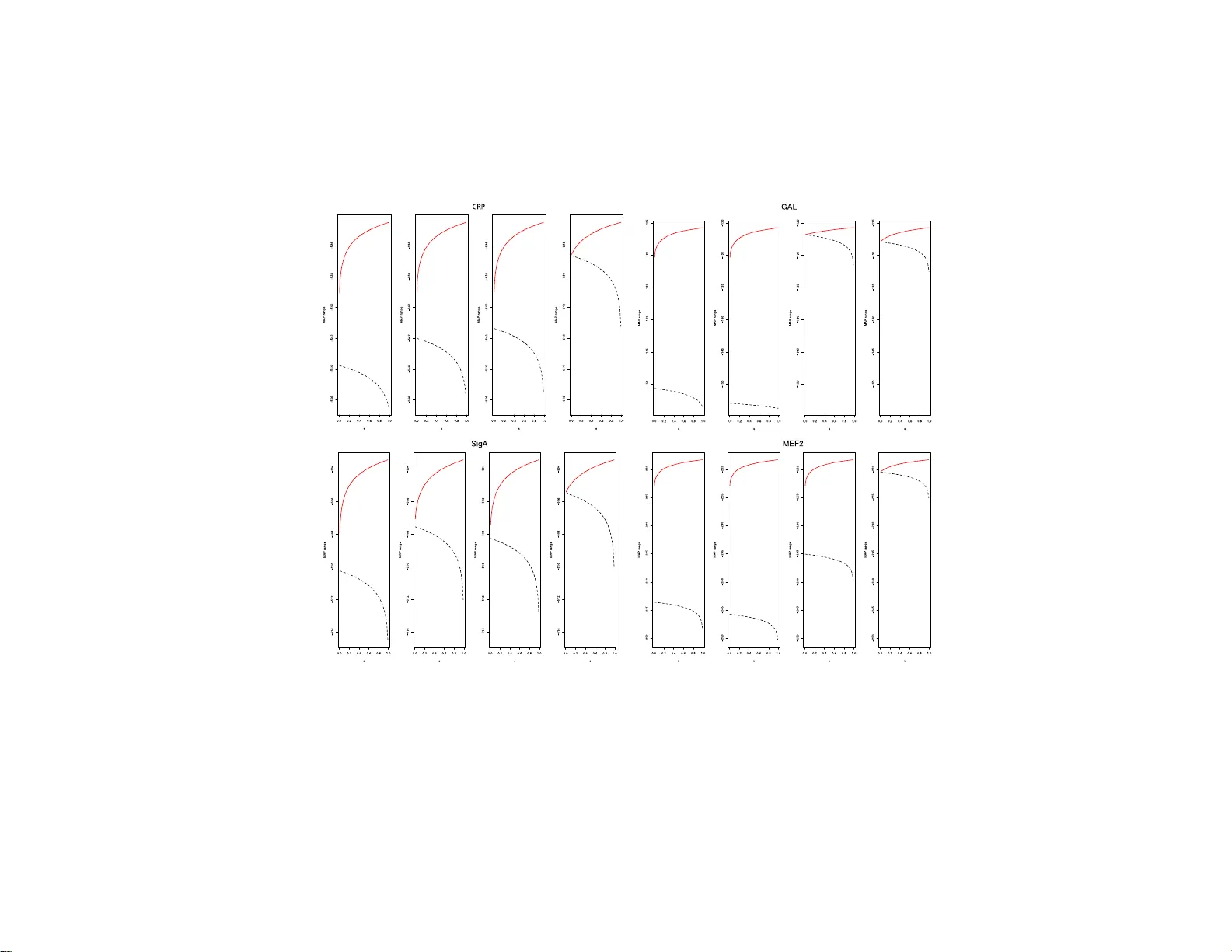
IMS Collectio ns Beyond P arametr ics in Interdisciplinary Resear c h: F estsc hrift in Honor of Professor Pranab K. Sen V ol. 1 (2008) 390– 407 c  Institute of Mathematical Stat istics , 2008 DOI: 10.1214/ 193940307 000000301 Mo d el selecti on a nd sen sitivit y analysis for sequen ce p attern mo d els ∗ Ma y etri Gupta 1 University of North Car olina at Chap el Hil l Abstract: In this article we propose a maximal a p osteriori (MAP) criterion for model selection in the motif disco v ery problem and inv estigate conditions under which th e MAP asymptotically gi ves a correct prediction of mo del size. W e also in ve stigate robustness of the MAP to pr ior specification and provide guidelines for choosing pr ior h yper- parameters for motif mo dels based on sen- sitivity considerations. 1. In tro duction: statistical c halleng es in motif disco v ery Genome sequenc ing pro jects hav e led to a rapid growth of da tabases of ge no me sequences for DNA, RNA and pro teins . The task of extracting insight in to gene reg- ulatory netw orks fr o m these mas sive amounts of da ta represents a ma jor scientific challenge. A first step tow a rds understanding the pro cess of gene r egulation is the ident ification of shor t recurr ing patterns (ab out 8-20 nucleotides long), called mo- tifs, in a set of bio -p olymer sequences. Motifs corr esp ond to functionally impo r tant parts of molecules, such as the sites wher e cer tain proteins, called transc r iption fac- tors (TFs) bind, to control gene expression. In spite of a plethora of computatio nal metho ds developed to addres s the pr oblem of motif discov er y (Sandve and Drablos [ 15 ] and Gupta and Liu [ 7 ]), most approaches still suffer from a lack of spec ific ity in motif predictions- yie lding a hig h num b er of false pos itives that a ppea r to ha ve no known biolog ical s ig nificance. T hus, one of the fundamen tal q ue s tions that arise is whether the patterns dis cov ered from the seq ue nc e data by an algorithm ar e real. Although c o nfirming the biolo gical relev a nce o f these findings often requires further biolo gical exp erimentation, it is at least imp or tant to assess their statis- tical significa nce. W e appro ach this q uestion of mo del selec tio n from a Bay esian viewp oint, us ing a n analytical approximation to the Bay es fa ctor– the maximal a po steriori (MAP) sc o ring criterion. As an ev aluation o f its p erforma nce, it is shown that the MAP a symptotically attains sev eral desira ble pr op erties. Since the Bay es factor or any such Bayesian model se lection criterio n necess arily inv olv es pa ram- eters o f the prior distribution, we also conduct sensitivity analys es to judge the effect of prior para meter sp ecifications on po sterior inference and pres crib e ro bust hyperpara meter choices for pra ctitioners. ∗ Supported by an IBM junior faculty a w ard from the Universit y of North Caroli na at Chapel Hill. 1 Departmen t of Biostatistics, 3107C McGa vran Greenberg CB# 7420, Chap el Hill, NC 27599- 7420, USA, e-mail: gupta@bi os.unc.ed u AMS 2000 subje ct classific ati ons: Pr i mary 62F15, 62P10; secondary 62F12. Keywor ds and phr ases: Bay es factor, MAP, model selection, motif disco v ery. 390 Mo del sele ction for se quence p atterns 391 1.1. Bayesian sto chastic dictionary mo del for se quenc e p atterns F or conv enience, we view the sequence data as a single sequence S = { x 1 x 2 . . . x n } of length n . S is as sumed to b e g enerated by the conca tenation o f words fro m a dictionary D of size D, where D = { M 1 , M 2 , . . . , M D } , sampled randomly accor ding to a proba bilit y vector ρ = ( ρ ( M 1 ) , . . . , ρ ( M D )). The likelihoo d of S is (1.1) P ( S | ρ ) = X Π N (Π) Y i =1 ρ ( S [ P i ]) = X Π D Y j =1 ρ ( M j ) N M j (Π) , where Π = ( P 1 , . . . , P k ) is a par tition of the s equence so that each part P i corre- sp onds to a word in the dictiona ry , N (Π) is the tota l num ber of par titions in Π, and N M j (Π) is the num ber o f o ccurrence s of word M j in the partition. Assume that the first b ( b < D ) words in the dictionary are the single letters (for DNA, b = 4 letters, { A, C, G, T } ). L e t ρ = ( ρ 1 , . . . , ρ D ) denote the word usage pr ob- abilities for the s et of all words in the dictionary . If the partition Π = ( P 1 , . . . , P k ) of the sequence into w o rds w ere known, the resulting distribution of co unts of words N = ( N 1 , . . . N D ) T would b e multinomial characterized by the proba bil- it y vector ρ . Supp ose we have D − b motifs (words other than single letters ) of widths w b +1 , . . . , w D . In the sto chastic dictionary framework, “words” M j , ( j = b + 1 , . . . , D ) are s to chastic ma trices denoted by { Θ b +1 , . . . , Θ D } = Θ ( D ) . F or the k th word of width w k , its probability matr ix is repre s ent ed as Θ k = ( θ 1 k , . . . , θ w k k ), each of the w k columns giving the pro babilities of o ccur r ence of the four le tter s at that p osition o f the word. When multiple o ccurrences of word k ar e aligned, the letter counts in the j th aligned column, c j k = ( c 1 j k , . . . c bj k ) T , ( j = 1 , . . . w k ), are characterized b y the pr obability v ectors θ j k = ( θ 1 j k , . . . , θ bj k ) T ( j = 1 , . . . w k ), of a pr o duct multinomial mo del. The count matrices corresp onding to the motifs are denoted as { C b +1 , . . . , C D } = C . The pa rtition v ar ia ble Π ca n b e equiv alently expresse d by the motif site indica- tors, denoted as A = { A ik ; i = 1 , . . . , n, k = b + 1 , . . . D } , where A ik = 1 (0) if i is the start of a s ite co rresp onding to mo tif type k (otherwise). The co mplete data likelihoo d then is : L ( N , C , A | Θ ( D ) , ρ ) ∝ Q D l =1 ρ N l l Q D k = b +1 Q w k j =1 Q b i =1 θ ij k c ijk . W e assume a Diric hlet prior distr ibution for ρ , ρ ∼ Diric hlet( β 0 ) , β 0 = ( β 01 , . . . β 0 D ), and a corres p o nding pr o duct Dirichlet prior (i.e., indep endent priors over the columns) PD( B ) for Θ k = ( θ 1 k , . . . , θ w k k ) , ( k = b + 1 , . . . D ). A Dirichlet prio r is a natural choice for this application, mo deling the join t prior densities of pro p o rtions, and is co njugate with the lik eliho o d, le ading to easy computation of the p osterior densities. Let B = ( β 1 , β 2 , . . . β w k ) be a b × w k matrix with β j = ( β 1 j , . . . β bj ) T . The co nditional p oster ior distribution o f Θ k | N , C ∝ Q w k j =1 Q b i =1 θ c ijk + β ij ij k , which is pro duct Dirichlet PD( B + C k ), the pseudo -count par ameters B b eing up dated by the column counts of the k th word, C k = ( c 1 k , . . . c w k k ). The conditional po sterior of ρ | N , C is Dirichlet( N + β 0 ) ∝ Q D l =1 ρ N l + β 0 l l . Bay es estimates of O − = ( Θ , ρ ) may b e obtained thr ough a DA pro cedure using the conditional distri- butions P ( A | O − , S ) and P ( O − | S , A ), using tec hniques of dynamic progr a mming (DP) (Gupta a nd Liu [ 6 ]). 2. Mo del se lection in the mo tif discov ery problem A tr aditional mo del selec tio n appro ach is to use likeliho o d-based criteria, for in- stance, p enalized likelihoo ds. Two wide ly used criteria a re the (i) AIC (Ak aik e’s 392 M. Gupta Information Criterion) and (ii) BIC (Bay esian Infor mation or Sc hw a r z Criterion). Leroux [ 12 ] proved that, under mild co nditions, the estima to r o btained with the nu mber of co mpo nents selected using AIC or BIC in mixture mo dels is consistent for the true mixing distribution, and has in the limit at lea st as many components. In particula r examples, howev er, it has b een o bserved that the AIC and BIC do no t give identical results: in our case, the BIC may heavily p enalize lo nger motifs, when the da ta set size is large. An alternative for judging the degree of conse r v ation o f a motif is the K ullback-Leibler infor mation criterio n (KLI), that measures the “en- tropy” distance of the motif from the background: K LI = P w i =1 P q j =1 ˆ θ ij log ˆ θ ij θ 0 j . As the exact lik eliho o d c an b e calculated computationally , using the procedure men tioned in Gupta and Liu [ 6 ], it is poss ible to calc ulate any of the a b ov e cr iteria. How ever, the dep endence structure in the sequence mo dels , when the p osition of motif sites is unknown, makes it difficult to accur ately determine the s ample siz e n for BIC. Also, the KLI is sensitive to the width of the motif- ma king it difficult to co mpa re the v alues acr oss different mo tif widths. The relative p er formance of several of these mo del selection criteria on exp erimentally verified models for rea l data sets ar e given in Section 2.4 . 2.1. The B ayesian appr o ach W e c an alternatively for mulate the q uestion as a B ay esian mo del s election problem. In the simples t s c enario, it is of interest to assess whether the seq ue nc e data sho uld be explained by mo del M 1 , which ass umes the existence of a single nontrivial motif, or M 0 , which says that the sequences are g enerated ent irely from a background mo del (e.g ., an i.i.d. or Mar ko v mo del). The Bayes facto r , which is the ratio o f the marginal likelihoo ds under the tw o mo dels, can b e computed a s p ( S | M 1 ) p ( S | M 0 ) = P A R O − p ( A , S , O − | M 1 ) d O − R O − p ( S , O − | M 0 ) d O − (2.1) = P A p ( A , S | M 1 ) p ( S | M 0 )  ≡ c 1 c 0  . The individual additive ter ms in the nu merator , after int egrating out O − , co nsist of ratios of pro ducts o f gamma functions. T o e v aluate this sum exhaustively over all partitions involv es pro hibitive amounts of computatio n. W e thus need to resor t to either Monte Car lo or some appr oximations. It can b e observed that p ( S | M 1 ) is the normalizing constant of p ( A | S , M 1 ) = p ( A , S |M 1 ) p ( S |M 1 ) = c 1 q ( A | S , M 1 ), (say) where p ( A , S | M 1 ) is of known form. Compu- tational appr oximations to estimate normalizing co nstants is a sub ject of muc h recent resea rch e.g. Meng a nd W ong [ 13 ], Chen and Shao [ 3 , 4 ], Chib and Jelia zko v [ 5 ]. W e tested imp or ta nce and bridge sampling (Meng and W ong [ 13 ]) metho ds for estimating the ratio, which ar e p o s sible to implemen t since w e can obtain MCMC draws from p 1 ( A | S ). How ever, neither metho d per forms well in most of the appli- cations, probably since the MCMC chain is extremely stic ky and hence the dr aws do not well repr esent the true distribution. The high concentration of the density of A ar ound the mo de mo tiv ates us to s eek a meas ure of significance that uses the mo dal informa tio n, a nd such a method is next dis cussed. Mo del sele ction for se quence p atterns 393 2.2. The MA P appr oximation to the Bayes factor An obvious lower bo und for ( 2.2 ) is p ( A ∗ , S | M 1 ) /p ( S | M 0 ), where A ∗ is the maximizer of the r atio. W e demonstrate how this low er b ound, called the maximal a p osteriori scor e (denoted by MAP( A ∗ )), can b e used as a mo del selectio n criterion. Definition 1. The Ma ximal a Posteriori (MAP) score under the sto c hastic dictio- nary mo del M 1 with a single motif of width w and d letters at the “b est” alignmen t A ∗ , co mpared to the background mo del M 0 (with alphab et size d ) is given b y M AP ( A ∗ ) = P ( S , A ∗ | M 1 ) P ( S | M 0 ) = p 1 ( S , A ∗ ) p 0 ( S ) . (2.2) Let c = P w j =1 c j denote the word matr ix column c ounts, N [1: d ] = { N 1 , . . . , N d } the letter freq uenc ie s and β 0[1: d ] = { β 01 . . . , β 0 d } the prio r pseudo -counts for the d letters, β 0 denoting the pseudo-c ounts for the entire set of D words ( D = d + 1 for 1 long word). Then (2.3) M AP ( A ∗ ) = R Θ , ρ 1 Q d +1 i =1 ρ N i ( A ∗ , M 1 ) 1 i Q w j =1 Q d k =1 Θ C jk ( A ∗ , M 1 ) j k p ( ρ 1 , Θ ) d ρ 1 d Θ R ρ 0 Q d i =1 ρ N i ( M 0 ) 0 i p ( ρ 0 ) d ρ 0 , where N ( · ) and C ( · ) denote the word counts and motif column counts r esp ectively , as defined in Section 1.1 . F or any indica tor vector A (repr esenting the sampled motif lo cations), we can int egrate out O − and obta in log p ( A , S | M 1 ) p ( S | M 0 ) = log  Γ( N + β 0 ) Γ( | N + β 0 | ) Γ( | β 0 | ) Γ( β 0 )  − log ( Γ( N [1: d ] + c + β 0[1: d ] ) Γ( | N [1: d ] + c + β 0[1: d ] | ) Γ( | β 0[1: d ] | ) Γ( β 0[1: d ] ) ) + w X j =1 log  Γ( c j + γ ) Γ( | c j + γ | ) Γ( | γ | ) Γ( γ )  . When ther e are D − d > 1 motifs (nontrivial sto chastic words) in the dictio nary , the logar ithm o f the MAP score (deno ted logMAP) c an be computed as: logMAP( A ) = log  Γ( N + β 0 ) Γ( | N + β 0 | ) Γ( | β 0 | ) Γ( β 0 )  − log ( Γ( N [1: d ] + c + β 0[1: d ] ) Γ( | N [1: d ] + c + β 0[1: d ] | ) Γ( | β 0[1: d ] | ) Γ( β 0[1: d ] ) ) + D X k = b +1 w k X j =1 log  Γ( c j k + γ ) Γ( | c j k + γ | )  + D X k = b +1 w k log  Γ( | γ | ) Γ( γ )  . where now c = P D k = d +1 P w j =1 c j k , and N [1: d ] and β 0[1: d ] are the same a s ab ov e. In most simulations and actual da ta s e ts , we observed that (i) the MAP score dominates the other comp onents of the Bay es fa ctor and is often more reliable to differentiate the tw o mo dels than the a pproximated Bay es factor via imp or tance sampling and (ii) the o bserved logMAP sco re in i.i.d. data se ts (co ntaining no “true” motifs) for a ny selected alignment was a lwa ys low er than that o f the n ull alig nmen t. 394 M. Gupta 2.3. Asymptotic r esults for MAP sc ori ng W e now derive asymptotic optimality criteria for judging the p e rformance of the MAP scoring statistic a s a mo del selection criter ion. In this section, we assume that ρ 0 | M 0 ∼ Dir( α ( d ) ) and ρ 1 | M 1 ∼ Dir( β ( d +1) ), where α = ( α 1 , . . . α d ) T and β = ( β 1 , . . . β d +1 ) T . Additionally , assume that the s equence is genera ted by r andom dr aws from an alphab et o f size d according to so me arbitr a ry probabilities. Let us denote the scor e for the “tr ue” alig nmen t as M AP ( A 0 ) (so that M AP ( A ∗ ) ≥ M AP ( A 0 )). The key result for esta blishing the asymptotic optimality of the MAP criterion for mo del selection is a s fo llows. Theorem 2.1. F or m exact motif inst anc es, e ach of lengt h w , in a dataset of size N , let m N P − → c , ( c < 1 w ) , N 0 i − N 1 i m P − → k i w , and N 0 i N P − → θ 0 i , ( wher e N 0 i and N 1 i ar e the fr e quency of letter i in the b ackgr ound and motif r esp e ctively, P d i =1 k i = 1 , and P d i =1 θ 0 i = 1 . ) In other wor ds, the pr op ortion of motif se quenc e to to- tal se quenc e data tends to a c onstant ; the pr op ortion of letter i in a motif tends to a c onstant k i and the sample pr op ortions of letters appr o aches the p opulation pr op ortion. Also, let r = c log c + d X i =1 ( θ 0 i − k i cw ) log ( θ 0 i − k i cw ) − d X i =1 θ 0 i log θ 0 i − [1 − c ( w − 1)] log[1 − c ( w − 1)] . (2.4) Then, r > 0 is a ne c essary and sufficient c onditio n for M AP ( A 0 ) P − → ∞ ( as N → ∞ , m → ∞ ) at a r ate ex p onential in rN . If the conditions of Theor em 2.1 ar e satisfied, M AP ( A ∗ ), and th us a lso the Bay es factor, approa ches infinity at an exp onential rate– indicating tha t asy mptotically the MAP gives the correc t mo del judgment . F ollowing from this result, w e denote the expressio n r in Theo r em 2.1 as the MAP div ergence fa ctor, or M AP DF . Theorem 2.2. The maximum value attaine d by r in expr ession ( 2.4 ) of The or em 2.1 for fi xe d c , d and w is c log c + (1 − cw ) lo g(1 − cw ) + cw log d − [1 − c ( w − 1)] log[1 − c ( w − 1)] , attaine d for θ 0 i = k i = 1 d for i = 1 , . . . , d . It is interesting to note some sp ecia l cases wher e The o rem 2.2 holds. Case 1: Symmetric base comp osition, symmetric m otif con tribution With equal background prop ortio ns o f letters , i.e. θ 0 i = 1 d for i = 1 , . . . , d , and an equal con tribution of each base to motif k i = 1 d for i = 1 , . . . , d , the conditions of Theorem 2.2 are satisfied. The p ositiv ity condition of ex pression ( 2.4 ) reduces to c log c + (1 − cw ) log (1 − cw ) + cw log d − [1 − c ( w − 1 )] lo g[1 − c ( w − 1)] > 0 . (2.5) F ro m Theorem 2.2 it is clear that the MAP score for a motif w ith other than symmetric comp ositio n will diverge mor e slowly . Another extre me case is a “r ep e at- based” motif, comp os ed o f a single letter rep eated throughout the word. Mo del sele ction for se quence p atterns 395 Fig 1 . (a) V alues of MA P divergenc e factor ( M A P D F ) incr e ase with motif widths 2 to 50 (num- b e rs on the figur e) and values of c for “e qual c ontribution ” motif, i.e. an exact motif in which e ach of the d letters o c curs the same numb er of times. (b) V alues of M AP D F for motif widths 2 to 50 and p ossible values of c for a “r e p e at-b ase d” motif. R ep e at motifs sc or e lower than motifs with e qual b ase c omp osition. Case 2: Symmetric base comp osition, “rep eat” mo ti f With equal background pro p ortions of letters, i.e. θ 0 i = 1 d for i = 1 , . . . , d , a nd a r ep e at motif: e.g ., k 1 = d ; k i = 0 for i > 1, the co nditio n in ( 2.4 ) reduce s to c log c + 1 d log d +  1 d − dcw  log  1 d − dcw  − [1 − c ( w − 1)] lo g[1 − c ( w − 1)] > 0 . (In this case, cw is neces sarily < 1 d 2 .) It is interesting to observe that a r ep eat motif will sco re lower than a motif pa ttern with a more v aried representation of letters (Panel (b) of Figur e 1 ) when all o ther parameters r emain the same. Next, we chec k how these conditions pe rform in practice for g iven c and w . More precisely , we chec k the po sitiveness of the MAP divergence factor ( M AP DF ). E xcept for very low widths ( w < 5), the M AP DF is almost a lwa ys positive (indicated in Figure 1 ), suggesting that the p erformanc e o f the MAP score a s a mo del selection criterion should improv e with increasing motif width, which is also o bserved in empirical studies. Figure 1 shows a comparatively low er v alue of M AP DF for each w , and a slower increase with w for a rep eat-ba sed motif. In bo th cases M AP DF increases with incr ease in motif prop or tion c , though the increa se is far more marked for the motif with equal ba se comp osition. 2.3.1. Multiple motif MAP monotonic pr op erty In the pr ogress ive up dating metho d that is us e d to include new motifs in to the dic- tionary , a new motif is judged to be “significa nt” based on the increas e in the MAP score after including the new motif. In this section we show that asymptotically , the MAP score monotonically increases with the size of the true dictionary , hence the MAP differ en c e cr iterion theoretica lly tends to include “true” motifs. Let us define M AP k q as the MAP s c o re corresp onding to the “true” a lig nment for q word types (including d sing le letter s and q − d motifs), where the q th word has k instances in the data set. If β i > 1 ∀ i = 1 , . . . , d , it is trivia l to show that M AP 0 q < M AP l q − 1 ∀ l > 0 , 396 M. Gupta which means that if no motifs of the new type q are present, the MAP score should theoretically show a decreas e. Next, we der ive conditions very similar to ( 2.1 ) which show that if the w ord type q is truly pr esent, the MAP score should increase– sp ecifically , we show that log M AP l q − lo g M AP l q − 1 P − → ∞ . Theorem 2.3 . L et m N P − → ρ q +1 , N 1 i N P − → ρ i (for i = d + 1 , . . . , q ) wher e N = P d i =1 N 1 i . Then M AP m q / M AP l q − 1 P − → ∞ (as m, N → ∞ ) at an ex p onential r ate in rN iff r > 0 , wher e r is given by: d X i =1 { ( ρ i − κ i wρ q +1 ) log( ρ i − κ i wρ q +1 ) − ρ i log ρ i } + log ρ ρ q +1 q +1 + lo g [1 − ( w − 1) ρ q +1 ] [1 − ( w − 1) ρ q +1 ] . Pro ofs of Theor ems 2.1 and 2.3 ar e g iven in the Appe ndix . 2.4. Performanc e of mo del sele ction criteri a F or empirica l comparisons , we used four da ta sets: CRP (S. cerevisia e or yeast), GAL4 (yeast), σ A ( B. subtilis ), and skeletal muscle TF MEF2 (hu man) (W asserma n et al. [ 17 ]). The v alue o f the MAP divergence factor ( M AP DF ) in Theo rem 2.1 is shown in Figur e 2 , for motifs in the 4 data s ets. The M AP DF is calculated for motif co mpo sition fre quency k = ( k 1 , . . . , k b ) matching that of the co nsensus mo tif (Columns 5 to 8 in T a ble 1 ). F or all mo tif o ccurrence pr op ortions c , it app ears that the M AP DF exceeds zero for the 3 data sets with lo nger motifs, viz. GAL4, CRP and MEF2 – whic h gives an indication that the conse nsus motif is likely to b e ev aluated s ignificant (under the co nditio ns of Theo rem 2.1 ). F or σ A (with lowest motif width of 6), the v alue of M AP DF is slightly b elow zero for very s ma ll c , indicating that finding the true motif may b e mor e difficult. Fig 2 . V alues of M AP D F against motif pr op ortion c for 4 data sets: (1) CRP (2) GAL4 (3) 2 motifs co rr e sp onding to σ A binding sites in B. subtilis and (4) MEF2 in human se q uenc es. w denotes the like ly width of the motif b ase d on exp e rimental data. ( σ (1) A denotes the motif “ TATAAT ” and σ (2) A denotes “ TTGACA ”.) Mo del sele ction for se quence p atterns 397 The MAP w as also compared to sev eral likelihoo d- ba sed criter ia in terms of mo del selection p erfor mance by using the knowledge o f exp erimentally detected motifs for these da ta se ts . If we s et our stopping decis ion r ule to b e s election o f motifs that keep the lo gMAP score p ositive, this co ntains the set of a ll tr ue motifs, for every data set, with an increase d power o f discriminatio n with increasing mo tif length, which ag rees with our theoretica lly obtained results. The pe rformance o f the BIC dra stically worsens when the motif length increas e s- p erhaps beca use of the higher p enalty for the increas ed num ber of para meters in the mo del. An ob jection that may b e ra ised on using the MAP for mo del selection is that it involv es the e v aluation of a “mo dal” v alue instead o f a mor e typical Bay esian quantit y inv olving a sample from the p opulation. A sample-ba sed statistic is often desirable in order to incorp or ate the p oster ior v ar iability of the distribution into the measure used. There ar e tw o main r easons why we prefer the use of the MAP score. First, the a nalytical intractabilit y of the Ba yes factor for ces us to choose an alternative approach – either computational o r analytica l. Second, it is difficult to get a “go o d” r epresentativ e poster ior sample fro m the distribution of interest i.e. p ( A | S , O − j , M 1 ), hence the lack o f a “g o o d” mean estimate. The contribution of the MAP to the BF incre ases a s the likelihoo d surfa c e b ecomes mor e s piky (hence resulting in the MAP scor e providing a b etter appr oximation) and simultaneously , the computationa l estimates for the BF ar e lik ely to p erfor m w orse, as it is mor e difficult to obtain a true re pr esentativ e sample from the distributio n. 3. Sensitivity analysis for pri or influe n ce on the MAP criterion In a B ay esian analysis, it is of co ncern to chec k the r obustness o f po sterior infer- ences to the prior specifica tion. Even asymptotically , Bay es fa c tors rema in sensitive to the choice o f prior , even tho ug h p o sterior means may not (K ass [ 8 ]). Conjugate priors are not a uto matically robust as the tails are typically o f the same for m as the likelihoo d function, and the prior remains influen tial when the lik eliho o d function is concentrated in the prior tail (Berg er [ 2 ]). With a large dimensional par ameter space, w e need to rely on the conjug a te form o f the prior for analytical and compu- tational tractability . How ever, it is still o f interest to see the influence of the choice of prior parameter s within this class on the p oster ior inferences, and develop an idea of situations leading to highes t po sterior robustness. F or investigating p o ste- rior r obustness ov er a class of priors , it is attra ctive to cons ider the ǫ - contamination class (Berge r [ 2 ]), defined by , Γ = { π : π = (1 − ǫ ) π 0 + ǫq ; q ∈ Q} , where π 0 is the original pr ior and Q r epresents an y set of distributions to ensure that Γ contains a plausible set of priors. Supp ose the p o sterior distr ibutions π 0 ( θ | x ) a nd q ( θ | x ) exist (they do for a conjugate cla ss Q ), and m ( x | π 0 ) = R θ f ( x | θ ) π 0 ( θ ) dθ a nd m ( x | π ) are the ma rginals obtained by int egrating out θ with resp ect to the prior s π 0 ( · ) and π ( · )). It is straightforward to see that π ( θ | x ) = λ q,ǫ ( x ) π 0 ( θ | x ) + [1 − λ q,ǫ ( x )] q ( θ | x ), where λ q,ǫ ( x ) = (1 − ǫ ) m ( x | π 0 ) m ( x | π ) . It also fo llows that (3.1) E π ( θ | x ) = λ q,ǫ ( x ) E π 0 ( θ | x ) + [1 − λ q,ǫ ( x )] E q ( θ | x ) . How ever, p oster io r inference based on the MAP is affected, as the MAP inv olv es the margina l likelihoo d instead of the co nditional p osterior . Let M AP q,ǫ ( A ∗ ) = P π ( S | A ∗ , M 1 ) P π ( S | M 0 ) = R O − P π ( S | A ∗ , M 1 , O − ) π ( O − ) d O − R O − P π ( S | M 0 , O − ) π ( O − ) d O − . 398 M. Gupta If we are only interested in the effect of the pr ior π ( Θ ) for the motif co lumn fre- quencies, the MAP for the co ntamination class Γ reduces to M AP q,ǫ ( A ∗ ) = R O − P π ( S | A ∗ , M 1 , O − ) π ( O − ) d O − P ( S | M 0 ) = (1 − ǫ ) M AP π 0 ( A ∗ ) + ǫM AP q ( A ∗ ) . (3.2) 3.1. Sensitivity analysis for Di richlet pri or for motif c omp osi tion γ Let us denote δ = ( δ A , . . . , δ T ) as the pseudo co unt vector for the Dirichlet distri- bution q ( γ ). Also , let δ ∗ = δ A + δ T . F o r simplicity , we assume that δ A = δ T = δ ∗ 2 , δ C = δ G = 1 − δ ∗ 2 . Then b y v ar ying 0 < δ ∗ < 1, w e get a range of c on- tamination dis tributions q . F or ǫ ∈ (0 , 1), we ev aluate the r o bustness of prior π 0 , through the v ariability in magnitude of the poster ior criter ia in ( 3.1 ) and ( 3.2 ) ov er ∆ = { δ ; 0 < δ ∗ < 1 } . Since we do not wan t the prior to dominate the data, we restrict the total pseudo count frequency P 4 j =1 δ j = 1. W e assume a single motif of width w with observed frequency ma tr ix C . Let ˆ θ ij = E ( θ ij | C ). Then, ( 3.1 ) gives ˆ θ ij = λ q ( x ) c ij + γ ij P 4 k =1 ( c ik + γ ik ) +[1 − λ q ( x )] c ij + δ ij P 4 k =1 ( c ik + δ ik ) 1 ≤ i ≤ w ; 1 ≤ j ≤ 4 . = 1 P 4 j =1 c ij + 1   c ij + γ j + ( δ j − γ j )    1 + 1 − ǫ ǫ w Y i =1 4 Y j =1  Γ( c ij + γ j ) Γ( c ij + δ j )       . Comparative studies w ere done separately to tes t the sensitivity o f the (1 ) Dirichlet prior para meters β for word frequency a nd (2) pro duct Dirichlet prior parameters γ for the column frequencies, as θ and Θ are p osterio r indep endent. Nucleotide comp osition in biolo gical sequences are often as ymmetric, e.g. a rela tively higher frequency of C/G is obser ved for higher org a nisms. With k nown motif PWMs we study the effect on p oster ior inference when we use prior s with ps eudo count frequen- cies reflecting (1) uniform le tter freque nc y (2) data comp osition-dep endent letter frequencies or (3) a mixture with co mpo nent s having different letter fr equencies. Since we a re mainly interested in whether the c onsen sus motif sequence is af- fected by the ch oice o f pr ior we s tudy the v a riation of the highest freq uency in each c o lumn ˆ θ ∗ i = max 1 ≤ j ≤ 4 { ˆ θ ij } . Co rresp onding to each choice of δ , we hav e a vector of maximal frequencie s ˆ θ ∗ δ = ( ˆ θ ∗ δ 1 , . . . , ˆ θ ∗ δ w ). Let ¯ θ ∗ δ i = 1 | ∆ | P δ ˆ θ ∗ δ i denote the mean fr equency for column i ( i = 1 , . . . , w ). T o summarize this information ov er all c o lumns we calculate three distance-based measur es, for each δ ∈ ∆ and ǫ ∈ (0 , 1)–(i) Mean squared distance: D δ M = 1 w P w i =1 h ˆ θ ∗ δ i − ¯ θ ∗ δ i i 2 , (ii) Kullback- Leibler distance: D δ K = P w i =1 ˆ θ ∗ δ i log ˆ θ ∗ δ i ¯ θ ∗ δ i , and (iii) Ent ropy or Information conten t: D δ E = − P w i =1 ˆ θ ∗ δ i log ˆ θ ∗ δ i . All three measures D M , D K and D E exhibit little v ariability , only after the third decimal place (plots not shown), slig ht ly increa sing with the co nt amination r ate ǫ . How ever, the MAP scores , calculated fo r the equa l, data-dep endent, 3-comp one nt and 9-comp onent mixture prior indicate that using the mixture prior distribution makes the MAP most robust to the choice of prior (Figure 3 ). So if the results are Mo del sele ction for se quence p atterns 399 Fig 3 . R ange in variability of MAP sc or e (in lo g sc ale on vertic al axis, may exclude an additive c onstant) at differ ent levels of prior co ntamination, for data set s (1) CRP (2) GAL4 (3) σ A (T A T AA T motif ) (4) MEF2 for human skeletal muscle data set. The four p anels for e ach data set co rr esp ond t o taking the initial prior (i) Dirichlet with symmetric b ase pseudo c ounts (ii) Dirichlet with pseudo co unts pr op ortional to fr e quency in data (iii) 3-co mp onent mixtur e Dirichlet (iv) 9 c omp onent mixtur e D i richlet. The horizontal axis on e ach plot r epr esents t he c ontamination pr op ortion ǫ . 400 M. Gupta T a ble 1 Motif and b ackgr ound letter fr e quenc ies for the 4 data sets TF Background Motif KL A C G T A C G T distance CRP 0.3021 0.1825 0.2090 0.3063 0.2841 0.1799 0.2140 0.3220 0.0011 GAL4 0.3116 0.1914 0.1761 0.3208 0.1218 0.3908 0.2983 0.1891 0.2218 σ A (T A T AA T) 0.3511 0.1465 0.1781 0.3243 0.4583 0.0699 0.0343 0.4375 0.1449 MEF2 0.2205 0.2801 0.2715 0.2278 0.6047 0.0174 0.0262 0.3517 0.6531 to b e ev alua ted using the MAP scor e at the mo de, it se e ms to b e safest to use a prior of Dirichlet mixtures instead of a sing le density . The most dramatic difference is observed in the GAL4 a nd MEF2 data o n using a mixture Dirichlet prior– these are also the da ta sets having the low est compo s itional similarity b etw een the mo tif nu cleotide frequency and background nucleotide fr e quency (K ullba ck-Leibler dis - tance in the las t column of T able 1 ). It is probable that the usual D A and the Gibbs sampler tend to pick up motifs that ar e clos er in comp os itio n to the ba ckground for a similar reason. Using a mixture Dirichlet prior ma y be more sensitive towards detecting motifs that are v a ry comp ositiona lly fr o m the bac kground. 3.2. L o c al sensitivity anal ysis One pro ble m in do ing a car eful robustness s tudy in a high-dimensional pro blem is the limitation to mainly one t ype o f high-dimensional prior distribution (the con- jugate prior) for whic h a na lytical c a lculations are feasible. An alter native approach to judge sensitivity is to lo ok for prior inputs tha t sharply change the p os ter ior answers. Such lo c al sensitivity analysis metho ds have b een extensively developed and studied by Leamer [ 11 ] and Polasek [ 14 ]. In o ur framework, we obser ve that the p oster ior mea ns are lo ca lly insensitive. Let µ j = E ( ρ j | S , A ) = N j + β j P D k =1 ( n k + β k ) . Then, ∂ µ j ∂ β i = P k 6 = i ( n k + β k )  P D k =1 ( n k + β k )  2 ≤ 1. A s imilar result holds for p oster ior mea ns of Θ . How ever, parameter sp ecifications for b oth γ and β may have a lo cal impact on the MAP . Excluding co nstant terms, and using Stirling’s approximation [ 1 ] to expand and simplify the Γ - functions, we hav e ∂ logMAP ∂ γ j ≈ X i  log c ij + γ j P k ( c ik + γ k ) − 1 2  1 c ij + γ j − 1 P k ( c ik + γ k )  + w  log P k γ k γ j − 1 2  1 P k γ k − 1 γ j  . So the influence of γ j can b e unbounded only for the seco nd term– it incr eases with w and a s the r atio of P k 6 = j γ k to γ j increases. If P k γ k = 1, the second term is w  log 1 γ j + 1 2 γ j − 1 2  , which can b e ma de arbitr a rily large if γ j is small. Under the restriction that P k γ k = 1, we will get most r obust res ults if the comp onents of γ are approximately eq ua l. W e may also do a similar a nalysis for the lo cal influence o f the prio r para meter s for ρ , i.e. fo r β . Again, we a ssume ther e is only 1 motif type under the motif model Mo del sele ction for se quence p atterns 401 (index is D ). If we differentiate logMAP with resp ect to β k , k < D , we g et log  N 1 k N 0 k  + 1 2  N 1 k − N 0 k ( N 1 k + β k )( N 0 k + β k )  + log " P D − 1 j =1 ( N 0 j + β j ) P D j =1 ( N 1 j + β j ) # + lo g " P D j =1 β j P D − 1 j =1 β j # + 1 2 P D − 1 j =1 N 0 j − P D j =1 N 1 j − β D h P D j =1 ( N 1 j + β j ) i h P D − 1 j =1 ( N 0 j + β j ) i + 1 2 1 P D − 1 j =1 β j − 1 P D j =1 β j ! , (3.3) where N 1 and N 0 are the frequencies under the motif ( M 1 ) and null ( M 0 ) mo dels. Let L denote the total length of the data . Then, L = P D − 1 j =1 N 0 j = P D − 1 j =1 N 1 j + wN D , and P D j =1 N 1 j = L − N D ( w − 1). If β D < P D − 1 j =1 β j , the influential pa rt is: 1 2 N D ( w − 1) − β D  L + P D − 1 j =1 β j − N D ( w − 1) − β D   L + P D − 1 j =1 β j  − log " 1 − N D ( w − 1) − β D L + P D − 1 j =1 β j # . Now, N D ( w − 1) < L . So if β D < P D − 1 j =1 β j , the influence of β k is s e en to be negligible for k < D . O n the o ther hand, if β D > P D − 1 j =1 β j , then the influence of the thir d, fo urth and fifth terms in ( 3.3 ) may be unbounded, but this is an unre a listic parametriza tion in practice, as the mo tif pro po rtion is usually low co mpared to the size of the data. Finally , taking deriv atives of logMAP with resp ect to β D , w e hav e, log " N D + β D P D j =1 ( N 1 j + β j ) # − 1 2 P D − 1 j =1 ( N 1 j + β j ) ( N D + β D ) P D j =1 ( N 1 j + β j ) + log 1 + P D − 1 j =1 β j β D ! + 1 2 1 β D − 1 P D j =1 β j ! . The only influential term is the third, and the influence of β D can b e unbounded if P D − 1 j =1 β j >> β D . So ideally , we wan t β D < P D − 1 j =1 β j , but also that the difference is not extremely small. In other words, results ar e most ro bust to the choice o f β D when motif prop ortions a re comparatively large. Having prio r knowledge of the true motif frequency would make it easier to get more acc urate results– by choosing β D to give the exp e c ted motif fr e q uency close to the prior knowledge. In pr actice, the choice of β D is seen to hav e a g r eat impact on motif detection a nd ev a luation, a nd this remains one o f the g reatest s tum bling blo cks of this probabilistic framework. 4. Discussion and conclusio ns A MAP cr iterion is pr o p osed for mo del selec tio n in the motif discov ery pro blem. Analytical and computational investigations es ta blish co nditions for the the MAP criterion to a symptotically pre dict the corr ect num be r of motifs a nd attaining these 402 M. Gupta conditions is se e n to b e feasible in a real scenario. W e investigate the s ensitivity of the MAP c r iterion to prio r specificatio n a nd provide guidelines for choosing these hyper-para meters to maximize robustness. The MAP is seen to p er form well as a mo del selection c r iterion in preliminar y studies, paving the w ay for further analysis of its p erfor mance when adapted to more complex realistic mo dels. App endix A: Outline o f pro o f for Theorem 2.1 F ro m expr ession ( 2.3 ), we hav e M AP ( A 0 ) ≈ Q d i =1 ( N 1 i + β i − 1 ) N 1 i + β i − 1 2 ( N 1 ,d +1 + β d +1 − 1 ) N 1 ,d +1 + β d +1 − 1 2 Q d i =1 ( N 0 i + α i − 1 ) N 0 i + α i − 1 2 ×  P d i =1 [ N 0 i + α i ] − 1  P d i =1 [ N 0 i + α i ] − 1 2  P d +1 i =1 [ N 1 i + β i ] − 1  P d +1 i =1 [ N 1 i + β i ] − 1 2 × w Y i =1 Q d j =1 Γ( c ij + γ j ) Γ  P d j =1 [ c ij + γ j ]  × k ( α, β , γ ) , where k ( α, β , γ ) =  P d +1 i =1 β i − 1  P d +1 i =1 β i − 1 2  P d i =1 α i − 1  P d i =1 α i − 1 2 × Q d i =1 ( α i − 1 ) α i − 1 2 Q d +1 i =1 ( β i − 1 ) β i − 1 2 × Γ  P d j =1 γ j  Q d i =1 Γ( γ j ) . Denote P d j =1 c ij = N 1 ,d +1 = m , P d i =1 N 0 i = P d i =1 N 1 i + mw = N ⇒ P d +1 i =1 N 1 i = N − ( w − 1) m . Then, M AP ( A 0 ) ≈ k ( α, β , γ ) × d Y i =1  1 + β i − 1 N 1 i  N 1 i + β i − 1 2  1 + α i − 1 N 0 i  N 0 i + α i − 1 2 × ( m + β d +1 − 1 ) m + β d +1 − 1 2 d Y i =1 N N 1 i + β i − 1 2 1 i N N 0 i + α i − 1 2 0 i ×      1 + P d i =1 α i − 1 N ! N + P d i =1 α i − 1 2 N N + P d i =1 α i − 1 2 × 1 + P d +1 i =1 β i − 1 − ( w − 1) m N ! N − ( w − 1) m + P d +1 i =1 β i − 1 2 × N N − ( w − 1) m + P d +1 i =1 β i − 1 2    × w Y i =1 Q d j =1 ( c ij + γ j − 1 ) c ij + γ j − 1 2  m + P d j =1 γ j − 1  m + P d j =1 γ j − 1 2 . (A.1) Mo del sele ction for se quence p atterns 403 Let the symbol ∼ = denote “ equal in order of conv ergence”, i.e. ignoring terms that conv erge to a constan t in the limit, a s N → ∞ , N 0 i → ∞ , N 1 i → ∞ . Also, as m → ∞ , m N P − → c . Then, taking lo garithms, expressio n ( A.1 ) ∼ = d X i =1 ( β i − α i ) + d X i =1 α i − 1 + d +1 X i =1 β i − 1 2 ! log [1 − c ( w − 1)] + " ( w − 1) m + d X i =1 α i − d +1 X i =1 β i # log N − w ( d − 1) 2 log 1 + P d j =1 γ j m ! +  m + β d +1 − w ( d − 1) + 1 2  log m + d X i =1  log N N 1 i + β i − 1 2 1 i − lo g N N 0 i + α i − 1 2 0 i  + e β d +1 − 1 − [1 − c ( w − 1)] N log[1 − c ( w − 1)] + w X i =1 d X j =1  c ij + γ j − 1 2  log c ij + γ j − 1 m + P d j =1 γ j − 1 ! , (A.2) since 1 − ( w − 1) m + P d +1 i =1 β i − 1 2 N ! N P − → [1 − c ( w − 1)] N → 0 (same for limit in m ). Under the conditions of the s tatement, N 0 i → ∞ , N 1 i → ∞ , N 0 i − N 1 i m P − → k i w, N 0 i N P − → θ 0 i . No w, assume that the motif is “ex act”, i.e. c ij = m for some j , every i . Now let us denote γ + = max 1 ≤ j ≤ d γ j , γ − = min 1 ≤ j ≤ d γ j . Then, the last term of ( A.2 ) is grea ter than w  m + γ − − 1 2  log( m + γ − − 1 ) ∼ = N wc log c + w  cN + γ − − 1 2  log N . (A.3) T aking the limits of a ll non-c onstant terms in expre ssion ( A.2 ), and simplifying, we then hav e log M AP ( A 0 ) ∼ = " d X i =1 ( θ 0 i − k i cw ) log ( θ 0 i − k i cw ) − d X i =1 θ 0 i log θ 0 i + c lo g c − [1 − c ( w − 1)] log[1 − c ( w − 1)] # N +   wγ − − w d X j =1 γ j − 1 2   log N . (A.4) So a sufficient c ondition for M AP ( A 0 ) P − → ∞ a t an exp onential rate is c log c + d X i =1 ( θ 0 i − k i cw ) log ( θ 0 i − k i cw ) − d X i =1 θ 0 i log θ 0 i − [1 − c ( w − 1)] log [1 − c ( w − 1)] > 0 . (A.5) 404 M. Gupta Now w e will show that ( A.5 ) actually is a necessa ry condition. Assume that condi- tion ( A.5 ) is not satisfied. If the first term in ( A.4 ) is < 0, then log M AP ( A 0 ) → −∞ . If the fir st ter m is zero, using ( A.3 ), we see that, log M AP ( A 0 ) ≥   wγ − − w d X j =1 γ j − 1 2   log N , and (A.6) log M AP ( A 0 ) ≤   wγ + − w d X j =1 γ j − 1 2   log N . In ( A.6 ), the co e fficie nt of log N is nega tive. Thus, a s N → ∞ , M AP ( A 0 ) is b ounded by 0. So condition ( A.5 ) is also a ne c essary co ndition for M AP ( A 0 ) → ∞ . App endix B: Outline of pro of for Theorem 2.2 Using the La grangia n metho d with the r estrictions ( P d i =1 θ 0 i = 1) and ( P d i =1 k i = 1), we get θ 0 i = k i = 1 d as the optimal solution. T o verify that this is the maximum v alue, le t F ( θ 0 , k ) = d X i =1 ( θ 0 i − k i cw ) log ( θ 0 i − k i cw ) − d X i =1 θ 0 i log θ 0 i . Then, ∂ 2 F ∂ θ 2 0 i = 1 θ 0 i − k i cw − 1 θ 0 i > 0, ∂ 2 F ∂ k 2 i = c 2 w 2 θ 0 i − k i cw > 0, and ∂ 2 F ∂ θ 0 i ∂ k i = − cw θ 0 i − k i cw < 0. The determinant o f the Hess ia n matr ix is k H k =    ∂ 2 F ∂ a ∂ k    =     A B B K     , where A = diag ( A i ); ( A i = ∂ 2 F ∂ θ 2 0 i ), B = diag ( B i ); ( B i = ∂ 2 F ∂ θ 0 i ∂ k i ) and K = diag ( K i ); ( K i = ∂ 2 F ∂ k 2 i ). Hence k H k = | A || K − B A − 1 B | = | A || diag ( M i ) | , where M i = c 2 w 2 θ 0 i − k i cw − c 2 w 2 ( θ 0 i − k i cw ) 2 × 1  1 θ 0 i − k i cw − 1 θ 0 i  = cw θ 0 i − k i cw  cw − θ 0 i k i  < 0 . Hence, k H k is neg ative definite, and the expr ession in ( 2.5 ) cor resp onds to the maximum attained by F . App endix C: Outline of pro of for Theorem 2.3 Let n deno te the sum of word freque nc ie s under mo del M q , i.e. n = P d i =1 N 1 i . Let m b e the num ber of word instances o f type q + 1 and l be the corr esp onding num ber of type q , q ≥ d where the alpha bet size is d a s previously . Ideally , if mo del M q +1 is true, when n → ∞ , with N q +1 n → ρ q +1 , log M AP q +1 − lo g M AP q → ∞ ; while Mo del sele ction for se quence p atterns 405 log M AP q +1 − lo g M AP q → 0 (or is b o unded ab ov e) when N q +1 n = 0. By definition, log M AP m q +1 − lo g M AP l q = log   Q q +1 i =1 Γ ( N 2 i + β i ) Γ  P q +1 i =1 β i  Γ  P q +1 i =1 [ N 2 i + β i ]  Q q +1 i =1 Γ( β i )   − lo g  Q q i =1 Γ ( N 1 i + β i ) Γ ( P q i =1 β i ) Γ ( P q i =1 [ N 1 i + β i ]) Q q i =1 Γ( β i )  + log   w Y i =1 Q d j =1 Γ( c ij k + γ j ) Γ  P d j =1 Γ[ c ij k + γ j ]    + w log   Γ  P d j =1 γ j  Q d j =1 Γ( γ j )   , (where k = q + 1 − d ) . (C.1) If N 2 ,q +1 N = 0, then in ( C.1 ), N 1 i N − N 2 i N → 0 for i ≤ q . Then ( C.1 ) b eco mes log[Γ ( P q +1 i =1 β i )] − log[Γ( P q i =1 β i )] − log Γ( β q +1 ) = log Beta ( P q i =1 β i , β q +1 ). A s uf- ficient co nditio n for log M AP q +1 − log M AP q < 0 is β q +1 > 1, P q i =1 β i > 1. Now we derive the monotonicity pr op erty of the MAP score, i.e. when N q +1 N → ρ q +1 , un- der mo del M q +1 , lo g M AP q +1 − log M AP q → ∞ . Leaving out the co ns tant ter ms, ( C.1 ) reduces to log   Q d i =1 Γ( N 2 i + β i )Γ ( N 2 ,q +1 + β q +1 ) Γ ( P q i =1 [ N 1 i + β i ]) Q d i =1 Γ( N 1 i + β i )Γ  P q +1 i =1 [ N 2 i + β i ]    + w X i =1 log   Q d j =1 Γ( c ij k + γ j ) Γ  P d j =1 c ij k + P d j =1 γ j    . Let us denote m = N 2 ,q +1 = P d j =1 c ij k ∀ i = 1 , . . . , w . Then P q i =1 N 2 i + mw = P q i =1 N 1 i = n . Using Stirling’s a pproximation, ( C.1 ) reduces to d X i =1  N 2 i + β i − 1 2  log ( N 2 i + β i − 1 ) −  N 1 i + β i − 1 2  log ( N 1 i + β i − 1 )  −  m + β q +1 − 1 2  log ( m + β q +1 − 1 ) + q X i =1 [ N 1 i + β i ] − 1 2 ! log q X i =1 [ N 1 i + β i ] − 1 ! − q +1 X i =1 [ N 2 i + β i ] − 1 2 ! log q +1 X i =1 [ N 2 i + β i ] − 1 ! + w X i =1   d X j =1  c ij k + γ j − 1 2  log ( c ij k + γ j − 1 ) −   m + d X j =1 γ j − 1 2   log   m + d X j =1 γ j − 1     , (C.2) 406 M. Gupta since, for i = d + 1 , . . . , q , we have N 1 i = N 2 i . Leaving out constants and ter ms tending tow ards 0 a s N 1 i → ∞ , N 2 i → ∞ , we ca n wr ite ( C.2 ) as d X i =1  N 2 i + β i − 1 2  log ( N 2 i ) −  N 1 i + β i − 1 2  log ( N 1 i )  +  m + β q +1 − 1 2  log ( m + β q +1 − 1 ) + n + q X i =1 β i − 1 2 ! log  1 + P q i =1 β i − 1 n  − " n − ( w − 1) m + q +1 X i =1 β i − 1 2 # log " 1 − ( w − 1) m + P q +1 i =1 β i + 1 n # +[ m ( w − 1) − β q +1 ] log( n ) + w X i =1   d X j =1  c ij k + γ j − 1 2  log ( c ij k + γ j − 1 ) −   m + d X j =1 γ j − 1 2   log   m + d X j =1 γ j − 1     . (C.3) Now we ev aluate eac h of the terms as n → ∞ , m → ∞ , with m n P − → ρ q +1 . Assume that the prop ortion contributed to motif ( q + 1) b y each ba se i, i = 1 , . . . , d is κ i , such that N 1 i − N 2 i m P − → wκ i , i = 1 , . . . , d , P d i =1 κ i = 1 and, as b efore, n − mw = P q i =1 N 2 i . Also, as sume that all instances of the motif are exact, i.e. c ij k = m for some j ∈ 1 , . . . , d ∀ i = 1 , . . . , w . Also, for a ll i, j , let γ ( i ) = γ j if c ij k = m . So, finally , simplifying terms in ( C.3 ), we g et, n " d X i =1 { ( ρ i − κ i wρ q +1 ) log( ρ i − κ i wρ q +1 ) − ρ i log ρ i } +[1 − ( w − 1) ρ q +1 ] log[1 − ( w − 1 ) ρ q +1 ] + ρ q +1 log ρ q +1 # + n log n [ − w + 1 + w − 1] ρ q +1 + lo g n   w X i =1 γ ( i ) − w d X j =1 γ j   . (C.4) Let r denote d X i =1 { ( ρ i − κ i wρ q +1 ) log( ρ i − κ i wρ q +1 ) − ρ i log ρ i } + ρ q +1 log ρ q +1 + [1 − ( w − 1) ρ q +1 ] log[1 − ( w − 1 ) ρ q +1 ] . Then ( C.4 ) P − → ∞ at a rate exp onential in r n iff r > 0. If r = 0, the c o efficien t of log n , P w i =1 γ ( i ) − w P d j =1 γ j ≤ 0 so lo g M AP q +1 − log M AP q P − → 0. Also, by a similar ar gument as in T heo rem 2.2 , the maximum v alue is attained when κ i = ρ i = 1 d , for i = 1 , . . . , d . Ac knowledgmen ts. The author is g rateful to Jun S. Liu for helpful comment s. Mo del sele ction for se quence p atterns 407 References [1] Abramowitz, M. and Stegun, I. A. (1972). Handb o ok of Ma thematic al F unctions . Dover, New Y or k. [2] Ber ger, J. O. (1993 ). St atistic al De cision Th e ory and Bayesian A nalysis . Springer, Berlin. MR12344 89 [3] Chen, M. -H. and Shao, Q.-M. (19 97a). E s timating ratios of no rmalizing constants for densities with different dimensio ns. Statist. Sinic a 7 607 –630 . MR14674 51 [4] Chen, M.-H. and Sha o, Q.-M. (199 7b). On Monte Ca rlo methods for estimating ratios of nor ma lizing co nstants. Ann. S t atist. 25 1563 –159 4. MR14635 65 [5] Chib, S . and Jeliazkov, I. (200 1). Mar ginal likelihoo d from the Metrop o lis- Hastings output. J. Amer. Statist. Asso c. 96 2 70–28 1. MR1952 737 [6] Gupt a, M. and Liu, J. S. (2003). Disco v ery of cons e r ved sequence pat- terns using a sto chastic dictionary mo del. J. Amer. Statist. Asso c. 98 55–66 . MR19656 74 [7] Gupt a, M. and Liu, J. S. (20 0 6). Bayesian mo deling and inference for motif discov ery . Bayesian Infer en c e for Gene Expr ession and Pr ote omics . Cambridge Univ. Press . [8] Kass, R. E. (1993). Bayes factors in practice. Statistician 42 551 –560. [9] La wrence, C. E., Al tschul, S. F., Boguski, M. S., Liu, J. S., Neuw ald, A. F. and Wootton, J. C. (19 93). Detecting subtle sequence sig nals: A Gibbs sampling stra tegy for multiple alignment. Scienc e 262 20 8–14. [10] La wrence, C. E. and Reill y, A. A. (1990). An exp ectation-ma ximization (EM) a lgorithm for the identification and characterization of co mmon sites in biop olymer sequences . Pr oteins 7 4 1–51 . [11] Leamer, E. E. (1982). Sets of p oster ior means with bounded v ariance prior . Ec onometric a 50 7 2 5–73 6. MR06627 28 [12] Leroux, B. G . (1 992). Co nsistent estimation of a mixing distribution. A nn. Statist. 20 13 50–13 60. MR1186253 [13] Meng, X . L. an d Wong, W. (1996). Sim ulating ratios o f normalising con- stants via a simple identit y: A theoretica l exploration. Statist. Sinic a 6 831– 860. MR14224 06 [14] Polasek, W. (1982). Local sensitivity analysis and ma trix deriv atives. In Op er ations R ese ar ch in Pr o gr ess (G. F e ichtin ger et al., eds.) 425–44 3. Reidel, Dordrech t. MR0710 505 [15] Sandve, G. K. and Drablos, F. (2006). A survey of motif discovery meth- o ds in an integrated fra mework. Biolo gy Dir e ct 1 11. [16] Stormo, G. D. and H ar tzell, G. W. (1989 ). Identifying protein-binding sites from unaligned DNA fragments. Pr o c. Natl. A c ad. Sci. USA 86 1183– 1187. [17] W asserman, W. W ., P al umbo, M., Thompson, W., Fickett, J. W . and La wrence, C. E. (2000). Human-mouse genome comparis ons to lo cate regulator y sites. Natu r e Genetics 26 2 25–22 8.