Projected likelihood contrasts for testing homogeneity in finite mixture models with nuisance parameters

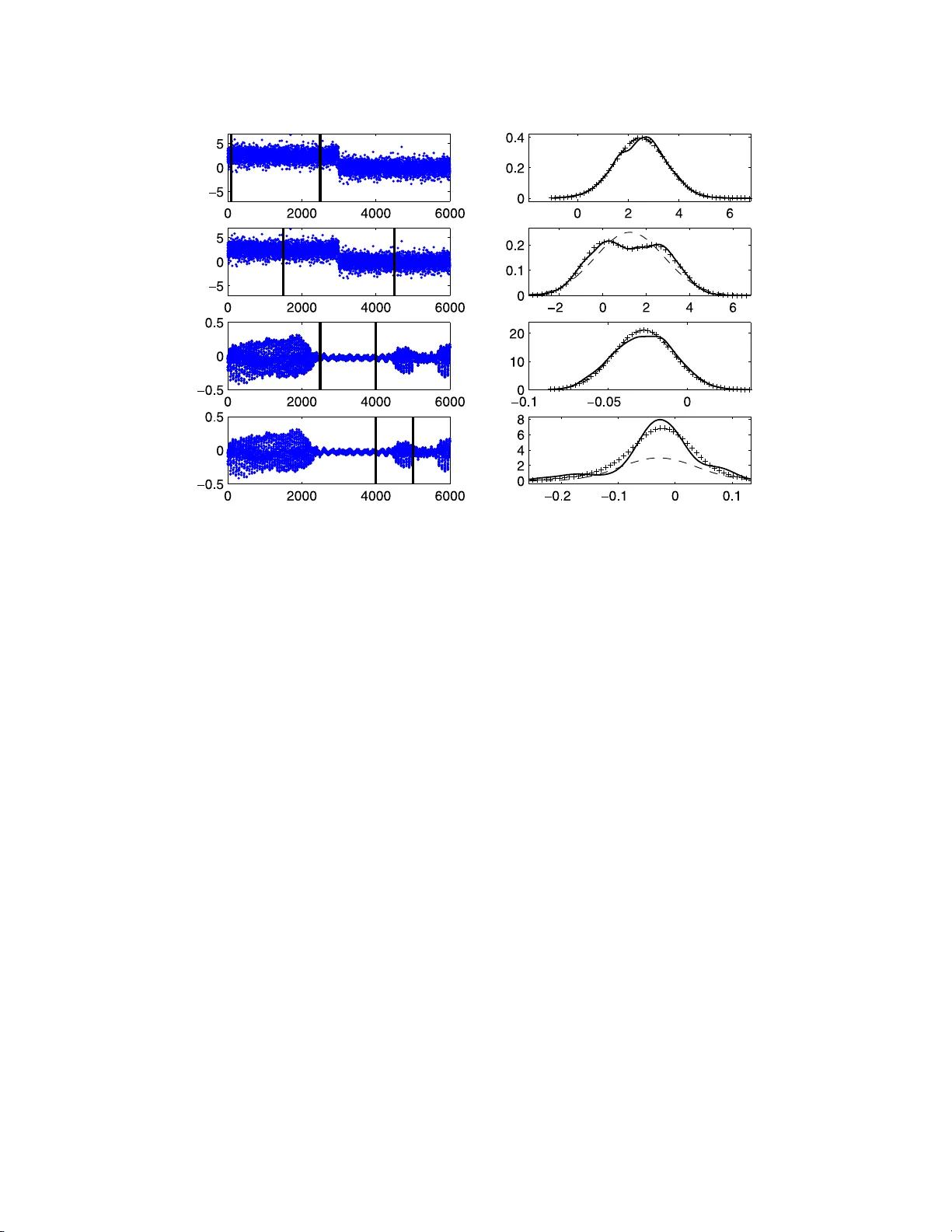
IMS Collectio ns Beyond P arametr ics in Interdisciplinary Resear c h: F estsc hrift in Honor of Professor Pranab K. Sen V ol. 1 (2008) 272– 281 c  Institute of Mathematical Stat istics , 2008 DOI: 10.1214/ 193940307 000000194 Pro jected lik e liho o d con trasts for testing homogene i t y in fin i te mixture mo dels with n uisance p arameters Debapriy a Sengupta ∗ 1 and Rah ul Mazumder 2 Indian Statistic al Institute Abstract: This paper dev elops a test for homog eneit y in finite mixture mod- els where the mixing proportions are kno wn a priori (tak en to b e 0.5) and a common n ui sance pa rameter is presen t. St atistical tests based o n the no- tion of Pro jected Like liho o d Contrasts (PLC) are considered. The PLC is a slight modification of the usual likelihoo d ratio statistic or the Wilk’s Λ and is similar i n spir it to the Rao’s score test. Theoretical inv estigations hav e been carried out to understand the l arge sample statistical prop erties of these tests. Simulation studies hav e b een carried out to understand the b ehavior of the n ull distribution of the PLC statistic i n the case of Gaussian mi xtures with unkno wn m eans (common v ari ance as n uisance parameter) and unkno wn v ari - ances (common mean as nuisance parameter). The results are i n conformity with the theoretical results obtained. Po we r functions of these tests hav e been ev aluated based on simulations from Gaussian mixtures. 1. In tro duction Finite mixture mo dels are o ften used to understand whether the data comes from a heterog eneous or a homo geneous p opula tion. In pa rticular, consider the case of a mixture of tw o p opulations with the mixing pr op ortions known (Goffinet et al. [ 7 ]). W e are in terested to know whether the data is sampled from a prop er mixture of tw o distributio ns o r a single distribution. In particular , c o nsider a mixtur e family g , with g enerating po pulation densities given by M 0 = { f ( ·| θ, η ) : θ ∈ Θ , η ∈ E } , where θ is the main para meter of interest and η is the co mmon nuisance par ameter. W e as sume tha t the mixing prop ortio n is known a prio ri to b e 0 . 5. The mixture mo del then b ecomes (1.1) g ( z | θ 1 , θ 2 , η ) = 0 . 5 f ( z | θ 1 , η ) + 0 . 5 f ( z | θ 2 , η ) . The null hypothes is fo r homogeneity is, θ 1 = θ 2 . In several pr a ctical examples (for exa mple, ar ising in sp eech ana lysis and non- parametric regressio n metho dology) detection of the lo cation of disc ontinuity in the lo c a l mean or the lo ca l v a riance (or lo ca l amplitude) are of interest (Figure 1). The theoretica l r esults developed in this pap er can b e use d in such problems. Fig- ure 1 demonstrates several sc e narios of s ignals b e ing sca nned through a running ∗ Supported in part by Gran t No. 12(30)/04-IRSD, DIT, Govt . of India. 1 Ba ye sian and Int erdisciplinary Research U nit, Indian Statistical Institute, 203 B. T. Road, Kolk ata 700108, India, e-mail: dps@isic al.ac.in 2 C. V. Raman Hall , 205 B. T. Road, Kolk ata 7001 08, India, e-m ai l: rahul.ma zumder@gm ail.com AMS 2000 subje ct classific ati ons: Pr i mary 62G08, 60G35; secondary 60J55. Keywor ds and phr ases: Gaussian mixture mo dels, pro j ected likelihoo d contrast. 272 Pr oje cte d likeliho o d c ontr asts 273 Fig 1 . L eft c olumn shows time plots of data with solid vert i c al lines marking the windows co n- sider e d. The top two p anels indic ate a simulate d noisy signal (with additive Gaussian noise) with me an function having a jump disc ontinuity. The b ottom p anels describ e a p ortion of digitize d sp e e ch waveform. In the right c olumn thr e e fitte d densities of y - values: nonp ar ametric kernel smo othe d density (solid line), single c omp onent Gaussian fit (dashe d line) and mixtur e of two Gaussian fit with e qual mixing weights (curve indic ate d by + ), ar e shown c orr esp onding to the fr ames indic ate d in the left c olumn. window of sp ecified bandwidth. When the c ent er o f the window is pla c ed at p o in ts of discontin uit y the r aw signal v alues ( y -axis) will hav e a distribution which can be adequately mo deled by ( 1.1 ). This bas ic idea has b een explo red by Hall and Titterington [ 8 ] in the context of edg e a nd p ea k preserving smo others . A brie f list of r eferences dea ling with the study of mixture distributions and prop erties of the Likeliho o d Ratio T est (LR T) tests a re pr ovided b elow. In Tit- terington et al. [ 13 ], McLachlan and Ba sford [ 11 ] and Lindsay [ 1 0 ] o ne may find extensive discus s ions ab out the background o f finite mixture mo dels. The a symp- totic distr ibutions of the LR T in mixture mo dels have b een studied in Bickel a nd Chernoff [ 1 ], Chernoff and Lander [ 5 ], Ghosh and Sen [ 6 ], Lemdani and Pons [ 9 ]. Different mo difications o f LR T tests in mixture mo dels a re pro p o sed and studied by Chen et al. [ 4 ] and Self and Lia ng [ 12 ]. In this pap er we introduce a co ncept of Pro jected L ikeliho o d Contrasts (PLC), a mo dified version of the LR T test o r the Wilks’ Λ (Wilks [ 14 ]) statistic, which we motiv ate as follows. Consider i.i.d. obse rv ations Z 1 , Z 2 , . . . , Z N generated by some element of the class of densities g given by ( 1.1 ). The likelihoo d under the full mixture mo del is g iven by (1.2) L N ( θ 1 , θ 2 , η ) = N X i =1 log g ( Z i | θ 1 , θ 2 , η ) , where g is defined through ( 1 .1 ). Under the null hypothesis the likelihoo d reduces 274 D. Sengupta and R. M azumder to the usual likeliho o d under M 0 , na mely , (1.3) L N ( θ, θ, η ) = N X i =1 log f ( Z i | θ, η ) . Define ( ˆ θ , ˆ η ) a s the maximum likelihoo d estimator s of ( θ , η ) under ( 1.3 ). The idea behind the PLC statistics is to plug in the estimated nuisance para meter under the nu ll in ( 1.2 ) and maximize it ov er remaining para meters θ 1 and θ 2 . Finally the PLC statistic is defined a s (1.4) Λ N = 2  max θ 1 ,θ 2 L N ( θ 1 , θ 2 , ˆ η ) − L N ( ˆ θ, ˆ θ , ˆ η )  . The term pro jected likelihoo d is us ed here to distinguish the pro cedure from pr o file likelihoo d. W e call it pr o jected likeliho o d b ecause the profile of the nuisance par am- eter is o btained a fter pro jecting the full likelihoo d onto f ( ·| ˆ θ, η ) ∈ M 0 . That wa y we first obtain a pr o jected profile of η a nd then maximize it so that its estimate coincides with the ma ximum likelihoo d estimate (MLE ) under the null hypothesis. Note that this pr o cedure, in spirit, is very similar to the Rao ’s score test. The pap er is org anized as follows. In Sectio n 2, the larg e sa mple prop erties of the P LC statistics is discussed. In Sec tion 3, some simulation studies a r e provided. The pro of of the main theorem in Section 2 is provided in the Appendix. 2. Large sample appro ximation of PLC statis tic F or the purp ose of theoretical inv e s tigation we shall simplify the mo del further a s - suming that the cla s s of densities are all one dimensio nal. Denote the null h ypo thes is by (2.1) H ∗ 0 : Z 1 , Z 2 , . . . , Z N are iid M 0 F or notational conv enience we adopt the conv ention that the symbol D r x indicates r -th partial deriv ative with res pe c t to x , treated a s a generic a rgument in a function. Define the following es timated scor e s (2.2) ˆ ξ r ( j ) = D r θ f ( Z j | ˆ θ N , ˆ η N ) f ( Z j | ˆ θ N , ˆ η N ) , for 1 ≤ j ≤ N and r ≥ 1. Analo g ously define the true scores ξ r ( j ) = D r θ f ( Z j | θ ,η ) f ( Z j | θ ,η ) at the true parameter v alues under H ∗ 0 . One can verify that E H ∗ 0 ξ r (1) = 0 fo r every r ≥ 1 in case of reg ular pa rametric families. Note that under regula rity assumptions on the model the sco res a re well b ehav ed and ha ve finite momen ts. F or the Gaussian case all moments will b e finite since the joint mo ment g enerating function of any finite set of p olynomia ls inv olving ξ r ’s exists. Define the following mixed partia l der iv atives of the full likelihoo d L N . (2.3) C N ij = ( D θ 1 + D θ 2 ) i ( D θ 1 − D θ 2 ) j L N ( ˆ θ N , ˆ θ N ) , where i, j ar e nonnegative integers. Moreov er, let ¯ C N ij = N − 1 C N ij . Although the quantities defined in ( 2.3 ) lo o k quite inco mprehensible they ca n how ever b e ex- pressed as linea r co mbinations o f D l θ 1 D m θ 2 L N ( θ 1 , θ 2 ) us ing the Binomial e xpansion. Pr oje cte d likeliho o d c ontr asts 275 One can esta blis h with some effor t the following. D i θ 1 D j θ 2 log g ( z | ˆ θ N , ˆ θ N , ˆ η N ) = P Ω ∗ a (Ω) Q i + j r =1 ˆ ξ ω r r ( z ) , where P ∗ runs ov er all nonnega tive in tegral partitions Ω = ( ω 1 , ω 2 , . . . , ω p + q ) satisfying P r ω r = i + j . The co efficients a (Ω) are compli- cated combinatorial q uantities but can b e r ecursively computed. It can be verified that C N ij = 0 if j is o dd. W e provide simplified expressio ns for some of the lower order C N ij which are necessa r y for future calculations. (2.4) ¯ C N 20 = 1 N P N j =1 ( ˆ ξ 2 ( j ) − ˆ ξ 2 1 ( j ) ) ( P → −I ) , ¯ C N 02 = 1 N P N j =1 ˆ ξ 2 ( j ) ¯ C N 12 = 1 N P N j =1 ( ˆ ξ 3 ( j ) − ˆ ξ 1 ( j ) ˆ ξ 2 ( j )) , ¯ C N 04 = 1 N P N j =1 ˆ ψ ( j ) , where ˆ ψ ( j ) = ˆ ξ 4 ( j ) + 1 2 ˆ ξ 1 ( j ) ˆ ξ 3 ( j ) − 3 ˆ ξ 2 2 ( j ) + 3 ˆ ξ 2 1 ( j ) ˆ ξ 2 ( j ), and I is the Fis her information of θ under H ∗ 0 . Finally , let ¯ C ij denote asymptotic ex pe c ted v alues o f ¯ C N ij under H ∗ 0 which can be ea sily derived using Lemma 2.1 (i). T he distributional prop erties of ¯ C N ij can be derived using cla ssical prop erties of M - estimators. W e state the following lemma for the sake of completeness. The pro of can b e found in Bick el and Doksum [ 2 ]. Lemma 2.1 . L et Z 1 , Z 2 , . . . , Z N b e indep endent and identic al ly distribute d r andom variables with density f ( z | θ ) satisfying usual r e gularity c onditions with the s c or e function S ( z , θ ) and Fisher information matrix I = Cov θ ( S ( Z 1 , θ )) . (i) L et ψ ( z , θ ) b e a r e al value d, c ontinuously differ entiable (in θ ) kernel with E θ ψ 2 ( Z 1 , θ ) < ∞ , for every θ . F urt her let ˆ θ N denote the MLE of θ . Then 1 N N X i =1 ψ ( Z i , ˆ θ N ) P → E θ ψ ( Z 1 , θ ) . (ii) In addition if ψ satisfies E θ ψ ( Z 1 , θ ) = 0 for every θ then (2.5) 1 √ N N X i =1 ψ ( Z i , ˆ θ N ) = ⇒ N (0 , V 2 ) , wher e V 2 = E θ ψ 2 − C ′ I − 1 C wher e C = Cov θ ( ψ ( Z 1 , θ ) , S ( Z 1 , θ )) . Finally , we pr o ceed to the main asymptotic r epresentation theor em of the P LC statistic. It turns o ut that even in the Gaussian ca se the standar d χ 2 -approximation do es not hold. Actually it turns out that Ga ussian ca se is more paradoxical than one would exp ect. As a r esult one ha s to go for higher order expansion to get an idea of the limiting b ehavior of the statistic. The crucial issue is whether E H ∗ 0 ξ 1 (1) ξ 2 (1) = 0 or not. This is a meas ure o f s ome type of spurio us non-deg eneracy in the mo del due to skewness a nd its asy mptotic effect needs to b e corr e c ted for. Two cases are considered in the simulation section. In the fir st case we conside r a mixture Gaussia n with different means but c o mmon unknown v ariance a nd the in seco nd case sc ale mixture Gaussian with common unknown mean is consider ed. In b oth cases we find E H ∗ 0 ξ 1 (1) ξ 2 (1) = 0 . The first case is c overed by Theorem 2.2 (i) b elow while the second case is cov ered by Theorem 2.2 (ii). W e state the theorem keeping these t wo sp ecial cases in mind. The pro of of the theor em is provided in the App endix. Theorem 2.2. Assum e that E H ∗ 0 ξ 1 (1) ξ 2 (1) = 0 and C 04 < 0 . Then u nder H ∗ 0 , (i) if ¯ C N 02 = 0 , then Λ N P → 0 . 276 D. Sengupta and R. M azumder (ii) if √ N ¯ C N 02 = ⇒ N (0 , σ 2 ) for some σ 2 > 0 , then (2.6) Λ N = ⇒ c 2 max(0 , Z ) 2 , for suitable c 2 > 0 and a standar d n ormal variate Z . 3. Simulation studies in the case of Gauss ian mi xtures In this section we provide results p ertaining to the sampling distributions o f the PLC s tatistic under the null in c a se o f Gaussian mixtures [ 7 ]. Studies have bee n carried out for tw o different cas e s : unknown v a riances and common mean as the nu isance pa rameter and unknown means and common v ariance as the nu isance parameter. The simulation results ar e in c o nformity with the theor etical r esults derived. The power function of the P LC test statistic for each o f the ab ove tw o set-ups have b een studied for different v alues of the alterna tive. Simulation studies hav e b een ca rried o ut for different sample sizes. 3.1. Nul l distri butions of the PLC Consider the pa rticular exa mple of Gauss ia n mixture mo dels, the main par ame- ters of interest a re the unknown means and the common v aria nce is the nuisance parameter. The gener ating mo del is given by (3.1) f ( z | θ , η ) = η − 1 φ (( z − θ ) / η ) where φ is the standa rd normal probability density function ( θ ∈ ℜ , η > 0 ) . In this cas e ˆ η 2 = N − 1 P N i =1 ( Z i − ¯ Z ) 2 , where ¯ Z = N − 1 P N i =1 Z i . The corr esp onding PLC is denoted by Λ m N . Simulation studies for the n ull distribution of Λ m N hav e bee n p erfor med for sample sizes N = 50, 100 and 200. Percentiles of the sampling distribution a r e display ed in T able 1 which s hows how differe nt p ercentiles p (5, 50 and 95) of the null distr ibution of Λ m N decrease with increasing sample s ize N . The difference of the p er c ent ile v alues, (say that betw een p ercentiles 95 and 5), decreases with increasing s a mple siz e as well. The tabulated v alues give sufficient reason to b elieve in the v alidity of the theor etical results obtained in Theor em 2.2 . In the second exa mple, also per taining Gaus s ian mixture mo dels, the main pa - rameters of interest are unknown v aria nces and the co mmon mean is the nuisance parameter. (3.2) f ( z | θ , η ) = θ − 1 φ (( z − η ) /θ ) for θ > 0 , η ∈ ℜ . Here ˆ η = ¯ Z . The cor resp onding PLC statistic is deno ted by Λ s N . T able 1 Per c entiles of the nul l distribution of the PLC, co rr esp onding to a Gaussian mixtur e with unknown me ans and c ommon varianc e as the nuisanc e p ar ameter P ercen tiles N 5 50 95 50 0.008 0.011 0.014 100 0.004 0.005 0.006 200 0.002 0.002 0.003 Pr oje cte d likeliho o d c ontr asts 277 The co nstant c 2 in the limiting distributio n ( 2.6 ) can b e co mputed, but the computations are quite c umber some. Hence the cons tant c 2 has b e en ev alua ted based on the sampling distribution of Λ s N under the null. The sa mpling distribution is based on 5000 simulations of data- size 2000. The v alue o f c 2 hence obta ined is 0.6907 0. The a s ymptotic null distribution of Λ s N is a mixture of a deg enerate mass at 0 and a c 2 χ 2 1 (for suitable c 2 > 0), with mixing prop or tion 0.5. The sampling distri- bution of Λ s N , obtained fro m 5000 simulations of sample siz e 200 0, is found to b e a mixture of outcomes whic h are exactly zero and another s trictly p os itive abso lutely contin uo us distributio n. W e have obser ved that this absolutely co nt inuous distri- bution (as obtained from simulations) is very c lo se to c 2 χ 2 1 (where c 2 = 0 . 6907 0) as depicted in Figur e 2 . Hence sim ulation studies of the n ull distribution show sufficient confor mity to the theoretical res ults o bta ined in Theorem 2.2 . Sim ulation studies for the null distribution of Λ s N hav e b een p e rformed and tabulated (see T able 2 ) for differe nt sample sizes N ba sed o n 1 0 00 s imulations of data size N wher e N = 5 0 , 1 0 0 , 200 . The expe c ted v alue of the sa mpling distribution shows a negative bias. The degree to which it a pproximates the mean of the larg e sample distribution of the PLC improv es with increasing sample siz e. The pro p o rtion o f zer os in the sampling Fig 2 . Dotted line shows the kernel density est i mate of c 2 (max { 0 , N (0 , 1) 2 } )( c 2 = 0 . 69070) , the the or etic al asymptotic nul l distribution of the PLC under N (0 , 1) . Note that by invarianc e the r esults do not dep end on the choic e of the me an and varianc e. The solid line is t he kernel density estimate of t he sampling distribution of the PLC with the zer os left out, under the nul l c orr esp onding to a Gaussian mixt ur e of the same set -up. This sampling distribution is b ase d on 5000 simulations of sample size 2000. T able 2 Summary statistics of the nul l distribution of the PLC, co rr esp onding to a Gaussian mixtur e with unknown varianc e and c ommon me an as the nuisanc e p ar ameter Expecta tion % of zeros 5% signif. p oint N Theor.* Est. Theor. Est. Theor .* E st. 50 0.345 0.156 50 70.1 1.86 0.935 100 0.345 0.256 50 61.5 1.86 1.608 200 0.345 0.328 50 57.5 1.86 1.817 *The sampling distribution based on 5000 simulations of sample-size 2000, has b een used as a prox y for the theoretical asymptotic n ull di stribution. 278 D. Sengupta and R. M azumder Fig 3 . Solid line, dotted line and dashe d line c orr esp ond t o the sample size s 200, 100 and 50 r esp e ct ively in b oth the figur es. Power functions of the PLC t est statistic at level α = 0 . 05 have b een evaluate d. In the c ase of Λ m N , (left figur e) the p ower function has b een evaluate d for values of t he p ar ameter | θ 1 − θ 2 | 2 ∈ [0 , 2] . The p ower function c orr esp onding t o Λ s N (right figur e) has also b een evaluate d f or the values of the p ar ameter q max { θ 1 ,θ 2 } min { θ 1 ,θ 2 } ∈ [1 , 3] . distribution go es on decr e asing with N b efore it a symptotes to the theoretical v a lue 0.5. The degre e to which the sampling distribution approximates the theoretical distribution improv es with inc r easing sample size in the case o f the 95 th per centile. 3.2. Power function of the PLC test statistic Po w er functions corre s po nding to the test statistic Λ m N at level α = 0 . 05 hav e be en ev aluated for different v a lues of the par ameter (different v a lues o f the alterna tive) | θ 1 − θ 2 | 2 in the range [0 , 2] , fo r thre e different s ample s izes N = 5 0 , 100 , 200 . (Fig- ure 3 ). The p ow er is found to increase with increas ing sample size. Po w er functions corr esp onding to the test statistic Λ s N at lev el α = 0 . 0 5 have b een ev aluated for different v a lues of the par ameter (different v a lues o f the alterna tive) q max { θ 1 ,θ 2 } min { θ 1 ,θ 2 } in the range [1 , 3 ] , for three different s a mple sizes N = 50 , 100 , 2 00 . (Figure 3 ). The p ow er is found to increase with increas ing sample size. App endix: Pro of o f Theorem 2.2 First, it fo llows from Chen e t al. [ 4 ] that b oth the MLEs ˆ θ 1 and ˆ θ 2 resp ectively are N 1 / 4 consistent under ( 1.1 ). F or b oth the cases in the theore m we re- parametrize the problem with θ 1 = ˆ θ N + N − 1 / 2 s + N − 1 / 4 τ and θ 2 = ˆ θ N + N − 1 / 2 s − N − 1 / 4 τ and study its be havior near ( ˆ θ N , ˆ θ N ) in the neighbo r ho o ds | s | ≤ lo g N and | τ | ≤ log N resp ectively . In what follows we do not verify orders o f r e mainder terms explic itly . Several technical steps nee d to b e verified in the pro cess of deriving the re sult. W e refer to Bick el and Doksum [ 2 ], Ghosh and Sen [ 6 ] and Bo se and Sengupta [ 3 ] fo r the t yp e of re gularity assumptions and machinery needed for uniform approximations in such a context. Also, note that under the a b ove parametriza tion the likelihoo d bec omes an even function in τ . Therefore we work with τ ≥ 0 without a n y loss o f generality . The asymptotic pro blem is non-standar d b eca use the Fisher informa tion matrix, I ( θ 1 , θ 2 , η ), has rank 2 if θ 1 = θ 2 and 3 otherwis e (can b e verified by Pr oje cte d likeliho o d c ontr asts 279 straightforward differen tiation). Next define H ( s, τ ) = L N ( ˆ θ N + s + τ , ˆ θ N + s − τ ) . It can b e rea dily verified from ( 1.2 ) a nd ( 2 .3 ) tha t (A.1) ∂ i + j ∂ s i ∂ τ j H (0 , 0) = C N ij , for i, j ≥ 0. The strategy of the proo f is the following. Since the expansio n is re g ular in within-mo del displac ement s , we fix τ ≥ 0 and maximize over s in the first step. Then, we examine the b ehavior of the maximum v alue obtained in the firs t step across τ to derive the final res ult. Because of our g eneral reg ula rity co nditions a ll the following calculatio ns will b e v a lid uniformly in probability ov er the compact set | s | ≤ lo g N and 0 ≤ τ ≤ lo g N . I n what follows γ > 0 shall denote a gener ic constant whose v alue may be determined on a ca se by case basis. Also , in der iv ing the or ders of r emainders we specially mention one simple fact from ca lculus, namely , N − a (log N ) b → 0 as N → ∞ for a ny a, b > 0. H ( N − 1 / 2 s, τ ) = H (0 , τ ) + s [ N − 1 / 2 H 10 (0 , τ )] + 1 2 s 2 [ N − 1 H 20 (0 , τ )] + o P ( N − γ ) , (A.2) where H ij ’s denote resp ective partial deriv atives o f H . Also, it can b e chec ked that H 20 (0 , τ ) = − N I (1 + o P ( N − γ ) ) . Therefore, in la rge samples, for fixed 0 ≤ τ ≤ N − 1 / 4 log N , the maximum v alue of H ( N − 1 / 2 s, τ ) ov er the compact set | s | ≤ lo g N cannot exceed its unrestric ted global maximum, which is of the order of [ N − 1 / 2 H 10 (0 , τ )] 2 / [ N − 1 H 20 (0 , τ )]. B y direct T aylor series of or der 4 we find H 10 (0 , N − 1 / 4 τ ) = (2!) − 1 [ √ N ¯ C N 12 ] τ 2 + (4!) − 1 [ ¯ C N 14 ] τ 4 + o P ( N − γ ) . The facts r e q uired for the ab ov e s implifica tion a re: (i) H 10 (0 , 0) = 0 by the maxi- m um likeliho o d equatio n, (ii) H 1 j (0 , 0) = 0 for j o dd (since H is an even function of τ ) a nd (iii) the assumption of the theo r em that E H ∗ 0 ξ 1 (1) ξ 2 (1) = 0 . It can b e chec ked that the last as sertion implies √ N ¯ C N 12 = O P (1), in view o f ( 2.4 ) and Lemma 2.1 . Therefore b y virtue of the a ssumptions of the theo rem the profile g lobal max i- m um of H ( · , τ ) b e comes neglig ible in pr obability over the rang e of int erest. Thus we hav e (A.3) max | s |≤ log N H ( N − 1 / 2 s, τ ) = H (0 , τ ) + o P ( N − γ ) , uniformly over 0 ≤ τ ≤ N − 1 / 4 log N . Fina lly , H (0 , N − 1 / 4 τ ) = H (0 , 0 ) + (2!) − 1 [ √ N ¯ C N 02 ] τ 2 + (4!) − 1 [ ¯ C N 04 ] τ 4 + o P ( N − γ ) . Therefore we have (A.4) Λ N ≈ 2 max | s |≤ log N , 0 ≤ τ ≤ log N [ H ( N − 1 / 2 s, N − 1 / 4 τ ) − H (0 , 0)] = max 0 ≤ τ ≤ log N { [ √ N ¯ C N 02 ] τ 2 + 1 12 [ ¯ C N 04 ] τ 4 + o P ( N − γ ) } . 280 D. Sengupta and R. M azumder Now we consider case (i) of the theor e m where ¯ C N 02 = 0. Then ( A.4 ) r educes to Λ N = max 0 ≤ τ < log N { (1 / 12 ) [ ¯ C N 04 ] τ 4 + o P ( N − γ ) } . Since C 04 < 0 it follows form Lemma 2.1 that Pr { ¯ C N 04 < − δ } → 1 for arbitr arily small δ > 0. By c ho osing τ > 12 1 / 4 δ − 1 / 4 N − γ / 4 one can s how that the v alue of the o b jectiv e function (b eing maximized) b ecomes nega tive. Hence it can b e verified that Λ N P → 0. F or ca se (ii) arguing in a simila r line and collecting the do minant terms from ( A.3 ) and ( A.4 ) a nd then maximizing the dominant term with resp ect to τ (noting that the dominant expressio n is a quadratic in τ 2 and ¯ C N 04 P → C 04 ( < 0)) we obtain (A.5) Λ N ≈ max 0 ≤ τ ≤ log N { [ √ N ¯ C N 02 ] τ 2 + 1 12 [ ¯ C N 04 ] τ 4 } ≈ − 3 [max(0 , √ N ¯ C N 02 )] 2 ¯ C 04 , with an err or in approximation of the order of o P ( N − γ ) as befor e. Hence the sec o nd part of the the theorem follows from the a ssumptions. References [1] Bickel, P. J. and Chernoff, H. (199 3). Asymptotic distribution of the likelihoo d ratio statistic in a pr ototypical non regular problem. In Statistics and Pr ob ability: A Ra ghu R aj Bahadur F estschrift (J. K . Gho sh, S. K. Mitra , K. R. Parthasara th y and B. Prak asa Rao, eds.) 8 3–96. Wiley , New Y ork. [2] Bickel, P . J. and Do ksum, K. A. (200 1 ). Mathematic al St atistics . Basic Ide as and Sele cte d T opics . 1, 2 nd ed. Prentice Hall, NJ. MR04431 41 [3] Bose, A. and Sengupt a, D. (200 3). Strong consistency of minimum contrast estimators with a pplica tions. Sankhy¯ a 65 4 40–46 3. MR20289 09 [4] Chen, H ., Chen, J. and Kalbfleisch, J. D. (200 1). A mo dified likeliho o d ratio test for homogeneity in finite mixture mo dels. J. R. St at. S o c. Ser. B Stat. Metho dol. 63 1 9–29. MR18119 88 [5] Chernoff, H. and Lander, E. (1995). Asymptotic distribution o f the likeli- ho o d ratio test that a mixture of tw o binomials is a single binomial. J. Statist. Plann. In fer enc e 43 19– 40. MR13141 26 [6] Ghosh, J. K. and Sen, P. K. (1985). On the as ymptotic p erfor mance of the log likeliho o d ratio statistic for the mixture mo del and rela ted results. In Pr o c. of t he Berkeley Confer enc e in Honor of Jerzy Neyman and Jack K iefer I I (Berkeley, Calif., 1983) 78 9–806 . W adsworth, Belmont, CA. MR08220 65 [7] Goffinet, B., Loisel, P. and La urent, B. (1992). T esting in normal mixture mo dels when the prop o r tions are known. Biometrika 79 842 –846. MR12094 83 [8] Hall, P. and Titterington, D. M. (1992). E dge-prese rving a nd p eak - preserving smo othing. T e chnometrics 34 429– 440. MR1190 262 [9] Lemdani, M. and Pons, O. (19 99). Likelihoo d r atio tests in contamination mo dels. Bernoul li 5 705 –719. MR170 4 563 [10] Lindsa y, B. G. (1995 ). Mixtur e Mo dels: The ory, Ge ometry and Applic ations . Institute of Mathematica l Statistics , Hayw ard, CA. [11] McLachlan, G. J. and Basford, K. E. (1988). Mixtu r e Mo dels: In fer enc e and Applic ations to Clust ering . Dekker, New Y ork. MR09264 84 [12] Self, S. G. and Liang, K.-Y . (198 7). Asymptotic prop erties of ma ximum likelihoo d estimators and likelihoo d ratio tests under nonsta ndard co nditions. J. Amer. Statist. Asso c. 8 2 605–6 10. MR08983 65 Pr oje cte d likeliho o d c ontr asts 281 [13] Titterington, D. M., Smith, A. F. M. and Mako v, U. E . (1985). Statis- tic al Analysis of Finite Mixtur e D istributions . Wiley , Chichester. MR08380 90 [14] Wilks, S. S. (1 938). The larg e sample distribution of the likeliho o d ratio for testing comp osite hypo thes is . Ann. Math. Statist. 9 60 –62.