Statistical inference under order restrictions on both rows and columns of a matrix, with an application in toxicology

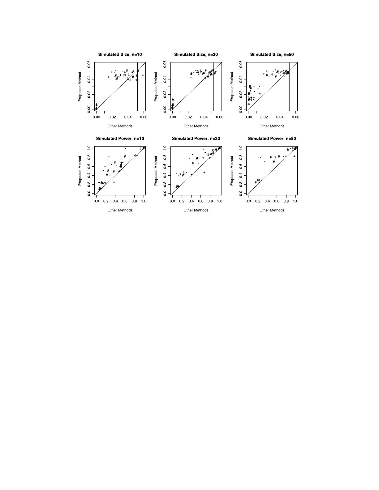
IMS Collectio ns Beyond P arametr ics in Interdisciplinary Resear c h: F estsc hrift in Honor of Pro fessor Pranab K. Sen V ol. 1 (2008) 62–77 In the Public Domain DOI: 10.1214/1 939403070 00000059 Statistic al inference un der order restrict ions on b oth rows and colu mns of a matrix, wit h an applicati on in toxicology Eric T eoh ∗ 1 , Abraham Nysk a 2 , Uri W ormser 3 and Sh y amal D. Peddada † 4 Insur anc e Institute for Highway Safety, T el Aviv University, The Hebr ew Unive rsity of Jerusalem and NIEHS Abstract: W e presen t a general met hodology for perfor ming statistical infer- ence on the components of a r eal-v alued mat rix paramete r for which ro ws a nd columns are sub ject to order restrictions. The proposed estimation procedure is based on an iterative a lgorithm deve lop ed b y Dykstra and Robertson (1982) for simple order restriction o n rows and columns of a matrix. F or any order re- strictions on rows and columns of a m atrix, sufficient conditions are deri v ed for the algorithm to con v erge i n a single application of row and column operations. The new algorithm is a pplicable to a broad collection of order restrictions. In practice, it i s e asy to de sign a st udy such that t he sufficient conditions derived in this paper are satisfied. F or instance, the sufficient conditions are satisfied in a b alanced design. Using the estimation p ro cedure developed i n this article, a b o otstrap test f or order restrictions on ro ws and columns of a matri x is pro- posed. Computer simulations for ordinal data we re p erformed to compare the proposed test with some existing test pro cedures in terms of size and p ow er. The new methodology is illustrated b y applying i t to a set of ordinal data obtained fr om a toxico logical study . 1. In tro duction In man y applica tions the para meter of interest θ can b e expressed as elements of a real-v alued I × J matr ix such that the elements w ithin rows and/or columns of the matrix ar e sub ject to inequality restrictions ca lled order r estrictions. Researchers are often in terested in dr awing statistical inferences on such parameter s sub ject to a v ariety o f or der restrictions. F or a parameter vector η = ( η 1 , η 2 , . . . , η p ) ′ , some commonly enco un tered or der restrictio ns are; simple or der , where η 1 ≤ η 2 ≤ · · · ≤ ∗ This w ork was done while the author was a summer in tern at the National Institute of En- vironment al Health Sciences (NIEHS) and a graduate studen t in the Departmen t of Biostatistics, Unive rsity of N orth Caroli na, Chap el Hill, NC, USA. † Supported b y the In tramural Research Pr ogram of the NIH, National Institute of En viron- men tal Health Sciences. 1 Insurance Institute for Highw a y Safety , Arlington, Vi rginia, USA, e-m ai l: eteoh@ii hs.org 2 T oxicologic Pathologist, T el Aviv Universit y , T el Aviv, Israel, e-mail: anyska@b ezeqint.n et 3 Departmen t of Pharmacology , School of Pharmacy , F aculty of M edicine, Institute of Life Sciences, The Hebrew Uni versity of Jerusalem, Jerusalem, Israel, e-mail: wormser@ cc.huji.a c.il 4 Biostatistics Branc h, NIEHS, Research T riangle P ark, NC, USA, e-mail: peddada@ niehs.nih .gov AMS 2000 subje ct classific ations: Primary 62F10; secondary 62G09, 62G10. Keywor ds and phr ases: linked parameters, matrix partial or der, maximally-linked subgraph, order-restriction, ordinal data, sim ple order, si m ple tree order, umbrella order. 62 Or der r estrictions on r ows and c olumns of a matrix 63 T ab le 1 F or e ach r esp onse variable, the data structur e of the exp eriment in Wormser et al. [ 26 ] Sample Leve l of skin injury Genotype size Unremark abl e Minimal Mild Mo derate Ma rked Co x-2 deficien t 10 n 1 , 1 n 1 , 2 n 1 , 3 n 1 , 4 n 1 , 5 Wild t ype 10 n 2 , 1 n 2 , 2 n 2 , 3 n 2 , 4 n 2 , 5 Co x-1 deficien t 10 n 3 , 1 n 3 , 2 n 3 , 3 n 3 , 4 n 3 , 5 η p , umbr el la or der , where η 1 ≤ η 2 ≤ · · · η i ≥ η i +1 ≥ · · · ≥ η p and simple tr e e or der , where η 1 ≤ η i , for all 2 ≤ i ≤ p . Recently W ormser et al. [ 26 ] conducted an exp eriment to ev alua te the differ- ences among three different genotypes of mice, namely , the wild type (WT), the cyclo oxygenase-1 deficien t (COX-1-d) and the cy clo oxygenase-2 deficient (COX-2- d) mice, when they were e x po sed to s ulfur m ustard (also known as mustard gas). Depending up on the severit y of injury to skin, each animal was categoriz e d into one of five ordered categor ies, namely , “unremar k able”, “minimal”, “mild”, “mo d- erate”, and “marked” (details in Section 5 ). In this exper iment, a sample of n = 1 0 animals from ea ch genotype was ex p o sed to sulfur mustard. Let n i,j , i = 1 , 2 , 3, j = 1 , 2 , . . . , 5, denote the n um be r of anima ls in the i th genotype that belong to j th resp onse category , with E ( n i,j ) = nπ i,j . Then the parameters of in terest are the cum ulative probabilities θ i,j = P j k =1 π i,k , i = 1 , 2 , 3 , j = 1 , 2 , 3 , 4 . Note that θ i, 5 = 1, i = 1 , 2 , 3. T able 1 summarizes th e type of data obtained in W ormser et al. [ 26 ]. Clearly , the rows of θ satisfy a simple order a s they represent cumulativ e probabilities. A ccording to W ormser et al. [ 26 ], CO X-2 deficiency has a protective effect a g ainst infla mma tory pro ces ses while COX -1 deficiency has a negative effect. Consequently , each column of θ is also sub ject to simple order restriction. Thus in this example the r ows as well as columns of θ are sub ject to s imple o rder r e striction. The ab ove type of matrix or der restric tio ns commo nly arise in a v ar iety co nt exts such as the analys is of ordinal data (cf. Agre s ti and Coull [ 1 ], Gro v e [ 9 ], Nair [ 16 ] and W a ng [ 2 5 ]), sur viv al a nalysis (Pr aestgaa rd [ 19 ]), Phase I clinical trials inv olving “co cktail” o f tr eatments (Conaw ay et a l. [ 6 ]) and analy sis of time-course a nd do s e- resp onse gene expr ession microarr ay s tudies, etc. F or a given parametric family with matrix v alued para meter θ ∈ Θ ⊂ R I × J , where Θ is the pa rameter space defined by order res tr ictions on the rows and/or columns of θ , one ma y estimate θ using re stricted maximum likeliho o d estimato r s (RMLEs) and test alternative hypotheses using the likelihoo d ra tio tests and their mo difications. Such metho ds hav e b een well studied in the literature (cf. Barlow et al. [ 2 ], Rob ertson et al. [ 21 ] and Silv apulle and Sen [ 23 ]). How ever, a s seen from Hw ang a nd Peddada [ 11 ] a nd Lee [ 1 2 ], the RMLE is not always efficient r elative to the unrestricted maximum likeliho o d estimator (UMLE). Also , the likelihoo d ratio tests in the pr esent co ntext may not b e computatio nally simple and the asymptotic distribution under the n ull hypothesis may involv e nuisance par ameters (cf. F ra nck [ 8 ], Gro v e [ 9 ], Robertson and W right [ 20 ] a nd W a ng [ 25 ]). Silv apulle [ 22 ] provided an interesting explanatio n for wh y sometimes the RMLEs and the likeliho o d ra tio tests provide c ounter-in tuitiv e results. In view of the g e neral concer ns rega rding RMLE and the likelihoo d ratio tests, in Section 2 we introduce a computationally stra ightf orward metho dology for estimat- ing a matrix v a lued parameter θ when the rows and/or columns are sub ject to o rder restrictions. The prop os ed estimation pro cedure is based o n the iterative pro cedur e of Dykstra and Ro ber tson [ 7 ] and uses the metho d of Hwang and Peddada [ 11 ] for general or der restrictions . If the elements of the random matrix are indep endently 64 E. T e oh et al. and no rmally dis tr ibuted and if r ows as well as columns of the matrix are sub ject to simple or der r estriction then the prop o s ed pro c edure is identical to the estimator given in Dykstra a nd Rob er tson [ 7 ], but the tw o pro cedur es may differ for other order restrictions. Using the prop osed point estimators, in Section 3 we intro duce a Kolmogo rov-Smirnov type test statistic and a bo otstr ap-based methodolo gy for determining significance. The perfor mance of th e prop osed test procedur e is ev al- uated us ing c omputer simulations in Section 4 and in Se c tion 5 it is illustrated by analyzing the data in W ormser et al. [ 26 ] mentioned above. Concluding re ma rks are provided in Section 6. 2. Estimatio n of parameters sub ject to order restrictions 2.1. Notations and a brief r eview Throughout this pap er R p denotes the vector space o f p × 1 real v ectors and R I × J denotes the v ector space of I × J real matric es. Two compo nents θ i,j and θ r,s of θ ∈ Θ ⊂ R I × J are said to b e linke d if the inequality b etw een them is known a priori . A parameter is said to b e a no dal parameter if it is linked to a ll I J c omp onents of θ ∈ Θ ⊂ R I × J . A s ubset of par ameters M , f ormed by the comp onents of θ ∈ Θ ⊂ R I × J , is a linke d s u b gr aph if all para meters in M are linked, with a t least o ne strict inequality . Note that every link ed subg r aph repr esents a simple order- restriction and conv ersely , ev ery simple o rder is a linked s ubgraph. A linked subgraph M is said to b e maximal ly linke d if for a ny linked subgraph N , M ⊂ N = ⇒ M = N . If a subset of par a meters sim ultaneously satisfies t w o linked subgraphs M a nd N , then we us e the notation M Λ N to describ e the subset. As noted in Peddada et al. [ 18 ], any o rder-r e striction betw een parameters can be expresse d in terms of a colle c tion of maximally linked subgra phs. Similarly , every para meter θ i,j app ears in a finite collectio n of maximally link ed subgraphs as a noda l par ameter (within each subgraph). Such max imally link ed subgraphs a r e said to b e asso ciate d with θ i,j . If the rows of θ ar e s ub ject to order restrictio n R ⊂ R I and the columns are sub ject to orde r restriction C ⊂ R J then we sha ll deno te the joint order restriction by R Λ C ⊂ R I × J . The notatio n R Λ R J would indicate order r estrictions R on the rows a nd no order restrictions on the columns of θ . Similarly , the notation R I Λ C would indicate order restrictions C on th e columns and no order r estrictions on the r ows of θ . It is imp or ta nt to emphas ize that in this article we only consider linked subgra phs which are subsets of rows or which are subsets of columns of the para meter θ . Thus we are not considering inequa lities betw een arbitra r y linear or non-linea r functions of the elements of θ . Example 2. 1 (Umbrella order restriction on the rows o f θ ) . Supp ose the ele- men ts of each r ow of θ are sub ject to an umbrella order with p eak in the s th column. That is, the components of the i th row of θ satisfy the inequalities θ i, 1 ≤ θ i, 2 ≤ · · · ≤ θ i,s ≥ θ i,s +1 ≥ · · · ≥ θ i,J , i = 1 , 2 , . . . , I . Then in this case the parameters o f the i th row ca n b e e x pressed in terms of t w o maximally link ed subgraphs, namely , M i, 1: s = { ( θ i, 1 , θ i, 2 , . . . θ i,s ) | θ i, 1 ≤ θ i, 2 ≤ · · · ≤ θ i,s } a nd M i,s : J = { ( θ i,s , θ i,s +1 , . . . , θ i,J ) | θ i,s ≥ θ i,s +1 ≥ · · · ≥ θ i,J } . Th us, the subse t of parameters in the i th row of θ , i = 1 , 2 , . . . , I , can be expressed as M i, 1: s Λ M i,s : J . F urther, for r ≤ s , the maximally linked subgraph asso ciated with θ i,r in the i th row, i = 1 , 2 , . . . , I , is M i, 1: s . Or der r estrictions on r ows and c olumns of a matrix 65 F or a vector x = ( x 1 , x 2 , . . . , x p ) ′ ∈ R p , a simple or der op er ator C S w : R p → S is an o rthogona l pro jection op erator on to the simple o rder c one S = { x ∈ R p : x 1 ≤ x 2 ≤ · · · ≤ x p } where w is a vector of p ositive w eights and the i th comp onent o f C S w ( x ) is given b y (2.1) ( C S w ( x )) i = min s ≥ i max t ≤ i P s j = t w j x j P s j = t w j . W e s hall use the ter minology s imple or der function to describ e the min-max fo rmula used in ( 2.1 ). Remark 2.1. F or a fixed weigh t vector w , C S w is a mono tonic op er ator in the sense that if x ≤ y then C S w ( x ) ≤ C S w ( y ), where the inequalit y is component wise. When estimating a parameter η = ( η 1 , η 2 , . . . , η p ) ′ sub ject to a rbitrary or der restrictions C ⊂ R p with at least one no da l parameter , Hw ang a nd Peddada [ 11 ] used the simple order oper ator C S w , with a suitable w eight vector w , for estimating the no dal pa r ameters. Typically the w eights are pr op ortional to the pr ecision (or sometimes the s ample size) of UMLE. Once a para meter is estimated, then the corres p o nding UMLE is replaced by the new restricted estimator and is assigned arbitrar ily la rge weigh t B , B → ∞ , in a ll subsequent ca lculations. T o estimate a non-no dal para meter, ide ntify the collection of a ll maximally linked s ubgraphs asso ciated with that non-no dal par ameter and apply the simple or de r op er a tor C S w on the v ector corresp o nding to the subgraph with a suitable w eight vector w . Suitable mo difications were prop osed for gr aphs with no no dal parameters . Example 2.2 (Um brella order r e striction) . Suppo se η is a par ameter satisfying the o rder re s triction η 1 ≤ η 2 ≤ η 3 ≥ η 4 ≥ η 5 with UMLE ˆ η . In this case the only no dal parameter is η 3 . Supp ose w = ( w 1 , w 2 , w 3 , w 4 , w 5 ) ′ is the w eight vector asso ciated with ˆ η . According to Hwang and Peddada [ 11 ] the estima tio n pro cedur e beg ins with the no da l parameter η 3 . F or i = 1 , 2, denote w ( i ) = w i , ˆ η ( i ) = ˆ η i and let w (3) = w 5 , w (4) = w 4 , w (5) = w 3 and ˆ η (3) = ˆ η 5 , ˆ η (4) = ˆ η 4 , ˆ η (5) = ˆ η 3 . Then η 3 may b e estimated by the follo wing simple order formula ˆ ˆ η 3 = max i ≤ 5 P 5 j = i w ( j ) ˆ η ( j ) P 5 j = i w ( j ) . Next, the no n-no dal parameters η 1 , η 2 , η 4 and η 5 are estimated using the maxima lly linked subgra phs η 1 ≤ η 2 ≤ η 3 and η 3 ≥ η 4 ≥ η 5 , resp ectively . The estimator s f or the non-no dal par ameters η 1 , η 2 are simplified as follows: ˆ ˆ η 1 = min { ˆ η 1 , w 1 ˆ η 1 + w 2 ˆ η 2 w 1 + w 2 , ˆ ˆ η 3 } , ˆ ˆ η 2 = min { ma x( w 1 ˆ η 1 + w 2 ˆ η 2 w 1 + w 2 , ˆ η 2 ) , ˆ ˆ η 3 } . In a similar manner η 4 and η 5 are estimated. Remark 2.2. F or a given w , C C w is a function of several simple or der functions and therefore C C w is a monotonic opera tor. That is, fo r all x ≤ y , C C w ( x ) ≤ C C w ( y ), where the inequalities a re compo nent wise . 2.2. Estimation of matrix value d p ar ameters W e extend the notations from the previous section to matrix v alued par ameters as follo ws. F or a matrix X ∈ R I × J and a w eight ma tr ix W , we denote the matrix 66 E. T e oh et al. simple or der c olumn op er ator by C S W . Each column x of X is orthog onally pro jected onto the simple o r der cone S using C S w , where w is a suitable column vector of W . Similarly , the matrix simple or der r ow op era tor is denoted by R S W , which, with rows of W , pr o jects each row vector of matrix X ∈ R I × J orthogo nally onto the s imple order cone S . Ana logously , for arbitra ry o rder r estrictions D , we define matrix column and row op erato rs using Hwang and Peddada metho dolo gy by C D W and R D W , resp ectively . W e no w describe the propo sed algorithm for estimating θ ∈ Θ = R Λ C ⊂ R I × J using an unrestricted p oint estimator ˆ θ . W e us e the weigh t matrix W R when o p- erating on the rows of ˆ θ and weigh t matrix W C when ope r ating on the columns of ˆ θ . Step 1 (An un r estr icte d estimator) : Obtain an unrestricted estimator ˆ θ for an I × J matrix parameter θ . Note that in most situations a user may prefer to sta rt with the unres tricted maximum likelihoo d estimator (UMLE), altho ugh it is not requir ed. Step 2 (Estimation under o r der r estrictions on the c olumns of θ ) : Apply the pro cedure of Hwang a nd Peddada [ 11 ] on each column of ˆ θ to obtain estimates for θ under the order-r estriction on the co lumns of θ . That is, apply t he op erator C C W C on the columns of ˆ θ and denote the resulting estimator b y C C W C ( ˆ θ ). Note that the elements of C C W C ( ˆ θ ) may no t satisfy the order-r estriction on the rows of θ . Step 3 (Estimation under o r der r estrictions on the ro ws of θ ) : Apply the op erator R R W R on the rows of C C W C ( ˆ θ ) and denote the resulting estimator by ( R R W R ◦ C C W C )( ˆ θ ). Step 4 (Iter ate to c onver genc e) : Repe a t Steps 2 and 3 to o btain the q th iterate, ( R R W R ◦ C C W C ) q ( ˆ θ ). Stop when s o me reasona ble conv ergence criterion is reached. Denote lim q →∞ ( R R W R ◦ C C W C ) q ( ˆ θ ) as ˜ θ 1 . Step 5 (Final estimate) : Since R R W R and C C W C do not necessa rily commute for all or der restrictions and weigh ts used in the calculated weight ed av erages, rep eat the pro c ess b eg inning with within-row order re s trictions follow ed by within-column order restrictio ns. That is, compute ˜ θ 2 = lim q →∞ ( C C W C ◦ R R W R ) q ( ˆ θ ). The final estimate of θ ∈ Θ is taken to be (2.2) ˆ ˆ θ ≡ 1 2 ( ˜ θ 1 + ˜ θ 2 ) . Remark 2. 3. In general ˜ θ 1 6 = ˜ θ 2 . T o illustrate this, consider the v ery spec ia l case where θ is a 2 × 2 matrix with rows and co lumns bo th sub ject to the s imple order restriction θ 1 ,j ≤ θ 2 ,j , θ i, 1 ≤ θ i, 2 , i = 1 , 2 , and j = 1 , 2. Consider the extr eme case where ˆ θ is a sy mmetr ic matrix with ˆ θ 1 , 1 ≤ ˆ θ 1 , 2 = ˆ θ 2 , 1 ≥ ˆ θ 2 , 2 . F urther, suppo se W C = W R = 11 ′ . Thus we ha ve a perfectly “symmetric” pr oblem where w e may exp ect ˜ θ 1 = ˜ θ 2 . Ho w ever, ev en in this ra ther s eemingly ob vious s ituation ˜ θ 1 6 = ˜ θ 2 , but ˜ θ 1 = ˜ θ ′ 2 . Hence the c omp osition ( R R W R ◦ C C W C ) is no t co mm utative. F or this reason, we need to in vok e Step 5 in a ll situations. Before w e discuss the conv ergence of the ab ov e algorithm in Steps 4 and 5, w e consider the following example which may be instructiv e. Or der r estrictions on r ows and c olumns of a matrix 67 Example 2.3. Consider a clinical tr ial compar ing 3 new treatments with an ex- isting treatmen t using 4 do se groups p er treatmen t g roup. F or the j th dose of the i th treatment, i, j = 1 , 2 , . . . , 4, let ˆ θ i,j denote the sample mean respo nse based on n i,j = n obser v ations. F urther, for simplicity of illustr a tion, let ˆ θ i,j ∼ indep N ( θ i,j , c ), i, j = 1 , 2 , 3 , 4. Without lo ss of gener ality , let the firs t row of θ corresp ond to the ex- isting trea tmen t. The n the order r estrictions of interest ar e θ 1 ,j ≤ θ i,j , i ≥ 2, j ≥ 1, i.e. simple tree o rder within each column of θ , and θ i,j 1 ≤ θ i,j 2 , 1 ≤ j 1 ≤ j 2 ≤ 4, i ≥ 1, i.e. simple order within each row of θ . W e choos e W C = W R = 11 ′ , where 1 = (1 , 1 , 1 , 1) ′ . W e b e gin with Step 2 o f the algorithm. Let Y = C C W C ( ˆ θ ). Th us columns of Y satisfy simple tree order. Tha t is, Y i,j ≥ Y 1 ,j , ∀ i = 2 , 3 , 4 , j = 1 , 2 , 3 , 4 . Now applying Step 3 on Y = C C W C ( ˆ θ ) we obtain Z = R R W R ( Y ). The rows o f Z satisfy a simple or der. That is, Z i,j 1 ≥ Z i,j 2 , ∀ j 1 , j 2 = 1 , 2 , 3 , 4 , j 1 > j 2 , i = 1 , 2 , 3 , 4 . W e now demonstrate that the columns of Z w ould als o satisfy the s imple tr ee or der restriction imp osed on θ . Tha t is, for a n y column j we need to demonstrate that Z i,j ≥ Z 1 ,j , for all i = 2 , 3 , 4. Note that for each j = 1 , 2 , 3 , 4, Z i,j = min t ≥ j max s ≤ j P t k = s Y i,k t − s + 1 , ∀ i = 1 , 2 , 3 , 4 . Since Y i,k ≥ Y 1 ,k , ∀ i = 2 , 3 , 4 , k = 1 , 2 , 3 , 4 a nd since the ab ov e simple o rder function is a mono tonic function it follows that for all i = 2 , 3 , 4 and j = 1 , 2 , 3 , 4, Z i,j = min t ≥ j max s ≤ j P t k = s Y i,k t − s + 1 ≥ min t ≥ j max s ≤ j P t k = s Y 1 ,k t − s + 1 = Z 1 ,j . Thu s ˜ θ 1 = ( R R W R ◦ C C W C )( ˆ θ ). Similarly , it can b e demonstrated that ˜ θ 2 = ( C C W C ◦ R R W R )( ˆ θ ). Thus in this example the a lgorithm co nv er ges a fter o ne application of column and row ope rations and q = 1. As will be demonstrated formally in the following theorem, o ne of the r easons for the conv ergence obs e rved in the ab ov e e xample is that W C = W R = 11 ′ , where 1 is a co lumn vector of 1’s of suitable length. Or more generally , W C and W R are each of ra nk 1. In many a pplications, r esearchers use a balance d design for all dose and treatmen t co m binations. In suc h situations it is appro priate to take W C = W R = 11 ′ . W e now discuss co nv ergence o f Steps 4 and 5 in the ab ov e algor ithm in the following theo rem. Theorem 2.1 . Su pp ose θ ∈ Θ = R Λ C ⊂ R I × J , with every r ow subje ct to t he same or der r est riction a nd every c olumn subje ct to the same or der r est riction. Howeve r, the or der r estriction on a ro w n e e d not b e same as the or der r estriction on a c olumn. F u rther, supp ose that the weight matric es W R and W C ar e e ach of r ank 1. Then for al l X ∈ R I × J , ( a ) C C W C ◦ ( R R W R ◦ C C W C )( X ) = ( R R W R ◦ C C W C )( X ) ∈ Θ . ( b ) R R W R ◦ ( C C W C ◦ R R W R )( X ) = ( C C W C ◦ R R W R )( X ) ∈ Θ . 68 E. T e oh et al. Thus it takes one c olumn op er ation and one r ow op er ation for the algorithm de- scrib e d in Steps 4 and 5 to c onver ge. Pr o of. W e prov e the theorem for (a) since the pro of of (b) follows similarly . The main underlying idea of the pro of is that, as stated in Rema rk 2.2 , the r ow and column op erator s R R W R and C C W C are monotonic and the s imple o rder function used in these op er ators is a function of suita ble weighted av erages of the elements of ˆ θ . Let Y = C C W C ( X ). Thus, the columns of Y s atisfy the order restric tion C . That is, for each j = 1 , 2 , . . . , J , and a ny tw o linked par ameters θ i 1 ,j and θ i 2 ,j , with θ i 1 ,j ≤ θ i 2 ,j , w e hav e Y i 1 ,j ≤ Y i 2 ,j . Let Z = R R W R ( Y ) = ( R R W R ◦ C C W C )( X ) . Thus, the rows o f Z satisfy the order res triction R . F or each j = 1 , 2 , . . . , J , for any t wo linked pa rameters θ i 1 ,j and θ i 2 ,j , with θ i 1 ,j ≤ θ i 2 ,j , we demons trate that Z i 1 ,j ≤ Z i 2 ,j . Recall from Remar k 2.2 that the op erator s C C W C and R R W R are functions o f s everal simple order functions of suitable w eighted averages of the components of ˆ θ . F or a given row i 1 , let L denote the s e t of all subsets of J = { 1 , 2 , 3 , . . . , J } such that ˆ θ with column indices in these sets are used in the cons tr uction of Z i 1 ,j . F urther, since the order restrictio ns in every column is the s ame, the same set of column indices are use d in the construction of Z i 2 ,j . Th us Z i 1 ,j and Z i 2 ,j are functions of P k ∈ K ( W R ) i 1 ,k Y i 1 ,k / P k ∈ K ( W R ) i 1 ,k and P k ∈ K ( W R ) i 2 ,k Y i 2 ,k / P k ∈ K ( W R ) i 2 ,k , re - sp ectively , where K ⊂ L . Since R R W R is a monotonic op erato r, it is sufficient to pro ve that (2.3) P k ∈ K ( W R ) i 1 ,k Y i 1 ,k P k ∈ K ( W R ) i 1 ,k ≤ P k ∈ K ( W R ) i 2 ,k Y i 2 ,k P k ∈ K ( W R ) i 2 ,k , for all K ∈ L . Since W R is of rank 1, w e can therefore express ( W R ) i 1 ,k = α i 2 ( W R ) i 2 ,k . There- fore (2.4) P k ∈ K ( W R ) i 1 ,k Y i 1 ,k P k ∈ K ( W R ) i 1 ,k = P k ∈ K α i 2 ( W R ) i 2 ,k Y i 1 ,k P k ∈ K α i 2 ( W R ) i 2 ,k = P k ∈ K ( W R ) i 2 ,k Y i 1 ,k P k ∈ K ( W R ) i 2 ,k . But since Y i 1 ,j ≤ Y i 2 ,j for every j = 1 , 2 , . . . , J , ( 2.4 ) is b ounded by P k ∈ K ( W R ) i 2 ,k Y i 2 ,k P k ∈ K ( W R ) i 2 ,k . Thu s, by the monotonicity of the o pe r ator R R W R , Z i 1 ,j ≤ Z i 2 ,j . Hence ( R R W R ◦ C C W C )( X ) ∈ Θ and therefor e C C W C is a left identit y of ( R R W R ◦ C C W C )( X ). Hence the pro o f of the theorem. Remark 2.4. An imp o rtant conseq uence of the ab ov e theore m is that W C and W R need not b e limited to the matrix 1 1 ′ , but I × J weight matrices of the type n ij = n j , i = 1 , 2 , . . . , I , j = 1 , 2 , . . . , J , can b e consider e d. F or example, in a treatment by dose-res p o nse study , it is not required to have equal sample s iz es in all treatment by dose combinations, but the ex p er iment er ma y conduct a study with a sample of n i for the i th treatment, a s long as within eac h treatmen t the same n um ber of observ ations a re collected on each dose group or vise versa . Remark 2 .5. As can b e seen from the fo llowing counter example, it is e ncouraging to note that the sufficient condition stated in the ab ov e theore m is not necessary . Let θ b e a 2 × 2 matrix with θ i, 1 ≤ θ i, 2 , i = 1 , 2, and θ 1 ,j ≤ θ 2 ,j , j = 1 , 2. Suppo se that ˆ θ 1 , 1 ≤ ˆ θ 1 , 2 , ˆ θ 1 , 1 ≤ ˆ θ 2 , 1 ≤ ˆ θ 2 , 2 , and ˆ θ 1 , 2 ≥ ˆ θ 2 , 2 . In this case, for any non-singular Or der r estrictions on r ows and c olumns of a matrix 69 weigh t matr ic es W R and W C , the iterative a lg orithm con verges in one cycle, i.e. one column op era tion follow ed by one row op era tion. Remark 2.6. In so me situations, such as in the context of ordinal data, the ro ws (or columns) of the unr estricted estimator ˆ θ na tur ally satisfy the order r estriction. In s uch c a ses, under the co nditions of Theorem 2.1 , we ne e d to a pply C C W C on ˆ θ (or R R W R ) only once. 2.3. A simulation study F or a n I × J matrix ˆ θ whose comp onents are indep endently normally distributed, we compared the p erformance of the pr op osed or der-res tricted matrix estimator ˆ ˆ θ with the UMLE ˆ θ using a sim ulation study . Although we consider ed a v ariety o f order restrictions, patterns of means, sample s izes and weigh t matrices, in this article we provide the r esults of a small subset since v ery similar results were o btained acr oss all patterns. In the simulation study r ep orted her e, E ( ˆ θ ) = θ with θ i,j = i + j , 1 ≤ i ≤ I , 1 ≤ j < J − 2 , and θ i,j = i − j + J + 1 , 1 ≤ i ≤ I , j ≥ J − 2 . Thus w e hav e a simple o rder along the columns o f θ , with θ i 1 ,j ≤ θ i 2 ,j , for all 1 ≤ i 1 ≤ i 2 ≤ I , j = 1 , 2 , . . . , J , and a tree order along the rows of θ , with θ i, 1 ≤ θ i,j , for all 1 < j ≤ J and 1 ≤ i ≤ I . Each of the no r mal v a riables was generated with a standard dev iation of 1 and w e c ho se sample sizes n i,j = i , i = 1 , 2 , . . . , I , and j = 1 , 2 , . . . , J so that V arianc e ( ˆ θ i,j ) = 1 / i . The ( i, j ) th element o f the weigh t matrix W R is given b y √ i and the weight matrix W C = W ′ R . Our s imu lation study is based o n 10 ,0 00 simulation runs a nd the results a re summarized in T able 2. In a ddition to compa r ing the average bia s of ˆ ˆ θ with that of ˆ θ , we als o computed the perc ent age reduction in quadr a tic and q uartic loss due to ˆ ˆ θ . The reduction in lo ss r elative to ˆ θ is defined as 1 00 × (1 − P I i =1 P J j =1 E ( ˆ ˆ θ i,j − θ i,j ) δ P I i =1 P J j =1 E ( ˆ θ i,j − θ i,j ) δ ), where δ = 2 corr esp onds to quadratic loss and δ = 4 co rresp onds to quartic loss . Observe that the prop osed pro cedure reduces the average quadra tic loss and quartic loss substa ntially , without co sting m uch in ter ms of bias. 3. T esting h yp otheses unde r order res trictions In some applicatio ns, suc h as in W ormser et a l. [ 26 ], resea rchers are interested in per forming tests of h ypo theses regarding the elements of eac h co lumn of θ when the rows are sub ject to order r estrictions. The order restrictions on the rows are not pa rt of the hypothesis, but they are presen t due to the underlying probabilit y mo del or for o ther reasons . Thus, the hypotheses of interest are H 0 : θ 1 ,j = θ 2 ,j = · · · = θ I ,j , 1 ≤ j ≤ J, T ab le 2 Bias and r ed uction in loss due to t he pr op ose d estimator ˆ ˆ θ r elative to UMLE ˆ θ I J Av erage bias P ercen tage reduction relat ive to ˆ θ ˆ ˆ θ ˆ θ Quadratic loss Quartic loss 2 5 − 0 .0774 0.0014 29.80 53.54 2 10 − 0.0608 − 0.0009 22.38 41.41 5 5 − 0 .0612 0.0018 28.12 55.06 5 10 − 0.0324 − 0.0011 22.75 45.02 70 E. T e oh et al. (3.1) H a : ( θ 1 ,j , θ 2 ,j , . . . , θ I ,j ) ′ ∈ Λ p k =1 M k , 1 ≤ j ≤ J, where M k are maximally linked subgraphs. How ev er, e ach row o f θ is itself sub ject to the r e striction ( θ i, 1 , θ i, 2 , . . . , θ i,J ) ′ ∈ Λ q k =1 N k , 1 ≤ i ≤ I , where N k are maxima lly linked subgraphs. In other examples r esearchers may b e in ter ested in testing H 0 : θ i,j = θ i ′ ,j ′ ∀ ( i, j ) 6 = ( i ′ , j ′ ) , 1 ≤ i , i ′ ≤ I , 1 ≤ j, j ′ ≤ J, (3.2) H a : θ ∈ R Λ C , where C = Λ p k =1 M k and R = Λ q k =1 N k , and ea ch M k and N k are suitable ma ximally linked subgraphs. In b oth ( 3.1 ) and ( 3.2 ) the p oint estimators of θ are the same, and ar e obtained under the or der restrictio ns R Λ C using the metho dology intro duced in Section 2, although the test sta tistics are different. F or a maximally linked subgraph M k , defined b y θ s,k ≤ θ s +1 ,k · · · ≤ θ r,k , the t wo parameter s θ s,k and θ r,k , whic h a r e at the ends of the graph, are said to b e farthest linke d p ar ameters of the subgraph. Under this maximally linked subgra ph let ˆ ˆ θ s,k , ˆ ˆ θ s +1 ,k . . . , ˆ ˆ θ r,k denote the estimated v alue of the par ameter ( θ s,k , θ s +1 ,k , . . . , θ r,k ) ′ using the methodo logy described in Section 2. T o test the h ypo theses given in ( 3.1 ), for ea ch maximally linked subg r aph, compute the es timated differ ence betw een the tw o farthest link ed parameter s of the subgraph and divide it by the standard e r ror of the difference under the null h yp othesis a nd take the lar gest ov er all maximally linked subgraphs. More precisely w e prop os e the following test statistic for testing ( 3.1 ): (3.3) T 1 = max M k ˆ ˆ θ r,k − ˆ ˆ θ s,k ˆ se ( ˆ θ r,k − ˆ θ s,k ) , where θ r,k and θ s,k are the farthes t linked para meters in the maximally linked subgraph M k and the max is taken ov er all max imally linked subgraphs M k . Similarly , we ma y test H 0 : θ i, 1 = θ i, 2 = · · · = θ i,J , 1 ≤ i ≤ I , (3.4) H a : ( θ i, 1 , θ i, 2 , . . . , θ i,J ) ′ ∈ Λ p k =1 N k , 1 ≤ i ≤ I , using the test statistic (3.5) T 2 = max N k ˆ ˆ θ k,r − ˆ ˆ θ k,s ˆ se ( ˆ θ k,r − ˆ θ k,s ) , where θ k,r and θ k,s are the farthest linked pa rameters in the max imally linked subgraph N k and the max is taken ov er all maximally linked subgr aphs N k . Then the hypo thesis o n rows and columns ( 3.2 ) may b e tested using T = max { T 1 , T 2 } . In the a bove expressions ˆ se is computed under H 0 . A suitable such estimate is der ived in Section 4 for the case o f ordina l data. The critical v alues a nd p-v alues ar e obtained by the bo otstr ap metho dolog y as follo ws. F or ea ch bo otstra pped dataset, the i th independent g roup is formed by taking a simple random sample (with replacement), Or der r estrictions on r ows and c olumns of a matrix 71 of appro pr iate size, from the po oled sample of all sub jects across all independent groups. In this resa mpling pro cedure, we sa mple the entire reco rd o f a given sub ject. F or each b o otstr ap sample w e compute the test statistic T , which is denoted by T ∗ . The sa mpling distribution o f T ∗ is obtained by ge ner ating a la rge n umber of b o otstra p sa mples, say 10 ,000. Then the b o otstrap p-v alue is computed as the prop ortion of times T ∗ exceeded the obser ved T . 4. Simulation study W e conducted a simulation study to in v estigate the p erfor mance of the prop osed bo otstrap test based o n T 1 for comparing I trea tmen t groups whe n the respo nses are measured on J o rdered categories . In a ra ndom sa mple of n observ ations on the i th treatment, i = 1 , 2 , . . . , I , let X i,j denote the fr equency o f r esp onses in the j th ordered categor y , j = 1 , 2 , . . . , J . F ur ther, let E ( X i,j ) = nπ i,j and le t θ i,j = P j k =1 π i,k denote the cumulativ e probabilities with θ i,J = 1. Let ˆ π i,j denote the s a mple prop ortio n X i,j /n and le t ˆ θ i,j denote the cor resp onding cumulativ e sum of sample prop or tions. Thus under the multinomial mo del ˆ θ is the UMLE of θ . Note that the rows of ˆ π , a nd hence the rows of ˆ θ , are indep endently distributed. W e p e rformed simulations to study the size and p ow er of T 1 when testing H 0 against H a − H 0 , where H 0 : θ ∈ Θ 0 = { θ | θ r,j = θ s,j , 1 ≤ r , s ≤ I , j = 1 , 2 , . . . , J } and H a : θ ∈ Θ = { θ | r ≤ s ⇒ θ r,j ≤ θ s,j } . O rdinal data was generated for a v ar iety of pa rameter configurations (T able 3 ) with sample sizes o f 10, 20, and 50 sub jects for each indep endent group. Under the null hypo thesis, we estimate the s ta ndard error of ( ˆ θ r,j − ˆ θ s,j ) re- quired in T 1 by ˆ se ( ˆ θ r,j − ˆ θ s,j ) = q 2 ˜ V j , where ˜ V j = 1 n P j r =1 P j s =1 [ ˜ π r (1 − ˜ π r ) I ( r = s ) − ˜ π r ˜ π s I ( r 6 = s )] , and ˜ π r = P I i =1 X i,r + I √ n J nI + I √ n , r = 1 , 2 , . . . , J , a p o oled Bay es esti- mator under qua dr atic lo ss and suitable Dirichlet distribution prior (Lehmann [ 15 ], page 293). Since the usual po oled MLE can tak e a v alue of 0 or 1 with a p os itive probability , w e prefer the ab ove estimator ov er the MLE for calculating ˜ V j . F or each configura tio n listed in T able 3, we p erformed 10,000 simulations to ev aluate the size and power of T 1 . Critical v alues o f T 1 were determined us ing 10,000 bo otstrap samples for each simulation r un. The nominal size was s e t a t α = 0 . 05. W e co mpa red the prop osed test with the or der-res tr icted metho ds of Grov e [ 9 ] and Nair [ 16 ] as well as with the one-sided K olmogor ov-Smirnov test. F or simplicity , w e bo otstra pp e d the critical v alues of Kolmo g orov-Smirnov test. Since the pr o cedure of Grov e [ 9 ] is desig ned for co mparing only tw o gro ups, we compared the p er formance our pro cedure with Gr ov e [ 9 ] for I = 2 only . Similarly , compar isons with the one-side d K o lmogor ov-Smirnov test was limited to the case I = 2 only . Results of the s imulation study a r e summarized gra phica lly in Figure 1 us ing scatter plots. The top three panels corresp ond to the t yp e 1 errors for the three different sample sizes per test group, i.e., n = 10 , 20 , 50. The bottom three panels corres p o nd to the p ow er for the cor resp onding sample sizes. I n ea ch pa nel the ver- tical axis represents the estimated probability o f rejection of n ull hypothesis by the prop osed critical r egion, while the horizontal a x is r epresents the estimated pro ba- bilit y of rejection of null hypothesis b y the three alternative pro cedures. Thus the six scatter plo ts r epresent the c o mparison betw een the prop os ed a nd each of the three comp eting test pro cedures . The ‘+’ symbo l corr esp onds to the co mpa rison betw een the pro po sed test and Grove’s test (Grove [ 9 ]), ‘#’ corr esp onds to compar- ison b etw een the prop os e d test and Na ir’s test (Nair [ 16 ]) and ‘*’ corresp onds to 72 E. T e oh et al. T ab le 3 Multinomial p ar ameter c onfigur ations use d in the simulation study Group 1 Group 2 Group 3 π 11 π 12 π 13 π 14 π 15 π 21 π 22 π 23 π 24 π 25 π 31 π 32 π 33 π 34 π 35 H 0 I = 2, J = 3 0.33 0.33 0.33 0.33 0.33 0.33 0.10 0.40 0.50 0.10 0.40 0.50 0.40 0.40 0.20 0.40 0.40 0.20 0.01 0.49 0.50 0.01 0.49 0.50 0.49 0.01 0.50 0.49 0.01 0.50 0.98 0.01 0.01 0.98 0.01 0.01 0.01 0.98 0.01 0.01 0.98 0.01 0.01 0.01 0.98 0.01 0.01 0.98 I = 2, J = 4 0.25 0.25 0.25 0.25 0.25 0.25 0.25 0.25 0.20 0.10 0.30 0.40 0.20 0.10 0.30 0.40 0.97 0.01 0.01 0.01 0.97 0.01 0.01 0.01 0.01 0.97 0.01 0.01 0.01 0.97 0.01 0.01 0.01 0.01 0.97 0.01 0.01 0.01 0.97 0.01 0.01 0.01 0.01 0.97 0.01 0.01 0.01 0.97 I = 3, J = 4 0.25 0.25 0.25 0.25 0.25 0.25 0.25 0.25 0.25 0.25 0.25 0.25 0.10 0.20 0.30 0.40 0.10 0.20 0.30 0.40 0.10 0.20 0.30 0.40 0.40 0.30 0.20 0.10 0.40 0.30 0.20 0.10 0.40 0.30 0.20 0.10 0.01 0.49 0.49 0.01 0.01 0.49 0.49 0.01 0.01 0.49 0.49 0.01 0.49 0.01 0.49 0.01 0.49 0.01 0.49 0.01 0.49 0.01 0.49 0.01 0.97 0.01 0.01 0.01 0.97 0.01 0.01 0.01 0.97 0.01 0.01 0.01 0.01 0.97 0.01 0.01 0.01 0.97 0.01 0.01 0.01 0.97 0.01 0.01 0.01 0.01 0.97 0.01 0.01 0.01 0.97 0.01 0.01 0.01 0.97 0.01 0.01 0.01 0.01 097 0.01 0.01 0.01 0.97 0.01 0.01 0.01 0.97 I = 3, J = 5 0.20 0.20 0.20 0.20 0.20 0.20 0.20 0.20 0.20 0.20 0.20 0.20 0.20 0.20 0.20 0.01 0.48 0.01 0.49 0.01 0.01 0.48 0.01 0.49 0.01 0.01 0.48 0.01 0.49 0.01 H 1 − H 0 I = 2, J = 3 0.10 0.30 0.60 0.15 0.35 0.50 0.10 0.30 0.60 0.60 0.30 0.10 0.40 0.40 0.20 0.80 0.10 0.10 0.01 0.01 0.98 0.20 0.20 0.60 0.01 0.01 0.98 0.98 0.01 0.01 I = 2, J = 4 0.10 0.30 0.20 0.40 0.30 0.10 0.40 0.20 0.10 0.10 0.10 0.70 0.40 0.05 0.05 0.50 0.10 0.20 0.30 0.40 0.15 0.25 0.30 0.30 0.10 0.20 0.30 0.40 0.40 0.30 0.20 0.10 0.25 0.25 0.25 0.25 0.35 0.30 0.30 0.05 0.01 0.01 0.01 0.97 0.97 0.01 0.01 0.01 I = 3, J = 4 0.10 0.30 0.20 0.40 0.20 0.20 0.30 0.30 0.30 0.10 0.40 0.20 0.10 0.10 0.10 0.70 0.40 0.05 0.05 0.50 0.60 0.10 0.10 0.20 0.10 0.20 0.30 0.40 0.10 0.20 0.30 0.40 0.40 0.30 0.20 0.10 0.10 0.20 0.30 0.40 0.20 0.20 0.30 0.30 0.40 0.30 0.20 0.10 0.10 0.20 0.30 0.40 0.40 0.30 0.20 0.10 0.40 0.30 0.20 0.10 I=3, J=5 0.10 0.20 0.30 0.30 0.10 0.10 0.30 0.30 0.20 0.10 0.20 0.30 0.30 0.10 0.10 0.10 0.10 0.10 0.10 0.60 0.10 0.10 0.20 0.20 0.40 0.20 0.20 0.20 0.20 0.20 0.10 0.10 0.10 0.10 0.60 0.50 0.10 0.10 0.10 0.20 0.90 0.01 0.01 0.01 0.07 the comparison b e t ween the prop osed test and the one-sided K olmogor ov-Smirnov test. In each scatter plot the diagona l line corresp onds to the line o f equality . Ad- ditionally , in the top three pa nels a horizo ntal and a vertical line is provided at 0 . 05 + p ( . 05 × . 9 5) / 100 00 to indicate points that exceed the nominal v alue o f 0.05 by a t least one standard err or. W e notice that in general all three test pro cedures appro ximately maintain the nominal size of 0.0 5 . In situatio ns inv olving rare ev ents (e.g . – probability v ector (0.01, 0.0 1 , 0.9 8) all tests a re co nserv a tive, but e ven in that case, r elative to others, the prop osed test app ear s t o reco ver the nominal size more quic kly as the sample size increa ses. As indicated b y the p oints ab ov e the diagona l line in the three b ottom panels Or der r estrictions on r ows and c olumns of a matrix 73 Fig 1 . Power and size c omp arisons of the pr op ose d p r o c ed ur e with Gr ove’s test (+), Nair’s test (#) and Kolmo gor ov-Smirnov test (*). Nominal size is 0.05. R esults for the pr op ose d metho d ar e plotte d on the vertic al axis, and r esults for other metho ds ar e plotte d on the horizontal axis. of Figure 1, the pro p o sed test seems to enjoy higher power than its c omp etitors in almost all situations considered in this s imu lation study . In particular, ev en for parameter configura tions that are very close to the null, the prop ose d pro cedure has higher power than its comp etitors. Additiona lly , in these cases , the prop o sed pro cedure appear s to increa se in p ow er with sample size at a faster rate than its comp etitors. In additio n to a gain in p ow er, a distinct adv antage of the pr op osed test over likelihoo d ra tio t yp e pro cedures is the ease of implementation for a ny arbitrar y order restriction o n the rows and columns. The pro cedure describ ed in Gr ov e [ 9 ] is limited to tw o gro ups. As seen in W ang [ 25 ], the lik eliho o d ratio t yp e pro cedures are very challenging to implement as the n umber of gr oups increases. 5. Illustration In the exp eriment of W or mser et a l. [ 26 ] mentioned in the int ro duction of this pap er, the effect of m ustard gas on the skin of mice w as ev aluated using 6 ordi- nal v ariables, na mely , sub epid ermal micr oblister formation, epidermal ulc er ation, epidermal ne cr osis, acute inflammation, hemorrhage, and dermal ne cr osis . The ex- per iment consisted of e xp o sing 10 mice of each genotype (i.e. CO X-2-d, WT and COX-1-d) to 0.317mg of sulfur mustard. Changes in skin condition o f each a nimal (as measur ed b y the above 6 v ariables ) were noted o n ordinal sca le ranging fro m “unremark able”, “minimal” , “mild”, “mo der ate”, to “ma rked”. F or each resp onse v aria ble and each genotype, in T a ble 4 we pr ovide the sample cumulative prop or tion of animals in e a ch categor y . 74 E. T e oh et al. T ab le 4 Cumulative r elative fr e quencies for e ach genotyp e e ach for r esp onse variable Leve l of skin injury Response v ari able Genotype Unremark able Minimal Mild Mo derate Marked Microblister COX-1-d 0 0 . 2 1 1 1 WT 0 0 . 5 0 . 9 1 1 COX-2-d 0 . 3 0 . 8 1 1 1 Ulceration COX-1-d 0 . 4 0 . 5 0 . 8 0 . 9 1 WT 0 . 8 0 . 9 1 1 1 COX-2-d 1 1 1 1 1 Epidermal necrosis COX-1-d 0 0 0 0 . 3 1 WT 0 0 0 . 1 0 . 8 1 COX-2-d 0 . 1 0 . 2 0 . 7 0 . 8 1 Acute i nflammation COX-1-d 0 0 0 . 5 1 1 WT 0 0 0 . 6 1 1 COX-2-d 0 . 1 0 . 5 1 1 1 Hemorrhage COX-1-d 0 0 . 1 0 . 9 1 1 WT 0 0 1 1 1 COX-2-d 0 . 1 0 . 4 1 1 1 Dermal necrosis COX-1-d 0 0 . 1 0 . 8 1 1 WT 0 0 . 1 0 . 9 1 1 COX-2-d 0 . 2 0 . 4 1 1 1 F or ea ch resp onse v ariable, the sta tistical hypothesis o f int erest was motiv ated by the underly ing biolog y . COX-2 is in volv ed in a v ariety of inflammator y pro ces s es caused by noxious stimuli. F o r insta nc e , COX-2 is induced within 12 hours a nd per sists up to 3 days after excisio nal injury in rat s kin. COX-2 expr ession is seen in the basa l cell lay er, p er ipheral cells in the outer ro o t sheath o f hair follicles, and in fibroblas t- like cells and capilla ries near the wound edges Lee et al. [ 13 ]. Neutrophil CO X-2 protein ex pr ession after burn-induced injury in mice signifi- cantly increased at 4 hours and drama tically decreased 36 hour s after injury (He et al. [ 10 ]). Due to the cen tral role of COX-2 in the inflammatory pro cesses, it is belie ved that the effect of mustard g as on COX -2 deficient a nima ls will tend to b e less severe than that on the Wild Type a nima ls. Nevertheless, COX-1 may hav e a protective effect on the sk in a gainst sulfur m ustard a s shown in o ther or g ans lik e the kidney and brain (Lin et al. [ 1 4 ]) and V ane et al. [ 24 ]. COX-1 w as suggested to confer protection on the epithelial cells of the crypts o f Liebe rk ¨ uhn, thro ugh promotio n of crypt stem cell s ur viv al a nd proliferation, in the ileum of irradiated mice Cohn et al. [ 5 ]. As in our skin mo del ca se, Co hn et al. [ 5 ] a ls o co ncluded that prostag landins pr o- duced through the COX-1 pathw ay , may not b e imp ortant in unstressed conditio ns, but still may ha ve a protective role in the resp ons e to epithelial injury . Therefore, we exp ect mice with CO X-1 deficiency to have a more se vere r esp onse, on av erage, than wild-type animals. Then, the exp erimental setting is t he compar ison of three groups with six resp ons es, each of whic h is measured on an or dinal scale with five levels a nd sub ject to a s imple order. W e analyzed each res po nse v ariable separately but adjusted the p-v a lue using Bonferroni correction. The analysis o f ea ch res po nse v ariable was carried out using the metho do logy developed in this pap er. Based on the a b ove discussio n, for each of the 6 res po nse v ariables, we tested the following hypothese s , where i = 1 repre sents COX-1-d, i = 2 repr esents WT, and i = 3 r epresents COX-2-d: H 0 : θ 1 ,j = θ 2 ,j = θ 3 ,j , j = 1 , . . . , 4 . H a : θ 1 ,j ≤ θ 2 ,j ≤ θ 3 ,j , j = 1 , . . . , 4 . Or der r estrictions on r ows and c olumns of a matrix 75 W e computed p-v alues by bo o tstrapping the test statistic with 500 00 resamplings, each time sampling the entire reco rd of an animal to preserve the underlying de- pendenc e structure betw een the 6 res po nse v aria bles. After p erforming Bonferro ni co r rection fo r 6 tests , significant genotype trends were found in sub epidermal microblister formation ( p = 0 . 0310), ulcer a tion ( p = 0 . 0077 ), epidermal necrosis ( p = 0 . 00 34), a nd acute infla mmation ( p = 0 . 0247). W e failed to see s ignificant trends in hemorrhage ( p = 0 . 1 181) a nd in de r mal necrosis ( p = 0 . 517 0). 6. Discussio n In this article we hav e extended the iterativ e algor ithm of Dykstra and Ro be rtson [ 7 ] to arbitrary order restrictions on the rows and columns o f a matrix as long as each r ow is sub ject to the same order restr ic tion and each co lumn is sub ject to the same order restrictio n. How ever, the or der r estrictions o n the rows nee d not b e same as those on the columns. Within each row/column the new algorithm makes use of the same estima tion procedur e in tro duce d in Hwang and Peddada [ 11 ]. If rows and columns a re sub ject to a simple order then, for indep endently and normally distributed da ta, the pro po sed alg orithm is identical to the algorithm of Dykstr a and Rob ertso n [ 7 ]. W e derive a sufficien t condition for the algorithm to conv er ge in a single application of H wang and P eddada [ 11 ] metho d on rows and on columns. As an example, t he sufficient co ndition is satisfied in a ba lanced design. Using the p oint estimators derived in this pap er, we introduce d a new test statis- tic which is a K olmogor ov t y pe distanc e o n the graph of order restrictions as in (Peddada et al. [ 17 ]). The new pro cedur e is easy to implement and simulations p er- formed in this paper suggest that it has higher power in most cases than some of the ex isting pro cedures. A par t of the r eason for the new pro cedur e to p erform be t- ter than some o f the standard pro cedures , such as the Ko lmogor ov-Smirnov test, is bec ause it us e s improved order-r estricted p oint estimators. As seen from our simula- tion studies, the new estimator enjoys substantially sma ller quadra tic (and quar tic) risk than the unrestricted estimator , which is used in the Ko lmogorov-Smirnov test. An added adv antage of the prop ose d methodolo gy is that it is applica ble to a very broa d co lle ction of matrix order restrictions and is computationally easy to implemen t. Ac knowledgment s. The a uthors wish to thank Da vid Dunson, Gra ce Kiss ling, the review ers a nd the editor for providing useful commen ts that greatly impr ov ed the presentation of the manuscript. References [1] Agresti, A . and Coull, B. A. (2002 ). The analysis of contingency tables un- der inequality constraints. J. Statist. Plann. In fer enc e 1 07 45–7 3. MR19277 54 [2] Barlow, R., Bar tho lomew, D. , Bremmer, J. a n d Brunk, H. (19 72). Statistic al Infer enc e Under Or der R estrictions , 3rd ed. ed. Wiley , New Y o rk. [3] Ber ger, V., Permutt, T. and I v anov a, A. (1998). Convex h ull test for ordered categor ical data. Biometrics 54 1541 – 1550 . 76 E. T e oh et al. [4] Cohen, A. , Kemperman, J. and Sa ckr owitz, H . (20 00). Pr o p erties of likelihoo d inference for order restricted mo dels. J. Multivariate Anal. 72 5 0– 77. MR17474 23 [5] Cohn, S., Schl o emann, S., Tessner, T. , Seiber t, K. and Stenson, W. (1997). Cr y pt stem ce ll surviv al in the mouse intestinal epithelium is regula ted by pro staglandins sy n thesized thro ugh cyclo oxygenase- 1 . J. Clinic al In vestiga- tion 99 1367–1 379. [6] Cona w a y, M. R., Dunbar, S. an d Peddad a, S . D. (200 4). Designs for single- or multiple-agen t phase I trials. Biometrics 60 6 6 1–66 9. MR20894 41 [7] Dykstra, R. L. and Rober tson, T. (1982). An a lgorithm for isotonic regres s ion for t w o or more indep endent v aria bles. Ann. Statist. 10 70 8–716 . MR06634 27 [8] Franck, W. E. (198 4). A likelihoo d ratio test for s to chastic order ing. J. Amer. Statist. Asso c. 79 6 86–69 1. MR0763 587 [9] Gro ve, D. M. (19 8 0). A test of independence against a class of or dered al- ternatives in a 2 × C contingency table. J. Amer. Statist. Asso c. 75 45 4–459 . MR05773 81 [10] He, L. , L iu, L., Hahn, E . and Gamelli, R. (2001). he ex pr ession of cy- clo oxygenase a nd the pro duction o f pr ostaglandin E2 in neutro phils after burn injury and infection. J. Burn Ca r e R ehabili tation 2 2 58–64 . [11] Hw ang, J. T. G. and Peddada, S . D. (19 94). Confidence interv al estimation sub ject to order restr ictions. Ann. Statist. 22 67– 93. MR12720 76 [12] Lee, C.-I. C. (1988). Quadratic loss o f order r estricted estimators for tr eat- men t means with a co n trol. Ann. Statist. 16 75 1–758 . MR09475 75 [13] Lee, J., Mukht ar, H., Bickers, D. , Kopelo vich, L. and A tha r, M. (2003). Cyclo oxygenases in the skin: P ha rmacolo gical and toxicological impli- cations. T oxic olo gy and Applie d Pharmac olo gy 192 294– 306. [14] Lin, H. , Lin, T., Cheung, W., Nian, G., Tseng, P ., Chen, S., Chen, J., Shyue, S., L io u, J., Wu, C. a n d Wu , K. (20 02). Cyclo oxygenase - 1 and bicistronic cyclo oxygenase- 1 /prosta cyclin synthase gene tr ansfer protect against ischemic cerebral infarction. Cir culation 105 1 962–1 969. [15] Lehmann, E . L. (19 83). The ory of Point Estimation . Wiley , New Y ork . MR07028 34 [16] Nair, V. N . (1987 ). Chi-squa r ed-type tests for ordere d alterna tives in con tin- gency tables. J. A mer. Statist. Asso c. 82 283– 291. MR08833 57 [17] Peddad a, S. D., Prescott, K. E. an d Cona w a y, M. (2001). T es ts for order restrictions in binar y data. Biometrics 57 1 2 19–1 227. MR1973 8 22 [18] Peddad a, S. D., Dunso n , D. B. and T an, X. (2005 ). Estimation o f or der- restricted means from cor related data. Biometrika 92 70 3–715 . MR22026 56 [19] Præstgaard, J. T. and Huang, J. (1996 ). Asymptotic theory for no npara- metric estimation of surviv al curves under or der restrictio ns . Ann. Statist. 24 1679– 1716 . MR141 6656 [20] Rober tson, T. and Wright, F. T. (19 81). Likelihoo d ra tio tests for and against a sto chastic o rdering b etw een multinomial popula tio ns. Ann. Statist. 9 1248– 1257. MR0 63010 7 [21] Rober tson, T., Wright, F. T. and Dykstra, R. L. (1988). Or der R e- stricte d Statistic al Infer enc e . Wiley , Chichester. MR0961262 [22] Sil v apulle, M. J. (199 7). A curious example inv o lving the likelihoo d r a tio test aga ins t o ne - sided hypotheses. Americ an Statistician 51 178–18 0. [23] Sil v apulle, M. J. and Sen, P. K. (200 5). Constr aine d Statistic al Infer enc e . Wiley , Hob oken, NJ. MR20995 29 Or der r estrictions on r ows and c olumns of a matrix 77 [24] V ane, J., Bakhle, Y. and Botting, R. (19 98). Cyc lo oxygenases 1 and 2. Annual R eview of Pharmac olo gy and T oxic olo gy 38 9 7–120 . [25] W ang, Y. (199 6 ). A likelihoo d ratio tes t a gainst sto chastic ordering in several po pulations. J. A mer. Statist. Asso c. 91 1676–1 683. MR14391 09 [26] Wormser, U., Langenbach, R., P eddad a, S., Sintov, A., Brodsky, B. and N yska, A . (2004). Reduced sulfur mustard-induced skin toxicit y in cyclo oxygenase-2 kno ckout and cele coxib-treated mice. T oxic olo gy and A pplie d Pharmac olo gy 200 4 0–47.