Rejoinder: Demystifying Double Robustness: A Comparison of Alternative Strategies for Estimating a Population Mean from Incomplete Data

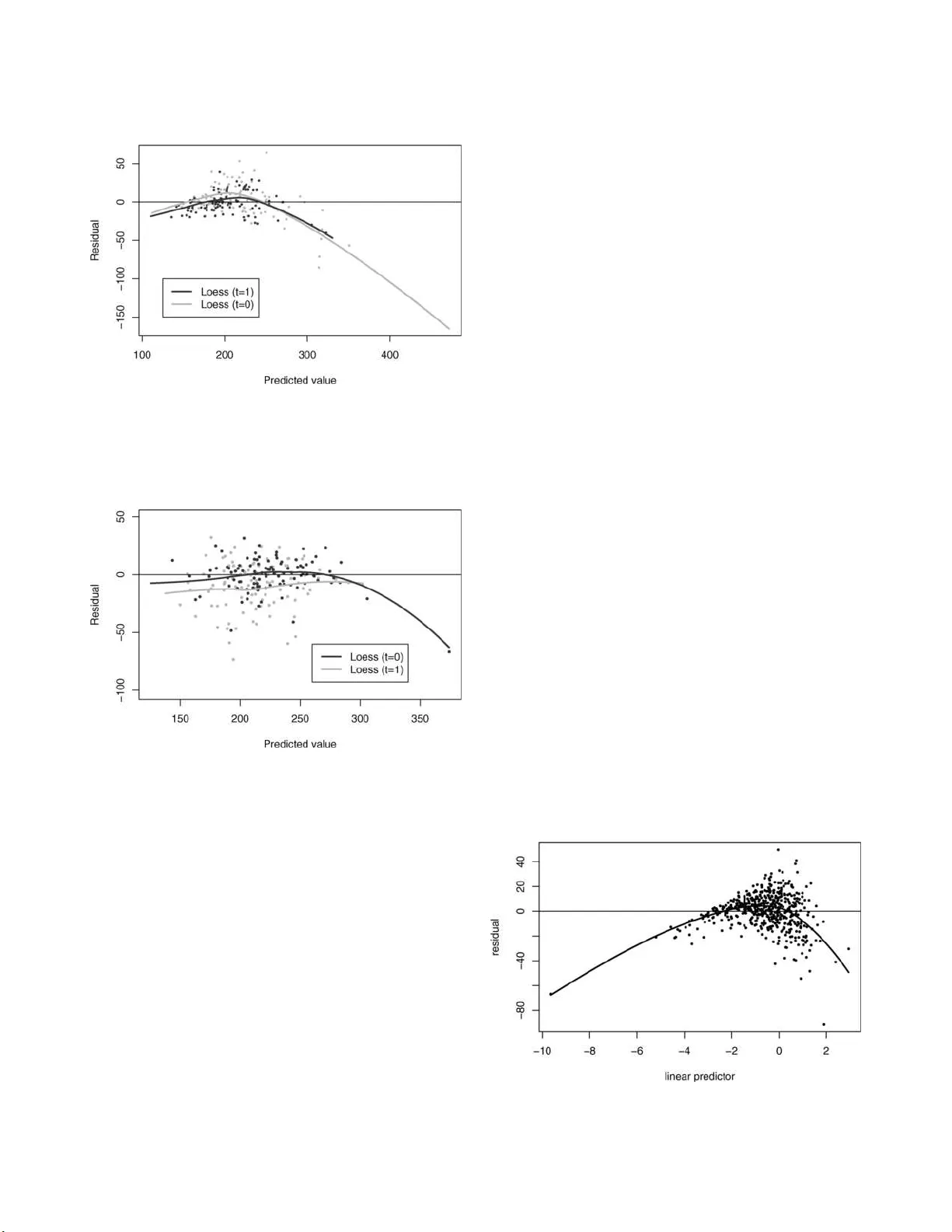
Statistic al Scienc e 2007, V ol. 22, No. 4, 574– 580 DOI: 10.1214 /07-STS227REJ Main article DO I: 10.1214/07-STS227 c  Institute of Mathematical Statisti cs , 2007 Rejoinder: Demystifying Double Robustness: A Compa rison of Alternative Strategies fo r Estimating a P opulation Mean from Incomplete Data Joseph D. Y. Kang and Joseph L. Schafer 1. CLARIFYING OUR POSITION ON D OUBL Y ROBUST ESTIMA TORS W e are grate ful to the editors f or eliciti ng com- men ts from some o f the most prominen t researc hers in this exciting and rapidly deve loping field. After w e drafted our article, a num b er of imp ortan t works on DR est imators app eared, including T an’s ( 2006 ) article on causal inference, the monograph by Tsiatis ( 2006 ) and the recen t articles and technical rep orts cited by Robins, Sued, Lei-Gomez and Rotnitzky . The discussan ts’ insigh tful remarks highlight th ese recen t dev elopments and br ing us up to date. Our pu rp ose in writing this article w as to p ro- vide unfamiliar readers with gentle in tro du ction to DR esti mators without the language of influence functions, using only simple concepts from regres- sion analysis and su rv ey inference. W e w an ted to sho w that DR estimators come in many differen t fla v ors. An d, without minimizing the imp ortance of the literature spa wned by Robins, Rotnitzky and Zhao ( 1994 ), w e w an ted to draw atten tion to some older related m etho ds from mo del-assisted survey sampling whic h arrive at a similar p osition from the opp osite d irection. Joseph D. Y. Kang is R ese ar ch Asso ciate, The Metho dolo gy Center, 204 E. Calder Way, Suite 400, State Col le ge, Pennsylvania 16801, USA e-mail: josephka ng@stat.psu.e du . Joseph L. Schafer is Asso ciate Pr ofessor, The Metho dolo gy Center, The Pennsylvania State University, 204 E. Calder Way, Suite 400, State Col le ge, Pennsylvania 16801 , USA e-mail: jls@stat.psu.e du . This is an e le c tronic r eprint of the origina l a rticle published by the Institute of Mathematica l Statistics in Statistic al Scienc e , 2007, V ol. 22, No. 4, 57 4–58 0 . This reprint differs from the original in pagina tion and t yp ogr aphic detail. Despite the go o d p erformance of ˆ µ OLS in our sim- ulated example, we ha v e n ot and would not argue that it b e used routinely and un critically . The pit- falls of relying solely on outcome regression or y - mo deling hav e b een we ll do cum ented for causal in- ference, where the rates of missin g inf ormation are high and the impact of selection bias can b e dra- matic (e .g., Rubin, 2001 ). Nor d o we wish to cast clouds of sus picion o v er all DR estimators in all cir- cumstances. In many situations, they do work well. On the other h and, w e still b eliev e that pro cedures motiv ated b y parametric y -mo d els, w h en carefully implemen ted, remain a viable option and sh ould not b e categ orically d ismissed. Under ignorabilit y , the pr op ensities π i = P ( t i = 1 | x i ), i = 1 , . . . , n , pla y n o role in likel iho o d-based or Ba yesia n inference ab out µ und er a giv en y -mo del. If w e had absolute faith in one parametric form for P ( y i | x i ), then w e could d iscard all information b e- y ond th e su fficien t statistics for that mo del. But the prop en s ities carry information th at h elps us ev alu- ate the qualit y of the y -mo del, and we ignore this extra information at our p eril, b ecause no mo del is ab o v e criticism. No sensible statisticia n w ould ar- gue that prop ensities should not b e examined. But reasonable p ersons may differ ov er what role the prop en s ities should pla y in form ulating an estima- tor. Those who fa v or a semiparametric approac h d e- vise influence functions that combine inv erse-prop en- sit y weig hts with r egression predictions f or y . Pa ra- metric mo d elers, on the other hand, may well argue that if the prop ensities r ev eal w eaknesses in th e y - mo del, th en that mo d el should b e revised and cor- rected. The latter view has b een exp r essed b y El- liott and Little ( 2000 ) in the cont ext of surv ey esti- mation, where the selection probabilities are kn own, but parallels to uncontrolle d nonresp onse and causal inference are ob vious. 1 2 J. D. Y. KANG A ND J. L. SCHAFER W e b eliev e th at prop ensities are us eful for mo d el diagnosis and estimation, but w e are still not con- vinced that th ey need to en ter an influence func- tion as inv erse-prop ensit y w eigh ts. The strength of w eigh ting is that, if done prop erly , it p rotects an es- timate from b ias regardless of ho w y is d istributed. But this strength can also b e a w eakness, b ecause suc h a high lev el of protection is n ot alw ays war- ran ted. If the prop en sities are u nrelated to th e lin- ear predictors from a goo d y -mo del, then weig hting ma y be sup erfluous. If the prop ensities are p o orly estimated or extreme, then com bin in g w eights with the regression predictions m a y do more harm than go o d. And if the pr op ensities d o rev eal w eaknesses in the y -mo del, inv erse-prop ensit y w eight s are not the only wa y to correct them. 2. RESPONS E TO TS IA TIS AND D A VIDIAN In their ill umin ating discu s sion, Tsiatis and Da- vidian demonstrate that a wide v ariety of estima - tors for µ can b e expressed as th e solution to an estimating equation based on an in fluence function. (One p ossible exception is the class of estimators based on pr op ensity- score matc hing, whic h w e ha ve not discussed.) Influence f unctions present in terest- ing results on semiparametric efficiency , b ut w e find them app ealing for other reasons as wel l. First, they sho w us how to compute a standard error for what- ev er estimator we c ho ose. Second, they generalize nicely to fin ite-p opulation sample surveys with com- plex designs. Regression tec hn iqu es for complex su r- v eys, as implemen ted in soft wa re pac k ages lik e SU- D AAN (S h ah, Barn w ell and Biler, 1997 ), are based on weig hted influ ence functions, s o an y of the es- timators describ ed by Tsiatis an d Da vidian can b e extended to su rve ys. Th ird, if we mo v e on to causal inference, w e must address the thorny issu e of the inestimable partial correlation b et wee n th e p oten- tial ou tcomes. An y estimato r of an a v erage causal effect makes a working assumption ab out this cor- relation (e.g., setting it to zero), b ut a s tand ard error computed from an influ en ce-function sand wic h ma y still p erform well wh en this working correlation is incorrect. Tsiatis and Davidian men tion that our estimator ˆ µ π -c ov , whic h in corp orates prop ensity-rela ted basis functions in to the OLS pr o cedure, is n ot consistent under M I ∪ M II unless the conditional m ean of y i happ en s to b e a linear com b ination of the particular basis fun ctions for π i used in the OR mo d el. This is certainly tru e for the usual asymp totic sequ ence in whic h the num b er of basis fun ctions remains fixed as n → ∞ . But if w e allo w the basis to gro w with the sample size (e.g., as in a smo othing sp line), then it may b ecome DR (Little and An, 2004 ). Giv en a large sample, a go o d data analyst w ill tend to fit a ric her mo d el than with a small sample. If the analyst is allo w ed to bu ild a rich O R model that corrects for the kind of inadequacies sho w n in our Figure 4 , then the OL S pro cedur e based on the corrected OR mo del m a y b e as goo d as an y DR pro cedure. W e like the s uggestion by Tsiatis and Da vidian of u sing a h ybrid estimator that com bines inv ers e- prop en s it y w eigh tin g f or cases with mo derate p rop en- sit y and regression pred ictions for cases w ith small prop en s it y , an idea echoed by v an der Laan and Ru- bin (2006). As an alternativ e to a hard threshold δ at which th e c hange is made, one could opt for a smo other transition by “weig hti ng” eac h part of the influence fu nction more or less d ep end ing on the estimate d p rop ensity . W e also agree with Tsi- atis and Da vidian that estimators in the sp ir it of ˆ µ π -c ov deserv e more consideration ev en though they are not DR o ver M I ∪ M II in the us ual asymptotic sequence. In the sim ulations of our article, w e ex- pressed m i as a piecewise constant fun ction of ˆ π i with discon tin uities at the sample quintiles of ˆ π i . Another v ersion of ˆ µ π -c ov that we ha v e foun d to w ork wel l in m an y situations uses a linear spline in ˆ η i = log( ˆ π i / (1 − ˆ π i )) with kn ots at the q u in tiles. 3. RESPONS E TO T AN T an’s imp ortan t w ork on regression estimators con- nects the theory of influence functions to ideas of surve y regression estimators and the u s e of control v ariates in imp ortance sampling. His remarks and prop ositions are v ery helpful for und erstanding the b ehavio r of IPW, OR an d DR metho ds in realistic settings w h ere all the mo dels are incorrect. W e w ere initially puzzled b y several of T an’s p oint s but, up on f u rther consideration, found them to b e v ery insight ful. He states that it is more construc- tiv e to v iew DR estimators as efficiency-enhanced v ersions of IPW than as bias-co rrected v ers ions of OR. W e find b oth views helpful for un derstanding the n ature and pr op erties of DR metho d s. But, as he explains, there are theoretical r easons to exp ect that his carefully crafted DR estimators ma y lead to greater improv emen t ov er IPW than ov er a go o d O R mo del, b ecause IPW is conserv ativ e wh er eas O R is aggressiv e. REJOINDER 3 W e are still unsu re w h y T an states th at IPW ex- trap olates explicitly whereas O R extrap olates im- plicitly . T o us, fitting an O R mo del to resp ond en ts and us in g that mo del to predict for nonresp onden ts is a v ery obvio us kin d of extrap olation, esp ecially if the lev erage v alues for some nonresp onden ts are large rela tiv e to those of the resp ondent s. But his p oints ab out extrap olation are well tak en. All of our metho ds extrap olate . The assumption of ignorabil- it y is itself an extrap olation. He also p oints out that estimating an a ve rage causal effect is more su btle than simp ly estimating the m ean of eac h p oten tial outcome and taking th e d ifference. This distinction is imp ortan t in a semip arametric approac h. A semiparametric metho d that is optimal for estimating t wo means ma y not b e optimal for estimating the m ean d ifferen ce. Similarly , a metho d that is optimal for estimating a p opulation a verage causal effect may not b e optimal for estimating the a verage effect among the treated, or for estimating differences in a ve rage causal effects b etw een subp op- ulations. As parametric assumptions ab out th e O R mo del are discard ed, it b ecomes imp ortan t to tailor the estimation pro cedu re to the estimand, which his regression estimato rs apparently do. In T an’s simulatio ns, his alternativ e mo del in which the analyst sees X 4 = ( Z 3 + Z 4 + 20) 2 present s an in- teresting situation where O L S predicts the y i ’s for the resp onden ts almost p erfectly ( R 2 ≈ 0 . 99), bu t the extrap olate d linear predictions for the nonr e- sp ond en ts are biased b ecause the unseen tru e v alues of y i turn sh arply a wa y from those predictions in th e region of lo w p r op ensity . This is a p er f ect illustration of ho w the u ncritical u se of ˆ µ OLS can lead us astra y . But in this example, prop ensit y-b ased diagnostics rev eal ob vious d eficiencies in the linear mo d el. T ak- ing the initial sample of n = 200 observ ations from our article, w e fit the linear mo del to the resp on - den ts and a logistic prop ensit y mo del to all cases giv en X 1 , X 2 , X 3 , and T an’s alternativ e v ers ion of X 4 . A plot of the observed r esiduals from the y - mo del v ersus the estimated logit-prop ensities from the π -mo del is sh o wn in Figure 1 . The lo ess cur ve clearly sho w s that the OLS predictions are biased in the r egion of high prop ensit y (where it do es not really matter) and in the regio n of lo w prop ensit y (where it matters v ery muc h ). If w e accoun t for this trend by in tro du cing the squared linear predictor from th e logi t mo d el ˆ η 2 i = ( x T i ˆ α ) 2 as one more co v ari- ate in th e y -mo del, th e p erf ormance of ˆ µ OLS greatly impro ve s. Even b etter p erf ormance is obtained with splines, w hic h tend to pr edict b etter than ord inary p olynomials ov er the whole range of ˆ η i ’s. W e created a linear spline basis for ˆ η i with four kn ots lo cated at the sample quin tiles of ˆ η i . That is, w e added the four co v ariates ( ˆ η i − k 1 ) + , ( ˆ η i − k 2 ) + , (1) ( ˆ η i − k 3 ) + , ( ˆ η i − k 4 ) + to the y mo del, where ( z ) + = max(0 , z ) and k 1 , k 2 , k 3 , k 4 are the knots. Ov er 1000 samples, w e found that this new version of ˆ µ OLS (whic h, in our article, w e w ould hav e called ˆ µ π -c ov ) p erformed as w ell as any of T an’s estimators in the scenario wh ere b oth mo d- els were incorrect. With n = 200, we obtained bias = 0 . 16, % bias = 5 . 70, RMSE = 2 . 78 and MAE = 1 . 78. With n = 1000, w e obtained b ias = 0 . 30, % bias = 24 . 6, RMSE = 1 . 27 and MAE = 0 . 88. The p erfor- mance of T an’s regression estimators in these sim- ulations is impressive. Th e p erformance of ˆ µ OLS is equally impr essiv e if we allo w the an alyst to m ake a simple correction to adj ust for the y -mo del’s ob vious lac k of fit. 4. RESPONSE T O RIDGEW A Y AND MCCAFFREY Ridgew a y and McCaffrey correctl y observ e that, for estimating prop ensit y scores, there are many goo d alternativ es to logistic regression. I n addition to their w ork on the generalized b o osted mo d el (GBM), some ha v e b een estimating prop en sities using classifica- tion trees (Luellen, Sh adish and Clark, 2005 ) and neural n et w orks (King and Zeng, 2002 ). Fig. 1. Sc atterplot of r aw r esiduals f r om line ar y -mo del fit to r esp ondents i n T an ’ s alternative mo del, versus the line ar pr e- dictors fr om a l o gistic π -mo del, with l o c al p olynomial (lo ess) fit. 4 J. D. Y. KANG A ND J. L. SCHAFER A ric h prop ens it y mo del should impro ve the p er- formance of the we ight ed estimator. Th e adv ant age of pro cedur es lik e classification trees and GBM is that they allo w us to searc h thr ou gh a large space of π -mo dels, accoun ting for the effects of man y co v ari- ates and their in teractions, thereby redu cing bias in the resulting estimator regardless of ho w y i is distributed. These pro cedures m a y also reduce v ari- ance, b ecause, as explained by T an, in a sequence of increasingly ric h pr op ensity mo dels, the asymp- totic v ariance of an augmen ted IPW estimator de- creases to the semiparametric b ound. In principle, one could apply sim ilar pro cedu r es lik e regression trees to create a rich y -mo del. But, as Ridgew a y and McCaffrey p oin t out, this raises the p ossibilit y of data sn o oping. As we searc h through larger and more complicated sp aces to fi nd the b est y -mo del, it b ecomes incr easingly difficult to compute honest standard errors . Ridgew a y and McCaffrey’s simulatio ns with the extra in teraction term again rev eal the dangers of uncritically r elying on ˆ µ OLS . This in teraction in- creases the degree to w hic h the additiv e and lin ear y -mod el is miss p ecified, so in th is scenario we would exp ect the p erformance of ˆ µ OLS to worsen. Th e fin al columns of their T ables 1 and 2 sho w that, when this in teraction is p resen t, prop ens it y -b ased and DR es- timators str on gly outp er f orm ˆ µ OLS . Using the wrong co v ariates in the prop ensit y mo del do es little harm to the flexible GBM pro cedu r e. But one could ar- gue that these comparisons b et ween GBM and ˆ µ OLS are u nfair in the follo wing sense: They resem ble a situation where the analyst is a llo w ed to fit a ric h and flexible π -mo del bu t is giv en no leewa y to im- pro v e the y -mo del. W e examined many samples of n = 200 from this new p opulation and foun d X 1 X 2 to b e a strong and h ighly significant p redictor of y in ev ery sample. If w e add this one in teraction to the y -mod el, th e b ias in ˆ µ OLS nearly v anishes, and its RMS E b ecomes comparable to th at of the b est DR estimators that Ridgew ay and McCaffrey tried. Other in teractions are often signifi can t as we ll. W e ha v e not examined the p erformance of ˆ µ OLS when these other interac tions are in cluded; doing so w ould b e an inte resting exercise. Our p oin t here is not to argue for the su p eriorit y of ˆ µ OLS o ver the DR pro cedures. Either can w ork w ell if applied carefully with appropr iate safeguards. And either can b e made to fail if we , through the design of a simulation, imp ose artificial restrictions that force th e analyst to ignore clear evidence in the observ ed data that the pro cedure is fla wed. 5. RESPONSE T O ROBINS, SUED, LEI-GOMEZ AND ROTNITZKY The commen ts b y Robins et al. con tain man y u se- ful observ ations and helpful references. Their sim u- lations that rev erse th e roles of t i and 1 − t i are instructiv e. Ho wev er, in the pr o cess of arguin g th at w e misundersto o d the message of Bang and Robins ( 2005 ), they h a v e apparen tly misunders to o d ours. Their insinuations of cherry-pic kin g m igh t b e under- standable if we h ad b een arguin g for the sup eriorit y of ˆ µ OLS , but that is n ot what we ha v e done. Quite honestly , w e b egan this inv estigation fully exp ecting to demonstrate the b enefits of dual mo deling when neither mo del is exactly true. When Bang and Rob in s ( 2005 ) r ecommended cer- tain DR pro cedures for routine use, they did so with- out qualifications or cautionary statemen ts. No w they quote a p assage from another article pu blished five y ears earlier, which Bang and Robin s ( 2005 ) d id not cite, to demonstrate th at this w as not what they had in mind. Readers cannot react to what they h a v e in min d , but only to what they write. Dr. Robins and his colleagues are eminent researc h ers, and their statemen ts carry consid erable w eigh t. Th e fact that they knew that these estimators sometimes misb e- ha v e but failed to ac knowle dge it mak es their b lan- k et recommendations in 2005 ev en more troubling. F or the r ecord, w e will clarify ho w we ca me up with our sim ulated example. As men tioned in our Section 4 , w e were trying to lo osely mim ic a quasi- exp eriment to assess the a verag e causal effect of di- eting on b o dy-mass index among adolescen t girls. W e decided b eforehand that y i should b e p redicted from the observ ed x i with R 2 ≈ 0 . 80, as in the ac- tual d ata. W e decided that the distributions of th e estimated prop ensity scores s h ould resem b le those in our Figure 3(e), as in the actual data. W e decided that th e lin ear p redictors fr om the y -mo del and π - mo del should h av e a correlation of at least 0 . 5, as in the actual data, s o that ¯ y 1 = P i t i y i / P i t i w ould b e a strongly biased as an estimator of µ . W e d ecided that the co v ariates in x i should not b e normally d is- tributed, bu t they should n ot b e so hea vily sk ew ed that a data analyst w ould n eed to transf orm them to reduce the lev erage of a few large v alues. W e d ecided that x i m ust b e a one-to-one transformation of the unseen tru e co v ariates z i o ver the effectiv e s upp ort of the z i (without this condition, n onresp onse w ould not b e ignorable give n x i ). Finally , we decided that the linear r egression of y i and th e logistic r egres- sion of t i on x i w ould b e missp ecified to ab out the REJOINDER 5 same exten t, in the sense that the correlati ons b e- t w een the linear predictors f rom eac h mo del and the corresp ondin g true linear predictors would b e ab out 0.9. After considerable trial and er r or, we came up with one example that met all of these criteria. As w e ran our sim ulations, w e w ere truly surprised to see ˆ µ OLS p erform as w ell as it d id, consistently b eat- ing all comp etitors. W e exp ected that at least some of the DR estimators would improv e up on ˆ µ OLS , bu t none did. In fact, w e were tempted to lo ok for a dif- feren t example that wo uld demonstrate some of the b enefits of DR, but we d ecided against it precisely b ecause we wan ted to avoid cherry-pic king. As Robin s et al. deconstruct our sim ulated exam- ple, they su ggest that our missp ecified linear mo del E ( y i ) = x T i β is so close to b eing true that ˆ µ OLS is virtually guaran teed to outp erform all comp etitors. If that w ere so, then w h y d id th e DR estimators ˆ β WLS and ˆ µ BC-OLS not p erform as well, as th ose es- timators w ere giv en the same opp ortun it y to take adv an tage of this nearly correct y -mod el? And, if that were so, why would ˆ µ OLS p erform so p o orly in their simulati ons when the r oles of t i and 1 − t i w ere rev ersed? The firs t plot in Figure 1 by Robins et al. rev eals that (a) th e mo del for y i giv en the v ector of true co v ariates z i is a linear with v ery high R 2 and (b) the nonresp onse is ignorable, so that P ( y i | z i , t i = 1) and P ( y i | z i , t i = 0) are the same. Th is plot im- plies that conditions where the analyst is allo w ed to see the z i ’s are unrealistic, b ecause kno wing z i is essen tially equiv alen t to knowing y i . Bu t this plot sa ys n othing ab out the p erformance of ˆ µ OLS or any other estimator when z i is hidden and the analyst sees only x i , w h ic h is the on ly scenario th at we hav e claimed is realistic. [In fact, the first simulat ed ex- ample publish ed b y Bang and Robins ( 2005 ) yields a similar picture, b ecause their true d ata-generati ng mec h anism is also linear and their R 2 is 0.94.] The conditional v ariance V ( y i | z i ) w as one of man y pa- rameters that w e had to adjust to create an example that satisfied all of the criteria that we hav e men - tioned. W e tried to s et V ( y i | z i ) to larger v alues, but doing so decreased the signal-t o-noise ratio in the observ ed data to the p oint w here we no longer sa w meaningful b iases in any estimators wh en n = 200. With their Figure 2 , Robin s et al. p u rp ort to show that our m iss p ecified linear r egression mod el fits so w ell that the predicted v alues x T i ˆ β are essentiall y unbiase d pr edictions of th e missing y i ’s, which guar- an tees excellen t p erf ormance for ˆ µ OLS . They state, “W e can see that the p redicted v alues of the nonre- sp ond en ts are reasonably cent ered aroun d the straigh t line ev en for th ose p oin ts with pred icted v alues far from the predicted v alues of the r esp ondents.” On the con trary , ou r linear m o del E ( y i ) = x T i β d o es n ot giv e unbiased pr edictions for nonresp onden ts or re- sp ond en ts, esp ecially not in the region of extrap ola- tion. T o illustrate, w e to ok one sim ulated samp le of n = 1000 observ ations, regressed y i on x i among the resp ond en ts, and computed the r egression predic- tions x T i ˆ β and residu als y i − x T i ˆ β for b oth groups. A p lot of the residuals versus the regression pr e- dictions is d isp la y ed in Figure 2 , along with lo cal p olynomial (lo ess) tren d s. Resp ondents are sho wn in blac k, and nonresp onden ts are sho wn in gra y . (F or visual clarit y , only 20% of the p oin ts are dis- pla y ed, but the lo ess trends are estimated from the full sample.) F or eac h group, the least-squares r e- gression mo del strongly u nderpr edicts n ear the cen- ter and o v erpredicts at the extremes. Th e reason wh y ˆ µ OLS p erforms w ell in this example is n ot that the linear mo d el is appr o ximately tru e, but that the p ositive and ne gative r esiduals in the nonr esp ondent gr oup app r oximately c anc el out. The a v erage v alue of y i − x T i ˆ β f or resp onden ts is exactly zero (a conse- quence of OLS ), and the a v erage v alue of y i − x T i ˆ β for nonresp onden ts is close to zero. Ove r 1000 sim- ulated samples, the a v erage of y i − x T i ˆ β among non- resp ond en ts was 1.68. Multiplying this by − 0 . 5 (b e- cause the a v erage nonresp onse rate is 50%) gives − 0 . 84, th e estimated bias for ˆ µ OLS rep orted in our T able 3. Figure 2 also rev eals why ˆ µ OLS w as n ot b eaten in this example by an y of the d ual-mo deling m eth- o ds. The d ifferences b et wee n the tw o lo ess cu rv es in Figure 2 are not large, sho wing that the OL S predic- tions hav e similar patterns of bias for r esp ondents and nonresp ondent s. When the predictions from a y -mod el are b iased, and the biases are similar when t i = 1 and t i = 0, they are not easily corrected by an estimated pr op ensity m o del. If we reverse the roles of t 1 and 1 − t i , as Robins et al. ha v e done, the situation dr amatically c hanges. T aking the same sample of n = 1000, we r egressed y i on x i when t i = 0 and pr edicted the resp onses f or b oth groups. Residuals v ersus predicted v alues f rom this rev erse fit are sh o wn in Figur e 3 . (Once again, for visual clarity , only 20% of the samp led p oint s are shown, but the lo ess trends are estimated from 6 J. D. Y. KANG A ND J. L. SCHAFER Fig. 2. R esiduals versus pr e dicte d values f or r esp ondents ( t i = 1 ) (black dots) and nonr esp ondents ( t i = 0 ) (gr ay dots) fr om one sample of n = 1000 fr om our original simulation, with lo c al p olynomial (lo ess) tr ends f or e ach gr oup. F or visual clarity, only 20% of the sample d p oints ar e shown. Fig. 3. Plot analo gous to Figur e 2 , with the r oles of t i and 1 − t i r everse d. Cases with t i = 0 and t i = 1 ar e denote d by black and gr ay dots, r esp e ctively, wi th lo c al p olynomial (lo ess) tr ends shown f or e ach gr oup. F or visual clarity, only 20% of the sample d p oints ar e shown. the fu ll samp le.) F or the t i = 0 group, the linear mo del underp redicts at the cen ter and o v erpredicts at the extremes, and the a verage v alue y i = x T i ˆ β is zero. But for the t i = 1 group, the linear mo d el con- sisten tly o v erpredicts across the entire range, in tro- ducing a strong up wa rd bias into ˆ µ OLS . This alternativ e sim ulation by Robins et al. is a classic example where patterns of bias in a linear y -mod el cause ˆ µ OLS to p erform p oorly . Bu t b ecause the patterns are dr amaticall y different when t i = 0 and t i = 1, it is also a classic example where the fail- ure can b e readily diagnosed and corrected by fi tting a π -mo del. A plot of the residuals y i − x T i ˆ β for the t i = 0 group v ersu s the linear predictors from a lo- gistic p rop ensity mo del is sh o wn in Figure 4 . The plot, whic h is based only on ( x i , t i , (1 − t i ) y i ), shows a strong tendency for the linear y -mod el to o v erpre- dict w hen P ( t i = 1) is lo w or high. T o correct this bias, we created a spline b asis as in expr ession ( 1 ), with knots at the sample qu in tiles, and included the four extra term s as predictors in the linear y -mo d el. The p erformance of ˆ µ OLS (whic h w e w ould no w call ˆ µ π -c ov ) impro v ed d ramatically , and the new estima- tor w ork ed b etter th an any of the d ual-mo deling metho ds rep orted b y Robins et al. Th e p erformance statistics in the b oth-mod els-wrong scenario w ere Bias = 2 . 21, V ar. = 12 . 61 and MSE = 17 . 46 wh en n = 200, and Bias = 2 . 40, V ar. = 1 . 88, and MSE = 7 . 66 when n = 1000, whic h compare f a v orably to the results s h o wn b y Robin s et al. in their T able 2. 6. CONCLUDING REMARKS As statisticians d evise n ew er and fancier metho ds, w e hop e to find one that is fo olpro of, yielding go o d results n o matter when and ho w it is app lied. But the searc h for a fo olpr o of metho d is qu ixotic and futile. Some pr o cedures are, on b alance, b etter than others, bu t eac h one requires man y su b jectiv e in - puts, and none should b e applied routinely or u ncrit- ically . As we dev elop b etter estimat ors, we should also strive to giv e p oten tial users a h ealth y d ose of in tuition ab out how the pro cedu res work, their lim- itations, soun d recommendations ab out their use, and diagnostics that can help users decide when a pro cedur e is tru st w orthy and when it is not. In conclusion, we b elieve that prop ensity mo deling is p rudent and eve n necessary wh en rates of missin g information are high. Bu t w e are still not convinced Fig. 4. Sc atterplot of r esiduals fr om a line ar y -mo del fit to t i = 0 c ases, versus line ar pr e dictors f r om a lo gistic π -mo del, with lo c al p olynomial (lo ess) fit in one sample of n = 1000 fr om the alternative simulation study by R obi ns et al. REJOINDER 7 that estimated inv erse prop ensities m ust alw a ys b e used as w eigh ts. A CKNO WLEDGMENT This researc h w as supp orted b y National I nstitute on Dru g Abuse Gran t P50-D A10075. REFERENCES Bang, H . and Rob ins, J. M. ( 2005). Doub ly robust estima- tion in missing data and causal inference mo dels. Biomet- rics 61 962–972. MR2216189 Elliott, M. R. and Little, R. J. A. (2000). Mo del-based alternativ es to trimming su rvey weigh t s. J. Official Statis- tics 16 191–209. King, G. and Zen g, L. (2002). I mproving forecasts of state failure. World Politics 53 623–658. Little, R. J. A. and An, H. (2004). Robust likeli ho o d-based analysis of multiv ariate data with missing va lues. Statist. Sinic a 14 949–968. MR2089342 Luellen, J. K., Sh adish, W. R. and Clark, M. H. ( 2005). Propensity scores: An introduction and exp erimental test. Evaluation R eview 29 530–558. Ro bins, J. M., Rotnitzky, A. and Zha o, L. P. (1994). Estimation of regression coefficients when some regressors are not alw a ys observed. J. A mer. Statist. Asso c. 89 846– 866. MR1294730 Rubin, D. B. (2001). Using p rop en sit y scores t o help design observ ational studies: Applications to the tobacco litiga- tion. He alth Servic es and Outc omes R ese ar ch Metho dolo gy 2 169–188. Shah, B. V., Barnwell, B. G. and Bile r, G. S. (1997). SUDAAN User’s Manual, R ele ase 7.5 . Researc h T riangle P ark, Research T riangle In stitu te, NC. T an, Z. (2006). A distributional approac h for causal inference using propensity scores. J. Amer . Statist. Asso c. 101 1619– 1637. MR2279484 Tsia tis, A . A. (2006). Semip ar ametric The ory and Missing Data . Springer, New Y ork. MR2233926