Boosting Algorithms: Regularization, Prediction and Model Fitting

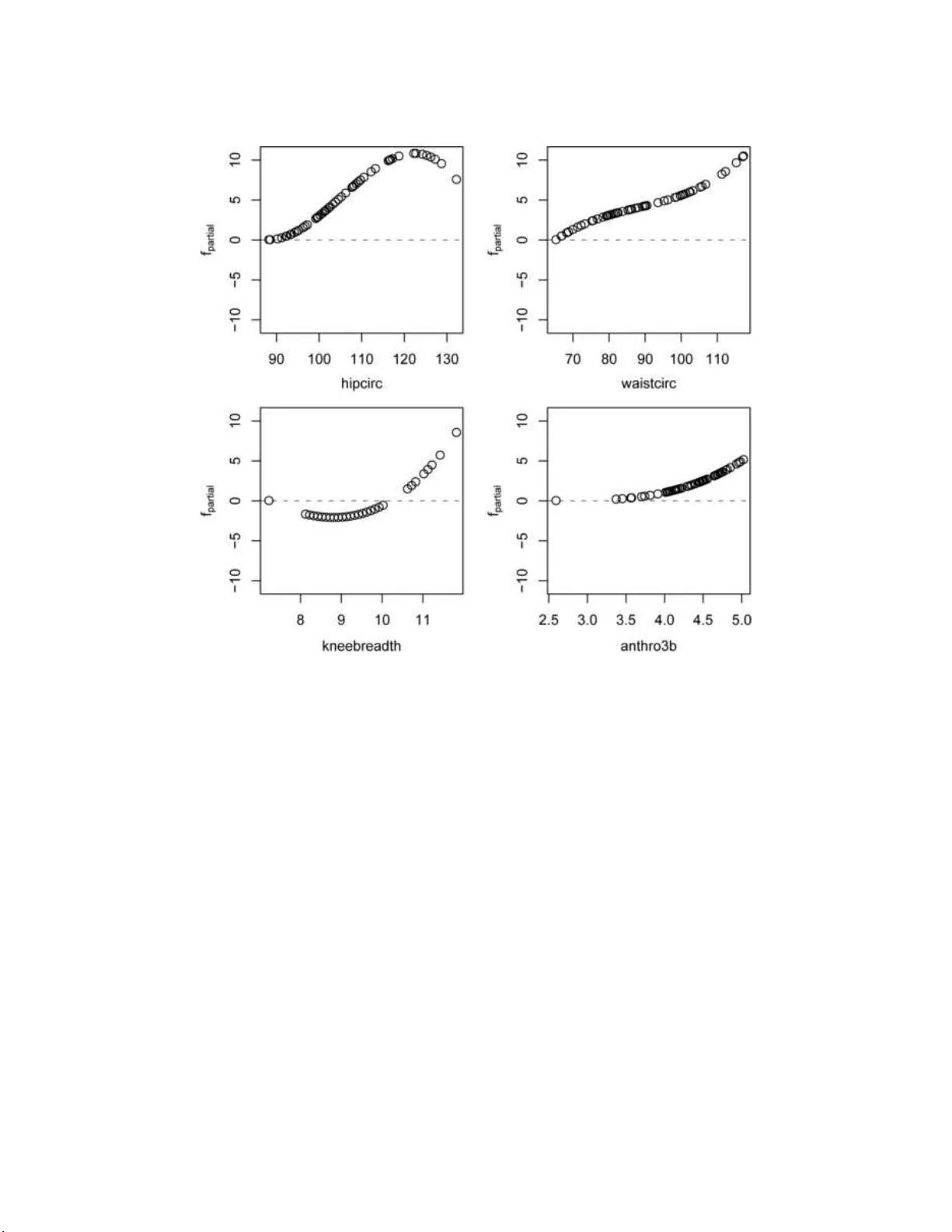
Statistic al Scienc e 2007, V ol. 22 , N o. 4, 477– 505 DOI: 10.1214 /07-STS242 c  Institute of Mathematical Statistics , 2007 Bo osting Algo rit hms: Regula rizat ion, Prediction and Mo del Fitting P eter B¨ uhlmann a nd T o rsten Hotho rn Abstr act. W e presen t a statist ical p ersp ectiv e o n b o osti ng. Sp ecial emphasis is giv en to estimating p oten tially complex parametric or non- parametric mo dels, including generalized linear and additiv e mo dels as w ell as regression mod els for surviv al analysis. Concepts of degrees of freedom and corresp onding Ak a ike or Ba y esian information crite- ria, particularly u seful for r egularizat ion and v ariable selectio n in high- dimensional co v ariate spaces, are discussed as well. The practical asp ects of b o osting pro cedur es for ﬁtting statistical mo dels are illustrated by means of the dedicated op en-source soft ware pac k age mb o ost . This pac k age imp lements functions whic h can b e used for mo del ﬁtting, prediction and v ariable selection. It is ﬂexible, al- lo w in g for the implemen tation of new b o osting algo rithms optimizing user-sp eciﬁed loss f u nctions. Key wor ds and phr ases: Generalized linear mo d els, generalized ad- ditiv e mo dels, gradien t bo ost ing, surviv al analysis, v ariable selection, soft w are. 1. INTRODUCTION F reund and Sc hapire’s AdaBoost algorithm for clas- siﬁcation (author?) [ 29 , 30 , 31 ] has attrac ted m uch atten tion in the machine learning comm u nit y (cf. [ 76 ], and the references therein) as w ell as in related areas in statistic s (author?) [ 15 , 16 , 33 ]. V arious ver- sions of the AdaB o ost algo rithm ha v e pro ven to b e v ery comp etitiv e in terms of prediction accuracy in a Peter B ¨ uhlmann is Pr ofessor, Seminar f¨ ur Statistik, ETH Z ¨ urich, CH-8092 Z¨ u rich, Switzerland e-mail: buhlmann@stat.math.ethz.ch . T orsten H othorn is Pr ofessor, Institut f ¨ ur S t atistik, Ludwig-Maximili ans-Universit¨ at M¨ unchen, Ludwigstr aße 33, D- 80539 M¨ un chen, Germany e-mail: T orsten.Hothorn@R-pr oje ct.or g . T orsten Hothorn wr ote this p ap er while he was a le ctur er at the Universit¨ at Erlangen-N¨ urnb er g. 1 Discussed in 10.121 4/07-STS242A and 10.121 4/07-STS242B ; rejoinder at 10.1214/07 -STS242REJ . This is a n electro nic r eprint o f the o riginal a rticle published b y the Ins titute of Mathematica l Statistics in Statistic al Scienc e , 200 7, V ol. 22, No. 4, 477 –505 . This reprint diﬀers fro m the original in pag ination and t yp ogr aphic detail. v ariet y of applications. Bo osting metho ds h a v e b ee n originally prop osed as ens em ble metho ds (see Sec- tion 1.1 ), whic h rely on the principle of generating m ultiple predictions and ma jorit y voti ng (a v erag- ing) among the individu al classiﬁers. Later, Breiman (author?) [ 15 , 16 ] made a path- breaking observ ation that the AdaBo ost algorithm can b e view ed as a gradient descen t algorithm in function sp ace, inspired by n umerical optimizat ion and sta tistical estimation. Moreo v er, F r iedman, Hastie and Tibshirani (author?) [ 33 ] laid out fur ther i m- p ortan t foundations w hic h link ed Ada-Boost and other b oosting algo rithms to the framew ork of sta - tistical estimat ion and additiv e basis expansion. In their terminology , b o osti ng is repr esen ted as “stage- wise, add itiv e mo deling”: the w ord “additiv e” do es not imply a mo del ﬁ t wh ic h is additive in the co- v ariates (see our S ection 4 ), b ut r efers to the fact that b o osting is an additiv e (in fact, a linear) com b i- nation of “simple” (function) estimat ors. Also Ma- son et al. (author?) [ 62 ] and R¨ atsc h, On o da and M ¨ uller (author?) [ 70 ] deve lop ed related ideas whic h w ere mainly ac kno wledged in the mac hine learning comm unit y . In Hastie, Tibsh irani and F r iedman (au- thor?) [ 42 ], add itional views on b o osting are giv en; 1 2 P . B ¨ UHLMANN AN D T. HOTHOR N in particular, t he authors ﬁrst p oin ted out the re- lation b et wee n b o osting and ℓ 1 -p enalized esti ma- tion. The insights of F riedman, Hastie and Tibshi- rani (author?) [ 33 ] op ened new p ersp ecti ve s, namely to use bo osting m etho ds in many other conte xts than classiﬁcation. W e m en tion h ere b oosting meth- o ds for r egression (including generalized regression) [ 22 , 32 , 71 ], for densit y estimat ion [ 73 ], for surviv al analysis [ 45 , 71 ] or for m ultiv ariate analysis [ 33 , 59 ]. In quite a few of th ese pr op osals, b oosting is not only a blac k-b o x prediction to ol b ut also an estimation metho d for mo dels with a sp eciﬁc stru cture such as linearit y or add itivit y [ 18 , 22 , 45 ]. Boosting can then b e seen as an in teresting regularizatio n sc heme for estimating a mo del. This statistica l p ersp ectiv e will driv e the fo cus of our exp osition of b oosting. W e present here some co herent expla nations and illustrations of concepts ab out b oosting, s ome d eriv a- tions wh ic h are no ve l, and we aim to increase the understanding of some metho d s and some selected kno wn results. Besides giving an o v erview on th eo- retical concepts of b o osting as an algorithm for ﬁt- ting statisti cal models, w e lo ok at the metho dology from a practical p oin t of view as w ell. Th e d edicated add-on pac k age m b oost (“mo del-based b o osting,” [ 43 ]) to the R system f or statist ical computing [ 69 ] implemen ts compu tational to ols whic h enable the data analyst to compu te on the theoretical concepts explained in this pap er as closely as possible. T h e illustrations p resen ted t hr oughout the pap er f o cus on thr ee r egression problems with con tin uous, b i- nary an d censored resp onse v ariables, some of them ha ving a large n umb er of co v ariates. F or ea c h ex- ample, w e only present the most imp orta nt steps of the analysis. The co mplete analysis is con tained in a vignette as part of the mbo ost pac k age (see Ap- p endix A.1 ) so that ev ery result s h o wn in this pap er is r epro ducible. Unless stated diﬀerentl y , we assu me that the d ata are realiza tions o f r and om v ariables ( X 1 , Y 1 ) , . . . , ( X n , Y n ) from a stationary p ro cess with p -dimens ional predic- tor v ariables X i and one-dimensional resp onse v ari- ables Y i ; for the case of multi v ariate resp onses, some references are g ive n in Section 9.1 . In parti cular, the setting ab ov e includes indep end en t, identic ally distributed (i.i.d.) observ ations. The generaliza tion to stationary pr o cesses is f airly s traigh tforward: the metho ds and algorithms are the same as in the i.i.d. framew ork, but the mathematical theory requires more elab orate tec hn iques. Essential ly , one needs to ensure that some (uniform) laws of large num b ers still h old, for example, assuming stationary , mixing sequences; some rigorous r esults are give n in [ 57 ] and [ 59 ]. 1.1 Ensemble Schemes : Multiple Prediction and Aggregation Ensem ble sc h emes construct multiple fun ction es- timates or predictions from reweig hted data and use a linear (or sometimes con ve x) c ombinati on thereo f for pro ducing the ﬁnal, aggregated estimator or pre- diction. First, w e sp ecify a b ase pr o c e dur e which constructs a function est imate ˆ g ( · ) with v alues in R , based on some data ( X 1 , Y 1 ) , . . . , ( X n , Y n ): ( X 1 , Y 1 ) , . . . , ( X n , Y n ) base procedure − → ˆ g ( · ) . F or example, a ve ry p opular base p ro cedure is a re- gression tree. Then, generating an ensem ble from the base pro- cedures, that is, an ensemble of function estimates or p redictions, w orks generally as follo ws: rew eigh ted data 1 base procedure − → ˆ g [1] ( · ) rew eigh ted data 2 base procedure − → ˆ g [2] ( · ) · · · · · · · · · · · · rew eigh ted data M base procedure − → ˆ g [ M ] ( · ) aggrega tion: ˆ f A ( · ) = M P m =1 α m ˆ g [ m ] ( · ) . What is termed here as “reweig hted data” means that we assign individual data w eigh ts to eac h of the n sample p oin ts. W e ha ve also implicitly as- sumed that the base p ro cedure allo ws to do some w eigh ted ﬁtting, that is, estimation is based on a w eigh ted sample. Throughout the p ap er (exce pt in Section 1.2 ), w e assume that a base pro cedur e esti- mate ˆ g ( · ) is real-v alued (i.e., a r egression p r o cedure), making it more adequate for the “statistica l p ersp ec- tiv e” on b o osting, in particular for the generic FGD algorithm in Section 2.1 . The ab ov e description o f an ensemble sc h eme is to o general to b e of an y direct use. The sp ec iﬁcation of the data rew eigh ting mechanism as w ell as the form of the linear com bination co eﬃcien ts { α m } M m =1 are cru cial, and v arious c hoices c haracterize d iﬀer- en t ensemble scheme s. Most b oosting metho ds are sp ecial kinds of se quential ensem ble schemes, w here the data wei ghts in iteration m dep end o n the results BOOSTING ALGORITHMS A ND MODEL FITTING 3 from the previous iteration m − 1 only ( memoryl ess with resp ect to iterations m − 2 , m − 3 , . . . ). Exam- ples of other ensem ble sc hemes include bagging [ 14 ] or r andom forests [ 1 , 17 ]. 1.2 AdaBo ost The AdaBo ost algo rithm for binary c lassiﬁcation [ 31 ] is the most w ell-kno wn b oosting algorithm. The base pro cedure is a classiﬁer with v alues in { 0 , 1 } (sligh tly diﬀerent from a real-v alued function esti- mator as assumed abov e), for example, a classiﬁca- tion tree. AdaBoost alg orithm 1. In itialize some wei ght s for individual samp le p oint s: w [0] i = 1 /n for i = 1 , . . . , n . Set m = 0. 2. In crease m by 1. Fit the base p ro cedure to the w eigh ted data, that is, do a weigh ted ﬁtting u sing the we igh ts w [ m − 1] i , yielding the classiﬁer ˆ g [ m ] ( · ). 3. Comp ute the weig hte d in-sample misclassiﬁca- tion rate err [ m ] = n X i =1 w [ m − 1] i I ( Y i 6 = ˆ g [ m ] ( X i )) . n X i =1 w [ m − 1] i , α [ m ] = log  1 − err [ m ] err [ m ]  , and up date the weig hts ˜ w i = w [ m − 1] i exp( α [ m ] I ( Y i 6 = ˆ g [ m ] ( X i ))) , w [ m ] i = ˜ w i / n X j =1 ˜ w j . 4. Iterate steps 2 and 3 until m = m stop and build the aggregated classiﬁer by we ight ed ma jorit y v ot- ing: ˆ f AdaBoost ( x ) = arg max y ∈{ 0 , 1 } m stop X m =1 α [ m ] I ( ˆ g [ m ] ( x ) = y ) . By using the termin ology m stop (instead of M as in the general description of en s emble schemes), we emphasize here and later that the iteratio n pro cess should b e stopp ed to av oid o verﬁtting. It is a tuning parameter of AdaBo ost wh ic h ma y b e selected u sing some cross-v alidatio n sc heme. 1.3 Slo w Overﬁtting Behavior It had b een debated un til ab out the ye ar 2000 whether the Ad aBo ost algorithm is immune to ov er- ﬁtting when r unning more iterations, that is, stop- ping w ould n ot b e necessa ry . It is clear n o wada ys that Ada-Bo ost and also other bo osti ng algorithms are ov erﬁtting eve ntual ly , and early stopping [using a v alue of m stop b efore con verge nce of the sur rogate loss function, giv en in ( 3.3 ), tak es place] is necessary [ 7 , 51 , 64 ]. W e emphasize that this is not in co n- tradiction to the exp erimen tal results by (a uthor?) [ 15 ] where the test set misclassiﬁcation error still decreases after the training misclassiﬁcation error is zero [b ecause the training error of the su rrogate loss function in ( 3.3 ) is not zero before numerical con- v ergence]. Nev erth eless, the AdaBo ost algorithm is quite r e- sistan t to o ve rﬁ tting (slo w ov erﬁtting b eha vior) when increasing the n u mb er of iterations m stop . This h as b een obs erved empirically , although some cases w ith clear o verﬁtti ng do occur for some datasets [ 64 ]. A stream of w ork has b een dev oted to d evelo p V C-t yp e b ound s for the generali zation (out-of-sample) error to explain why b o osting is o v erﬁtting ve ry slo w ly only . Schapire et al. (author?) [ 77 ] pro ved a remark- able b ound for the generalizati on misclassiﬁcation error for classiﬁers in the con v ex hull of a base pro ce- dure. This b ound for the misclassiﬁcati on error h as b een improv ed by Koltc hin skii and Panc henko (au- thor?) [ 53 ], deriving also a generalization b ound for AdaBoost whic h dep ends on the num b er of b oosting iteratio ns. It has b een argued in [ 33 ], rejoinder, and [ 21 ] that the o verﬁtting resistance (slo w o v erﬁtting b eh av- ior) is muc h stronger for the misclassiﬁcation error than man y other lo ss fu nctions suc h as the (o ut-of- sample) negativ e lo g-lik eliho o d (e. g., squared error in Gaussian r egression). Thus, b oosting’s resistance of o ve rﬁtting is coupled with a general fact that o ve r- ﬁtting is less an issue for classiﬁcati on (i.e., the 0-1 loss fu nction). F urthermore, it is pro v ed in [ 6 ] that the misclassiﬁcation risk can b e b ound ed by the risk of the surrogate loss function: it demonstrates from a diﬀerent p ersp ect iv e that the 0- 1 loss can exhib it quite a diﬀerent b eha vior than the su rrogate loss. Finally , Section 5.1 dev elops the v ariance and bias for b o ost ing wh en utilized to ﬁt a one-dimensional curv e. Figure 5 ill ustrates the diﬀerence b et we en the b o osting and the smo ot hing spline a pp roac h , and the eigen-analysis of the b oosting metho d [see ( 5.2 )] yields the follo wing: bo osting’s v ariance in- creases with exp onent ially small incremen ts while its squared b ias decrease s exp onentia lly fast as the n umb er of iterations gro ws. This also explains why b o osting’s o verﬁtting kic ks in ve ry slo wly . 4 P . B ¨ UHLMANN AN D T. HOTHOR N 1.4 Histo r ical Remark s The idea of b o osting as an ens em ble metho d for impro ving the predictiv e p erformance of a base pro- cedure seems to hav e its ro ots in mac hine learning. Kearns an d V ali ant (author?) [ 52 ] pro v ed that if in- dividual classiﬁers p erform at lea st sligh tly b etter than guessing at r andom, th eir predictio ns can b e com b ined and a v eraged, yiel din g m uc h b ette r pre- dictions. Later, Schapire (author?) [ 75 ] pr op osed a b o osting algo rithm with pro v able p olynomial run- time to construct suc h a b ett er ensem ble of classi- ﬁers. The AdaBo ost algorithm [ 29 , 30 , 31 ] is consid- ered as a ﬁrst p ath-breaking step to ward practically feasible b o osting algorithms. The resu lts from Breiman (author?) [ 15 , 16 ], sho w- ing that b o osting can b e interpreted as a functional gradien t descen t algo rithm, un co ver ol der ro ots of b o osting. In the con text of regression, there is an immediate connection to the Gauss–South w ell al- gorithm [ 79 ] for solving a linear system of equa- tions (see Section 4.1 ) and to T u k ey’s [ 83 ] metho d of “t wicing” (see Section 5.1 ). 2. FUNCTIONAL GRADIENT DESCENT Breiman (author?) [ 15 , 16 ] sho we d that the Ad- aBoost algorithm can b e represented as a ste ep- est descen t algorithm in f unction space wh ich we call functional gradien t descen t (F GD). F r iedman, Hastie and Tibshirani (author?) [ 33 ] and F riedman (author?) [ 32 ] then d ev elop ed a more general, statis- tical framework whic h yields a direct interpretat ion of b o osting as a method for function estimation. In their terminolog y , it is a “stage wise, add itiv e m o d- eling” approac h (but the w ord “additiv e” do es not imply a mo del ﬁt which is additiv e in the co v ariates; see Section 4 ). Consider the pr oblem of estimating a real-v alued f unction f ∗ ( · ) = arg min f ( · ) E [ ρ ( Y , f ( X ))] , (2.1) where ρ ( · , · ) is a loss fun ction whic h is typical ly as- sumed to b e d iﬀeren tiable and con v ex with resp ect to the second argumen t. F or example, the squared error loss ρ ( y , f ) = | y − f | 2 yields the w ell-kno wn p opulation minimizer f ∗ ( x ) = E [ Y | X = x ] . 2.1 The G eneric F G D o r Bo osting Algo rithm In the sequel, F GD and b oosting are used as equiv- alen t terminology for the same m etho d or algorithm. Estimation of f ∗ ( · ) in ( 2.1 ) w ith bo osting can be done by considering the empirical risk n − 1 P n i =1 ρ ( Y i , f ( X i )) and purs uing iterativ e steepest d escen t in function space. The follo w ing algorit hm h as b een giv en b y F riedman (author?) [ 32 ]: Generic FGD algorithm 1. In itialize ˆ f [0] ( · ) with a n oﬀset v alue. Common c hoices are ˆ f [0] ( · ) ≡ arg min c n − 1 n X i =1 ρ ( Y i , c ) or ˆ f [0] ( · ) ≡ 0. Set m = 0. 2. In crease m by 1. Compute the n egativ e gradient − ∂ ∂ f ρ ( Y , f ) and ev aluate at ˆ f [ m − 1] ( X i ): U i = − ∂ ∂ f ρ ( Y i , f ) | f = ˆ f [ m − 1] ( X i ) , i = 1 , . . . , n. 3. Fit the negativ e gradien t v ector U 1 , . . . , U n to X 1 , . . . , X n b y the r eal-v alued base pro ce du re (e.g., regression) ( X i , U i ) n i =1 base procedure − → ˆ g [ m ] ( · ) . Th us, ˆ g [ m ] ( · ) can b e viewe d as an appr o ximation of the n egativ e gradie nt vec tor. 4. Up date ˆ f [ m ] ( · ) = ˆ f [ m − 1] ( · ) + ν · ˆ g [ m ] ( · ), where 0 < ν ≤ 1 is a step-le ngth fact or (se e b elo w ), that is, pro ceed along an estimate of the negativ e gradi- en t v ector. 5. Iterate steps 2 to 4 until m = m stop for some stop- ping iterati on m stop . The stoppin g iteration, whic h is the main tuning parameter, can b e determined via c ross-v alidation or some information criterio n; see Section 5.4 . The c hoice of the step-length factor ν in step 4 is of minor imp ortance, as long as it is “small,” such as ν = 0 . 1. A smaller v alue of ν t yp ically requires a larger num- b er of b o osting iterati ons and th us more computing time, while the p redictiv e accuracy has b een em- pirically found to b e p oten tially b etter and almost nev er w orse when choosing ν “suﬃ cien tly small” (e.g., ν = 0 . 1) [ 32 ]. F r iedman (author?) [ 32 ] suggests to u se an add itional line searc h b et w een steps 3 and 4 (in case of other loss f u nctions ρ ( · , · ) than squared error): it yields a slight ly diﬀerent algorithm but the additional line searc h seems unnecessary for ac hiev- ing a go o d estimator ˆ f [ m stop ] . The latter statemen t is based on emp irical evidence and some mathematical reasoning as describ ed at the b eginning of Section 7 . BOOSTING ALGORITHMS A ND MODEL FITTING 5 2.1.1 Alternative formulation in function s p ac e. In steps 2 and 3 of the generic F GD algorithm, w e asso ciated with U 1 , . . . , U n a negativ e gradient v ec- tor. A reason for this can b e seen f rom the f ollo wing form ulation in function space whic h is similar to the exp osition in Mason et al. (author?) [ 62 ] and to the discussion in Rid gew ay (author?) [ 72 ]. Consider the empirical risk functional C ( f ) = n − 1 P n i =1 ρ ( Y i , f ( X i )) and the usual in ner pro duct h f , g i = n − 1 P n i =1 f ( X i ) g ( X i ). W e can then calculate the negativ e Gˆ a teaux deriv ativ e dC ( · ) of the func- tional C ( · ), − dC ( f )( x ) = − ∂ ∂ α C ( f + αδ x ) | α =0 , f : R p → R , x ∈ R p , where δ x denotes the delta- (or indicator-) fu nction at x ∈ R p . In particular, w hen ev aluating the deriv a- tiv e − dC at ˆ f [ m − 1] and X i , w e get − dC ( ˆ f [ m − 1] )( X i ) = n − 1 U i , with U 1 , . . . , U n exactly as in steps 2 and 3 of the generic FGD algorithm. Thus, the negativ e gradient v ector U 1 , . . . , U n can b e in terpreted as a functional (Gˆ ateaux) deriv ativ e ev aluat ed at the data p oints. W e p oin t out that the algo rithm in Mason et al. (author?) [ 62 ] is diﬀeren t from the generic F GD metho d ab o v e: w hile th e la tter is ﬁtting the nega- tiv e gradien t vecto r b y the base p r o cedure, t ypically using (nonparametric) least s quares, Mason et al. (author?) [ 62 ] ﬁt the base pro cedu re by maximizing −h U, ˆ g i = n − 1 P n i =1 U i ˆ g ( X i ). F or certain base pro- cedures, the t wo alg orithms coincide. F or example, if ˆ g ( · ) is the comp onen twise linear least squares base pro cedure d escrib ed in ( 4.1 ), it holds that n − 1 P n i =1 ( U i − ˆ g ( X i )) 2 = C − h U, ˆ g i , where C = n − 1 P n i =1 U 2 i is a constan t. 3. SOME LOSS FUNCTIONS AND BOOSTING ALGORITHMS V arious b o osting alg orithms can b e deﬁned by sp ecifying diﬀerent (su r rogate) loss fu nctions ρ ( · , · ). The m b o ost pac k age pr ovides an en vironmen t for deﬁning loss f unctions via b o ost family ob jects, as exempliﬁed b elo w. 3.1 Bina ry Classiﬁ cation F or b inary classiﬁcat ion, the resp onse v ariable is Y ∈ { 0 , 1 } with P [ Y = 1] = p . O ften, it is notation- ally more con ve nient to enco de the resp onse b y ˜ Y = 2 Y − 1 ∈ {− 1 , +1 } (this co ding is u sed in m b o ost as w ell). W e consider the negativ e binomial log-lik eliho o d as loss fu n ction: − ( y log( p ) + (1 − y ) log (1 − p )) . W e parametrize p = exp( f ) / (e xp( f ) + exp( − f )) s o that f = log ( p/ (1 − p )) / 2 equals half of the log-od d s ratio; the facto r 1 / 2 is a bit unusual but it will en- able that the p opulation min imizer of the loss in ( 3.1 ) is the same as for the exp onen tial loss in ( 3.3 ) b elo w. Then, the negativ e log-lik eliho o d is log(1 + exp( − 2 ˜ y f )) . Fig. 1. L osses, as functions of the mar gin ˜ y f = (2 y − 1) f , for binary classiﬁc ation. L eft p anel wi th monotone loss f unctions: 0-1 loss, exp onential l oss, ne gative lo g-likeli ho o d, hinge loss (SVM); right p anel wi th nonmonotone loss f unctions: squar e d err or ( L 2 ) and absolute err or ( L 1 ) as in ( 3.5 ) . 6 P . B ¨ UHLMANN AN D T. HOTHOR N By scaling, we prefer to use the equiv alen t loss f u nc- tion ρ log - lik ( ˜ y, f ) = log 2 (1 + exp( − 2 ˜ yf )) , (3.1) whic h then b ec omes an up p er b ound of the misclas- siﬁcation error; see Figure 1 . In mb o ost , the neg- ativ e gradien t of this loss function is implemen ted in a fun ction Binomia l () returning an ob ject of class b o ost family wh ic h conta ins the negativ e gra- dien t function as a slot (assuming a binary resp onse v ariable y ∈ {− 1 , +1 } ). The p opulation minimizer can b e sho wn to b e (cf. [ 33 ]) f ∗ log - lik ( x ) = 1 2 log  p ( x ) 1 − p ( x )  , p ( x ) = P [ Y = 1 | X = x ] . The loss function in ( 3.1 ) is a fu nction of ˜ y f , the so-calle d margin v alue, wh ere the fun ction f induces the follo wing cl assiﬁer for Y : C ( x ) =    1 , if f ( x ) > 0 , 0 , if f ( x ) < 0 , undetermined, if f ( x ) = 0 . Therefore, a misclassiﬁca tion (including the unde- termined case) happ ens if and only if ˜ Y f ( X ) ≤ 0. Hence, the misclassiﬁcation loss is ρ 0 − 1 ( y , f ) = I { ˜ y f ≤ 0 } , (3.2) whose p opulation minimizer is equiv alen t to the Ba yes classiﬁer (for ˜ Y ∈ {− 1 , +1 } ) f ∗ 0 − 1 ( x ) =  +1 , if p ( x ) > 1 / 2 , − 1 , if p ( x ) ≤ 1 / 2 , where p ( x ) = P [ Y = 1 | X = x ]. Note that the 0-1 loss in ( 3.2 ) cannot b e used f or b oosting or F GD: it is nondiﬀeren tiable and also noncon vex as a fu nction of the m argin v alue ˜ y f . Th e negativ e log-lik eliho o d loss in ( 3.1 ) can b e view ed as a conv ex up p er appr o xima- tion of the (computationally in tractable) nonconv ex 0-1 loss; see Figure 1 . W e will d escrib e in Section 3.3 the Bi nomialBo osting algorithm (similar to Logit - Bo ost [ 33 ]) which uses the n egativ e log-lik eliho o d as loss fun ction (i.e., the sur rogate loss whic h is the implemen ting loss function for the algorithm). Another upp er conv ex appro ximation of the 0-1 loss function in ( 3.2 ) is the exp onen tial loss ρ exp ( y , f ) = exp( − ˜ y f ) , (3.3) implemen ted (with notation y ∈ {− 1 , +1 } ) in m b oost as Ad aExp () f amily . The p opulation minimizer can b e shown to b e the same as for the log-lik eliho o d loss (cf. [ 33 ]): f ∗ exp ( x ) = 1 2 log  p ( x ) 1 − p ( x )  , p ( x ) = P [ Y = 1 | X = x ] . Using fu nctional gradient descen t with diﬀerent (surrogate) loss functions yields diﬀeren t b o osting algorithms. When using the log-lik eliho o d loss in ( 3.1 ), w e obtain Log itBo ost [ 33 ] or BinomialBoost- ing from Secti on 3.3 ; and with the exp onen tial loss in ( 3.3 ), w e essen tially get AdaBo ost [ 30 ] from Sec- tion 1.2 . W e in terpret the b oosting estimate ˆ f [ m ] ( · ) as an estimate of the p opulation minimizer f ∗ ( · ). Thus, the output from Ad aBoost, Logit- or BinomialBoost- ing are estimates of half of th e log-odd s r atio. In particular, w e deﬁne p robabilit y e stimates via ˆ p [ m ] ( x ) = exp( ˆ f [ m ] ( x )) exp( ˆ f [ m ] ( x )) + exp( − ˆ f [ m ] ( x )) . The reason for co nstru cting these prob ability esti- mates is based on the fac t that b o osting with a suitable stopping iteration is consisten t [ 7 , 51 ]. S ome cautionary remarks ab out this line of argumentat ion are presen ted b y Mease, Wyner and Buja (author?) [ 64 ]. V ery p opu lar in machine learning is the hinge fun c- tion, the s tandard loss function for supp ort v ector mac h ines: ρ SVM ( y , f ) = [1 − ˜ y f ] + , where [ x ] + = xI { x> 0 } denotes the p ositiv e part. It is also an up p er con vex b ound of the misclassiﬁcation error; s ee Figure 1 . Its p opulatio n minimizer is f ∗ SVM ( x ) = sign( p ( x ) − 1 / 2) , whic h is the Bay es classiﬁer for ˜ Y ∈ {− 1 , +1 } . Since f ∗ SVM ( · ) is a cl assiﬁer and nonin v ertible fun ction of p ( x ), there is no direct wa y to obtain conditional class probabilit y estimates. 3.2 Regression F or regression with resp onse Y ∈ R , w e use most often the squared error loss (scaled b y the factor 1 / 2 such that the negativ e gradient v ector equals the residu als; see S ection 3.3 b elo w), ρ L 2 ( y , f ) = 1 2 | y − f | 2 (3.4) BOOSTING ALGORITHMS A ND MODEL FITTING 7 with p opulation m in imizer f ∗ L 2 ( x ) = E [ Y | X = x ] . The corresp onding b oosting algorithm is L 2 Bo osting; see F riedman (author?) [ 32 ] and B ¨ u hlmann an d Y u (author?) [ 22 ]. It is d escrib ed in more detail in Sec- tion 3.3 . Th is loss function is av ail able in m b oost a s family GaussR eg() . Alternativ e loss functions which ha ve some ro- bustness p rop erties ( with resp ect to the err or d is- tribution, i.e., in “Y-space”) include the L 1 - and Hub er-loss. The former is ρ L 1 ( y , f ) = | y − f | with p opulation m in imizer f ∗ ( x ) = median( Y | X = x ) and is implemented in mbo ost as Laplac e() . Although the L 1 -loss is not diﬀeren tiable at the p oint y = f , w e can compute partial deriv ativ es since the single p oin t y = f (us u ally) h as p r obabilit y zero to b e realized by the data. A compromise b et we en the L 1 - and L 2 -loss is the Hub er-loss function from robust statistics: ρ Huber ( y , f ) =  | y − f | 2 / 2 , if | y − f | ≤ δ, δ ( | y − f | − δ / 2) , if | y − f | > δ, whic h is a v ailable in m b oost as Huber( ) . A strat - egy for choosing (a c hanging) δ ad aptivel y has b een prop osed b y F riedman (author?) [ 32 ]: δ m = median( {| Y i − ˆ f [ m − 1] ( X i ) | ; i = 1 , . . . , n } ) , where the pr evious ﬁt ˆ f [ m − 1] ( · ) is used. 3.2.1 Conne ctions to binary classiﬁc ation. Moti- v ated fr om the p opulation p oin t of view, th e L 2 - or L 1 -loss can also b e u sed for binary classiﬁcation. F or Y ∈ { 0 , 1 } , the p opulation minimizers are f ∗ L 2 ( x ) = E [ Y | X = x ] = p ( x ) = P [ Y = 1 | X = x ] , f ∗ L 1 ( x ) = m edian( Y | X = x ) =  1 , if p ( x ) > 1 / 2 , 0 , if p ( x ) ≤ 1 / 2 . Th us, the p opulation minimizer of th e L 1 -loss is the Ba yes classiﬁer. Moreo ve r, b oth the L 1 - and L 2 -loss functions can b e parametrized as fu n ctions of the margin v alue ˜ y f ( ˜ y ∈ {− 1 , +1 } ): | ˜ y − f | = | 1 − ˜ y f | , | ˜ y − f | 2 = | 1 − ˜ y f | 2 (3.5) = (1 − 2 ˜ y f + ( ˜ y f ) 2 ) . The L 1 - and L 2 -loss fu nctions are n onmonotone fun c- tions of the margin v alue ˜ y f ; see Figure 1 . A nega- tiv e asp ec t is that they p enalize margin v alues which are g reater than 1: p enaliz ing large ma rgin v alues can b e seen as a wa y to encourage solutions ˆ f ∈ [ − 1 , 1] whic h is the range of the p opulation mini- mizers f ∗ L 1 and f ∗ L 2 (for ˜ Y ∈ {− 1 , +1 } ), resp ec tiv ely . Ho wev er, as discussed b elo w, w e pr efer to u se mono- tone loss f unctions. The L 2 -loss for classiﬁcation (with respons e v ari- able y ∈ {− 1 , +1 } ) is imp lemen ted in GaussCl ass() . All loss functions ment ioned for b inary classiﬁca- tion (displa y ed in Figure 1 ) can b e view ed an d in ter- preted from the p ersp ec tiv e of p r op er scoring rules; cf. Buja, Stuetzle and S hen (author?) [ 24 ]. W e usu - ally prefer the negativ e log-lik eliho o d loss in ( 3.1 ) b ecause: (i) it yields probab ilit y estimate s; (ii) it is a monotone loss function of the margin v alue ˜ y f ; (iii) it gro ws linearly as the margin v alue ˜ y f tends to −∞ , un like the exp onent ial loss in ( 3.3 ). T he third p oint r eﬂects a robu stness asp ect: it is similar to Hub er’s loss fu nction which also p enaliz es large v alues linearly (instead of quadratically as with the L 2 -loss). 3.3 Tw o Imp o rtant Bo osting Algo rithms T able 1 summarizes the most p opular loss func- tions and their corresp ondin g b o osting algorithms. W e no w describ e the tw o algorithms app earing in the last tw o rows of T able 1 in m ore d etail. 3.3.1 L 2 Bo osting. L 2 Bo osting is the simplest and p erhaps most in structiv e b o osting alg orithm. It is v ery usefu l for regression, in p articular in presence of v ery many predictor v ariables. Applying the general description of the FG D algorithm from Section 2.1 to th e squared error loss function ρ L 2 ( y , f ) = | y − f | 2 / 2, w e obtain the f ollo wing al gorithm: L 2 Bo osting al gorithm 1. In itialize ˆ f [0] ( · ) w ith an oﬀset v alue. The default v alue is ˆ f [0] ( · ) ≡ Y . Set m = 0. 2. In crease m by 1. Comp ute the residuals U i = Y i − ˆ f [ m − 1] ( X i ) for i = 1 , . . . , n . 8 P . B ¨ UHLMANN AN D T. HOTHOR N 3. Fit the residual vec tor U 1 , . . . , U n to X 1 , . . . , X n b y the real-v alued base pro ce dur e (e .g., regres- sion): ( X i , U i ) n i =1 base procedure − → ˆ g [ m ] ( · ) . 4. Up date ˆ f [ m ] ( · ) = ˆ f [ m − 1] ( · ) + ν · ˆ g [ m ] ( · ), wh ere 0 < ν ≤ 1 is a step-length factor (as in the general F GD algorithm). 5. Iterate steps 2 to 4 until m = m stop for some stop- ping iterati on m stop . The stopping iteration m stop is the mai n tuning parameter whic h can b e s elected using cross-v alida- tion or some information criterion as d escrib ed in Section 5.4 . The deriv atio n from the generic FG D algorithm in S ection 2.1 is straigh tforw ard. Note that the n eg- ativ e gradien t ve ctor b ecomes the residual v ector. Th us, L 2 Bo osting amoun ts to reﬁtting residuals mul- tiple times. T uk ey (author?) [ 83 ] recognized this to b e useful and p rop osed “t wicing,” w h ic h is n othing else th an L 2 Bo osting using m stop = 2 (and ν = 1). 3.3.2 BinomialBo osting : the FGD version of L o git- Bo ost. W e already g a ve some reasons at the end of Section 3.2.1 why the negativ e lo g-lik eliho o d loss function in ( 3.1 ) is v ery useful f or bin ary classiﬁ- cation problems. F riedman, Hastie and Tibshirani (author?) [ 33 ] were ﬁ rst in advocating this, and they prop osed Logit-Bo ost, w hic h is very similar to the generic FG D algorithm w hen using the loss from ( 3.1 ): the devia tion fr om F GD is the use of New- ton’s metho d in vo lving the Hessian matrix (ins tead of a step-length for the gradien t). F or the sak e of coherence with the generic func- tional gradien t descen t algorithm in Section 2.1 , we describ e h ere a v ersion of LogitBo ost; to av oid con- ﬂicting terminology , w e name it BinomialBoosting: BinomialBoosting a lgorithm Apply the generic F GD algorithm f r om Section 2.1 using t he loss fu nction ρ log - li k from ( 3.1 ). The de- fault oﬀset v alue is ˆ f [0] ( · ) ≡ log( ˆ p/ (1 − ˆ p )) / 2, wh ere ˆ p is the relativ e f r equency of Y = 1. With BinomialBoosting, there is no n eed that the base pr o cedure is able t o do w eigh ted ﬁtting; this constitutes a slight diﬀerence to the r equiremen t for Logit-Boost [ 33 ]. 3.4 Other Dat a Structures and Mo dels Due to the generic nature of b oosting or fu nc- tional gradien t descen t, we can u s e the tec hnique in v ery man y other setti ngs. F or data with univ ariate resp onses and loss functions whic h are diﬀerenti able with resp ect to the second argument, the b o osting algorithm is describ ed in Section 2.1 . Surviv al analy- sis is an imp ortant area of application with censored observ ations; we describ e in Section 8 ho w to deal with it. 4. CHOOSING THE BAS E P R OCEDURE Ev ery b o osting algorithm requires the sp eci ﬁca- tion of a base procedu r e. This c h oice can b e dr iv en b y the aim of optimizing the predictiv e capacit y only or b y co nsid erin g some stru ctural prop erties of the b o osting estimate in addition. W e ﬁ nd the latter usually more in teresting as it al lo ws for b et ter in- terpretation of the resulting mo del. W e r ecall that the generic b o osting estimator is a sum of b ase pr o ce du re estimates ˆ f [ m ] ( · ) = ν m X k =1 ˆ g [ k ] ( · ) . Therefore, structural prop erties of the b o osti ng func- tion estimator are induced by a linear com bination of stru ctural c h aracteristic s of the base pro cedur e. The follo wing imp ortan t examples of base p ro ce- dures yield useful structures for the bo ost ing esti- mator ˆ f [ m ] ( · ). The notation is as follo ws: ˆ g ( · ) is an estimate from a base pr o cedure whic h is based on data ( X 1 , U 1 ) , . . . , ( X n , U n ) where ( U 1 , . . . , U n ) de- notes the cur r en t negativ e gradien t. In the s equ el, the j th comp onen t of a v ector c will b e denoted b y c ( j ) . T able 1 V arious loss functions ρ ( y , f ) , p opulation mini m izers f ∗ ( x ) and names of c orr esp onding b o osting algorithms; p ( x ) = P [ Y = 1 | X = x ] Range spaces ρ ( y , f ) f ∗ ( x ) Algorithm y ∈ { 0 , 1 } , f ∈ R exp( − (2 y − 1) f ) 1 2 log( p ( x ) 1 − p ( x ) ) AdaBoost y ∈ { 0 , 1 } , f ∈ R log 2 (1 + e − 2(2 y − 1) f ) 1 2 log( p ( x ) 1 − p ( x ) ) LogitB o ost / BinomialB o osting y ∈ R , f ∈ R 1 2 | y − f | 2 E [ Y | X = x ] L 2 Boosting BOOSTING ALGORITHMS A ND MODEL FITTING 9 4.1 Comp onent wise Linea r Least S qua res fo r Linea r Models Bo osting can b e v ery useful for ﬁtting p oten tially high-dimensional generalized linear mo dels. Consid er the b ase pr o cedure ˆ g ( x ) = ˆ β ( ˆ S ) x ( ˆ S ) , ˆ β ( j ) = n X i =1 X ( j ) i U i . n X i =1 ( X ( j ) i ) 2 , (4.1) ˆ S = arg min 1 ≤ j ≤ p n X i =1 ( U i − ˆ β ( j ) X ( j ) i ) 2 . It selects the b est v ariable in a simple linear model in the sense of ordinary least squares ﬁtting. When u sing L 2 Bo osting with this b ase pro ce du re, w e select in every iteration one p redictor v ariable, not n ecessarily a d iﬀerent one for eac h iteration, and w e up date the fu nction linearly: ˆ f [ m ] ( x ) = ˆ f [ m − 1] ( x ) + ν ˆ β ( ˆ S m ) x ( ˆ S m ) , where ˆ S m denotes the index of the selected p redictor v ariable in iteration m . Alternativ ely , the up date of the co eﬃcien t estimat es is ˆ β [ m ] = ˆ β [ m − 1] + ν · ˆ β ( ˆ S m ) . The notation sh ould b e read that only the ˆ S m th comp onen t of the coeﬃcien t estimate ˆ β [ m ] (in iter- ation m ) has b een up dated. F or ev ery iteration m , w e obtain a linear mo del ﬁt. As m tends to inﬁ nit y , ˆ f [ m ] ( · ) con v erges to a least squares solution whic h is unique if the d esign matrix has full rank p ≤ n . Th e metho d is also kn o w n as matc h ing pursu it in signal pro cessing [ 60 ], weak greedy algorithm in compu ta- tional mathematics [ 81 ], and it is a Gauss–Southw ell algorithm [ 79 ] for solvi ng a linear system of equa- tions. W e will discuss more prop erti es of L 2 Bo osting with comp onen t wise linear least squares in Section 5.2 . When using BinomialBoosting with comp onent- wise linear least squares fr om ( 4.1 ), w e obtain a ﬁt, including v ariable selection, of a linear log istic re- gression mo del. As will b e discussed in more d etail in Section 5.2 , b o osting t ypically shrinks the (logistic) regression co eﬃcients to wa rd zero. Usu ally , we do not w an t to shrink the in tercept term. In addition, we adv o cate to use b oosting on mean cent ered predictor v ariables ˜ X ( j ) i = X ( j ) i − X ( j ) . In case of a linea r mod el, when cen tering also the resp onse ˜ Y i = Y i − Y , this b ec omes ˜ Y i = p X j =1 β ( j ) ˜ X ( j ) i + noise i whic h forces the r egression su rface through the cen- ter ( ˜ x (1) , . . . , ˜ x ( p ) , ˜ y ) = (0 , 0 , . . . , 0) as with ordinary least squares. Note that it is not necessary to cen- ter the resp onse v ariables when using the default oﬀset v alue ˆ f [0] = Y in L 2 Bo osting. [F or Binomi- alBoosting, w e would cente r the p redictor v ariables only but nev er the resp onse, and we w ould u se ˆ f [0] ≡ arg min c n − 1 P n i =1 ρ ( Y i , c ).] Il lustr ation : Pr e diction of total b o dy fat. Garcia et al. (author?) [ 34 ] r ep ort on the dev elopmen t of pre- dictiv e regression equations for b ody fat con ten t b y means of p = 9 common anthrop ometric measure- men ts which were obtained for n = 71 health y Ger- man women. In addition, the women’s b ody comp o- sition w as measured b y dual energy X-ra y absorp- tiometry (D XA). This reference method is v ery ac- curate in measuring b o dy fat but ﬁ nds lit tle appli- cabilit y in practical en vironments, mainly b ec ause of high costs and the metho dological eﬀorts needed. Therefore, a simple r egression equation for pr ed ict- ing D XA measuremen ts of b od y fat is o f sp ecial in terest for the p ractitioner. Bac kw ard-elimination w as applied to select imp ortan t v ariables from the a v ailable a nthrop ometrical measurements and Gar- cia et al. (author?) [ 34 ] rep ort a ﬁn al linear mo del utilizing hip circumference, kn ee breadth and a com- p ound co v ariate whic h is deﬁned as the sum of log c hin skin f old, log triceps skinfold and log subscapu- lar skinf old: R> bf_lm <- lm(DEXf at ~ hip circ + kneebreadt h + anthro3a, data = bodyfat) R> coef(bf_l m) (Interce pt) hipcirc kneebreadth anthro3a -75.2347 8 0.51153 1.90199 8.90964 A simple r egression formula which is easy to com- m unicate, s u c h as a linear combinati on of only a few co v ariates, is of sp ecia l in terest in this applica- tion: w e emplo y the gl mboost function from pac k- age m b oost to ﬁt a linear r egression mo d el b y means of L 2 Bo osting with comp on ent wise linear least squ ares. By d efault, the fun ction glmb oost ﬁts a linear mo del (with initial m stop = 100 and shrink age parameter ν = 0 . 1) by minimizing squared error (argumen t family = GaussReg() is the default): 10 P . B ¨ UHLMANN AN D T. HOTHOR N R> bf_glm <- glmboost(D EXfat ~ ., data = bodyfat, control= boost_ control (center = TRUE)) Note that, b y d efault, the mean of the resp onse v ariable is used as an oﬀset in the ﬁrst step of the b o osting algorithm. W e c ente r the co v ariates prior to mod el ﬁtt ing in addition. As mentioned abov e, the sp ecial form of the base learner, that is, comp o- nen t wise linear least squ ares, allo ws for a reform u- lation of the b oosting ﬁt in terms of a linear com bi- nation of the co v ariates whic h can b e assessed via R> coef(bf_g lm) (Interce pt) age waistci rc hipcirc 0.000000 0.013602 0.189716 0.351626 elbowbre adth kneebreadth anthro3a anthro3b -0.38414 0 1.736589 3.326860 3.656524 anthro3c a nthro4 0.595363 0.000000 attr(,"o ffset") [1] 30.783 W e notice th at most co v ariates hav e b een u sed for ﬁtting and th us no exte nsive v ariable selection w as p erformed in the ab o ve mo d el. Thus, w e need to in- v estigate ho w man y b oosting iterations are appro- priate. Resampling metho d s suc h as cross-v alidation or the b ootstrap can b e used to estima te t he out- of-sample err or for a v arying num b er of b oosting it- erations. The out-of-b o ot strap mea n squared err or for 100 b ootstrap samples is depicted in the upp er part of Figure 2 . The plot leads to the impression that app ro ximately m stop = 44 w ould b e a suﬃcient n umb er of b o osting iterations. In Section 5.4 , a cor- rected ve rsion of the Ak aik e information criterion (AIC) is p rop osed for d etermining the optimal num- b er of b oosting iterations. This criterion attains its minim um for R> mstop(aic <- AIC(bf_glm )) [1] 45 b o osting iterations; see the b ottom part of Fig- ure 2 in add ition. The co efﬁ cients of the linear mo del with m stop = 45 b oosting iterations are R> coef(bf_g lm[mstop (aic)]) (Interce pt) age waistci rc hipcirc 0.000000 0 0.002327 1 0.1893046 0.3488781 elbowbre adth kneebreadth anthro3a ant hro3b 0.000000 0 1.521768 6 3.3268603 3.6051548 anthro3c a nthro4 0.504313 3 0.000000 0 attr(,"o ffset") [1] 30.783 and thus s ev en co v ariates ha ve b ee n selected for the ﬁnal mo del (in tercept equal to zero o ccur s here for mean cen tered resp onse and predictors and h ence, Fig. 2. bodyfat data: Out-of-b o otstr ap squar e d err or for varying numb er of b o osting iter ations m stop (top). The dashe d horizontal line depicts the aver age out-of-b o otstr ap err or of the line ar mo del for the pr esele cte d variables hipcirc , kneebreadt h and anthro3a ﬁtte d via or dinary le ast squar es. The lower p art shows the c orr e cte d AIC criterion. n − 1 P n i =1 Y i = 30 . 783 is the int ercept in the uncen- tered mo del). Not e that the v ariables hipcirc , kneebrea dth and anthro3a , whic h we ha v e u s ed f or ﬁtting a linear mo del at the b eginning of this p ara- graph, hav e b een selected by the b o osting algorithm as well. 4.2 Comp onent wise Smo othing Spline for Additive Models Additiv e and generali zed additiv e mod els, in tro- duced b y Hastie and T ibshirani (author?) [ 40 ] (see also [ 41 ]), hav e b eco me v ery p opular for add ing more ﬂexibilit y to th e linear structure in generalized lin- ear m o dels. Su c h ﬂexibilit y c an also b e ad d ed in BOOSTING ALGORITHMS A ND MODEL FITTING 11 b o osting (whose framew ork is esp ecially u seful for high-dimensional p roblems). W e can c ho ose to us e a nonparametric base pro- cedure for fu n ction estimation. Supp ose that ˆ f ( j ) ( · ) is a least squares cubic smo othing spline estimate based on U 1 , . . . , U n against X ( j ) 1 , . . . , X ( j ) n with ﬁxed degrees of freedom df. (4.2) That is, ˆ f ( j ) ( · ) = arg min f ( · ) n X i =1 ( U i − f ( X ( j ) i )) 2 (4.3) + λ Z ( f ′′ ( x )) 2 dx, where λ > 0 is a tuning parameter su c h that the trace of the corresp ondin g hat matrix equals df. F or further details, we r efer to Green and Silv erman (au- thor?) [ 36 ]. As a n ote of caution, w e us e in the sequel the terminology of “hat matrix” in a b r oad sense: it is a linear op erat or but not a pro jectio n in general. The base pr o cedure is then ˆ g ( x ) = ˆ f ( ˆ S ) ( x ( ˆ S ) ) , ˆ f ( j ) ( · ) as ab o ve and ˆ S = arg min 1 ≤ j ≤ p n X i =1 ( U i − ˆ f ( j ) ( X ( j ) i )) 2 , where th e degrees of fr eedom df are the same for all ˆ f ( j ) ( · ). L 2 Bo osting with comp onent wise smo othing splines yields an additive mo d el, including v ariable selec- tion, th at is, a ﬁt wh ic h is add itiv e in the predic- tor v ariables. Th is can b e seen immediately since L 2 Bo osting pro ce eds additiv ely for up d ating the fun c- tion ˆ f [ m ] ( · ); see S ection 3.3 . W e can normalize to obtain the follo wing add itiv e mod el estimator: ˆ f [ m ] ( x ) = ˆ µ + p X j =1 ˆ f [ m ] , ( j ) ( x ( j ) ) , n − 1 n X i =1 ˆ f [ m ] , ( j ) ( X ( j ) i ) = 0 for all j = 1 , . . . , p. As with the comp onen twise linear least squares base pro cedure, w e can use co mp onen twise s m o othing splines also in BinomialBoosting, yielding an addi- tiv e log istic regression ﬁt. The degrees o f freedom in the smoothing spline base pro ce du re sh ould b e c hosen “small” such as df = 4 . This yields lo w v ariance but t yp ically large bias of the base pr o ce du re. The bias can then b e re- duced by add itional b o osting iterations. This c hoice of low v ariance but high bias has b ee n analyz ed in B¨ uh lman n and Y u ( author?) [ 22 ]; see also Sec- tion 4.4 . Comp onent wise smo othing splines can b e gener- alized to pairwise smo othing splines whic h searc h for and ﬁt the b est pairs of predictor v ariables suc h that smo othing of U 1 , . . . , U n against this pair of pr e- dictors redu ces the residual sum of squares most. With L 2 Bo osting, this yields a nonparametric m o del ﬁt with ﬁrst-order inte raction terms. The pro cedu re has b een emp irically demonstrated to b e often m uch b etter th an ﬁ tting with MARS [ 23 ]. Il lustr ation : Pr e diction of total b o dy fat ( c ont. ) . Being more ﬂexible than the linear m o del which we ﬁtted to the bodyfat data in Section 4.1 , w e esti- mate an additiv e mod el using the ga mboost func- tion from mb o ost (ﬁrst with presp eciﬁed m stop = 100 bo ost ing ite rations, ν = 0 . 1 and squared error loss): R> bf_gam <- gamboost( DEXfat ~ ., data = bodyfat) The degrees of freedom in the comp onen t wise smo othing spline base p ro cedure ca n b e deﬁned by the df base argum en t, defaulting to 4. W e can estimate the n umb er of b oosting iterations m stop using the corrected AIC criterion describ ed in Section 5.4 via R> mstop(aic <- AIC(bf_gam )) [1] 46 Similarly to the linea r regression mo del, the par- tial con tribu tions of the co v ariates can b e extracted from the b o ost ing ﬁt. F or the most imp ortant v ari- ables, the partial ﬁts are giv en in Figure 3 showing some sligh t n onlinearit y , mainly for k neebreadt h . 4.3 T rees In the mac hine learning communit y , regression trees are the most p opular base pro cedures. They ha ve the adv anta ge to b e in v ariant u nder monotone trans- formations of pred ictor v ariables, that is, w e d o not need to search for go o d d ata transformations. More- o ver, regression trees handle co v ariates measured at diﬀeren t scales (con tinuous, ordinal or nominal v ari- ables) in a uniﬁ ed wa y; u n biased split or v ariable s e- lectio n in the con text of diﬀeren t scales is p rop osed in [ 47 ]. 12 P . B ¨ UHLMANN AN D T. HOTHOR N Fig. 3. bodyfat data: Partial c ontributions of f our c ovariates in an additive mo del (without c entering of estimate d functions to m e an zer o). When using stumps, that is, a tree with t wo te r- minal no des only , the b o osting estimate will b e an additiv e mo d el in the original pred ictor v ariables, b ecause ev ery stump-estimate is a f u nction of a sin- gle predictor v ariable only . Similarly , b o osting trees with (at most) d terminal no d es r esu lt in a nonp ara- metric mo del ha ving at most interac tions of ord er d − 2. Th erefore, if we wan t to constrain the degree of interac tions, we can easily do this by constraining the (maximal) num b er of no des in the base pro ce- dure. Il lustr ation : Pr e diction of total b o dy fat ( c ont. ) . Both the gbm pac k age [ 74 ] and the mb o ost pac k age are helpful wh en decision trees are to b e used as b ase pro cedures. In mbo ost , the function blackbo ost im- plemen ts b oosting f or ﬁtting such classical black-b ox mo dels: R> bf_black <- blackboos t(DEXfat ~ ., data = bodyfat, control = boost_cont rol (mstop = 500)) Conditional inference trees [ 47 ] as a v ailable from the part y pac k age [ 46 ] are u tilized as b ase pro ce- dures. Here, the function boost control d eﬁnes the n umb er of b o osting iterations mstop . Alternativ ely , we can use th e fun ction gbm from the gbm pac k age whic h yields roughly the same ﬁt as can b e seen from Figure 4 . 4.4 The L o w-V ariance Principle W e h av e seen ab o v e that the str u ctural prop erties of a b oosting estimate are determined b y the c hoice of a base procedur e. In our opinion, the s tru cture sp eciﬁcation should come ﬁrst. After having made a c h oice, the question b ecomes ho w “complex” the base pro cedur e shou ld b e. F or example, ho w should w e choose the degrees of freedom for the comp onen- t wise smoothing spline in ( 4.2 )? A general answ er is: c ho ose the base pro ce dur e (ha ving th e d esired structure) w ith lo w v ariance at the price of larger BOOSTING ALGORITHMS A ND MODEL FITTING 13 Fig. 4. bo dyfat data: Fi tte d values of b oth the gbm and m b o ost implementations of L 2 Bo osting with diﬀer ent r e gr es- sion tr e es as b ase le arners. estimatio n bias. F or the comp onent wise smo othing splines, this w ould imply a lo w n umber of d egrees of freedom, for example, df = 4 . W e giv e some reasons for the lo w-v ariance prin- ciple in Section 5.1 (Replica 1 ). Moreo ve r, i t has b een d emonstrated in F riedman (author?) [ 32 ] that a small step-size factor ν can b e often b eneﬁcial and almost nev er yields subs tantia lly w orse predic- tiv e p erformance of bo osting estimates. Note that a sm all step-size factor can b e seen as a shrink age of the base pro cedure by the factor ν , implying lo w v ariance but p oten tially large estimation bias. 5. L 2 BOOSTING L 2 Bo osting is functional gradien t descen t using the squared error loss whic h amounts t o rep eate d ﬁtting of ordinary r esidu als, as describ ed already in Section 3.3.1 . Here, we aim at increasing the under- standing of th e simple L 2 Bo osting algorithm. W e ﬁrst start with a to y problem of curve estimation, and we will then illustrate concepts and results w hic h are esp ecia lly useful for high-dimen s ional data. Th ese can serve as h euristics for b o osting algorithms with other conv ex loss fun ctions for pr oblems in for ex- ample, classiﬁcat ion or surviv al analysis. 5.1 Nonpa rametric Curve Estimation: F rom Basics to Asymptotic Optimalit y Consider the toy problem of estimating a regres- sion fu nction E [ Y | X = x ] with one-dimensional pr e- dictor X ∈ R and a con tin uous r esp onse Y ∈ R . Consider the case with a linear base pro cedure ha ving a hat matrix H : R n → R n , mapping the re- sp onse v ariables Y = ( Y 1 , . . . , Y n ) ⊤ to their ﬁ tted v alues ( ˆ f ( X 1 ) , . . . , ˆ f ( X n )) ⊤ . Examples include non- parametric kernel smo others or smo othing splines. It is easy to sh o w that the hat matrix of the L 2 Bo osting ﬁt (for simplicit y , with ˆ f [0] ≡ 0 and ν = 1) in itera- tion m equals B m = B m − 1 + H ( I − B m − 1 ) (5.1) = I − ( I − H ) m . F orm ula ( 5.1 ) allo ws for sev eral insigh ts. First, if the b ase pro cedure satisﬁes k I − H k < 1 for a suit- able norm, that is, has a “learning capac it y” suc h that the residual v ector is shorter t han the input- resp onse ve ctor, w e see that B m con v erges to the iden tit y I as m → ∞ , and B m Y conv erges to the fully saturated mo del Y , in terp olating the resp onse v ariables exactl y . Th u s, w e see here explicitly that w e hav e t o stop e arly with the bo osting iterations in order to preven t o ve rﬁ tting. When sp ecia lizing to the case of a cubic smo othing spline base pro cedur e [cf. ( 4.3 )], it is us eful to inv oke some eigenanalysis. T h e sp ectral represen tation is H = U DU ⊤ , U ⊤ U = U U ⊤ = I , D = diag( λ 1 , . . . , λ n ) , where λ 1 ≥ λ 2 ≥ · · · ≥ λ n denote the (ordered) eigen- v alues of H . It then follo ws with ( 5.1 ) that B m = U D m U ⊤ , D m = diag( d 1 ,m , . . . , d n,m ) , d i,m = 1 − (1 − λ i ) m . It is well known that a smo othing spline satisﬁes λ 1 = λ 2 = 1 , 0 < λ i < 1 ( i = 3 , . . . , n ) . Therefore, the eigen v alues of the b o osting h at op er- ator (matrix) in iteration m satisfy d 1 ,m ≡ d 2 ,m ≡ 1 for all m, (5.2) 0 < d i,m = 1 − (1 − λ i ) m < 1 ( i = 3 , . . . , n ) , (5.3) d i,m → 1 ( m → ∞ ) . When comparing the sp ec trum, that is, the set of eigen v alues, of a s m o othing spline with its b oosted v ersion, we ha v e the follo wing. F or b oth cases, the largest t wo eigen v alues are equal to 1. Moreo ve r, all 14 P . B ¨ UHLMANN AN D T. HOTHOR N Fig. 5. Me an squar e d pr e diction err or E [( f ( X ) − ˆ f ( X )) 2 ] for the r e gr ession mo del Y i = 0 . 8 X i + sin (6 X i ) + ε i ( i = 1 , . . . , n = 100) , with ε ∼ N (0 , 2) , X i ∼ U ( − 1 / 2 , 1 / 2) , aver age d over 100 simulation runs. L eft: L 2 Bo osting with smo othing spline b ase pr o c e dur e (having ﬁxe d de gr e es of f r e e dom df = 4) and using ν = 0 . 1 , for varying numb er of b o osting iter ations. Right: single smo othing spli ne with varying de gr e es of fr e e dom. other eigen v alues c an b e changed either by v ary- ing the degrees of freedom df = P n i =1 λ i in a single smo othing sp line, or b y v arying the b o osting iter- ation m with some ﬁxed (lo w -v ariance) smo ot hing spline base pro cedu r e ha ving ﬁxed (lo w) v alues λ i . In Figure 5 w e demonstrate the diﬀerence betw een the t wo ap p roac h es for changing “complexit y” of the estimated curve ﬁt b y means of a to y example ﬁrst sho wn in [ 22 ]. Both metho ds ha v e ab out the same minim um mean squared error, bu t L 2 Bo osting o verﬁts muc h more slo wly than a single smo othing spline. By careful insp ecti on of the eigenanal ysis for this simple case of b o osting a smo othing spline, B ¨ uhlmann and Y u (author?) [ 22 ] pro v ed an asymptotic mini- max r ate result: Replica 1 ([ 22 ]). When stopping the b o osting it- er ations appr opriately, that is, m stop = m n = O ( n 4 / (2 ξ +1) ) , m n → ∞ ( n → ∞ ) with ξ ≥ 2 as b e- low, L 2 Bo osting with cub ic smo othing splines having ﬁxe d de gr e es of fr e e dom ach ieves the minimax c on- ver genc e r ate over Sob olev fu nction classes of smo oth- ness de gr e e ξ ≥ 2 , as n → ∞ . Tw o items are interest ing. First, minimax rates are ac hiev ed b y u sing a base procedu r e with ﬁxed degrees of freedom whic h means lo w v ariance from an asymptotic p ersp ectiv e. Second, L 2 Bo osting with cubic smo othing splines has the capabilit y to adapt to higher-order smo othness of t he true underlying function; th us, w ith the stopping iteration as the one and only tuning parameter, we can nev erthe- less adapt to an y h igher-order d egree of smo othness (without the need o f choosing a h igher-order spline base p ro cedure). Recen tly , asymptotic conv ergence and minimax rate results hav e b een established for early-stopp ed b o osting in m ore general settings [ 10 , 91 ]. 5.1.1 L 2 Bo osting using kernel estimators. As we ha v e p ointe d out in Replica 1 , L 2 Bo osting of smo oth- ing splines can ac hiev e faster mean squared error con v ergence rates than the classical O ( n − 4 / 5 ), as- suming that the true und erlying function is suﬃ- cien tly smo oth. W e illustrate here a related ph e- nomenon with kernel estimators. W e consider ﬁxed, u niv ariate design p oin ts x i = i/n ( i = 1 , . . . , n ) and the Nadaray a–W atson ke rn el estimator for the nonparametric regression f unction E [ Y | X = x ] : ˆ g ( x ; h ) = ( nh ) − 1 n X i =1 K  x − x i h  Y i = n − 1 n X i =1 K h ( x − x i ) Y i , where h > 0 is the bandwidth, K ( · ) is a k ernel in the form of a probabilit y densit y wh ic h is s ym metric around zero and K h ( x ) = h − 1 K ( x/h ). It is straigh t- forw ard to derive the form of L 2 Bo osting using m = 2 iterations (with ˆ f [0] ≡ 0 and ν = 1 ), that is, t wicing [ 83 ], with the Nadara y a–W atson k ernel estimator: ˆ f [2] ( x ) = ( n h ) − 1 n X i =1 K t w h ( x − x i ) Y i , K t w h ( u ) = 2 K h ( u ) − K h ∗ K h ( u ) , BOOSTING ALGORITHMS A ND MODEL FITTING 15 where K h ∗ K h ( u ) = n − 1 n X r =1 K h ( u − x r ) K h ( x r ) . F or ﬁxed design p oint s x i = i/n , the kernel K t w h ( · ) is asymp totically equiv alen t to a higher-order k ernel (whic h can tak e negativ e v alues) yielding a squared bias term of order O ( h 8 ), assuming that the true regression fun ction is four times con tin uously diﬀer- en tiable. Th us, t wicing or L 2 Bo osting with m = 2 iteratio ns amounts to a Nadara ya–W at son kernel estimator with a higher-order kernel. Th is explains from another angle why b oosting is able to imp r o v e the m ean squared error rate of the base pro cedure. More details including also nonequispaced designs are giv en in DiMarzio and T a ylor (author?) [ 27 ]. 5.2 L 2 Bo osting fo r High- Dimensional Linea r Mo dels Consider a p otent ially high-dimensional linear mo- del Y i = β 0 + p X j =1 β ( j ) X ( j ) i + ε i , i = 1 , . . . , n, (5.4) where ε 1 , . . . , ε n are i.i.d. with E [ ε i ] = 0 and inde- p endent fr om all X i ’s. W e allo w for the n umb er of predictors p to b e m uch larger than th e sample size n . The mo del encompasses the represen tation of a noisy sig nal by an expansion with an o v ercomplete dictionary of functions { g ( j ) ( · ) : j = 1 , . . . , p } ; f or ex- ample, for surface mo deling with d esign p oin ts in Z i ∈ R 2 , Y i = f ( Z i ) + ε i , f ( z ) = X j β ( j ) g ( j ) ( z ) ( z ∈ R 2 ) . Fitting the mo del ( 5.4 ) ca n b e done using L 2 Bo osting with the comp onent wise linear least squares base pro cedu re from Section 4.1 whic h ﬁ ts in ev ery iteration the b est predictor v ariable redu c- ing th e residual sum of squares most. This m etho d has the f ollo wing basic pr op erties: 1. As the num b er m of b oosting iterations in creases, the L 2 Bo osting estimate ˆ f [ m ] ( · ) conv erges to a least squares solution. This solution is unique if the design m atrix has full rank p ≤ n . 2. When s topping early , whic h is usually needed to a void o v erﬁtting, the L 2 Bo osting m etho d often do es v ariable select ion. 3. Th e co eﬃcien t estimates ˆ β [ m ] are (t ypically) shrunken versions of a least squares estimate ˆ β OLS , related to the Lasso as describ ed in Section 5.2.1 . Il lustr ation : Br e ast c anc er subtyp es. V ariable se- lectio n is esp ec ially imp ortan t in high-dimensional situations. As an example, we stud y a binary classi- ﬁcation problem inv olving p = 7129 gene expression lev els in n = 49 breast cancer tu mor samples (data tak en from [ 90 ]). F or eac h sample, a binary resp onse v ariable describ es the lymph nod e status (25 nega- tiv e and 24 p ositiv e). The data are stored in form of an exprSet ob j ect westbc (see [ 35 ]) and we ﬁrst extract the matrix of expression lev els and the resp ons e v ariable: R> x <- t(exprs (westbc)) R> y <- pData(w estbc)$no dal.y W e aim at using L 2 Bo osting for classiﬁcation (see Section 3.2.1 ), with classical AIC based on th e bi- nomial log- lik eliho o d for stopping th e b o osting it- erations. T h us, w e ﬁrst transform the fact or y to a n umeric v ariable with 0 / 1 co ding: R> yfit <- as.numer ic(y) - 1 The general framew ork implement ed in m b oost al- lo w s us to sp ecify the negativ e gradient (the ngra dient argumen t) corresp onding to the surrogate loss func- tion, here the squared err or loss implemen ted as a function r ho , and a diﬀeren t ev aluating lo ss fun c- tion (the loss argument) , here the negat ive bin o- mial log-lik eliho o d, w ith the Family fu nction as fol- lo w s : R> rho <- function( y, f , w = 1) { p <- pmax(pm in(1 - 1e-05, f), 1e-05) -y * log(p) - (1 - y) * log(1 - p) } R> ngradient <- function( y, f , w = 1) y - f R> offset <- function( y, w ) weighted .mean(y, w) R> L2fm <- Family(n gradient = ngradien t, loss = rho, offset = offset) The resulting ob ject (calle d L2fm ), b undling the negativ e gradient, the loss function and a function for computing an oﬀset term ( of fset ), can n o w b e passed t o the glmboost fu nction for b o osti ng with comp onen twise linear least squ ares (here ini- tial m stop = 200 iterations are used): R> ctrl <- boost_co ntrol (mstop = 200, center = TRUE) 16 P . B ¨ UHLMANN AN D T. HOTHOR N R> west_glm <- glmboost (x, yfit, family = L2fm, control = ctrl) Fitting s uc h a linear mo d el to p = 7129 co v ariates for n = 49 observ ations tak es ab out 3.6 seconds on a medium-scale d esktop computer (Intel Pen tium 4, 2.8 GHz). Th us, this form of estimation and v ari- able selection is computationally very eﬃcien t. As a comparison, co mp u ting all Lasso sol utions, usin g pac k age lars [ 28 , 39 ] in R (with u se.Gram= FALSE ), tak es about 6.7 seconds. The qu estion ho w to choose m stop can b e addressed b y the classical AIC criterion as follo w s: R> aic <- AIC(west_ glm, method = "class ical") R> mstop(aic ) [1] 100 where the AIC is computed as − 2(log-lik eliho o d) + 2(degrees of freedom) = 2 (ev aluating loss) + 2(degrees of freedom) ; see ( 5.8 ). The not ion of d e- grees of freedom is discussed in Section 5.3 . Figure 6 sh o ws the AIC curve dep end in g on the n umb er of b o osting iteratio ns. When w e stop after m stop = 100 b o osting iterations, we obtain 33 genes with nonzero regression co eﬃcient s w hose standard- ized v alues ˆ β ( j ) q d V ar( X ( j ) ) are depicted in the left panel of Figure 6 . Of course, we could also use BinomialBoosting for analyzing the data; the computational CPU time w ould b e of the same ord er of magnitude, t hat is, only a few seconds. 5.2.1 Conne ctions to the L asso. Hastie, Tibshi- rani and F riedman (author?) [ 42 ] p oint ed out ﬁrst an in triguing connection b et wee n L 2 Bo osting w ith comp onen t wise linear least squares and the Lasso [ 82 ] whic h is the follo wing ℓ 1 -p enalt y metho d : ˆ β ( λ ) = arg min β n − 1 n X i =1 Y i − β 0 − p X j =1 β ( j ) X ( j ) i ! 2 (5.5) + λ p X j =1 | β ( j ) | . Efron et al. (author?) [ 28 ] made the connectio n rig- orous and explicit: th ey considered a ve rsion of L 2 Bo osting, called forward stagewise linear regres- sion (FSLR), and they sho wed that FS L R with in- ﬁnitesimally small step-sizes (i.e., the v alue ν in step 4 of the L 2 Bo osting algorithm in Section 3.3.1 ) pro- duces a set of solutions whic h is appro ximately equiv- alen t to the set of Lasso solutions when v arying the regularizatio n p arameter λ in Lasso [see ( 5.5 )]. T he appro ximate equiv alence is deriv ed by rep r esen ting FSLR and Lasso as t w o diﬀeren t mo d iﬁcations of the computational ly eﬃcien t lea st angle regressio n (LARS) algorithm fr om Efron et al. (author?) [ 28 ] (see also [ 68 ] for generalized linear mo dels). T he lat- ter is v ery s imilar to the algorithm prop ose d earlier b y Osb orne, Presnell and T urlac h (author?) [ 67 ]. In sp ecial case s w here the design matrix satisﬁes a “p ositiv e cone condition,” FSLR, Lasso and LARS all coincide ([ 28 ], p age 425). F or more general situ- ations, when add in g some b ac kward steps to b o ost- ing, such mo diﬁed L 2 Bo osting coincides with the Lasso (Zhao and Y u (author?) [ 93 ]). Despite the fact that L 2 Bo osting and Lasso are not equiv alent metho ds in general, it ma y b e use- ful to in terpret b o osting as b eing “rela ted” to ℓ 1 - p enalt y based metho ds. 5.2.2 Asymptotic c onsistency in high dimensions. W e r eview here a r esult establishing asymp totic con- sistency for v ery high-dimensional but sparse linear mo dels as in ( 5.4 ). T o capture the notion of h igh- dimensionalit y , we equip the mod el with a dimen- sionalit y p = p n whic h is allo w ed to gro w with sam- ple s ize n ; moreov er, the coeﬃcien ts β ( j ) = β ( j ) n are no w p oten tially dep endin g on n and the regression function is denoted by f n ( · ). Replica 2 ([ 18 ]). Consider the line ar mo del in ( 5.4 ) . Assume that p n = O (exp( n 1 − ξ )) for some 0 < ξ ≤ 1 (high-dimensionality) and su p n ∈ N P p n j =1 | β ( j ) n | < ∞ (sp arseness of the true r e gr e ssion function w.r.t. the ℓ 1 -norm); mor e over, the variables X ( j ) i ar e b ounde d and E [ | ε i | 4 /ξ ] < ∞ . Then: when stopping the b o osting iter ations appr opriatel y, that is, m = m n → ∞ ( n → ∞ ) suﬃciently slow ly, L 2 Bo osting with c omp onentwise line ar le ast squar es satisﬁes E X new [( ˆ f [ m n ] n ( X new ) − f n ( X new )) 2 ] → 0 in pr ob ability ( n → ∞ ) , wher e X new denotes new pr e dictor variables, inde- p endent o f and with the same distribution a s the X - c omp onent of the da ta ( X i , Y i ) ( i = 1 , . . . , n ) . The result holds for almost arbitrary designs and no assumptions ab out collinearit y or correlatio ns are required. Replica 2 iden tiﬁes b o osti ng as a metho d BOOSTING ALGORITHMS A ND MODEL FITTING 17 Fig. 6. westbc data: Standar dize d r e gr ession c o eﬃcients ˆ β ( j ) q c V ar( X ( j ) ) (lef t p anel) f or m stop = 100 determine d fr om the classic al AIC criterion shown i n the right p anel. whic h is able to consisten tly estimate a v ery h igh- dimensional but sparse linear mo del; f or the Lasso in ( 5.5 ), a similar resu lt holds as we ll [ 37 ]. In terms of empirical p erformance, there seems to b e no ov erall sup eriority of L 2 Bo osting o v er Lasso or vice versa. 5.2.3 T r ansforming pr e dictor variables. In view of Replica 2 , w e may enric h the design matrix in mo d el ( 5.4 ) with man y transformed predictors: if the true regression fun ction can be represen ted as a sp arse linear com bination of original or transformed pre- dictors, consistency is still guaran teed. It should b e noted, though, that the inclusion of n oneﬀectiv e v ari- ables in the design matrix d o es degrade the ﬁnite- sample p erformance to a certain extent . F or example, h igher-order inte ractions can b e sp ec- iﬁed in generalized AN(C)OV A mod els and L 2 Bo osting with comp onent wise linear least squares can b e u sed to selec t a s mall num b er out of p oten- tially man y in teraction terms. As an option for con tin uously measured co v ari- ates, w e may u tilize a B-spline basis as illustrated in the next paragraph. W e emphasize that du r ing the p ro cess of L 2 Bo osting with comp onen twise lin- ear least squares, ind ividual spline b asis fun ctions from v arious predictor v ariables are selected and ﬁt- ted one at a time; in con trast, L 2 Bo osting with com- p onent wise smo othing sp lines ﬁts a whole sm o othing spline fun ction (for a select ed p r edictor v ariable) at a time. Il lustr ation : Pr e diction of total b o dy fat ( c ont. ) . Suc h transf ormations and estimation of a corresp ond - ing linear mo del can b e done with the glmboost function, where the mo del formula p erforms the com- putations of all transformations b y means of the bs (B-spline basis) fun ction from the pac k age splines . First, we set up a form ula tr ans forming eac h co v ari- ate: R> bsfm DEXfat ~ bs(age ) + bs(waistcirc ) + bs(hipci rc) + bs(elbowbread th) + bs(kneeb readth) + bs(anthro3a) + bs(anthr o3b) + bs(anthro3c) + bs(anthr o4) and then ﬁt the complex linear mo del by using the glmboost function w ith initi al m stop = 5000 b o ost- ing iterations: R> ctrl <- boost_co ntrol (mstop = 5000) R> bf_bs <- glmboos t (bsfm, data = bodyfat, control = ctrl) R> mstop(aic <- AIC(bf_bs) ) [1] 2891 The corrected AIC criterion (see S ection 5.4 ) sug- gests to stop after m stop = 2891 b o osting iterat ions and the ﬁnal mo del selects 21 (transformed) pre- dictor v ariables. Ag ain, the partial cont ribu tions of eac h of the nine original co v ariates can b e com- puted easily and are sh o wn in Figure 7 (for the s ame v ariables as in Figure 3 ). Note that the depicted functional relationship deriv ed from the mo d el ﬁ t- ted ab o ve (Figure 7 ) is qualitativ ely the same as the one derived fr om the additiv e mo del (Figure 3 ). 18 P . B ¨ UHLMANN AN D T. HOTHOR N Fig. 7. bodyfat data: Partial ﬁts for a line ar mo del ﬁtte d to tr ansforme d c ovariates using B-splines (without c entering of estimate d functions to m e an zer o). 5.3 Degrees of Free dom fo r L 2 Bo osting A notion of degrees of freedom will b e u seful for estimating the stopp in g iteration of b oosting (Sec- tion 5.4 ). 5.3.1 Comp onentwise line ar le ast squar es. W e con- sider L 2 Bo osting with comp onent wise linear least squares. Denote by H ( j ) = X ( j ) ( X ( j ) ) ⊤ / k X ( j ) k 2 , j = 1 , . . . , p, the n × n h at matrix for the linear least squares ﬁt- ting op erat or u sing the j th pr ed ictor v ariable X ( j ) = ( X ( j ) 1 , . . . , X ( j ) n ) ⊤ only; k x k 2 = x ⊤ x d en otes the Euclidean n orm for a v ector x ∈ R n . Th e hat ma- trix of the comp onent wise linear le ast squares base pro cedure [see ( 4.1 )] is then H ( ˆ S ) : ( U 1 , . . . , U n ) 7→ ˆ U 1 , . . . , ˆ U n , where ˆ S is as in ( 4.1 ). S imilarly to ( 5. 1 ), w e then obtain th e hat matrix of L 2 Bo osting in iteration m : B m = B m − 1 + ν · H ( ˆ S m ) ( I − B m − 1 ) = I − ( I − ν H ( ˆ S m ) ) (5.6) · ( I − ν H ( ˆ S m − 1 ) ) · · · ( I − ν H ( ˆ S 1 ) ) , where ˆ S r ∈ { 1 , . . . , p } denotes the comp onent wh ic h is selected in the comp onent wise least squares base pro cedure in the r th b o osti ng iteration. W e empha- size that B m is depend ing on the resp onse v ariable Y via th e selected comp onen ts ˆ S r , r = 1 , . . . , m . Due to this dep endence on Y , B m should b e viewe d as an appro ximate hat matrix only . Neglecting the selec- tion eﬀect of ˆ S r ( r = 1 , . . . , m ), we deﬁne th e degrees of fr eedom of the b oosting ﬁt in iteration m as df( m ) = tr ace( B m ) . Ev en with ν = 1, df( m ) is v ery diﬀeren t fr om coun t- ing the num b er of v ariables whic h hav e b een selected unt il iteratio n m . Ha vin g some n otion of d egrees of freedom at hand, w e can estimate the error v ariance σ 2 ε = E [ ε 2 i ] in the BOOSTING ALGORITHMS A ND MODEL FITTING 19 linear mo del ( 5.4 ) b y ˆ σ 2 ε = 1 n − df( m stop ) n X i =1 ( Y i − ˆ f [ m stop ] ( X i )) 2 . Moreo ve r, w e can r epresen t B m = p X j =1 B ( j ) m , (5.7) where B ( j ) m is the (appro ximate) hat matrix whic h yields the ﬁ tted v alues for the j th pr ed ictor, that is, B ( j ) m Y = X ( j ) ˆ β [ m ] j . Note that the B ( j ) m ’s can b e easily computed in an iterativ e w a y by up dating as follo ws: B ( ˆ S m ) m = B ( ˆ S m ) m − 1 + ν · H ( ˆ S m ) ( I − B m − 1 ) , B ( j ) m = B ( j ) m − 1 for all j 6 = ˆ S m . Th us, we ha ve a decomp osit ion of the total degrees of fr eedom in to p terms: df( m ) = p X j =1 df ( j ) ( m ) , df ( j ) ( m ) = trace( B ( j ) m ) . The ind ividual degrees of freedom df ( j ) ( m ) are a u se- ful measure to quantify the “complexit y” of the in- dividual coeﬃcien t est imate ˆ β [ m ] j . 5.4 Internal Stopping Criteria fo r L 2 Bo osting Ha vin g some degrees of freedom at hand, w e can no w use information criteria for estimating a go o d stopping iteration, without pu rsuing some sort of cross-v alidation. W e can use the correcte d AIC [ 49 ]: AIC c ( m ) = log( ˆ σ 2 ) + 1 + d f( m ) /n (1 − df( m ) + 2) /n , ˆ σ 2 = n − 1 n X i =1 ( Y i − ( B m Y ) i ) 2 . In m b oost , the corrected AIC criterion can b e com- puted via AIC (x, method = "corrected ") (with x b eing an ob ject returned by g lmboost or ga mboost called with famil y = GaussReg() ). Alternativ ely , w e ma y emplo y the gMDL criterion (Hansen and Y u (author?) [ 38 ]): gMDL( m ) = log( S ) + df( m ) n log( F ) , S = n ˆ σ 2 n − df ( m ) , F = P n i =1 Y 2 i − n ˆ σ 2 df( m ) S . The gMDL criterion b ridges the AIC and BIC in a data-driv en w a y: it is an attempt to adaptiv ely select the b ett er among the t wo. When u sing L 2 Bo osting for binary classiﬁcation (see also the end of Sectio n 3.2 and the illustrati on in S ection 5.2 ), we pr efer to work with the binomial log-lik eliho o d in AIC, AIC( m ) = − 2 n X i =1 Y i log(( B m Y ) i ) + (1 − Y i ) log(1 − ( B m Y ) i ) (5.8) + 2 df( m ) , or for BIC( m ) with the p enalt y term log( n )df( m ). (If ( B m Y ) i / ∈ [0 , 1], w e tr u ncate by max(min(( B m Y ) i , 1 − δ ) , δ ) for some small δ > 0 , for example, δ = 10 − 5 .) 6. BOOSTING FOR V ARIABLE SELECTION W e address h ere the question whether b oosting is a go o d v ariable selection s cheme. F or problems with man y pr edictor v ariables, b o osting is compu- tationall y muc h m ore eﬃcien t than classica l all sub - set selection sc hemes. The mathematical pr op erties of b o osting for v ariable selection are still op en ques- tions, for example, whether it leads to a consisten t mo del selecti on method. 6.1 L 2 Bo osting When b orro w ing f r om the analogy of L 2 Bo osting with the Lasso (see S ection 5.2.1 ), the follo wing is relev an t. Consider a l inear model a s i n ( 5.4 ), al- lo w in g for p ≫ n but b eing sparse. T hen, there is a suﬃcien t and “almost” nec essary n eigh b orho o d stabilit y condition (the word “almost” r efers to a strict inequalit y “ < ” wh ereas “ ≤ ” suﬃces for suﬃ- ciency) su c h th at for some suitable penalt y param- eter λ in ( 5.5 ), the Lasso ﬁ nds the tr u e underly- ing sub mo del (the pr ed ictor v ariables w ith corre- sp ondin g regression coeﬃcien ts 6 = 0) with p robabil- it y tending qu ic kly to 1 as n → ∞ [ 65 ]. It is im- p ortan t to n ote the role of the suﬃcient and “al- most” necessary condition of the Lasso for mo del selectio n: Zhao and Y u ( author?) [ 94 ] call it the “irrepresen table condition” wh ich has (mai nly) im- plications on the “deg ree of coll inearit y” of the d e- sign (predictor v ariables), and t hey giv e examples where it holds and where it fails to b e tru e. A fur- ther complication is the fact that when tuning the Lasso for prediction optimalit y , that is, c ho osing the 20 P . B ¨ UHLMANN AN D T. HOTHOR N Fig. 8. Har d-thr eshold (dot te d-dashe d), soft-thr eshold (dot- te d) and adaptive L asso (solid) estimator in a line ar mo del with orthonormal design. F or this design, the adaptive L asso c oincides with the nonne gative garr ote [ 13 ] . The value on the x-absciss a, denote d by z, is a single c omp onent of X ⊤ Y . p enalt y parameter λ in ( 5.5 ) suc h that the mean squared error is minimal, the pr ob ability for esti- mating the true submo d el con ve rges to a num b er whic h is less than 1 or ev en z ero if the pr oblem is high-dimensional [ 65 ]. In fact, the p rediction op- timal tun ed Lasso sel ects asymptotic ally too large mo dels. The bias of the Lasso mainly causes the diﬃculties men tioned abov e. W e often w ould lik e to construct estimators wh ic h are less biased. I t is instructiv e to lo ok at r egression with orthonormal design, that is, the mo del ( 5.4 ) with P n i =1 X ( j ) i X ( k ) i = δ j k . Then, the Lasso and also L 2 Bo osting with comp onent wise lin- ear least squares and using ve ry sm all ν (in step 4 of L 2 Bo osting; see S ection 3.3.1 ) yield the soft - threshold estimator [ 23 , 28 ]; s ee Figure 8 . It exhibits the same amount of b ias regardless by how muc h the observ ation (the v ariable z in Figure 8 ) exceeds th e threshold. This is in con trast to th e hard-thresh old estimator and the adaptiv e L asso in ( 6.1 ) w hic h are m uc h b et ter in terms of bias. Nev erth eless, th e (computationally eﬃcien t) Lasso seems to b e a very useful metho d for v ariable ﬁlter- ing: for man y cases, the prediction optimal tuned Lasso selects a sub mo del which con tains the true mo del with high p robabilit y . A nice p rop osal to cor- rect Lasso’s o ve restimation b eha vior is the adaptiv e Lasso, giv en b y Zou (author?) [ 96 ]. It is based on rew eigh ting the penalt y fun ction. Instead of ( 5.5 ), the adaptive Lasso estimator is ˆ β ( λ ) = arg min β n − 1 n X i =1 Y i − β 0 − p X j =1 β ( j ) X ( j ) i ! 2 (6.1) + λ p X j =1 | β ( j ) | | ˆ β ( j ) init | , where ˆ β init is an initia l estimato r, for example, the Lasso (from a ﬁrst stage of Lasso estimation). C on- sistency of the adaptiv e Lasso for v ariable selection has b ee n pro ved for the ca se with ﬁxed predicto r- dimension p [ 96 ] and also for the high-dimens ional case w ith p = p n ≫ n [ 48 ]. W e do not exp ect that b oosting is free from the diﬃculties whic h o ccur w h en u sing the Lasso for v ariable selection. The h op e is, though, that also b o osting w ould pr o duce an in teresting set of sub - mo dels when v arying the num b er of iteratio ns. 6.2 Twin Bo osting Twin Bo osting [ 19 ] is the b o osting analogue to the adaptiv e Lasso. It consists of tw o stages of b o osting: the ﬁrst stage is as usual, and the second sta ge is enforced to resem ble the ﬁrs t b oosting round. F or example, if a v ariable has n ot b een selected in the ﬁrst round of b oosting, it will not b e selected in the second; this prop ert y also holds for the adaptiv e Lasso in ( 6.1 ), that is, ˆ β ( j ) init = 0 enforces ˆ β ( j ) = 0 . Moreo ve r, Twin Bo osting with comp onent wise lin- ear least squares is prov ed to be equiv alent to the adaptiv e Lasso for the case of an orthonormal lin- ear mo del and it is empirically sho wn, in general and for v arious base pr o cedures and mo d els, that it has muc h b etter v ariable selection prop erties than the corresp onding b o osting algorithm [ 19 ]. In sp ecial settings, similar resu lts can b e obtained with Sparse Bo osting [ 23 ]; ho w eve r, Twin Bo osting is m uch more generically app licable. 7. BOOSTING FOR EXPONENTIAL F AMIL Y MODELS F or exp onenti al family mo dels with general loss functions, we can u se the generic F GD algorithm as describ ed in S ection 2.1 . First, w e address the issue ab out omitting a line searc h b et ween ste ps 3 and 4 of the g eneric FG D algorithm. Consider the empirica l risk at iteration BOOSTING ALGORITHMS A ND MODEL FITTING 21 m , n − 1 n X i =1 ρ ( Y i , ˆ f [ m ] ( X i )) ≈ n − 1 n X i =1 ρ ( Y i , ˆ f [ m − 1] ( X i )) (7.1) − ν n − 1 n X i =1 U i ˆ g [ m ] ( X i ) , using a ﬁrst-order T aylo r expansion a nd the deﬁ n i- tion of U i . Consider the case with the comp onen t- wise linear least squares base pro cedure and w ithout loss of generalit y wit h standardized predictor v ari- ables [i.e., n − 1 P n i =1 ( X ( j ) i ) 2 = 1 for all j ]. Then, ˆ g [ m ] ( x ) = n − 1 n X i =1 U i X ( ˆ S m ) i x ( ˆ S m ) , and the expression in ( 7.1 ) b ecomes n − 1 n X i =1 ρ ( Y i , ˆ f [ m ] ( X i )) ≈ n − 1 n X i =1 ρ ( Y i , ˆ f [ m − 1] ( X i )) (7.2) − ν n − 1 n X i =1 U i X ( ˆ S m ) i ! 2 . In case of the squared error loss ρ L 2 ( y , f ) = | y − f | 2 / 2, w e obtain the exact identit y: n − 1 n X i =1 ρ L 2 ( Y i , ˆ f [ m ] ( X i )) = n − 1 n X i =1 ρ L 2 ( Y i , ˆ f [ m − 1] ( X i )) − ν (1 − ν / 2) n − 1 n X i =1 U i X ( ˆ S m ) i ! 2 . Comparing this w ith ( 7.2 ), w e see that functional gradien t descent with a general loss function and without additional line-searc h b ehav es v ery similarly to L 2 Bo osting (since ν is small) with resp ect to optimizing the empirical risk; for L 2 Bo osting, the n umerical co nv ergence rate is n − 1 P n i =1 ρ L 2 ( Y i , ˆ f [ m ] ( X i )) = O ( m − 1 / 6 ) ( m → ∞ ) [ 81 ]. This completes our reasoning wh y t he line- searc h in the general functional gradien t descent al- gorithm can b e omitted, of course at the price of doing more iterations but not necessarily more com- puting time (since the line-searc h is omitted in ev ery iteratio n). 7.1 BinomialBo osting F or b inary classiﬁcatio n with Y ∈ { 0 , 1 } , Binomi- alBoosting uses the n egativ e binomial log-lik eliho o d from ( 3.1 ) as loss function. The algorithm is de- scrib ed in Section 3.3.2 . Since the p opu lation min- imizer is f ∗ ( x ) = log [ p ( x ) / (1 − p ( x ))] / 2, estimates from BinomialBoosting are on half of the logit-scale: the component wise linear least squares base p ro ce- dure yields a logistic linear mo del ﬁt wh ile using comp onen t wise smo othing sp lines ﬁts a logistic ad- ditiv e mo d el. Man y of the concepts and facts from Section 5 ab out L 2 Bo osting b ecome us eful heuris- tics f or BinomialBo osting. One principal diﬀerence is the deriv ation of the b o osting hat m atrix. Instead of ( 5.6 ), a linearizatio n argumen t leads to the follo wing recursion [assum in g ˆ f [0] ( · ) ≡ 0 ] for an appro ximate hat matrix B m : B 1 = ν 4 W [0] H ( ˆ S 1 ) , B m = B m − 1 + 4 ν W [ m − 1] H ( ˆ S m ) ( I − B m − 1 ) (7.3) ( m ≥ 2) , W [ m ] = diag ( ˆ p [ m ] ( X i )(1 − ˆ p [ m ] ( X i ); 1 ≤ i ≤ n )) . A deriv ation is give n in App end ix A.2 . Degrees of freedom are then deﬁn ed as in Section 5.3 , df( m ) = tr ace( B m ) , and they can be used for information crite ria, for example, AIC( m ) = − 2 n X i =1 [ Y i log( ˆ p [ m ] ( X i )) + (1 − Y i ) log(1 − ˆ p [ m ] ( X i ))] + 2 df( m ) , or for BIC( m ) with the p enalt y term log ( n ) df( m ). In mbo ost , this AIC criterion can b e computed via AIC(x, method = "classical ") (with x b eing an ob ject return ed b y gl mboost or ga mboost called with family = Binomial() ). Il lustr ation : Wisc onsin pr o gnostic br e ast c anc er. Prediction mo dels for recur r ence even ts in breast cancer patien ts based on cov ariat es whic h h av e b een computed from a d igitize d image of a ﬁne n eedle as- pirate of b reast tissue (those measurements describ e 22 P . B ¨ UHLMANN AN D T. HOTHOR N c haracteristics of the cell nucl ei pr esen t in the im- age) ha v e b een studied by Street, Mangasaria n and W olb erg (author?) [ 80 ] (the data are p art of the UCI rep ository [ 11 ]). W e ﬁrst analyze these data as a b inary p rediction problem (recurrence vs. nonrecurrence) and later in Section 8 b y means of su rviv al m o dels. W e are faced with many co v ariates ( p = 32) for a limited num b er of observ ations without missing v alues ( n = 194), and v ariable selection is an imp ortan t issue. W e can c ho ose a classical logistic regression mo del via AIC in a stepwise algorithm as follo w s: R> cc <- complete.c ases(wpb c) R> wpbc2 <- wpbc[cc, colnames (wpbc) ! = "time"] R> wpbc_step <- step(glm( status ~ ., data = wpbc2, family = binomial() ), trace = 0) The ﬁnal mo del consists of 16 paramet ers with R> logLik(wp bc_step) ’log Lik.’ -80.13 (df=16) R> AIC(wpbc_ step) [1] 192.26 and we wa nt to compare this mo d el to a logistic re- gression mo d el ﬁtted via gradient b oosting. W e sim- ply select the B inomial family [with default oﬀset of 1 / 2 log( ˆ p/ (1 − ˆ p )), where ˆ p is the emp irical prop or- tion of recurrences] and we in itially use m stop = 500 b o osting iteratio ns: R> ctrl <- boost_co ntrol (mstop = 500, center = TRUE) R> wpbc_glm <- glmboost( status ~ ., data = wpbc2 , family = Binomi al(), control = ctrl) The classical AIC criterion ( − 2log-l ike liho o d + 2df) suggests to stop after R> aic <- AIC(wpbc_ glm, "cl assical" ) R> aic [1] 199.54 Optimal number of boosting iteration s: 465 Degrees of freedom (for mstop = 465): 9.147 b o osting iterations. W e no w restrict the num b er of b o osting iterations to m stop = 465 and then obtain the estimated co eﬃcien ts via R> wpbc_glm <- wpbc_glm [mstop(a ic)] R> coef(wpbc _glm) [abs(coe f(wpbc_g lm)) > 0] (Interce pt) mean_rad ius mean_tex ture -1.2511e -01 -5.8453e -03 -2.4505e -02 mean_smo othness mean_symm etry mean_fractal dim 2.8513e+ 00 -3.9307e+ 00 -2.8253e+ 01 SE_textu re SE_perimeter SE_compactness -8.7553e -02 5.4917e- 02 1.1463e+ 01 SE_conca vity SE_concavep oints SE_symmetry -6.9238e +00 -2.0454e +01 5.2125e +00 SE_fract aldim worst_ra dius worst_per imeter 5.2187e+ 00 1.3468e-0 2 1.2108e-0 3 worst_ar ea worst_smoothn ess wors t_compactnes s 1.8646e- 04 9.9560e+0 0 -1.9469e-0 1 tsize pnodes 4.1561e- 02 2.4445e-0 2 (Because of u sing the oﬀset-v alue ˆ f [0] , we hav e to add the v alue ˆ f [0] to th e rep orted in tercept estimate ab o v e for the logistic regression mo del.) A generalized additiv e mo del adds more ﬂexibilit y to the regression function but is stil l in terpretable. W e ﬁ t a logisti c add itiv e mo del to the w pbc data as follo ws: R> wpbc_gam <- gamboost (status ~ . , data = wpbc2, family = Binomial() ) R> mopt <- mstop(ai c <- AIC(wpbc _gam, "c lassical ")) R> aic [1] 199.76 Optimal number of boosting iteration s: 99 Degrees of freedom (for mstop = 99): 14.583 This mod el selec ted 16 out of 32 co v ariates. Th e partial cont ribu tions of the four most imp ortant v ari- ables are depicted in Figure 9 ind icating a remark- able degree of nonlinearit y . 7.2 P oissonBo osting F or count data with Y ∈ { 0 , 1 , 2 , . . . } , we c an u se P oisson regression: w e assume that Y | X = x has a P oisson( λ ( x )) distribution and the goal is to esti- mate the function f ( x ) = log( λ ( x )). The negativ e log-lik eliho o d yiel ds th en th e loss function ρ ( y , f ) = − y f + exp( f ) , f = log ( λ ) , whic h can b e used in the fu nctional gradient descen t algorithm in Section 2.1 , and it is implemente d in m b o ost as Poisson() f amily . Similarly to ( 7.3 ), th e app ro ximate b o osting hat matrix is computed by the follo win g recursion: B 1 = ν W [0] H ( ˆ S 1 ) , B m = B m − 1 + ν W [ m − 1] H ( ˆ S m ) ( I − B m − 1 ) (7.4) ( m ≥ 2) , W [ m ] = diag( ˆ λ [ m ] ( X i ); 1 ≤ i ≤ n ) . BOOSTING ALGORITHMS A ND MODEL FITTING 23 Fig. 9. wpbc data: Partial c ontributions of four sele cte d c ovariates i n an additive l o gistic mo del (without c entering of estimate d functions to me an zer o). 7.3 Initialization of Bo osting W e ha ve brieﬂy describ ed in Sectio ns 2.1 and 4.1 the issue of c ho osing an initial v alue ˆ f [0] ( · ) f or b o ost- ing. This can b e quite imp ortant for applications where we would lik e to estimate some parts of a mo del in a n unp enaliz ed (nonregularize d) fashion, with others b eing sub ject to regularization. F or example, we ma y thin k of a parametric form of ˆ f [0] ( · ), estimate d b y maxim um lik eliho o d , and d evi- ations from the parametric mo d el w ould b e built in b y pur suing b o osti ng iterations (with a nonparamet- ric base pro cedure). A co ncrete example would b e: ˆ f [0] ( · ) is the maximum like liho o d estimate in a gen- eralized linea r mo del a nd b o osting w ould b e done with comp onent wise smo othing splines to mo del ad- ditiv e deviations from a generalized linear mo del. A related strategy has b ee n used in [ 4 ] f or mo deling m ultiv ariate v olatilit y in ﬁnancial time series. Another example would b e a linear mo d el Y = X β + ε as in ( 5.4 ) where some of the predictor v ari- ables, say the ﬁr st q predictor v ariables X (1) , . . . , X ( q ) , en ter the estimate d linear mod el in an un p enalized w a y . W e prop ose to do ordinary least squ ares re- gression on X (1) , . . . , X ( q ) : consider the pro jection P q on to the linear span of X (1) , . . . , X ( q ) and use L 2 Bo osting with comp onent wise linear least squares on the n ew resp onse ( I − P q ) Y and the new ( p − q )- dimensional predictor ( I − P q ) X . Th e ﬁ nal m o del es- timate is then P q j =1 ˆ β OLS ,j x ( j ) + P p j = q +1 ˆ β [ m stop ] j ˜ x ( j ) , where th e latter part is from L 2 Bo osting and ˜ x ( j ) is the residual when linearly regressing x ( j ) to x (1) , . . . , x ( q ) . A sp ecial case wh ich is us ed in most applica- tions is with q = 1 and X (1) ≡ 1 encoding for an in- tercept. Then, ( I − P 1 ) Y = Y − Y and ( I − P 1 ) X ( j ) = X ( j ) − n − 1 P n i =1 X ( j ) i . Th is is exactly th e pr op osal at the end of Section 4.1 . F or generalized linear mo dels, analogous concepts can b e used. 8. SURVIV AL ANAL YSIS The negativ e gradient of Co x’s partial lik eliho o d can be used to ﬁt p r op ortional hazards mo d els to 24 P . B ¨ UHLMANN AN D T. HOTHOR N censored resp onse v ariables with b o osting algorithms [ 71 ]. Of course, all t yp es of base procedu r es can b e utilized; for example, comp onen t wise linear least squares ﬁts a Cox mo del with a linear pr edictor. Alternativ ely , we can u se the w eigh ted least squares framew ork with wei ghts arising from in v erse proba- bilit y censoring. W e s k etc h this app roac h in the se- quel; d etails are gi ven in [ 45 ]. W e assum e complete data of the follo wing form: surviv al times T i ∈ R + (some of them r igh t-censored) and predictors X i ∈ R p , i = 1 , . . . , n . W e transform the su rviv al times to the log-scale, but this ste p is not crucial for what follo ws: Y i = log( T i ). What w e observ e is O i = ( ˜ Y i , X i , ∆ i ) , ˜ Y i = log ( ˜ T i ) , ˜ T i = min( T i , C i ) , where ∆ i = I ( T i ≤ C i ) is a censoring indicator and C i is the censoring time. Here, we make a restrictiv e assumption that C i is c onditionally indep en d en t of T i giv en X i (and w e assume indep end ence a mong diﬀeren t ind ices i ); this imp lies that the coarsening at random assu mption holds [ 89 ]. W e consider the squared error loss f or the com- plete data, ρ ( y , f ) = | y − f | 2 (without the irrelev ant factor 1 / 2). F or the observed data, the foll o wing w eigh ted version turns out to b e useful: ρ obs ( o, f ) = ( ˜ y − f ) 2 ∆ 1 G ( ˜ t | x ) , G ( c | x ) = P [ C > c | X = x ] . Th us, the obs erved data loss function is weigh ted b y the in v erse probabilit y for censoring ∆ G ( ˜ t | x ) − 1 (the w eigh ts are in verse probabilities of censoring; IPC). Under the coarsening at random assumption, it then h olds that E Y , X [( Y − f ( X )) 2 ] = E O [ ρ obs ( O , f ( X ))]; see v an d er Laan and Robins (author?) [ 89 ]. The strategy is then to estimate G ( ·| x ), for exam- ple, by the Kaplan–Meier estimator, and do w eigh ted L 2 Bo osting using the w eigh ted squared error loss: n X i =1 ∆ i 1 ˆ G ( ˜ T i | X i ) ( ˜ Y i − f ( X i )) 2 , where the w eight s are of the form ∆ i ˆ G ( ˜ T i | X i ) − 1 (the sp eciﬁcation of the estimator ˆ G ( t | x ) ma y play a substant ial role in the w hole pro cedure). As d emon- strated in the previous sections, w e c an us e v arious base pro cedures as long as they allo w for we igh ted least squares ﬁtting. F urth ermore, t he concepts of degrees of f reedom and information criteria are anal- ogous to S ections 5.3 and 5.4 . Details are giv en in [ 45 ]. Il lustr ation : Wisc onsin pr o gnostic b r e ast c anc er ( c ont. ) . Instead of the binary resp onse v ariable d escribin g the recurrence status, w e make u se of the addition- ally a v ailable time inform ation for mo deling the time to recurrence; that is, all observ ations with n onr e- currence are censored. First, we calculate IPC we igh ts: R> censored <- wpbc$sta tus == "R" R> iw <- IPCweights (Surv(wp bc$time, censored )) R> wpbc3 <- wpbc[, names(w pbc) != "status" ] and ﬁ t a w eight ed linear model b y b o osting with comp onen t wise linear weigh ted least squares as base pro cedure: R> ctrl <- boost_co ntrol( mstop = 500, center = TRUE) R> wpbc_surv <- glmboost( log(time ) ~ ., d ata = wpbc3, control = ctrl, weights = iw) R> mstop(aic <- AIC(wpbc_s urv)) [1] 122 R> wpbc_surv <- wpbc_surv[ mstop(ai c)] The follo win g v ariables ha ve b een selec ted for ﬁt- ting: R> names(coe f(wpbc_s urv) [abs(coe f(wpbc_s urv)) > 0]) [1] "mean_r adius" "mean_text ure" [3] "mean_p erimeter" "mean_smoothn ess" [5] "mean_s ymmetry" "SE_textu re" [7] "SE_smo othness" "SE_conca vepoints" [9] "SE_sym metry" "worst_con cavepoints" and the ﬁtted v alues are depicted in Figure 10 , sho wing a reasonable mo del ﬁt. Alternativ ely , a C o x m o del with linear predictor can b e ﬁtted using L 2 Bo osting b y implemen ting the negativ e gradien t of the partial lik eliho o d (see [ 71 ]) via R> ctrl <- boost_co ntrol (center = TRUE) R> glmboost (Surv(wp bc$time, wpbc$sta tus == "N") ~ . , data = wpbc, family = CoxPH(), control = ctrl) F or more examples, such as ﬁ tting an additiv e Co x mo del using m b oost , see [ 44 ]. BOOSTING ALGORITHMS A ND MODEL FITTING 25 Fig. 10 . wpbc data: Fitte d values of an IPC-weighte d line ar mo del, taking b oth time to r e curr enc e and c ensoring i nforma- tion into ac c ount. The r adius of the cir cles is p r op ortional to the IPC weight of the c orr esp onding observation; c ensor e d observat ions with IPC weight zer o ar e not plotte d. 9. OTHER W ORKS W e brieﬂy s u mmarize here some other w orks which ha v e not b een mentioned in the earlier s ections. A v ery diﬀeren t exp osit ion than ours is the o ve rview of b oosting by Meir and R¨ a tsc h (author?) [ 66 ]. 9.1 Metho dology and A pplications Bo osting metho dology has b een used for v arious other statistical m o dels than what w e h a v e discussed in the previous sections. Mod els for m ultiv ariate re- sp onses are studied in [ 20 , 59 ]; some m ulticlass b o ost- ing metho ds are discuss ed in [ 33 , 95 ]. O th er w orks deal with b o osti ng app roac h es for generaliz ed linear and nonparametric mo dels [ 55 , 56 , 85 , 86 ], for ﬂ ex- ible semiparametric mixed mo dels [ 88 ] or for non- parametric mo dels with qualit y constrain ts [ 54 , 87 ]. Bo osting methods f or est imating prop ensit y scores, a s p ecial weig hti ng sc heme for mo d eling observ a- tional d ata, are pr op osed in [ 63 ]. There are n umerous applications of b o osti ng meth- o ds to real data p roblems. W e mentio n here classiﬁ- cation of tu mor t yp es from gene expressions [ 25 , 26 ], m ultiv ariate ﬁnancial time series [ 2 , 3 , 4 ], text classi- ﬁcation [ 78 ], do cument r outing [ 50 ] or su rviv al anal- ysis [ 8 ] (diﬀeren t from the approac h in Section 8 ). 9.2 Asymptotic T heory The asymptotic analysis of b o osting algorithms includes consistency and minimax rate results. The ﬁrst consistency result for AdaBo ost has b een give n b y Jiang (author?) [ 51 ], and a diﬀerent constructiv e pro of with a range for the stopping v alue m stop = m stop ,n is giv en in [ 7 ]. Later, Zhang and Y u (au- thor?) [ 92 ] ge neralized the results for a fu nctional gradien t descen t with an additional relaxation sc heme, and their theory co ve rs also more general loss func- tions than the exp onen tial loss in AdaBo ost. F or L 2 Bo osting, the ﬁrst minimax r ate result has been established b y B ¨ uh lmann a nd Y u (author?) [ 22 ]. This has b een extended to muc h more general set- tings by Y ao, Rosasco and Cap onnetto (author?) [ 91 ] and Bissant z et al. (author?) [ 10 ]. In the mac hine learning communit y , there has b een a substanti al fo cus on estimatio n in the con vex hull of fun ction classes (c f. [ 5 , 6 , 58 ]). F or example, one ma y w ant to estimate a regression or probabilit y function b y using ∞ X k =1 ˆ w k ˆ g [ k ] ( · ) , ˆ w k ≥ 0 , ∞ X k =1 ˆ w k = 1 , where the ˆ g [ k ] ( · )’s b elong to a function cla ss such as stumps or trees with a ﬁxed num b er of terminal no des. Th e estimator ab o ve is a con ve x combina- tion of ind ividu al fun ctions, in con trast to b oost- ing whic h pur sues a linear com bin ation. By scaling, whic h is necessary in practice and theory (c f. [ 58 ]), one can actually lo ok at this as a linear com bination of functions whose co eﬃcien ts satisfy P k ˆ w k = λ . This then represen ts an ℓ 1 -constrain t as in Lasso, a relation whic h w e h a v e already seen from another p ersp ect ive in Section 5.2.1 . C onsistency of su c h con- v ex combinati on or ℓ 1 -regularized “b oosting” meth- o ds has b een giv en by Lugosi and V a y atis (author?) [ 58 ]. Mannor, Meir and Zhan g (author?) [ 61 ] and Blanc hard , Lugosi and V a y atis (author?) [ 12 ] de- riv ed results for r ates of con verg ence of (versions of ) con v ex com bination sc hemes. APPENDIX A.1: SOFTW ARE The data analyses presen ted in this p ap er ha ve b een p erf ormed usin g the m b oost add-on pack age to the R system of statistical compu ting. The theoret- ical ingredien ts of b oosting algorithms, su c h as loss functions and their negativ e gradien ts, base learn- ers and int ernal stopping criteria, ﬁ nd their com- putational coun terparts in th e mb o ost pac k age. Its implemen tation and user-inte rface reﬂect our statis- tical p ersp ectiv e of b oosting as a to ol f or estimation in s tr u ctured models. F or example, and extending 26 P . B ¨ UHLMANN AN D T. HOTHOR N the reference implemen tation of tree-based gradient b o osting from the gbm pac k age [ 74 ], m b o ost allo ws to ﬁt p ote ntia lly h igh-dimensional linear or smo oth additiv e mo d els, and it has m etho d s to compute de- grees of fr eedom whic h in turn allo w for th e use of information criteria such as AIC or BIC or for esti- mation of v ariance. Moreo v er, for high-dimensional (generaliz ed) linear mo dels, o ur implemen tation is v ery fast to ﬁt mo dels ev en when the dimension of the p r edictor space is in the ten-thousands. The Family fu nction in m b oost can b e used to create an ob ject o f cla ss b o ost family implemen ting the n egativ e gradient for general sur rogate loss func- tions. S uc h an ob ject can later b e fed into the ﬁt- ting pro cedu re of a linear or additiv e m o del whic h optimizes the corresp onding emp irical risk (an ex- ample is giv en in Section 5.2 ). Therefore, we are not limited to already implemen ted b o osting algorithms, but can easily set up our o w n b o osting p ro cedure by implemen ting the n egativ e gradien t of the surrogate loss function of int erest. Both the sour ce v ersion as well as binaries for sev eral op erating s ys tems of the mbo ost [ 43 ] pac k- age are freely a v ailable from the Comprehensiv e R Arc hiv e Net work ( http:/ /CRAN.R- project. org ). The reader can install our pac k age d irectly fr om the R prompt via R> install.p ackages( "mboost", dependen cies = TRUE) R> library(" mboost") All analyses presen ted in this pap er are con tained in a pac k age vignette. The rendered output of the analyses is a v ailable b y the R -command R> vignette( "mboost_ illustrations", package = "mboost") whereas th e R co de for repro ducibilit y of our anal- yses can b e assessed b y R> edit(vign ette ("mboost _illustr ations", package = "mboost") ) There are se ve ral alternativ e implemen tations of b o osting tec hniqu es a v ailable as R add-on pac k ages. The reference implemen tation for tree-based gradi- en t b o osting is gbm [ 74 ]. Bo osting for additiv e mo d- els based on p enalize d B-splines is imp lemen ted in GAMBo ost [ 9 , 84 ]. APPENDIX A.2: D ERIV A TION OF BOOSTING HA T MA TRICES Derivation of ( 7.3 ) . The negativ e gradie nt is − ∂ ∂ f ρ ( y , f ) = 2( y − p ) , p = exp( f ) exp( f ) + exp( − f ) . Next, w e linearize ˆ p [ m ] : w e den ote ˆ p [ m ] = ( ˆ p [ m ] ( X 1 ) , . . . , ˆ p [ m ] ( X n )) ⊤ and analogo usly for ˆ f [ m ] . Then, ˆ p [ m ] ≈ ˆ p [ m − 1] + ∂ p ∂ f    f = ˆ f m − 1 ( ˆ f [ m ] − ˆ f [ m − 1] ) (A.1) = ˆ p [ m − 1] + 2 W [ m − 1] ν H ( ˆ S m ) 2( Y − ˆ p [ m − 1] ) , where W [ m ] = d iag( ˆ p ( X i )(1 − ˆ p ( X i )); 1 ≤ i ≤ n ). Since for the hat matrix, B m Y = ˆ p [ m ] , we obtain f rom ( A.1 ) B 1 ≈ ν 4 W [0] H ˆ S 1 , B m ≈ B m − 1 + ν 4 W [ m − 1] H ˆ S m ( I − B m − 1 ) ( m ≥ 2) , whic h sho ws that ( 7.3 ) is appro ximately true. Derivation of formula ( 7.4 ) . The argumen ts are analogous to those for the binomial case ab ov e. Here, the n egativ e gradie nt is − ∂ ∂ f ρ ( y , f ) = y − λ, λ = exp( f ) . When l inearizing ˆ λ [ m ] = ( ˆ λ [ m ] ( X 1 ) , . . . , ˆ λ [ m ] ( X n )) ⊤ w e get, analogously to ( A.1 ), ˆ λ [ m ] ≈ ˆ λ [ m − 1] + ∂ λ ∂ f    f = ˆ f m − 1 ( ˆ f [ m ] − ˆ f [ m − 1] ) = ˆ λ [ m − 1] + W [ m − 1] ν H ( ˆ S m ) ( Y − ˆ λ [ m − 1] ) , where W [ m ] = diag( ˆ λ ( X i )); 1 ≤ i ≤ n . W e then com- plete the deriv ation of ( 7.4 ) as in the binomial case ab o v e. A CKNO WLEDGMENTS W e would like to thank Axel Benner, Florian L eit- enstorfer, Roman Lutz and Luk as Meier for d iscus - sions and detailed remarks. Moreo v er, we th an k four referees, the editor and the executiv e editor Ed George for constructiv e commen ts. The work of T . Hothorn w as sup p orted by Deutsc he F ors ch u ngsgemeinsc h aft (DF G) u nder grant HO 3242/1-3. BOOSTING ALGORITHMS A ND MODEL FITTING 27 REFERENCES [1] Amit, Y. and Geman, D. (1997). Shap e quan tiza- tion and recognition with randomized trees. Neur al Computation 9 1545–1588. [2] Audrino, F. and Barone-Adesi, G. ( 2005). F unctional gradien t descent for ﬁnancial time series with an application to the measurement of mark et risk. J. Banking and Financ e 29 959–977. [3] Audrino, F. and Bar one-Adesi, G. (2005). A multi- v ariate F GD tec hniqu e to impro ve V aR compu ta- tion in equity markets. Comput. Management Sci. 2 87–106. [4] Audrino, F. and B ¨ uhlmann, P. (2003). V olatilit y es- timation with functional gradien t descent for very high-dimensional ﬁnancial time series . J. Comput. Financ e 6 65– 89. [5] Bar tlett, P. (2003). Prediction algor ithms: Complex- it y , concentra tion and con vexit y . In Pr o c e e dings of the 13th IF A C Symp. on System Identiﬁc ation . [6] Bar tlett, P. L. , Jordan, M. and McAuliffe, J. (2006). Con vexit y , cla ssiﬁcation, and risk b ounds. J. Amer. Statist. Asso c. 101 138–156. MR226803 2 [7] Bar tlett, P. and Traskin, M. (2007). Ad aBoost is consisten t. J. Mach. L e arn. R es. 8 2347–23 68. [8] Benner, A. (2002). Application of “aggreg ated clas- siﬁers” in surviv al time studies. In Pr o c e e d- ings i n Computational Statistics (COMPST A T) (W. H¨ ardle and B. R¨ onz, eds.) 17 1–176. Physica - V erlag, Heidelb erg. MR197348 9 [9] Binder, H. (2006). G AMBoost : Generalized ad- ditive mo dels b y lik eliho od based b o ost- ing. R pack age version 0.9-3. Av ailable at http://CRA N.R- project.org . [10] B issantz, N. , Hohage, T. , Munk, A. and R uym - gaar t, F. (2007). Conv ergence rates of general reg- ularization metho d s for statistical inv erse problems and applications. SIAM J. Numer. Anal. 45 2610– 2636. [11] B lake, C. L. and Merz, C. J. (1998). UCI rep os- itory of mac hine lea rning databases. Av ailable at http:// www.ics.uci.e du/ mlearn/MLRepository . html . [12] B lanchard, G. , Lugosi, G. and V a y a tis, N. (2003). On the rate of conv ergence of regularized b o osting classiﬁers. J. Machine L e arning R ese ar ch 4 861–894. MR207600 0 [13] B reiman, L. (1995). Better subset regression u sing t h e nonnegative garrote. T e chnometrics 37 373– 384. MR136572 0 [14] B reiman, L. (1996). Bagging predictors. M achine L e arning 24 123–1 40. [15] B reiman, L. (1998). A rcing classiﬁers (with discussion). An n. Statist. 26 801–849. MR163540 6 [16] B reiman, L. (19 99). Prediction games and arcing algo- rithms. Neur al Computation 11 1493–1517. [17] B reiman, L. (2001). Random forests. Machine L e arning 45 5–32. [18] B ¨ uhlmann, P. (2006). Boosting for hig h-d imensional linear mo d els. Ann. Statist. 34 559–583. MR228187 8 [19] B ¨ uhlmann, P. (200 7). Twin b o osting: Im- pro ved feature selection and prediction. T ec hnical rep ort, ETH Z ¨ uric h . Av ailable at ftp://ftp.stat. math.ethz.ch/Researc h- Rep orts/ Other-Manuscripts/ buh lmann/TwinBoosting1.pdf . [20] B ¨ uhlmann, P. and Lutz, R. (2006). Boosting algo- rithms: With an application to b o otstrapping mul- tiv ariate time series. In The F r ontiers in Statistics (J. F an and H . Koul, eds.) 209– 230. I mp erial Col- lege Press, Lond on. MR232600 3 [21] B ¨ uhlmann, P. and Yu, B. (2000). Discussion on “Ad- ditive logistic regression: A statistical view,” by J. F riedman, T. Hastie and R. Tibshirani. Ann. Statist. 28 377–386. [22] B ¨ uhlmann, P. and Yu, B. (2003). Bo osting with th e L 2 loss: Regression and classiﬁcatio n. J. Amer. Statist. Asso c. 98 324–3 39. MR199570 9 [23] B ¨ uhlmann, P. and Yu, B. (2006). Sparse b o ost- ing. J. Machine L e arning R ese ar ch 7 1001–1024. MR227439 5 [24] B uja, A. , Stuetzle, W . and Shen, Y. (2005 ). Loss functions for binary class probabilit y estimation: Structure and app lications. T ec h- nical rep ort, Univ. W ashington. Av ailable at http:// www.stat.w ashington.edu/wxs/Learning- pap ers/paper-prop er-scoring.p df . [25] De ttling, M. (2004). BagBoosting for tumor classiﬁca- tion with gene exp ression data. Bioinformatics 20 3583–3 593. [26] De ttling, M. and B ¨ uhlmann, P. ( 2003). Bo osting for tumor classiﬁcatio n with gene expression data. Bioinformatics 19 1061–1069 . [27] Di Marzio, M. and T a ylor, C. (2008). On b oosting ker- nel regression. J. Statist. Plann. Infer enc e. T o ap- p ear. [28] Efron, B. , Hastie, T. , Johnstone, I. and Tibshira ni, R. (2004). Least angle regressio n (with discussion). An n. Statist. 32 407–499. MR206016 6 [29] Fre und, Y. and Schapi re, R. (19 95). A decis ion- theoretic generalization of on- line learning and an application to bo osting. In Pr o c e e dings of th e Se c- ond Eur op e an Confer enc e on Computational L e arn- ing The ory . Springer, Berlin. [30] Fre und, Y. and Schapi re, R. (1996). Exp eriments with a new b oosting algorithm. In Pr o c e e di ngs of the Thirte enth International Confer enc e on Machine L e arning . Morgan Kaufmann, S an F rancisco, CA. [31] Fre und, Y. and Schapi re, R. (19 97). A decis ion- theoretic generalization of on- line learning and an application to b o osting. J. Comput. System Sci. 55 119–13 9. MR147305 5 [32] Fri edman, J. (2001). Greedy function approximatio n: A gradien t b o osting mac hine. Ann. Statist. 29 1189– 1232. MR187332 8 [33] Fri edman, J. , Hasti e, T. and Tibshirani , R. (2000). Additive logistic regressi on: A sta tistical view of b oosting (wi th discussion). Ann. Statist. 28 337 – 407. MR179000 2 [34] G arcia, A. L. , W agner, K. , Hothorn, T. , K oeb- nick, C. , Zunft, H. J. and Tri ppo, U. (2005). 28 P . B ¨ UHLMANN AN D T. HOTHOR N Improv ed prediction of b o dy fat by measuring skin- fold t hic kn ess, circumferences, and b one breadths. Ob esity R ese ar ch 13 626–634. [35] G entleman, R. C. , Carey, V. J. , Ba tes, D. M. , Bol- st ad, B. , Dettling, M. , Dudoit, S. , Ellis, B. , Gautier, L. , Ge, Y. , Gentr y, J. , Hornik, K. , Hothorn, T. , Huber, M. , Iacus, S. , Irizarr y , R. , Leisch, F. , Li, C . , M ¨ achler, M. , Rossini, A. J. , S a witz ki, G. , Smith, C. , Smyth, G. , Tier- ney, L. , Y ang, J. Y. and Zhang, J. (2004). Bio- conductor: Op en soft wa re d evel opment for compu - tational biology and b ioinformati cs. Genome Biol- o gy 5 R80. [36] G reen, P. and S il ve rman, B. (1994). Nonp ar amet- ric R e gr ession and Gener alize d Line ar Mo dels : A R oughness Penalty Appr o ach . Chapman and Hall , New Y ork. MR127001 2 [37] G reenshtein, E. and Rito v, Y. (20 04). Persis tence in h igh-d imensional predictor selection and the virtue of ov er-parametrization. Bernoul li 10 971– 988. MR210803 9 [38] H ansen, M. and Yu, B. (2001). Model selection and minim um description length principle. J. Amer. Statist. Asso c. 96 746–774. MR193935 2 [39] H astie, T. and Efron, B. (2004). Lars: Least angle regressio n, lasso and forw ard stage - wise. R pack age version 0.9-7. Av ailable at http://CRA N.R- project.org . [40] H astie, T. and Tibshirani, R. (1986). Generalized ad- ditive mo dels (with discussion). Statist. Sci. 1 297– 318. MR085851 2 [41] H astie, T. and Ti bshirani, R. (1990). Gener alize d A dditive Mo dels . Chapman and H all, London. MR108214 7 [42] H astie, T. , Ti bshirani, R. and Friedman, J. (2001). The Elements of Statistic al L e arning ; Data Min- ing , Infer enc e and Pr e diction . Springer, New Y ork. MR185160 6 [43] H othorn, T. and B ¨ uhlmann, P. (2007). Mb o ost : Model-based b o osting. R pac ka ge v ersion 0.5-8. Av ailable at http://CRA N.R- project.org/ . [44] H othorn, T. and B ¨ uhlmann, P. (2006). Model-based b oosting in high dimensions. Bioinf ormatics 22 2828–2 829. [45] H othorn, T. , B ¨ uhlmann, P. , Dudoit, S. , Molinaro, A. and v an der Laan, M. (2006). Surv iva l ensem- bles. Biostatistics 7 355–373. [46] H othorn, T. , Hornik, K. and Zeileis, A. (2006). Part y : A laboratory for recursive part(y)itioning. R pack age version 0.9-11. Avai lable at http://CRA N.R- project.org/ . [47] H othorn, T . , Hornik, K. and Zei leis, A. (2006). Un- biased recursive partitioning: A conditional infer- ence framew ork. J. Comput. Gr aph. Statist. 15 651– 674. MR229126 7 [48] H uang, J. , Ma, S. and Zhang, C.-H. (2008). Ad ap- tive Lasso for sparse high-dimensional regressi on. Statist. Sini c a. T o app ear. [49] H ur v ich, C. , Simonoff, J. and Tsai, C.-L. (1998). Smoothing parameter selection in nonp arametric regressio n using an impro ved Ak aike information criterion. J. R oy. Statist. So c. Ser. B 60 271–293. MR161604 1 [50] Iye r, R. , Lewis, D. , Schap ire, R. , Singer, Y. and Singhal, A. (2000). Bo osting for document rout- ing. In Pr o c e e dings of CI KM-00, 9th ACM I nt. Conf. on Information and Know le dge Management (A. Agah, J. Callan and E. Ru n densteiner, eds.). ACM Press, New Y ork. [51] Ji ang, W. (2004). Process consistency for AdaBo ost (with discussio n). Ann. Statist. 32 13–2 9, 85–134. MR205099 9 [52] Ke arns, M. and V aliant, L. (19 94). Cryptographic limitations on learning Boolean formula e and ﬁnite automata. J. Asso c. Comput. Machinery 41 67–95. MR136919 4 [53] Kol tchinskii , V. and P anche nk o, D. (2002). Empir- ical margin distributions and b ound ing the gener- alizatio n error of combined classiﬁers. Ann. Statist. 30 1–50. MR1892654 [54] Le itenstorfer, F. and Tutz, G. (2006). Smooth- ing with curva ture constrain ts based on bo osting tec hniq u es. In Pr o c e e dings in Computational Statis- tics (COMPST A T) (A. Rizzi and M. Vichi, eds.). Physic a-V erlag, Heidelb erg. [55] Le itenstorfer, F. and Tutz, G. (2007). Generalized monotonic regression based on B-splines with an ap- plication to air p ollution data. Biostatistics 8 654– 673. [56] Le itenstorfer, F. and Tutz, G. (2007). Knot selec- tion by b oosting techniques. Comput. Statist. Data An al. 51 4605–4621. [57] Loza no, A. , K ulkarni, S. and Schapire, R. (2006). Con vergence and consistency of regularized b o ost- ing algorithms with stationary β -mixing observ a- tions. I n A dvanc es in Neur al Information Pr o c ess- ing Systems (Y. W eiss, B. Sch¨ olko pf and J. Platt, eds.) 18 . MIT Press. [58] Lu gosi, G. and V a y a tis, N. (2004). On the Bay es- risk consistency of regularized b o osting methods (with discussio n). Ann. Statist. 32 30–5 5, 85–134. MR205100 0 [59] Lu tz, R. and B ¨ uhlmann, P. (2006). Bo osting for high- multi v ariate resp onses in high-dimensional linear regressio n. Statist. Sinic a 16 471–49 4. MR226724 6 [60] M alla t, S. and Zhang, Z. (1993). Matching pursuits with time-frequency dictionaries. IEEE T r ansac- tions on Signal Pr o c essing 41 3397– 3415. [61] M annor, S. , Meir, R . and Zhang, T. (2003 ). Greedy algorithms for classiﬁcation–co nsistency , conv er- gence rates, and adaptivity . J. Machine L e arning R ese ar ch 4 713–7 41. MR207226 6 [62] M ason, L. , Baxte r, J. , Bar tlett, P. and Frean, M. (2000). F unctional gradient tec hniqu es for combin- ing hyp otheses. I n A dvanc es in L ar ge Mar gin Clas- siﬁers (A . Smola, P . Bartlett, B. Sch¨ olkopf and D. Sch u urmans, eds.) 221–246 . MIT Press, Cam- bridge. [63] M cCaffrey, D. F. , Ridgew a y, G. and Morral, A. R. G. (2004). Prop ensity score estimation with BOOSTING ALGORITHMS A ND MODEL FITTING 29 b oosted regression for ev aluating causal eﬀects in observ ational studies. Psycholo gic al Metho ds 9 403– 425. [64] M ease, D. , Wyner, A. and Buja , A . (2007). Cost- w eighted b o osting with j ittering and ove r/under- sampling: JOUS-b oost. J. Machine L e arning R e- se ar ch 8 409–439 . [65] M einshausen, N. and B ¨ uhlmann, P. (2006). High- dimensional graphs and v ariable selection with the Lasso. An n. Statist. 34 1436–1462 . MR227836 3 [66] M eir, R. and R ¨ atsch, G. (2003). A n in trod uction to b oosting and leverag ing. In A dvanc e d L e ctur es on Machine L e arning (S. Mendelson and A. Smola, eds.). Springer, Berlin. [67] Osborne, M. , Presnell, B. and Turlach, B. (2000). A n ew approach t o vari able selection in least squares p roblems. IMA J. Numer. Anal. 20 389– 403. MR177326 5 [68] P ark, M.-Y. and Ha stie, T. (2007). An L1 regularizatio n-path algorithm for generalized linear models. J. R oy. Statist. So c. Ser. B 69 659– 677. [69] R De velopment Core Team (2006). R: A language and environmen t for statistical computing. R F oun- dation for Statistical Computing, Vienna, A ustria. Av ailable at http://www .R- pro ject.org . [70] R ¨ atsch, G . , Onod a, T. and M ¨ uller, K. (2001 ). Soft margins for Ad aBo ost. Machine L e arning 42 287– 320. [71] R idgew a y, G. (19 99). The state of b o osting. Comput. Sci. Statist ics 31 172–181. [72] R idgew a y, G. (2000). Discussion on “Additive logistic regressio n: A statistic al view of b o osting,” by J. F riedman, T. H astie, R. Tibshirani. Ann . Statist. 28 393–400 . [73] R idgew a y, G . (2002). Look ing for lumps: Boosting and bagging for density estimation. Comput. Statist. Data Anal. 38 379–392. MR18848 70 [74] R idgew a y, G. (2006). Gbm : Generalized b o osted regres- sion mo dels. R pac k age version 1.5-7. Ava ilable at http://www .i- pen sieri.com/gregr/gbm.shtml . [75] S chapire, R. (1990). The strength of weak learnability . Machine L e arning 5 197–227. [76] S chapire, R. (2002). The b o osting approac h to machine learning: An ove rview. Nonline ar Est imation and Classiﬁc ation . L e ctur e Notes in Statist. 171 149– 171. Springer, New Y ork. MR200578 8 [77] S chapire, R. , Freund, Y. , Bar tlett, P. and Lee, W. (1998). Bo osting the margin: A new explanation for the eﬀectiveness of voting metho ds. Ann. Statist. 26 1651–1 686. MR167327 3 [78] S chapire, R. and Singer, Y. (2000). Bo ostexter: A b oosting-based system for text categorization. Ma- chine L e arning 39 135–168. [79] S outhwell, R. (1 946). R elaxation Metho ds in The o- r etic al Physics . Ox ford, at the Clarendon Press. MR001898 3 [80] S treet, W. N. , Mangasarian, O. L. , and W ol- berg, W . H. (1995). An inductive learning ap- proac h to prognostic prediction. In Pr o c e e dings of the Twelfth International Confer enc e on Machine L e arning . Morgan Kaufmann, S an F rancisco, CA. [81] T eml y ako v, V. ( 2000). W eak greedy algorithms. A dv. Comput. Math. 12 213–2 27. MR174511 3 [82] T ibshirani, R. (1996). Regression shrinkag e and selec- tion v ia the Lasso. J. R oy. Statist. So c. Ser. B 58 267–28 8. MR1379242 [83] T ukey, J. (1977). Explor atory Data Analysis . A d dison- W esley , Reading, MA. [84] T utz, G. and Bind er, H. (2006). Generalize d addi- tive mod elling with implicit vari able selection by lik eliho od based b o osting. Biometrics 62 96 1–971. MR229766 6 [85] T utz, G. and B inder, H. (2007). Bo osting Ridge regres- sion. Comput. Statist. Data Anal . 51 6044–6059 . [86] T utz, G. and Hechenbichler, K. (2005). Aggregat- ing cl assiﬁers with ordinal resp onse structure. J. Statist. Comput. Simul. 75 391–408. MR213654 6 [87] T utz, G. and Leitenstorfer, F. (2007). Generalized smooth monotonic regression in additive mo delling. J. Comput. Gr aph. Statist. 16 165–188 . [88] T utz, G. and Reithi nger, F. (2007). Flexible s emi- parametric mix ed mo dels. Statistics in Me dicine 26 2872–2 900. [89] v an der Laan, M. and Ro bins, J. (2003). Uniﬁe d Meth- o ds for Censor e d L ongitudinal Data and Causality . Springer, New Y ork. MR19581 23 [90] W est, M. , Blanche tte, C. , Dressman, H. , Hu ang, E. , Ishida, S. , Sp ang, R. , Zu zan, H. , Olson, J. , Marks, J. and Nevins, J. (2001). Predicting the clinical status of human breast cancer by u sing gene expression proﬁles. Pr o c. Natl. A c ad. Sci. USA 98 11462– 11467. [91] Y ao, Y. , Rosasco, L. and Caponnetto, A. (2007). On early stopping in gradient descent learning. Constr. Appr ox . 26 289–315. MR232760 1 [92] Zh ang, T. and Yu, B. (2005). Boosting with early stop- ping: Conv ergence and consistency . Ann. Statist. 33 1538–1 579. MR2166555 [93] Zh ao , P. and Yu, B. (2007). Stagewise Lasso. J. M ach. L e arn. R es. 8 2701–27 26. [94] Zh ao , P. and Yu, B. (2006). On model sele ction co n- sistency of Lasso. J. Machine Le arning R ese ar ch 7 2541–2 563. MR2274449 [95] Zh u, J. , Ro sset, S. , Zou, H. and Hastie, T. (2005). Multiclass AdaBoost. T echni- cal report, Stanford Univ. A v ailable at http:// www-stat.stanford.edu/ hastie/P ap ers/ samme.pdf . [96] Zou, H. (2006). The adaptive Lasso and its o racle prop erties. J. Amer. Statist. Asso c. 101 1418–142 9. MR227946 9

Boosting Algorithms: Regularization, Prediction and Model Fitting

Original Paper

Comments & Academic Discussion

Leave a Comment

Original Paper

Related Papers

Comments & Academic Discussion

Leave a Comment