Bolasso: model consistent Lasso estimation through the bootstrap

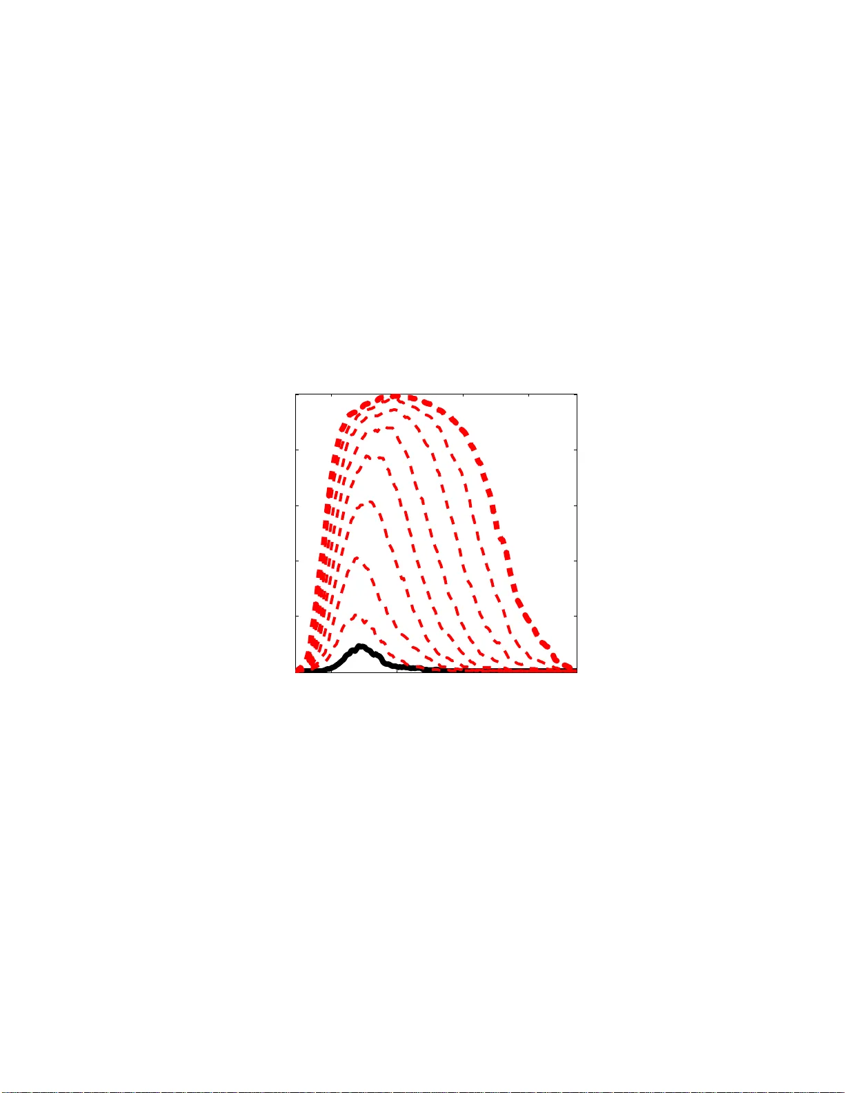
Bolasso: Mo del Consisten t Lasso Estimation through the Bo otstrap F rancis R. Bac h francis.bac h@mines.org INRIA - WILLO W Pro ject-T eam Lab oratoire d’Informatique de l’Ecole Normale Sup ´ erieure (CNRS/ENS/INRIA UMR 8548 ) 45 rue d’Ulm, 752 30 P aris, F ra nce No v em b er 26, 2024 Abstract W e consider the least-square linear regression problem with regular- ization by the ℓ 1 -norm, a problem usually referred to as th e Lasso. In this pap e r, w e presen t a detailed asymptotic analysis of model consistency of the Lasso. F or v ario us decays of the regularizatio n parameter, we comput e asymptotic equiv alents of the probabilit y of correct mo del selection (i.e., v ariable selection). F or a sp ecific rate decay , we show that the Lasso se- lects all the v ariables that should enter th e mo del with probabilit y t ending to one exp onentia lly fast, while it selects all other v ariables with strictly p ositiv e probability . W e show that this prop erty implies that if w e run the Lasso for severa l b o otstrapped replications of a giv en sample, then inters ecting t h e sup p orts of the Lasso b o otstrap estimates leads to consis- tent mo del selectio n. This no vel var iable selectio n algorithm, referred to as the Bolasso, is compared fa vorably t o other linear regressio n metho d s on synthetic data and datasets from the U CI mac hine learning rep ository . 1 In tro duction Regularization b y the ℓ 1 -norm has a ttracted a lot of int er est in recent years in machine learning , statistics and signal pr o cessing. In the context of least-squar e linear regr e s sion, the pr oblem is usually referr ed to as the L asso ( ? ). Much of the early effort has b een dedicated to algor ithms to so lve the optimization problem efficient ly . In particular, the L ars algorithm of ( ? ) allo ws to find the ent ire regulariza tion path (i.e., the se t of solutions for all v alues of the regularization parameters) at the cost of a single matrix inv ersion. Moreov er, a w ell-known justification of the reg ularization by the ℓ 1 -norm is that it leads to sp arse solutions, i.e., loading vectors with many zero s, and th us per forms mo del sele c tio n. Recent works ( ? ; ? ; ? ; ? ) hav e lo o ked pr e c is ely at 1 the mo del consistency of the Lass o, i.e., if we know that the data w ere gener- ated from a spars e loading vector, do es the Lasso actually r ecov er it when the n umber of obser ved data p oints grows? In the case of a fixed num be r of cov ar i- ates, the Lasso do es recover the s pa rsity pa tter n if a nd only if a certain simple condition on the generating cov ariance matrices is verified ( ? ). In particular, in low co rrelation settings, the La sso is indeed co nsistent. How ever, in pre s - ence of strong co rrelations, the L a sso cannot b e co nsistent , s hedding light on po ten tial problems o f such pro cedur e s for v ariable s e lection. Adaptive v er sions where data-dep endent weigh ts ar e added to the ℓ 1 -norm then allow to keep the consistency in a ll situatio ns ( ? ). In this pap er, we first derive a detailed asymptotic analysis of spar s it y pat- tern se lec tio n of the Lasso estimation pro cedur e , that extends previo us analy- sis ( ? ; ? ; ? ), b y fo cusing on a sp ecific decay of the regulariz a tion parameter. W e s how that when the decay is prop ortional to n − 1 / 2 , where n is the n umber of o bs erv ations, then the Lasso will select all the v ariables that should en ter the mo del (the r elev ant v ariables) with pro babilit y tending t o one expo nen- tially fast with n , while it selects all other v ariables (the irr elevant v a riables) with strictly p ositive probability . I f several datas e ts genera ted from the sa me distribution were av ailable, then the la tter prop erty w ould sugg est to consider the intersection of the supp orts of the Lasso estimates for each dataset: all relev ant v a riables w ould alw ays be selected for all datasets, while ir relev ant v ariables would enter the mo dels randomly , a nd int er secting the supp orts from sufficient ly man y differe nt datase ts would simply eliminate them. Ho wev er, in practice, only one dataset is given; but resampling methods such as the b o otstr ap are exactly dedica ted to mimic the av a ilability o f several datasets by resampling from the same unique dataset ( ? ). In this pap er, w e sho w that when using the bo otstrap and intersecting the supp orts, w e a ctually get a consistent mo del es- timate, without the co nsistency condition r equired by the reg ular L a sso. W e refer to this new pro cedur e as the Bolasso ( b o otstrap-e nha nced l east a b s olute s hrink age o per ator). Finally , our Bolasso framework could b e seen as a v oting scheme applied to the suppor ts o f the b o o tstr ap L a sso es timates; howev er, our pro cedure may rather b e consider e d a s a consensus co mb ination sc heme, a s we keep the (largest) subset of v ariables on which al l regr essors agree in terms o f v ariable selection, w hich is in o ur ca s e prov ably consistent a nd a lso a llows to get rid o f a potential additional h yp erpar ameter. The pap er is org anized as follows: in Section 2, we present the asymptotic analysis o f model selection for the La sso; in Section 3, we describ e the B o lasso algorithm as well as its pro of o f mo del consis tency , while in Section 4, we illus- trate o ur results o n synthetic da ta, where the true sparse generating mo del is known, and data from the UCI ma chine learning rep ositor y . Sketc hes o f pro ofs can b e found in Appendix A. Notations F or a vector v ∈ R p , we let denote k v k 2 = ( v ⊤ v ) 1 / 2 the ℓ 2 -norm, k v k ∞ = max i ∈{ 1 ,...,p } | v i | the ℓ ∞ -norm and k v k 1 = P p i =1 | v i | the ℓ 1 -norm. F or a ∈ R , sign( a ) denotes the sign of a , defined a s sign( a ) = 1 if a > 0 , − 1 if a < 0, 2 and 0 if a = 0. F or a vector v ∈ R p , sign( v ) ∈ R p denotes the the vector of signs of elements of v . Moreov er, given a v ector v ∈ R p and a subset I o f { 1 , . . . , p } , v I denotes the vector in R Card( I ) of elements of v indexed by I . Similarly , for a matr ix A ∈ R p × p , A I ,J denotes the submatrix of A comp osed of elements of A whose rows ar e in I and c o lumns a re in J . 2 Asymptotic Analysis of Mo d el Selection for the Lasso In this section, we describ e existing and new asymptotic results regarding the mo del selection capabilities of the Lasso. 2.1 Assumptions W e consider the problem of predicting a resp o nse Y ∈ R from cov ar ia tes X = ( X 1 , . . . , X p ) ⊤ ∈ R p . The only assumptions that we make on the join t distribution P X Y of ( X , Y ) are the following: ( A1 ) The cumulan t ge ner ating functions E exp( s k X k 2 2 ) and E exp( sY 2 ) are fi- nite for some s > 0. ( A2 ) The joint ma trix o f seco nd order momen ts Q = E X X ⊤ ∈ R p × p is inv er t- ible. ( A3 ) E ( Y | X ) = X ⊤ w and v ar( Y | X ) = σ 2 a.s. for some w ∈ R p and σ ∈ R ∗ + . W e let denote J = { j, w j 6 = 0 } the sparsity pattern o f w , s = sign( w ) the sign pattern of w , and ε = Y − X ⊤ w the additive noise. 1 Note that our assumption reg arding cumulan t g enerating functions is s atisfied when X a nd ε hav e compa c t supp ort, and also, when the densities of X and ε hav e light tails. W e consider indep endent and identic al ly distribute d (i.i.d.) d ata ( x i , y i ) ∈ R p × R , i = 1 , . . . , n , sampled from P X Y ; the data are given in the fo r m o f matrices Y ∈ R n and X ∈ R n × p . Note that the i.i.d. assumption, together with ( A1-3 ), are the simplest as- sumptions for studying the a s ymptotic b ehavior of the Las s o; and it is of cour se of in terest to allow mor e g eneral assumptions, in par ticular growing num b er of v ariables p , more genera l random v ariables, etc. (see, e.g., ( ? )), which a re outside the scope of this paper . 2.2 Lasso Estimation W e consider the squar e los s function 1 2 n P n i =1 ( y i − w ⊤ x i ) 2 = 1 2 n k Y − X w k 2 2 and the reg ularization b y the ℓ 1 -norm defined as k w k 1 = P p i =1 | w i | . That is, we 1 Throughout this paper, w e use b oldface fonts for population quantit ies. 3 lo ok at the following Lasso optimization problem ( ? ): min w ∈ R p 1 2 n k Y − X w k 2 2 + µ n k w k 1 , (1) where µ n > 0 is the regular ization par ameter. W e denote ˆ w any globa l minimum of Eq. (1)—it may not b e unique in general, but will with probability tending to one ex p o nent ially fast under a ssumption ( A1 ). 2.3 Mo del Consistency - General Results In this section, we detail the a symptotic be havior o f the L asso estimate ˆ w , b oth in terms of the difference in nor m with the po pula tion v alue w (i.e., reg ular consistency) and o f the sign p attern s ign( ˆ w ), for all asymptotic be haviors of the regular iz a tion parameter µ n . Note that information ab out the sig n pattern includes information abo ut the su pp ort , i.e., the indices i for which ˆ w i is different from zero ; mo reov er, when ˆ w is consistent, consis tency of the sig n pattern is in fact equiv alent to the consistency of the support. W e now consider five m utually exclusive p oss ible situations which explain v arious po rtions o f the re g ularization path (w e assume ( A1-3 )); man y o f these results appear e ls ewhere ( ? ; ? ; ? ; ? ; ? ) but so me of the finer results presented below are new (see Sec tio n 2.4). 1. If µ n tends to infinit y , then ˆ w = 0 with proba bilit y tending to one. 2. If µ n tends to a finite strictly p ositive cons ta nt µ 0 , then ˆ w conv erg es in probability to the unique globa l minimum of 1 2 ( w − w ) ⊤ Q ( w − w ) + µ 0 k w k 1 . Thu s, the estimate ˆ w nev er conv erg es in probability to w , while the sign pattern tends to the one of the previous glo bal minimum, which may or may not be the s ame as the one o f w . 2 3. If µ n tends to zero slow er than n − 1 / 2 , then ˆ w co nv erges in probability to w (regular co nsistency) and the sign pa ttern conv erg es to the sign pa ttern of the glo bal minimum of 1 2 v ⊤ Q v + v ⊤ J sign( w J ) + k v J c k 1 . This sign pattern is equal to the p opulation sign vector s = sign( w ) if and o nly if the following consistency condition is satisfied: k Q J c J Q − 1 JJ sign( w J ) k ∞ 6 1 . (2) Thu s, if E q . (2) is sa tisfied, the probability of cor rect sign estimation is tending to one, and to zero o ther wise ( ? ). 4. If µ n = µ 0 n − 1 / 2 for µ 0 ∈ (0 , ∞ ), then the sign pattern of ˆ w agrees on J with the one of w with pro ba bilit y tending to one, while for all sign patterns c onsistent on J with the one of w , the probability of obtaining this pattern is tending to a limit in (0 , 1 ) (in par ticular strictly po sitive); 2 Here and in the third r egime, we do not tak e into account the pathological cases where the sign pattern of the li mit i n unstable, i .e., the li mit i s exactly at a hinge point of the regularization path. 4 that is, all patterns consis tent on J ar e po ssible with p ositive probability . See Section 2.4 for mo re details. 5. If µ n tends to zero faster than n − 1 / 2 , then ˆ w is consistent (i.e., converges in proba bilit y to w ) but the supp or t o f ˆ w is equal to { 1 , . . . , p } with probability tending to o ne (the signs of v ariables in J c may b e nega tive o r po sitive). That is, the ℓ 1 -norm has no spars ifying effect. Among the five previous regimes, the o nly ones with consistent estimates (in norm) and a sparsity-inducing effect are µ n tending to z e ro and µ n n 1 / 2 tending to a limit µ 0 ∈ (0 , ∞ ] (i.e., potentially infinite). When µ 0 = + ∞ , then we can only hop e for mo del consistent estimates if the consistency c ondition in E q . (2 ) is satisfied. This somewha t disa ppo int ing r esult for the Lass o has led to v arious improv ements on the Lasso to ensure mo del consistency even when E q. (2) is not satisfied ( ? ; ? ). Those a re based on adaptive weigh ts based on the non regularized leas t-square estimate. W e prop ose in Section 3 an alternative way which is based on r esampling. In this pap er, we now consider the sp ecific case where µ n = µ 0 n − 1 / 2 for µ 0 ∈ (0 , ∞ ), where we der ive new asymptotic results. Indeed, in this situation, we g et the correct s igns of the relev ant v ariables (those in J ) with probability tending to one, but we also get all po s sible sig n pa tterns consistent with this, i.e., all other v ariables (those not in J ) may b e no n ze r o with a symptotically strictly p ositive probability . How ever, if we were to rep eat the Lasso estimation for man y datasets o btained from the same distribution, we would o btain for each µ 0 , a set of active v aria bles, all of which include J with probability tending to o ne, but p otentially co ntaining a ll other subsets. By int er s ecting those, we would get exactly J . How ever, this requires multiple co pies of the samples, which a re no t usually av aila ble. Instead, we co nsider bo otstrapp ed samples which exactly mimic the behavior of having mult iple copies. See Section 3 for mor e details. 2.4 Mo del Consistency with Exact Ro ot- n Regularization Deca y In this section we present detailed new results r egarding the pattern c o nsistency for µ n tending to zero exactly at rate n − 1 / 2 (see pro ofs in App endix A): Prop ositio n 1 As su me ( A1-3 ) and µ n = µ 0 n − 1 / 2 , µ 0 > 0 . Then for any sign p attern s ∈ {− 1 , 0 , 1 } p such that s J = sig n( w J ) , P (sign( ˆ w ) = s ) tends to a limit ρ ( s, µ 0 ) ∈ (0 , 1) , and we have: P (sign( ˆ w ) = s ) − ρ ( s, µ 0 ) = O ( n − 1 / 2 log n ) . Prop ositio n 2 As su me ( A1-3 ) and µ n = µ 0 n − 1 / 2 , µ 0 > 0 . Then, for any p attern s ∈ {− 1 , 0 , 1 } p such that s J 6 = sign( w J ) , ther e exist a c onstant A ( µ 0 ) > 0 such that log P (sign( ˆ w ) = s ) 6 − nA ( µ 0 ) + O ( n − 1 / 2 ) . 5 The last tw o prop ositions s ta te that w e get all relev ant v ariables with probability tending to one exp onential ly fast , while we get exactly get all other patterns with probability tending to a limit strictly b etw een ze r o and one. Note that the results that we g ive in this paper a re v alid for finite n , i.e., we could derive actual b ounds on proba bility of sign pattern selections with known constants that explictly dep end on w , Q and P X Y . 3 Bolasso: Bo otstrapp ed Lasso Given the n i.i.d. observ ations ( x i , y i ) ∈ R d × R , i = 1 , . . . , n , given by ma trices X ∈ R n × p and Y ∈ R n , we consider m b o otstr ap replications of the n data po int s ( ? ); that is, for k = 1 , . . . , m , we consider a ghost sample ( x k i , y k i ) ∈ R d × R , i = 1 , . . . , n , g iven by matrices X k ∈ R n × p and Y k ∈ R n . The n pairs ( x k i , y k i ), i = 1 , . . . , n , are sampled uniformly at rando m with r eplac ement from the n original pairs in ( X , Y ). The s ampling of the nm pairs of observ ations is independent. In other words, we defined the distribution o f the ghost sample ( X ∗ , Y ∗ ) by sampling n p oints with replacement from ( X , Y ), and, g iven ( X , Y ), the m ghos t sa mples are independently sa mpled i.i.d. from the distribution of ( X ∗ , Y ∗ ). The a symptotic analys is from Section 2 suggests to estimate the suppo rts J k = { j, ˆ w k j 6 = 0 } of the Lasso e s timates ˆ w k for the b o otstrap samples, k = 1 , . . . , m , and to intersect them to define the Bolasso mo del estimate of the suppo rt: J = T m k =1 J k . Once J is selected, w e estimate w by the unregularized least-squar e fit res tricted to v ariables in J . The detailed algo rithm is given in Algor ithm 1. The algo rithm has only one extra parameter (the nu mber of bo o tstr ap s amples m ). F ollo wing Prop osition 3, log ( m ) should b e chosen growing with n asymptotically slower than n . In sim ulations , w e a lwa ys use m = 1 28 (except in Figure 3 , where w e exactly study the influence of m ). Algorithm 1 Bo la sso Input: data ( X , Y ) ∈ R n × ( p +1) n umber of b o otstra p replicates m regulariza tion para meter µ for k = 1 to m do Generate b o otstra p samples ( X k , Y k ) ∈ R n × ( p +1) Compute La s so estimate ˆ w k from ( X k , Y k ) Compute supp or t J k = { j, ˆ w k j 6 = 0 } end for Compute J = T m k =1 J k Compute ˆ w J from ( X J , Y ) Note that in practice, the Bo lasso es timate ca n be computed simultaneously for a large num ber of reg ularization parameters b ecaus e of the efficiency of the Lars algor ithm (whic h we use in simulations), that allows to find the entire 6 regulariza tion pa th for the La sso a t the (empirical) co st o f a single matrix in- version ( ? ). Th us computational co mplexit y of the Bola sso is O ( m ( p 3 + p 2 n )). The following prop os ition (proved in Appendix A) shows that the previous algorithm leads to consistent model selection. Prop ositio n 3 As su me ( A1-3 ) and µ n = µ 0 n − 1 / 2 , µ 0 > 0 . Then the pr ob abil- ity that the Bolasso do es not exactly sele ct t he c orr e ct mo del, i.e., for al l m > 0 , P ( J 6 = J ) has the fol lowing upp er b ound: P ( J 6 = J ) 6 mA 1 e − A 2 n + A 3 log n n 1 / 2 + A 4 log m m , wher e A 1 , A 2 , A 3 , A 4 ar e strictly p ositive c onstants. Therefore, if log ( m ) tends to infinity slow er than n when n tends to infinity , the Bolasso a s ymptotically s elects with ov erwhelming probabilit y the correct active v ariable, and by re g ular co nsistency of the restricted least-square esti- mate, the co rrect s ign pattern a s well. Note that the previous b o und is true whether the condition in Eq. (2) is satisfied or not, but could b e improv ed on if we supp ose that Eq. (2) is s a tisfied. See Section 4.1 for a detailed compariso n with the Lasso on synthetic examples. 4 Sim ulations In this section, we illustrate the consistency results obtained in this pap er with a few simple simulations on synth etic examples similar to the ones used by ( ? ) and some medium sca le da tasets fro m the UCI machine lea rning rep ository ( ? ). 4.1 Syn thetic examples F or a given dimension p , we sampled X ∈ R p from a norma l distribution with zero mean and c ov ariance matrix genera ted as follows: (a) s ample a p × p matrix G with indep e ndent standa rd nor mal distributions, (b) form Q = GG ⊤ , (c) scale Q to unit diago nal. W e then selected the first Card( J ) = r v ariables and s a mpled non zero loading vect o r s as follows: (a) sample each loading fr om independent standard normal distributions, (b) res cale those to unit magnitude, (c) rescale those by a scaling whic h is uniform at rando m b et ween 1 3 and 1 (to ensure min j ∈ J | w j | > 1 / 3). Finally , w e chose a constant noise level σ equal to 0 . 1 times ( E ( w ⊤ X ) 2 ) 1 / 2 , and the additiv e noise ε is normally distributed with zero mean and v ariance σ 2 . Note that the joint distribution o n ( X , Y ) th us defined satisfies with pr obability one (with resp ect to the sampling of the cov ar iance matr ix) as sumptions ( A1-3 ). In Figure 1, we sampled t wo distributions P X Y with p = 16 and r = 8 relev ant v ariables, one for which the consistency co ndition in Eq. (2) is sa tisfied (left), one for whic h it was no t satisfied (right). F o r a fixed num b er o f sample n = 1 000, we genera ted 256 replications and co mputed the empirica l fr e q uencies of selecting a ny given v aria ble for the L a sso as the reg ularization parameter µ 7 −log( µ ) variable index 0 5 10 15 5 10 15 −log( µ ) variable index 0 5 10 15 5 10 15 Figure 1: Lasso : log-o dd ratios of the pro babilities of selection of each v ariable (white = larg e probabilities, blac k = small pr o babilities) v s. regulariza tion parameter. Consistency c ondition in Eq. (2) satisfied (left) and not sa tisfied (right). −log( µ ) variable index 0 5 10 15 5 10 15 −log( µ ) variable index 0 5 10 15 5 10 15 Figure 2: Bo lasso : log-o dd ratios of the probabilities o f selection of e a ch v ari- able (white = large pro babilities, black = small probabilities) v s. regula r ization parameter. Consistency c ondition in Eq. (2) satisfied (left) and not sa tisfied (right). 8 2 4 6 8 10 12 0 0.5 1 −log( µ ) P(correct signs) 5 10 15 0 0.5 1 −log( µ ) P(correct signs) Figure 3: Bolasso (red, da shed) and Lasso (black, plain): probability of correct sign estimation v s. regular ization para meter. Co nsistency c o ndition in E q. (2) satisfied (left) a nd not satisfied (right). The num be r o f b o o tstra p re plica tions m is in { 2 , 4 , 8 , 16 , 32 , 64 , 128 , 256 } . v aries. Those plots s how the v arious asy mptotic regimes o f the La sso detailed in Section 2. In particular, o n the r ig ht plot, although no µ leads to p erfect selection (i.e., exac tly v ariables with indices less than r = 8 are selected), there is a range where all relev ant v ariables are always selected, while all others are selected with pr obability within (0 , 1 ). In Figure 2, we plot the results under the same co nditions for the Bo lasso (with a fixed nu mber o f bo otstrap replica tions m = 12 8). W e can see that in the Lasso-co nsistent case (left), the Bolasso widens the consistency regio n, while in the Las s o-inconsistent case (rig ht ), the Bolasso “ c r eates” a cons is tency regio n. In Fig ur e 3, we selected the same tw o distributions and compared the pro b- abilit y o f exa ctly selecting the corr ect supp or t pattern, for the Las so, and for the Bo lasso with v arying num ber s of bo otstrap replications (those probabilities are co mputed by av eraging over 25 6 exper imen ts with the same distribution). In Figure 3, we can see that in the Lass o-inconsistent cas e (rig ht ), the Bo- lasso indeed allows to fix the unabilit y of the Lasso to find the corre c t pattern. Moreov er, increa sing m lo oks alwa ys b eneficial; note that althoug h it s e ems to contradict the asymptotic analy s is in Section 3 (which impos es an upp er b ound for co nsistency), this is due to the fact that not selecting (at least) the relev ant v ariables has very low probability and is not observed with only 25 6 replications. Finally , in Figure 4, we compare v arious v ariable selectio n procedur es for linear r e g ression, to the Bo lasso, with t wo distributions where p = 6 4, r = 8 and v arying n . F or all the methods we consider, there is a natura l wa y to select exactly r v ariables with no free par ameters (for the Bolasso , we select the most stable pattern with r elements, i.e., the pattern which cor resp onds to most v alues of µ ). W e can see that the Bolas so outp erforms all o ther v ariable selection metho ds, even in se ttings where the num b er of samples b ecomes of the order of the num b er of v ariables, which r e q uires a dditional theoretical analysis, sub ject of ong oing resear ch. Note in par ticular that we compare with bagg ing of least-squa re reg ression ( ? ) followed by a thresholding of the loading vector, which is another simple w ay of using bo o tstrap sa mples: the Bolasso pr ovides 9 2 2.5 3 3.5 0 0.5 1 1.5 2 log 10 (n) variable selection error 2 2.5 3 3.5 0 2 4 6 log 10 (n) variable selection error Figure 4: Compa rison of several v ariable selection metho ds: La sso (black cir- cles), Bola s so (green cr osses), forward greedy (mag ent a dia monds), thresholded LS estimate (red stars), a daptive Las so (blue pluses). Consistency co ndition in Eq. (2) satisfied (left) and not satisfied (righ t). The averaged (over 32 repli- cations) v ariable selection err or is computed as the s quare distance b etw een sparsity pattern indica tor vectors. a more efficien t w ay to use the extra information, not for usual stabilization purp o ses ( ? ), but directly for mo del selection. Note finally , that the bagging of Lasso estimates requires an additional parameter and is thus not tested. 4.2 UCI datasets The previous sim ulations hav e sho wn that the Bolass o is succesful at p erform- ing mo del selectio n in sy nt hetic examples. W e now apply it to several linear regress io n pr oblems and compar e it to alterna tive metho ds for linear reg ression, namely , ridge reg r ession, Lasso , bagg ing of La sso estimates ( ? ), and a soft ver- sion of the Bola sso (referred to as Bola sso-S), where instea d o f intersecting the suppo rts for ea ch b o o tstrap r e plica tions, we select those which are present in at least 90% o f the b o o tstrap r eplications. In T able 1 , we consider data r an- domly genera ted as in Section 4 .1 (with p = 32, r = 8, n = 64), wher e the true mo del is known to b e comp osed of a sparse loading vector, while in T able 2, we consider reg ression datas ets from the UCI machine learning r ep ository . F or all of thos e, we p erfor m 1 0 re plica tions of 1 0-fold cr oss v alidation and for all methods (which all hav e o ne free regular ization par a meter), we select the b est regulariza tion para meter o n the 100 folds and plot the mean square pr e diction error and its standar d devia tio n. Note that when the gener ating mo del is actually s parse (T able 1), the Bolasso outper forms all o ther mo dels, while in other ca ses (T able 2 ) the Bo lasso is sometimes to o strict in intersecting mo dels, i.e., the softened version works better and is co mpetitive with other methods . Studying the effects of this softened scheme (which is mor e similar to usual voting sc hemes), in par ticular in terms of the po tent ial trade-o ff b etw een go o d mo del selection and low pr ediction error, and under conditions where p is la rge, is the sub ject of ongoing work. 10 T able 1: Compar ison of leas t-square estimation metho ds, data genera ted as describ ed in Section 4 .1, with κ = k Q J c J Q − 1 JJ s J k ∞ (cf. Eq. (2)). Performance is measured through mean squa red prediction error (m ultiplied b y 1 00). κ 0.93 1.20 1.42 1.28 Ridge 8 . 8 ± 4 . 5 4 . 9 ± 2 . 5 7 . 3 ± 3 . 9 8 . 1 ± 8 . 6 Lasso 7 . 6 ± 3 . 8 4 . 4 ± 2 . 3 4 . 7 ± 2 . 5 5 . 1 ± 6 . 5 Bolasso 5 . 4 ± 3 . 0 3 . 4 ± 2 . 4 3 . 4 ± 1 . 7 3 . 7 ± 1 0 . 2 Bagging 7 . 8 ± 4 . 7 4 . 6 ± 3 . 0 5 . 4 ± 4 . 1 5 . 8 ± 8 . 4 Bolasso - S 5 . 7 ± 3 . 8 3 . 0 ± 2 . 3 3 . 1 ± 2 . 8 3 . 2 ± 8 . 2 T able 2: Compariso n of least-square estimation methods, UCI regression datasets. Performance is measured through mean squared prediction error (mul- tiplied by 1 00). Autompg Imp orts Machine Housing Ridge 18 . 6 ± 4 . 9 7 . 7 ± 4 . 8 5 . 8 ± 18 . 6 28 . 0 ± 5 . 9 Lasso 18 . 6 ± 4 . 9 7 . 8 ± 5 . 2 5 . 8 ± 19 . 8 28 . 0 ± 5 . 7 Bolasso 18 . 1 ± 4 . 7 2 0 . 7 ± 9 . 8 4 . 6 ± 21 . 4 26 . 9 ± 2 . 5 Bagging 18 . 6 ± 5 . 0 8 . 0 ± 5 . 2 6 . 0 ± 18 . 9 28 . 1 ± 6 . 6 Bolasso - S 17 . 9 ± 5 . 0 8 . 2 ± 4 . 9 4 . 6 ± 19 . 9 26 . 8 ± 6 . 4 5 Conclusion W e have presented a detailed a nalysis of v ariable selection pro per ties of a b o os- trapp ed version of the Lass o . The mo del estimation pro cedure, referred to as the Bolasso, is prov ably c o nsistent under g e neral assumptions. This work brings to light that p o or v ariable selection results of the Las s o ma y be ea sily enhanced thanks to a simple pa rameter-free resampling pro ce dur e. Our con- tribution also suggests that the use of b o otstrap samples by L. Br eiman in Bagging/ Arcing/Random F orests ( ? ) may hav e been so far slightl y ov erlo o ked and co nsidered a minor feature, while using bo ostrap s amples may actually be a key computational feature in such alg orithms for go o d mo del s election p erfor- mances, and e vent ually go o d prediction perfor mances on real da tasets. The curr ent work could b e extended in v arious ways: fir s t, we hav e focus ed on a fixe d total num b er o f v ariables, and allowing the num ber s of v aria bles to grow is imp ortant in theory a nd in practice ( ? ). Second, the same techn ique can b e applied to similar settings tha n least-sq uare regress ion w ith the ℓ 1 -norm, namely regular iza tion by blo ck ℓ 1 -norms ( ? ) and other losses such as general conv ex cla ssification lo sses. Finally , theo retical and practica l connections could be made with other work o n r esampling metho ds a nd b o osting ( ? ). 11 A Pro of of Mo d el Consistency Result s In this app endix, we give sketc hes of pro ofs for the a symptotic results presented in Section 2 and Section 3. The pro ofs rely on the well-kno wn prope r ty of the Lasso optimization problems, namely that if the sign pattern o f the solution is known, then w e c a n get the solution in closed form. A.1 Optimalit y Conditions W e let denote ε = Y − X w ∈ R n , Q = X ⊤ X / n ∈ R p × p and q = X ⊤ ε/n ∈ R p . First, we can equiv alently r ewrite Eq. (1) as: min w ∈ R p 1 2 ( w − w ) ⊤ Q ( w − w ) − q ⊤ ( w − w ) + µ n k w k 1 . (3) The optimality conditions for Eq. (3) can be written in terms of the sig n pa ttern s = s ( w ) = sign( w ) and the sparsity pattern J = J ( w ) = { j, w j 6 = 0 } ( ? ): k ( Q J c J Q − 1 J J Q J J − Q J c J ) w J + ( Q J c J Q − 1 J J q J − q J c ) + µ n Q J c J Q − 1 J J s J k ∞ 6 µ n , (4) sign( Q − 1 J J Q J J w J + Q − 1 J J q J − µ n Q − 1 J J s J ) = s J . (5) In this pa per , w e fo cus on regular ization pa rameters µ n of the fo r m µ n = µ 0 n − 1 / 2 . The main idea b ehind the r esults is to consider that ( Q, q ) a re dis- tributed accor ding to their limiting distributions, obtained fro m the law of larg e n umbers and the central limit theorem, i.e., Q conv erg e s to Q a .s. and n 1 / 2 q is a symptotically no rmally distributed with mean z ero a nd cov ariance matrix σ 2 Q . When assuming this, Pr op ositions 1 and 2 are stra ightf or ward. The main effort is to make sure that we can safely replac e ( Q, q ) by their limiting distri- butions. The following lemmas give sufficient co nditions for co rrect estimation of the signs of v ariables in J a nd for selecting a given pattern s (note that a ll constants could be expressed in terms of Q and w , deta ils are omitted here): Lemma 1 A ssume ( A2 ) and k Q − Q k 2 6 λ min ( Q ) / 2 . Then sign( ˆ w J ) 6 = sign( w J ) implies k Q − 1 / 2 q k 2 > C 1 − µ n C 2 , wher e C 1 , C 2 > 0 . Lemma 2 A ssume ( A2 ) and let s ∈ {− 1 , 0 , 1 } p such that s J = sign( w J ) . L et J = { j, s j 6 = 0 } ⊃ J . Assume k Q − Q k 2 6 min { η 1 , λ min ( Q ) / 2 } , (6) k Q − 1 / 2 q k 2 6 min { η 2 , C 1 − µ n C 4 } , (7) k Q J c J Q − 1 J J q J − q J c − µ n Q J c J Q − 1 J J s J k ∞ 6 µ n − C 5 η 1 µ n − C 6 η 1 η 2 , (8) 12 ∀ i ∈ J \ J , s i  Q − 1 J J ( q J − µ n s J )  i > µ n C 7 η 1 + C 8 η 1 η 2 , (9) with C 4 , C 5 , C 6 , C 7 , C 8 ar e p ositive c onstants. Then sign( ˆ w ) = sign( w ) . Those tw o lemmas are interesting b e c ause they relate o ptimalit y of cer tain sign patterns to q ua nt ities from which we ca n derive concentration inequalities. A.2 Concen tration Inequalities Throughout the pro ofs, we need to provide upp er b ounds on the following quan- tities P ( k Q − 1 / 2 q k 2 > α ) and P ( k Q − Q k 2 > η ). W e obtain, following standard arguments ( ? ): if α < C 9 and η < C 10 (where C 9 , C 10 > 0 are consta n ts), P ( k Q − 1 / 2 q k 2 > α ) 6 4 p exp  − nα 2 2 pC 9  . P ( k Q − Q k 2 > η ) 6 4 p 2 exp  − nη 2 2 p 2 C 1 0  . W e also co nsider multiv a riate Berry-Esse en ine qualities ( ? ); the probability P ( n 1 / 2 q ∈ C ) can b e es timated as P ( t ∈ C ) where t is normal with mean zero and cov ar iance matrix σ 2 Q . The error is then u n iformly (for a ll conv ex sets C ) upper bo unded by: 400 p 1 / 4 n − 1 / 2 λ min ( Q ) − 3 / 2 E | ε | 3 k X k 3 2 = C 11 n − 1 / 2 . A.3 Pro of of Prop osition 1 By Lemma 2, for any given A , and n la rge enough, the probability that the sign is different from s is uppe rb ounded by P  k Q − 1 / 2 q k 2 > A (log n ) 1 / 2 n 1 / 2  + P  k Q − Q k 2 > A (log n ) 1 / 2 n 1 / 2  + P { t / ∈ C ( s, µ 0 (1 − α )) } + 2 C 11 n − 1 / 2 , where C ( s, β ) is the set of t such that (a) k Q J c J Q − 1 J J t J − t J c − β Q J c J Q − 1 J J s J k ∞ 6 β and (b) for all i ∈ J \ J , s i  Q − 1 J J ( t J − β s J )  i > 0 . Note that here α = O ((log n ) n − 1 / 2 ) tends to zero and tha t we hav e: P { t / ∈ C ( s, µ 0 (1 − α )) } 6 P { t / ∈ C ( s, µ 0 ) } + O ( α ). All terms (if A is la rge enough) are th us O ((log n ) n − 1 / 2 ). This shows that P (sign( ˆ w ) = sign( w )) > ρ ( s, µ 0 ) + O ((log n ) n − 1 / 2 ) where ρ ( s, µ 0 ) = P { t ∈ C ( s, µ 0 ) } ∈ (0 , 1 )–the probability is strictly be tw een 0 and 1 beca use the set and its complemen t hav e non empt y interiors and the norma l distribution has a p ositive definite cov a riance matrix σ 2 Q . The o ther inequality can be proved s imilarly . Note that the consta nt in O ((log n ) n − 1 / 2 ) depends on µ 0 but by carefully considering this dep endence on µ 0 , we could make the inequality uniform in µ 0 as long a s µ 0 tends to zero o r infinit y at most at a logar ithmic s pe e d (i.e., µ n deviates from n − 1 / 2 b y at most a logarithmic factor). Also, it would b e interesting to consider unifor m b ounds on p ortions of the reg ularization path. 13 A.4 Pro of of Prop osition 2 F rom Lemma 1, the probability of not s electing any of the v ariables in J is upper bo unded b y P ( k Q − 1 / 2 q k 2 > C 1 − µ n C 2 ) + P ( k Q − Q k 2 > λ min ( Q ) / 2), which is stra ightforw ardly upp er bounded (using Section A.2) b y a term of the required form. A.5 Pro of of Prop osition 3 In or der to simplify the pro o f, w e made the simplifying assumption that the random v ariables X and ε hav e compact supp orts. Extending the pro ofs to take in to acco unt the loo s er condition that k X k 2 and ε 2 hav e non uniformly infinite cum ulant generating functions (i.e., assumption ( A1 )) can b e do ne with minor changes. The probability that T m k =1 J k is different from J is upper b ounded by the sum o f the following pro babilities: (a) Selecting at least v ariables in J: the pr o bability that for the k - th replication, one index in J is not se lec ted, each of them which is upp er b o unded b y P ( k Q − 1 / 2 q ∗ k 2 > C 1 / 2) + P ( k Q − Q ∗ k 2 > λ min ( Q ) / 2), where q ∗ corresp o nds to the ghost s ample; as common in theoretical analy sis of the b o o tstr ap, w e relate q ∗ to q as follows: P ( k Q − 1 / 2 q ∗ k 2 > C 1 / 2) 6 P ( k Q − 1 / 2 ( q ∗ − q ) k 2 > C 1 / 4) + P ( k Q − 1 / 2 q k 2 > C 1 / 4) (and similarly for P ( k Q − Q ∗ k 2 > λ min ( Q ) / 2)). Because we hav e ass umed that X and ε have compact supp orts, the b o ot- strapp ed v ariables hav e also compact supp or t and we can use conce ntration inequalities (g iven the original v a riables X , and also a fter ex pec ta tion with re- sp e c t to X ). Thus the probability for one b o o tstrap replica tion is upperb o unded b y B e − C n where B and C ar e strictly p o sitive constants. Thus the ov erall co n- tribution of this part is less than mB e − C n . (b) Se lecting at m ost v ar i ables in J: the probability that for all replica- tions, the set J is not exactly selected (note that this is not tight at all since on top of the relev ant v ariables which are selected with ov erwhelming pr obabil- it y , different additional v ariables may be selected for different replications and cancel out when int er secting). Our goal is th us to b ound E  P ( J ∗ 6 = J | X ) m  . By previous lemma s , we hav e that P ( J ∗ 6 = J | X ) is upp er bounded b y P  k Q − 1 / 2 q ∗ k 2 > A (log n ) 1 / 2 n 1 / 2 | X  + P  k Q − Q ∗ k 2 > A (log n ) 1 / 2 n 1 / 2 | X  + P ( t ∗ / ∈ C ( µ 0 ) | X ) + 2 C 11 n − 1 / 2 + O ( log n n 1 / 2 ) , where now, g iven X , Y , t ∗ is nor mally distributed with mean n 1 / 2 q and cov ariance matrix 1 n P n i =1 ε 2 i x i x ⊤ i . The first tw o terms and the last tw o ones are uniformly O ( log n n 1 / 2 ) (if A is large enough). W e then hav e to consider the re ma ining term. W e have C ( µ 0 ) = { t ∗ ∈ R p , k Q J c J Q − 1 JJ t ∗ J − t ∗ J c − µ 0 Q J c J Q − 1 JJ s J k ∞ 6 µ 0 } . By Ho effding’s inequality , we can replace the cov aria nce ma trix that depends on X and Y b y σ 2 Q , at cost O ( n − 1 / 2 ). W e thus hav e to bo und P ( n 1 / 2 q + y / ∈ C ( µ 0 ) | q ) for y normally 14 distributed and C ( µ 0 ) a fixed compact set. Because the set is c o mpact, there exist constants A, B > 0 such that, if k n 1 / 2 q k 2 6 α for α larg e enough, then P ( n 1 / 2 q + y / ∈ C ( µ 0 ) | q ) 6 1 − Ae − B α 2 . Thus, b y tr uncation, w e o btain a bo und of the form: E  P ( J ∗ 6 = J | X ) m  6 (1 − Ae − B α 2 + F log n n 1 / 2 ) m + C e − B α 2 6 exp( − mAe − B α 2 + mF log n n 1 / 2 )+ C e − B α 2 , where we hav e used Ho effding’s inequality to upper b ound P ( k n 1 / 2 q k 2 > α ). By minimizing in closed form with resp ect to e − B α 2 , i.e., with e − B α 2 = F log n An 1 / 2 + log( mA/C ) mA , we obtain the desired inequality . References Asuncion and Newman][200 7 ]UCI Asuncion, A., & Newman, D. (2007). UCI machine lear ning rep ository . Bach][2007]grouplas so B a ch, F. (200 7). Consistency of the gr oup Lasso and mult iple kernel le arning (T ech. rep or t HAL-001 64735 ). http:/ /hal. archives-ouvertes.fr . Bent kus][2 003]b entkus Bentkus, V. (2003). On the dep endence o f the Ber ry– Esseen b ound on dimension. Journal of Statistic al Planning and In fer enc e , 113 , 38 5–402 . Boucheron et al.][2004 ]concentration B oucheron, S., Lug osi, G., & Bousquet, O. (2004). Concentration inequalities. A dvanc e d L e ctur es on Machi ne L e arning . Springer. Breiman][199 6a]bagg ing Breiman, L. (1 996a). Bagging predictors. Mach ine L e arning , 24 , 123 –140 . Breiman][199 6b]stabilizing Breiman, L. (19 96b). Heuristics of instability and stabilization in model selection. A nn. Stat. , 24 , 2350 –238 3. Breiman][199 8]arcing Breiman, L. (1998). Arcing clas s ifier. Ann. Stat. , 26 , 801–8 49. B ¨ uhlmann][2 006]b o os ting B ¨ uhlmann, P . (2 0 06). Bo osting for high-dimensional linear mo dels. Ann. Stat. , 34 , 559– 583. Efron et al.][2 0 04]lar s Efron, B., Hastie, T., Johnsto ne, I., & Tibshira ni, R. (2004). Lea st angle regression. Ann. Stat. , 32 , 407. Efron and Tibshirani][19 98]efron Efron, B., & Tibshirani, R. J. (199 8 ). An intr o duction to the b o otstr ap . Chapman & Hall. F u and Knight][2000]fu F u, W., & Knight, K. (2000). Asymptotics for Lasso- t yp e estimators. Ann. Stat. , 28 , 1356–1 378. Meinshausen and Y u][200 6]yuinfinite Meinshausen, N., & Y u, B. (2006 ). Lasso- typ e re c overy of sp arse r epr esentations for high-dimensio nal data (T ec h. r ep ort 720). Dpt. of Sta tistics, UC Berkeley . 15 Tibshirani][1994 ]lasso Tibshirani, R. (1994). Reg ression shrink age a nd selection via the Lasso. J. Roy . St at. So c. B , 58 , 26 7–28 8. W ainwrigh t][200 6]martin W ain wright, M. J. (2006). Sharp thr eshold s for n oisy and high-dimensional r e c overy of sp arsity u sing ℓ 1 -c onstr aine d quadr atic pr o- gr amming (T ech. rep ort 70 9 ). Dpt. of Statistics, UC Berkeley . Y uan and L in][2 007]yuanlin Y uan, M., & Lin, Y. (2007). On the non-negative garro tte estimator. J. R oy. Stat. So c. B , 69 , 143– 1 61. Zhao and Y u][200 6]Zhaoyu Zhao, P ., & Y u, B. (20 06). On mo del selection consistency of Lasso. J. Mac. L e arn. R es. , 7 , 2541 – 2563 . Zou][2006 ]zou Zo u, H. (2 0 06). The adaptive La sso and its ora c le pro p erties. J. Am. Stat. Ass. , 101 , 141 8–14 29. 16 5 10 15 0 0.5 1 −log( µ ) P(correct signs) 0 5 10 15 0.2 0.4 0.6 0.8 1 −log( µ ) P(correct signs) 6 8 10 12 0 0.2 0.4 0.6 0.8 1 −log( µ ) P(correct signs) 0 5 10 15 0 0.5 1 −log( µ ) P(correct signs) −log( µ ) variable index 0 5 10 15 2 4 6 8 10 12 14 16 −log( µ ) variable index 0 5 10 15 2 4 6 8 10 12 14 16 −log( µ ) variable index 0 5 10 15 2 4 6 8 10 12 14 16 5 10 15 0 0.5 1 −log( µ ) P(correct signs) −log( µ ) variable index 0 5 10 15 5 10 15 2 2.5 3 3.5 0 2 4 6 log 10 (n) variable selection error 88 89 90 91 92 93 94 95 96 97 98 99 00 01 02 03 04 05 06 07 08 0 20 40 60 80 100 120 140 160 Conference/Workshop Year Number of Accepted Papers Historial ICML Locations and Numbers of Accepted Papers Ann Arbor, MI Itaca, NY Austin, TX Evanston, IL Aberdeen, Scotland Amherst, MA New Brunswick, NJ Tahoe, CA Bari, Italy Nashville, TN Madison, WI Bled, Slovenia Stanford, CA Williamstown, CA Sydney, Australia Washington, DC Banff, Canada Bonn, Germany Pittsburgh, PA Corvalis, OR Helsinki, Finland (estimated)