Storms prediction : Logistic regression vs random forest for unbalanced data

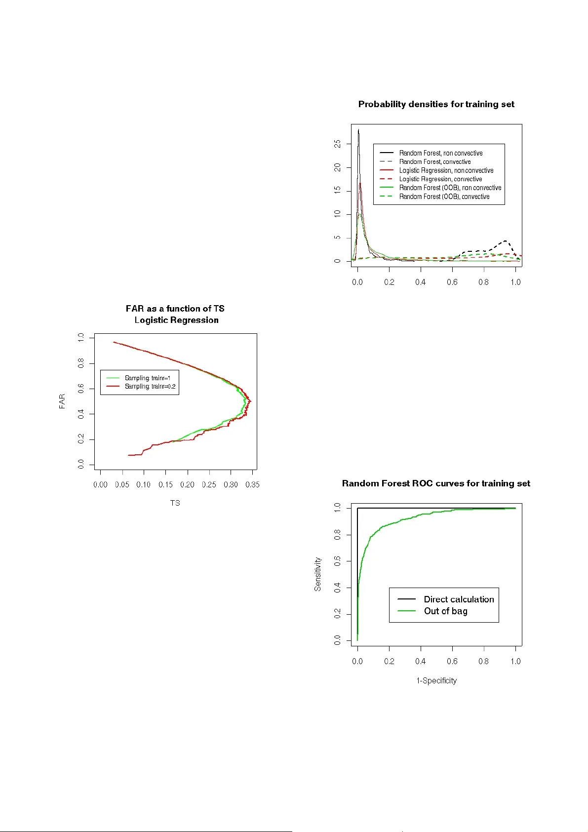
- 1 - ST ORMS PREDICTION: LOGISTIC REG RESSION VS RANDOM FOREST FOR UNBALANCED DA T A Anne Ruiz-Gazen Institut de Ma thématiques de T oulouse and Gremaq, Université T oulouse I, France Nathalie V illa Institut de Mathématique s de T oulouse, Université T oulouse III, France Abstract: The aim of this study is to compar e two supervised classification methods on a crucial meteor ological pr oblem. The data consis t of sa tellite measurements of cloud systems which ar e to be classified eith er in convective or non conv ective systems. Convective cloud systems corr es pond to lightn ing and detect ing such syste ms is of main i mportance for thunderstor m monitori ng and war ning. Becau se the pr oblem is hi ghly unbala nced, we consider specific performan ce criteria and differ ent strategies. This case study can be used in an advanced course of data mining in order to illustrate the use of logistic r egression and random forest on a r eal da ta set with unbalanced classes. Introductio n Predicting storms is a high challenge for the French meteorologi cal group Météo Fra n ce: often, st orms are sudden phenomena th at can cause high damages and lead to stop some human activities. In particular , airports have to be closed during a sto rm and planes have to be taken out of their way to land elsewhere: this needs t o be plane d in order to avoi d airports' overbooking or security difficulties. T o reach this goal, Météo France uses satellites that ke ep a watch on the clouds that stand on France; these clouds are named “systems” and several measurem ents are known about them: some are temperatures, others are m o rphological measurements (volume, height , ...). Moreove r , a “storm network”, base d on measurem ents made on earth, can be used to id entify , a posteriori, systems that ha ve led to storms. Then, a training database has be en built: it contains both satellite measurements and info rmation coming from the stor m network for each considered system. The goal of this paper is to present two statistical approaches in order to di scriminate the convective systems (clouds that lead to a storm) from the non convective ones: a logistic re gressi on is compared to a random forest algorithm. The m ain point of this study is that the data set is extremely unbalanc ed: convective systems repre sent only 4% of the whole data base; therefore, the consequences of such unbal ancing and the strategies developed to overcome it are discussed. The rest of the paper is organized as follows: Section I describes the database. Then, Section II prese nts the methods a nd perform ance criteria t hat are suita ble in this problem. Section III gives some details about the R programs that we used and Sectio n IV presents the results of the study and di scusses them. I. Description of the data set The working dataset was divide d into two sets in a natural way: the first set corresponds to cloud systems observed betw een June and August 2 004 while th e second set corresp onds to syst ems observe d during t he same months in 20 05. So, the 1 1 803 observations made in 2004 are used to build a training sa mple and the 20 998 observ ations made in 2005 are used as a test sample. All the cloud systems are de scribed by 41 numerical variables built from satellite measurements (see the Appendi x for details ) and by their natu re (convective or not ). Moreover , the values of the variables have been recorded at 3 distinct mome nts: all the systems have been observed dur ing at least 30 minutes and a satellite ob servation is made each 15 minutes. The convective sys tems variables have bee n recorded 30 m inutes and 15 m inutes bef ore the first recorded li ghtning an d at the fi rst lightni ng moment. A 30 minutes period als o leading to three di fferent moments has been random ly sampled by Météo France in the trajectories of the non convective systems. A preprocessing that will not be de tailed further has been applied to t he data in order to clean the m up fr om highly correlated variables and from outliers. The reader can find the observations made in 2004 in the file train.csv and the observations m ade in 2005 in the file test.csv . The first line of these files contains the names of the variable and the last column (“cv”) indicates the nature of the data: 1 is set fo r “convective” and 0 for “non co nvective”. The same data can also be found in the R file ruizvilla.Rdata . For the rest of the paper, we will denote X the random vector of the 41 = p satellite measurements and { } 1 , 0 ∈ Y the variable that has to be predicted from - 2 - X (i.e. if the system is convective or not). As most of the obse rved systems are non convective, the database is extrem ely unbalanced: in the traini ng set, 4.06% of the system s are convective and in the test set, only 2.98% of the systems are c onvective. T his very few num ber of convective system s leads to the problem of traini ng a model fr om data ha ving a very few number of observatio ns in the class of interest. II. Methods The models that will be developed further lead to estimate the probability ) 1 ( X Y P = . Th e estimate of this conditional prob ability will be deno ted by ) 1 ( ˆ X Y P = . Usually , g iven these estimates, an observation is classified in class 1 if its estimated probability satisfies 5 . 0 ) 1 ( ˆ > = X Y P . (1) A. Unbalanced data set When the estimation o f ) 1 ( X Y P = has been deduced from an un balanced data set, the met hodology described ab ove could l ead to poor perf ormance res ults (see, for instance, Dupret an d Koda (2001), Liu et al. (2006)). Seve ral simple strategies are commonly proposed t o overcom e this dif ficulty . The first approach consists in re-balancing the dataset. Liu et al. (2006) e xplore several re-balancing schem es both based on downsam pling and on oversam pling. Their experim ents seem t o show that down sampling is a better strate gy . Thus, the traini ng set has bee n re- balanced by keep ing all the observatio ns belonging to the minority class (convective systems) a nd by randomly sampling (without re placement) a given (smaller than the original) number of observations from the majority class (non co nvective systems). Moreover , as suggested by Dupret and Kod a (2001), the optimal re-balancing strategy is not necessarily to downsample the minority class at the same lev el as the majority class. A previous m ining of the dataset (see Section IV , A) leads to choose a downsampling rate equ al to: # Convective / # Non Convect ive = 0.2. The sampled database that was used for training the methods ca n be foun d in the fil e train_sample.csv The second approach to treat the problem of unbalanced database is t o deduce the final decision from the choice of a thr eshol d τ . In equation (1), the threshold is set to 0. 5 but, as em phasized for example in Lemmens and C roux (2006) , this choice is generall y not optimal in the case of unbalan ced datasets. Then, the distribution of the estimates ) 1 ( ˆ X Y P = is studie d for all the observations of the training and test samples and the evolu tion of t he perform ance criterion as a function of the threshold is drawn in orde r to propose several solutions fo r the final decision function. This final decision can be adapted to the goal to achieve, making the balance bet ween a good l evel of recognition for the convective systems and a low level of false alarms. B. Description of the methods W e propose to investigate t wo classification m ethods for the discrimination of convectiv e systems: the logistic regression an d the more recent random forest method. These two approaches have been cho sen for their com plementary properties: lo gistic regression is a well-known and si mple model based on a generalized linear model. On the contrary , random forest is a non linear and non parametric model combining two recen t learning m ethods: the clas sification tree s and the bagging algori thm. A mong al l the recent a dvances in statistical learning, classification trees have the advantage of being very easy to understa nd, which is an important feature for c ommuni cation. Com bined with a bagging scheme, the generalization ability of such a met hod has been prov en to be very i nteresting. In the following, we present more deeply the two methods . Logistic r egression “Logistic regression” is a classification parametric model: a linear model is performed to estimate the probability of an observation to belong to a particular class. Using the notations introduc ed previously , the logistic regressio n estimates the probability ) 1 ( X Y P = by using the f ollowing l inear relation and the maximu m likelihood estimation method: ∑ = + = = = p i j j X 1 X))) | 1 P(Y - (1 X) | 1 P(Y ln( β α (2) with α and p j j ,..., 1 , = β , the parameters to be estimated. A “step by step” iterative algorith m allows to compare a model base d on ' p of the p original variables to any o f its sub-model (with one less variable) and to an y of its top-model (with one more variable): non sign ificant variables are drop ped from the following model and relevant ones are added leading to a final model contai ning a minim al set of relevant variables. This algorithm i s perform ed by the function stepAIC from the R library “MASS” and leads to a logistic regression R object denoted by rl.sbs.opt . This object can be used for prediction by looking at rl.sbs.opt$c oef ficient s which gives t he name of the variables used in t he final model and their corresponding coef ficient β . The Interce p is simply the coefficient α of the model. Using the estimato rs and computing t he model equat ion for a ne w system gives a predicted value S that can be transform ed into a probability to be co nvective by: )) exp( 1 ( ) exp( ˆ S S P + = . - 3 - Random Forest “Random Forest” is a classifi cation or regressi on tool that has been developed rece ntly (Breim an, 2001). It is a combination of tree predictors suc h that each tree is built independently from the ot hers. The method is easy to understand and has proven its ef ficiency as a nonlinear tool. Let us describ e it more precisely . A classification t ree is define d iteratively by a division criterion (node) obtained f rom one of the variables, j x , which leads to the con struction of two subsets in the training sample: one subset contains the observations i that satisfy the condition T x i j < while the other subset contains the observati ons i that satisfy T x i j ≥ ( T is a real num ber which is defined by the algorithm). The choices of the variable and of t he threshold T are automatically built by the algorith m in order to m inimize a heterogenei ty criterion (th e purpose is to obtain two su bsets that are the most homogeneo us as possi ble in te rm of their values of Y ). The growth of the tree is stopped when all the su bsets obtained ha ve homogeneo us values of Y . But, despite its intuitive form, a single classification tree is often not a very accurate classi fication funct ion. Thus, Random Forests are an improvem ent of this classification techni que by aggregating se veral under- efficient classification tre es using a “bagging'” procedure: at each step of the algorithm , several observations and several variables are randomly ch osen and a classification tree is built from this new data set. The final cla ssification de cision is obt ained by a majority vote law on all the classificatio n trees (and we can also deduce an estimati on of the probability of each class by calculating t he proportion o f each decisio n on all the classification trees). When the num ber of trees is large enough, the generalization ability of this algorithm is good. This can be illustrated by the representati on of the “o ut of bag” error which tend s to stabilize to a low value: for each observ ation, the predicted values of th e trees that have not been built using this observation, are calculated. These predictions ar e said “out of bag” because t hey are based on classifiers (trees) for which the considered observation was not selected by t h e bagg ing schem e. Then, by a ma jority vote l aw , a classification “out of bag” is obtained and c ompared to the real class of the observation. Figur e 1. “Out of bag” err or for the training of random for est on the sample train.sample . Figure 1 illustrates the conv ergence of the random forest algori thm: it depicts the e volution of the out -of- bag error as a fu nction of the number of tre es that was used (for the sample data train.sample ). W e can see that, up to about 300 trees, the error stabilizes which indicat es that the obtained ra ndom forest has reached its optimal classification error . C. Performance criteria For a gi ven threshol d τ (see section II A), the performance of a learning me thod can be measured by a confusion matrix which gives a cross-classification of the predicted class (Pred) by the true class (True). In this matrix, the number of hits is t h e number o f observed convective system s that are predicted as convective, th e number of f alse alarms is the number of observed non convective systems that are predicted as convective, the number of misses is the number of observed convective syste ms that are predicted as non convective and the number of cor r ect rejections is the number of observe d non convective systems that are predicted as non convective. Usual performance criteria (see for instance, Hand, 1997) are the sensitivity (Se) which is the nu mber of hits over the num ber of convective system s and the specificity (Sp) which is the number of correct rejections over the number of non convective systems. The well known R OC (receiver operating characteristic) curve plots the sensitivity on the vertical axis against (1 – specificity ) on the horizontal axis for a range of thresh old values. But in this unbal anced problem, such criteria and curv es are not of inte rest. T o illustrate the problem, let us consider the fo llowing small exam ple which is not very dif ferent fr om our data set (T able 1). - 4 - True Pred Convective Non convective T otal Convective # hits # false alarms 500 500 1000 Non convective # misses # correct rejections 0 9 000 9000 T otal 500 9500 10000 Ta b l e 1 For this example, the sensitivity Se=100% and the specificity Sp ≈ 95% are very high but th ese good performances are not really satisfactory from the point of view of M étéo Fra nce. Actuall y , whe n looking at the 1000 detected convective syst ems, only 500 correspond to true convective systems while the o ther 500 correspond to false alarms; this high rate of false alarms is unacceptable practically as it can lead to close airports for wr ong reasons too ofte n. More gene rally , because of the unbal anced problem , the number of correct rejec tions is likely to be very high and so, all the usual perform ance criteria that take into account the num ber of correct rejections are likely to give overoptimistic results. So, in th is paper , the focus will not be on the ROC curve but rather on the following two performance scor es: • the false alarm rate (F AR) : F AR= # false a larms /(# hits + # false alarms) W e want a F AR as close to 0 as possible. Note t hat in the small example, F AR = 50% which is not a good result. • the threat score (TS) : TS= # hits /(# hits + # false alarms + # mi sses) W e want a T S as close to 1 as possible. In the small example, the value of TS=50% which is also not very go od. These perform ance measures can be calcula ted for any threshold τ so that curves can be plo tted as will be illustrated in section IV . Note that for a thresh old near 0 and because the dataset is unbalanced, the number of hits and the number of m isse s are expected to be low compared with the number of false alarm s and so the F AR is e xpected to be near 1 and the TS near 0. When the threshold increases, we expect a decrease of the F AR while the TS will increase until a certain threshold value. For high value of thre shold, if the number of misses increases, the TS will decrease with the threshold, lea ding to a value near 0 when the threshol d is near 1. These dif ferent points will be illustrated in section IV . III. Programs All the programs have been written using R software 1 . Useful inform ation about R program ming can be found in R Development Core T eam (2005). The programs are divided i n to several steps: • a pre -pr ocessing ste p where a sampled database is built. This step is performed via the function rebalance.R which allows 2 inputs, train , which is the data frame of the original training datab ase (file train.csv ) and trainr which is the ratio (# Convective / # Non Con vective) to be found afte r the sampling sche me. The output of this function is a data frame taking int o account the ratio trainr by keeping all the co nvective systems found in train and by downsampling (without replace ment) the non convective systems of train . An example of output dat a is gi ven in fi le train_sample.csv for a sampling ra tio of 0.2. • a training step where the training sampled databases are used t o train a logisti c regression and a ra ndom forest. The logistic r egr ession is performed with a step by step variables selection which lead s to find the most relevant variables for this model. The function u sed is LogisReg.R and uses the library “MASS” provid ed with R programs. It needs 3 inp uts: train.sample is the sampled data frame, train is the original dat a frame from which train.sample has been bu ilt and test is the test data frame (June to August 2005). It provides the t rained m odel (rl.sbs.opt ) and also the probability estimates ) 1 ( ˆ X Y P = for the databases train.sample , train and test , denoted respectively by , prob.train.sample , prob.train and prob.test . 1 Freely available at h ttp://www .r-project.org/ - 5 - The rand om for est is performed by the function RF.R which uses the library “randomForest” 2 . This function has the same inputs and out puts as RegLogis.R but the selected mode l is named forest.opt . It also plots the out-of-ba g error of the method as a function of the number of trees train ed: this plot can help to con trol if the chosen number of trees is large enough for obtaining a stabilized error rate. • a post-pr ocessing step where the performance parameters a re calculated. The function perform.R has 7 inputs: the probab ility estimates calculated during the training step ( prob.train.sample , prob.train and prob.test ), the value of t he variable of interest (convective or not) for the three databases and a gi ven value f or the threshol d, τ , which is named T.opt . By the us e of the libraries “stats” and “ROCR” 3 , the function calculates the confusion matrix for the 3 databases together with the TS and F AR scores associated t o the chosen t hreshold and the Area Under the Curve (AU C) ROC. Moreover , several graphics are built: • the estimated densities for the probability estimates, both for the convective syste ms and the non convective system s; • the histograms of the prob ability estimates both for conv ective and non convective systems for 3 sets of values ([0,0.2], [ 0.2,0.5] and [0.5,1] ); • the graphics of TS and F AR as a function of the threshold togeth er with the graphics of TS versus F AR where the chosen threshold is emphasiz ed as a dot; • the ROC curve. A last function, TsFarComp.R creates graphics that compare the respective TS and F AR for two dif ferent models. The input parameters of this function are: two series of probability estimates ( prob.test.1 and prob.test.2 ), the respective values of the variable of interest ( conv.test1 and conv.test2 ) and a chos en threshold ( T.opt ). The outputs of t his functi on are the graphics of TS versus F AR for both series of probability estimates where the chosen threshold is em phasized as a dot. Finally , the programs Logis.R and RandomForest.R describe a com plete procedure where all these functions are used. In Logis.R the 2 L. Breiman and A. Cutler , available at h ttp://stat- www .ber keley .edu/users/breiman/ RandomForest s 3 T . Sing, O. Sander , N. Beerenwinkel and T . Lengauer , available at h ttp://rocr .bioinf.mpi- sb.mpg.de case where no sampling is made is com pared to the case where a sampling with ra te 0.2 is pre-processed, for the logistic regression. In RandomForest.R , the probability estimates obtain ed for the re-sampled training set train.sample by the use of forest.opt are compared to the out-of-ba g probability estimates. These programs together with the R functions described a bove are provi ded to the reader with the data sets. IV . Results and discussion The previo us program s have bee n used on the traini ng and test databases. In this section, we present so me of the results obtained in the study . In particular , we focus on the un balanced pr oblem and on the com parison between logi stic regression an d random forest according to diffe rent criteria. A. Balancing the dat abase In this section, we consid er the logistic re gression method and propose to com pare the results for dif ferent sampling rates in the non conv ective training databa se. First, let us consider the original training database containing all the record ed non c o nvective systems from June to August 2004. A stepwise l ogistic regression is carried out on this training database as detailed in t he previous se ction (program R egLogis) and predicted probabilities are calcu lated for the training and for the test databases. As already mentioned, once the predicted probab ilities were calculated, the classification decision depe nds on the choice of a thr eshold τ which is crucial. Figure 2. Densities of the p redicted probabilities of the test set for logistic r egression trained on train . Figure 2 plots ker nel density estim ates of the predicted probabilities for the non convectiv e (plain line) and the convective (dotted line) cloud system s for the test database using the train set for train ing. The two densities look very different with a clear mode for the - 6 - non convective systems near 0. T his could a ppear as an encouraging result. However, results are not very good when looking at the F A R and TS. Figur e 3. F AR as a function of TS for logi stic regr ession for the training se t (gr een) and t he test set (red) using the training set train. Figure 3 plots t he F AR as a functio n of TS for diffe rent threshold values from 0 to 1 for t he training database (in green) and for the test database (in red). As expected (see section II), for low values of the threshold w hich correspo nd to high value s of the F AR, the F AR decreases when the TS increases. On t he contrary , for low values of the F AR (which are the interesting ones), the F AR increases when TS increases. As a conse quence, the t hreshold associated with the extreme point on the right of the figure is of interest only if it corresponds to an admissible F AR. On Figure 3, suc h a partic ular threshold is associated with a F AR ≈ 20% and a TS ≈ 35% for t he training dat abase (which is not too bad). But it leads to a F AR ≈ 40% and a TS ≈ 30% for the test database. A F AR of 40% is clearly too hi gh according to Météo France objecti v e but, unfortu nately , in order to obtain a F AR of 20%, we should accept a lowe r TS ( ≈ 20%). Let us now compare the previous results with the ones obtained when considering a sa mple of the non convective systems. Focus is on the test datab ase only . The sampling rate is taken such th at the number of non convective systems is equal to fiv e times the number of convective systems (sampling ratio = 0.2). Figure 4. F AR a s a function of TS for the test set for logistic r egression t rained wit h train (gr een) or train.sample (red) wit h 500 discr etization point s. When looking at Fig ure 4, the TS/F AR curv es look very similar . When sampling, there is no loss in terms of F AR and T S but there is no benefit either . In ot her words, if a th reshold ] 1 , 0 [ 1 ∈ τ is fixed when taking into account all the non conv ective systems in the training database, 1 τ corresponds to som e F AR and TS; it is always possible to find a threshold 2 τ leading to the same F AR and TS for the test database when training on the sampled database. So, the main advantage of s a mpling is that because the training data base is much sm aller , the classification procedure is much faster (especially the stepwise logistic regression) for sim ilar performance. Figure 5. Densities of the probability estimates of the test set for logistic r egression tr ained on train.sample . - 7 - Figure 5 gives the density of th e predicted probabilities for the non convective (plain line) an d the convective (dotted line ) cloud system s for the test dat abase using the train.sample set for training. Comparing Figures 2 and 5 is not in formative because although they are quite different, they correspond to very similar performances in terms of the TS and the F AR. Note that further analysis shows that the sampling ratio 0.2 seems a good com p romise when consideri ng computational speed and performance. Actually , the performance in terms of the F AR and the TS is almost identical when cons idering larger sampling rates while the performance decrea ses a bit for more balanced training databases. As illustrated by Figure 6 which gives a comparison of F A R/TS curves for a sampling ratio of 0.2 and 1, the performance criteria are a littl e bit worse when the training database is completely rebalanced. Also note that , for the random for est algorithm , very simil ar results were obt ained and thus will not be d etailed further . Figur e 6. F AR as a function of TS for logi stic regr ession on train.sample (r ed) and on a training sample with a trainr = 1 (r e-balanced) with 500 discr etization point s. B. Random forest versus logistic regression Here, as e xplained in t he previous section, we focus o n the sampled database train.sample for which the sampling rati o (0.2) appea r s to be a good choice for both logist ic regression an d random fores t. W e now intend to c ompare the two methodol ogies and e xplain their advant ages and dra wbacks. Let us first focus on the comp arison of the densities of the probability estimates obtain ed by both models. Figures 7 and 9 illustrate this comparison for th e training ( train.sample ) and the test sets. The first salient thing is the differe nce between direct calculation of the probability estimates for the random forest model and the out-of-bag calculatio n for the training set: Figure 7 shows distinct densities, both for convective and non convec tive systems (black and green curves). Figure 7. Densities of the pr oba bility estimates for both ran dom for est and logi stic r egress ion on t he training set. The probability estimates for the random forest method are given for “out -of-bag” values (green) and for direct estimation from the final model (black). This phenom enon is bett er explaine d when loo king at the respective ROC curves ob tained for random forest from the probability estimates calculated from the whole model and those calcula ted by t he out-o f-bag scheme (Figure 8). Figure 8. ROC curves for Ra ndom Forest for the training set built from the pr oba bility estimates directly calcul ated by the use of the chosen model (black) and from the out-of-bag pr obability estimates (gree n). This figure shows that the ROC curve built from the - 8 - direct calculation of the probability estimates (b lack) is almost perfect whereas the one obtained from the “out- of-bag” probab ility estimates is much worse. This illustrates well that random forests overfit the training set, giving an almost perfect pre diction for its observations. As a con sequence, the prob ability densities built directly from the training set (b lack in Figure 7) have to be interpreted with care: although they seem to look better than the logistic regression ones, they c ould be m isleading about th e respective performances of the two m odels. Figure 9. Densities of the pr o bability estimates on the test set for r andom fore st and logistic regr ession. Moreover , looking at Figure 9, logistic regression seems to better discriminate the two families of probability estimates (for convectiv e systems and non convective system s) than the random forest met hod for the test set. But, this conclusion should also be taken with care, due to possi ble scaling dif ferences. T o provide a fairer compa rison, the gr aph of F AR versus TS is gi ven in Figur e 10 for bot h random forest (black) and lo gistic regression (re d). T he first remark from this gra phic is that the perform ances of both models are rather poo r: for a F AR of 30%, which seems to be a maxim um for Météo France, the optim a l TS is about 25-30% only . Focusing on the comparison between random forest and logistic regression, things are not as easy as t he comparison of probability densities (Figure 9) cou ld leave to believe. Actually , the optimal model strongly depends on the objectives: fo r a low F AR (between 15- 20%), the optimal model (that h as the highest TS) is logistic regression. But if higher F A R is allowed (20- 30%), then random fores t should be used f or prediction. Figur e 10. F AR as a function of TS for the test set (500 discretization points). These conclusions give t he idea that the two sets of densities can be simply re-scaled one from the other (approximately). Figure 1 1 explains in details what happens: in this figure, th e density of the prob ability estimates for the logistic regression is estimated, as in Figure 7, but the densities for the rando m forest method have been re-scal ed. Figure 1 1. Rescaled probability densities for the test set (details about it s definition are given in the text). More precisely , these probability estimates have been transformed by the following function: ⎩ ⎨ ⎧ > − ≤ = 5 . 0 if ) 1 ( - 1 5 . 0 if ) ( x x x x x x x β α ϕ where 6 . 0 ) 6 . 0 1 ( 2 + − = x x α and - 9 - 3 3 10 ) 1 )( 10 1 ( 2 − − + − − = x x β . Clearly , this simple transformation does not affect the classification ability of the method (the ranking of the probabilities is not modified) and shows that random forest and logistic regression have very close ability to discriminat e the two po pulations of clouds. Moreover , a single rank test (paired Kendall test) proves that th e ranking of t he two m ethods are stro ngly simi lar , with a p-value of this test is less than 1E-15. V . Conclusion Several concl usions can be drive n from this study: the first one is that unbalan ced data lead to specific problem s. As was proven i n this paper , results obtai ned with this kind of da ta should be taken with care. Usual misclassification errors may be irrelevant in this situation: ROC curv es can lead to overoptimistic interpretations while comparison of predicted probability dens ities can lead to misunderstanding. In this study , where a low false alarm rate is one of the main objectives, curves of F AR versus TS are particularly interesting fo r interpretation and comparisons. Another interesting aspect of this study is th e surprisingly comparable results of the simple logistic regression compared to the popular and m ore recently developed r andom forest method. Hand (200 6) already argued that the most recen t classification m ethods may not improve the results ov er standard methods. He points out the fact that, e specially in the case of mislabellings in the database , the gain made by recent and sophisticated st atistical methods ca n be marginal. Both, the way th e database has been bu ilt (by merging satellites sources and storm network records) and the poor perform ance results obtained with several classification methods, tend to suspect m islabellings. As the logistic regression is a faster method than the random forest and because it leads to simple interpretati on of the e xplanatory variables, i t can be of interest for meteorologists. Finally , to better analyse the performances of the proposed methods, m ore information c ould be added to the database. For instance, a storm proximity index could indicate if false positive systems are closer to a storm than true positive ones. Acknowledgments W e wou ld like to thank Thibault Lau rent and Houcine Zaghdoudi for cl eaning the origi nal database and helping us in the practical aspects of this study . W e are also grateful to Y ann Guillou and Frédéric Au tones, engineers at M étéo France, T oulouse, fo r giving us the opportunit y to wor k on this project an d for pr oviding the databases. References Breiman, L. 2001. Random Fo r ests. Machine Learning, 45, 5-32. Dupret, G . and Koda, M. 200 1. Bootstra p re-sampl ing for unbalanced data in supervised learni ng. Eur opean Journal of O perational Re search 134(1): 141-156. Hand, D. 1997. Constru ction and Assessment of Classification Rules. W iley . Hand, D. 2006. Classifier T ech nology and the Illusion of Progress. S tatistical Science. 21(1), 1- 14. Lemmens, A. and Croux, C. 2006. B agging a nd boosting classification trees to predict churn . Journal of Marketing R esear ch 134(1): 1 41-156. Liu, Y ., Chawla, N., Harper , M., Shriber g, E. and Stolcke, A. 2006. A study in machine learning for imbalanced da ta for sentence bounda r y detecti on in speech. Computer Speech and Language 20(4): 468- 494. R Developm ent Core T eam 2005. R : a lang uage and envir onment for statistical computing. R Foundation for St atistical Com puting, V ienna , Austria. Correspondenc e: ruiz@cict.fr (Anne Ruiz-Gazen) and nathalie.villa@math.ups-tlse.fr (Nathalie V illa) - 10 - Appendix: variables definition In this section, we describe the explanatory variables that were collected by satellite in order to explain storms. In the follo wing, T will design the instant of the storm (for convective systems) or the last sam p led instant (for no n convective systems). Δ t will be the difference of time between t w o consecutive records (15 minutes). T emperature variables • TsBT.0.0 is the threshold temperature at T recorded at the basis of the cloud tower . • toTmoyBT.0.0 is the mean rate of variation of the mean temperature between T and T - Δ t at the basis of the cloud tower . • Tmin.0.30 is the minimal temperature at T -2 Δ t recorded a t the top of the cloud to wer . • toTmin.0.0 , toTmin.0.15 and toTmin.0.30 are the minimal temperatures at T recorded at the top of the cloud tower ( toTmin.0.0 ) or the mean rate of variation of the minim al temperature between T and T - Δ t ( toTmin.0.15 ) or between T - Δ t and T -2 Δ t ( toTmin.0.30 ) recorded at the top of the tower of the cloud. • stTmoyTminBT.0.0 and stTmoyTminBT.0.15 are the dif f erences between the mean tem perature at the basis of the cloud tower and the m inimal temperature at the top of the cloud tower at T ( stTmoyTminBT.0.0 ) or at T - Δ t ( stTmoyTminBT.0.15 ) . • stTmoyTminST.0.0 , stTmoyTminST.0.15 and stTmoyTminST.0.30 are the dif f erences between mean temperature and the minimal temperature at the t op of the cloud tower at T ( stTmoyTminST.0.0 ), at T - Δ t ( stTmoyTminST.0.15 ) or at T -2 Δ t ( stTmoyTminST.0.30 ). • stTsTmoyBT.0.0 , stTsTmoyBT.0.15 and stTsTmoyBT.0.30 are the dif ferences between the mean tem perature and the threshold tem perature at the basis of the cloud tower at T ( s tTsTmoyBT.0.0 ), at T - Δ t ( stTsTmoyBT.0.15 ) or at T -2 Δ t ( stTsTmoyBT.0.30 ). • stTsTmoyST.0.0 , stTsTmoyST.0.15 and stTsTmoyST.0.30 are the dif ferences between the mean tem perature at the top of the cloud towe r and the threshol d temperature at the basis of the cloud tower at T ( stTsTmoyST.0.0 ), at T - Δ t ( stTsTmoyST.0.15 ) or at T -2 Δ t ( stTsTmoyST.0.30 ). Morphological variables • Qgp95BT.0.0 , Qgp95BT.0.15 and Qgp95BT.0.30 are 95% quantiles o f the gradients (d egrees per kilometer) at the basis of the cloud t ower at T, T - Δ t and T -2 Δ t . • Qgp95BT.0.0.15 and Qgp95BT.0.15.30 are the change rates between Qgp95BT.0.0 and Qgp95BT.0.15 and between Qgp95BT.0.15 and Qgp95BT.0.30 (calculated at the prep rocessing sta ge, from the original variable). • Gsp95ST.0.0.15 and Gsp95ST.0.15.30 are the change rates between the 95% quantile of th e gradients (degrees per kilometer) at the top of the cloud tower between T and T - Δ t and between T - Δ t and T -2 Δ t (calculated, as a pre-processing, from the ori ginal varia bles). • VtproT.0.0 is the volume of the cloud at T . • VtproT.0.0.15 and VtproT.0.15.30 are the change rates of the volumes of the cloud between T and T - Δ t and betw een T - Δ t a n d T -2 Δ t (calculated, as a pre- processing, from the original variables). • RdaBT.0.0 , RdaBT.0.15 and RdaBT.0.30 are the “aspect ratios” (ra tio between the largest axis and the smallest axis of the ellipse that models the cloud ) at T, T - Δ t and T -2 Δ t . • RdaBT.0.0.15 and RdaBT.0.15.30 are the change rates of the aspect ratio between T and T - Δ t and between T - Δ t and T -2 Δ t (calculated, at the preprocessing stage, from the original variables). • SBT.0.0 and SBT.0.30 are the surfaces of the basis of t he cloud towe r at T and T -2 Δ t . • SBT.0.0.15 and SBT.0.15.30 are the change rates of the surface s of the basis of t h e cloud tower be tween T and T - Δ t and between T - Δ t and T -2 Δ t (calculated, at the preprocessing stage, from the original variables). • SST.0.0 , SST.0.15 and SST.0.30 are the surfaces of the top of the cloud tower at T, T - Δ t and T -2 Δ t . • SST.0.0.15 and SST.0.15.30 are the change rates of the surfaces of the top of the cloud tower be tween T and T - Δ t and between T - Δ t and T -2 Δ t (calculated, at the preprocessing stage, from the original - 11 - variables).