Joint Beamforming for Multiaccess MIMO Systems with Finite Rate Feedback

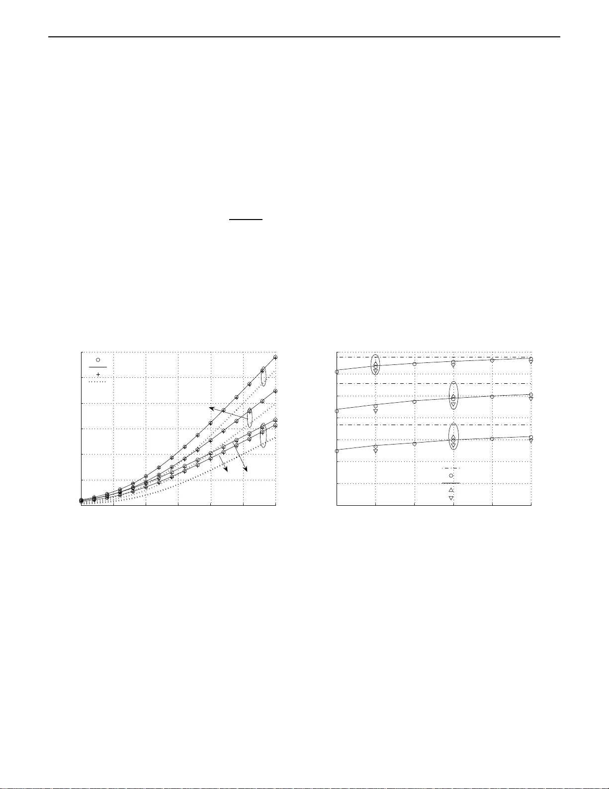
1 Joint Beamforming for Multiaccess MIMO Sy stems with Finite Rate Feedback ∗ W ei Dai † , Brian C. R ider †† and Y oujian(Eugene) Liu † † Department of Electrica l and Computer Engineering, Univ ersity of C olorado at Boulder †† Department of Mathematics, Univ ersity of Colorado at Boulder Abstract This paper considers mu ltiaccess multiple-inpu t multiple-ou tput (MI MO) system s with finite rate feed back. The goal is to understand how to efficiently em ploy the gi ven finite feedback resource to maximize the sum rate by characterizin g the perf ormanc e analy tically . T o wards th is, we propo se a jo int quan tization and feedback strategy: the base station selects the stronge st users, jointly qu antizes their stron gest eigen -chann el vectors and b roadcasts a common feedb ack to all the users. This joint strategy is different fro m an individual stra tegy , in which qu antization and feedb ack ar e p erform ed across u sers indepen dently , a nd it improves u pon the individual strategy in the sam e way that vector quantization improves upon scalar quantization. In our proposed strategy , the effect of user selection is analyzed by extreme order statistics, while th e ef f ect o f jo int q uantization is quantified by what we term “the composite Grassman n manif old”. The achiev ab le su m rate is then estimated by rand om m atrix theo ry . Due to its simple impleme ntation and solid performance an alysis, the propo sed sche me provides a benchmark for multiaccess MIMO systems with finite rate feedback . I . I N T R O D U C T I O N This paper considers m ultiaccess system s, corresponding to the u plink of cellul ar systems , where both the base station and the multiple users are equipped with multipl e antennas. Multi ple antenna systems , also known as multipl e-input multip le-output (MIMO) system s, provide significant benefit over s ingle antenna systems in terms of increased spectral efficienc y and/ or reliability . The full potential of MIMO though requires perfect channel state information (CSI) at bot h the transmitter and the receiver . While i t is often reasonable to assume that the recei ver has perfect CSI through a pilot signal, assuming perfect CSI at the transmitter (CSIT) is typ ically unrealisti c. In m any practical systems, the transm itter obtains CSI through a finite rate feedback from the recei ver . Not e that a wireless fading channel may have infinitely many channel states, and a finite rate feedback imp lies that CSIT is imperfect. One expects a performance degradation, and here we focus on the quantitative ef fect of finite rate feedback and the corresponding design. Insight from s ingle us er MIM O s ystems wi th finite rate feedback proves beneficial. Single user s ystems are similar to mult iaccess system s in th e sens e th at there is only one receiv er in bot h systems. The receiv er knows the channel states perfectly and h elps transmit ters adapt their signals to m aximize through put. The essential differe n ce between these two types of systems lies i n t he modes of antenna cooperation. In single user MIMO systems, all the transmit antenn as are able t o cooperate in s ending a given message. In multiaccess systems, diffe rent users hav e independent messages, and transmit antennas belonging to on e user cannot aid th e transmission of another user’ s message. Due to t his additional con straint, the analy sis and design of mult iaccess s ystems becomes more complicated. Still , we will borro w in sight from single user syst ems to simpli fy the design of multiaccess systems . F o r singl e user MIMO s ystems, strategies to maximize throughput with p erfect CSIT and without CSIT are deriv ed and analyzed in [1]. When only finite rate feedback i s av ailable, the focus has moved t ow ard the development of su boptimal strategies as a simp lification. T he dominant approach is based on power o n/off strategy , in which a data st ream is ∗ This work is supported by NSF Grants CCF-0728955, ECCS -0725915 , DMS-050568 0 and Thomson Inc. Part of content was presented in Allerton C onf. on Communication, Control, and C omputing, 2005. T echnical Report either tu rned on with a pre-determined constant power or turned of f (zero power). Systems with only one stream are consi dered in [2]–[4]. Systems with multiple ind ependent st reams are in vestigated in [5]–[11]. It appears that power on/off strategy is near optim al compared to t he opti mal power water -filling allocation [10]. W e aim t o understand how to efficiently employ the giv en finite feedback resource to m aximize the sum rate by characterizing performance analytically . The full multi access M IMO problem sti ll appears behind reach mathematically and is left for the future. In this paper , we prop ose a subop timal strategy by borrowing insight and methods from single us er systems. Specifically , the base station selects the strongest users, jointly quantizes their strongest eigen-channel vectors and broadcasts a common feedback to all the users. Instead of d esigning a specific quantization code book, we show that the performance of a random code b ook is optimal in probabilit y . After receiving feedback in formation, a selected on-user employ power on/off strategy and transmit alon g the beamforming vector selected by the feedback. Here, joint quantization and feedback are employed based on the pl ain fact t hat vector quanti zation is b etter t han scalar quantization [12, Ch. 1 3]. (The precise gain wi ll be verified empirically .) It i s also worth noti ng that, as we shall discus s in Section IV and V, antenna selectio n can be viewed as a simplified version o f the proposed s cheme. This approach differs from the ongoing research for broadcast channels (BC) with finit e rate feedback. While there is a well known duality between broadcast and multiaccess system s [13], this dualit y requires full CSI at bot h the t ransmitters and t he receivers and is not av ailabl e when onl y partial CSIT is provided. When CSIT i s av ailable only throu gh finite rate feedback, broadcast syst ems suffer from th e so called interference domin ation phenomenon [14], [15]. The major ef fort in research is to lim it the interference among users. Sharif and Hassibi select the near orthogonal channels wh en the number of us ers is suffi cient ly large [14], [15]. As the n umber of users i s comparable to the n umber of antennas at th e base station, Jindal sh ows t hat the feedback rate sho uld be proport ional to signal-to -noise ratio (SNR) if the number of users turned on is fixed [15], while we show that the number of us ers s hould be adapt to the SNR if the feedback rate is given [16]. Howe ver , the int erference domination phenomenon does not appear in multiaccess systems. Note that the search of near ortho gonal channel s suf fers from exponential increasing complexity . Neither the results nor the methods for broadcast systems can be directly appl ied to th e pro blem di scussed i n this paper . Though the s trategy in this paper is relative l y simple, the corresponding p erformance analysis is nontrivial. Our main analytical result is an upper bound on the sum rate, which to our knowledge is the best to date. The effect of user/antenna selecti on is analyzed by extreme order statisti cs, and the ef fect of eig en-channel vectors j oint q uantization i s quantified via the compos ite Grassmann manifol d . Interestingly , the comp licated ef fect of imperfect CSIT and feedback is ev entu ally described by a si ngle constant, which we t erm the power efficiency factor . Successful e valuation of the power ef ficiency factor enables us characterize the upper bound on the su m rate. The anticipated goodness o f the upp er b ound is supported by sim ulation of sever al systems with a large range of SNRs. The rest of th is paper is organized as follows. The general model for multiaccess systems with finite rate feedback is described in Section II. The mathematical results de veloped for performance analysis are assembled in Section III. The antenna selection strategy is analyzed in Section IV -A. Then a subopti mal strategy is proposed and analyzed i n Section IV -B. In Section V, simulati on results are presented and discussed. Finally , Section VI summarizes the paper . I I . S Y S T E M M O D E L Assume that th ere are L R antennas at the base station and N users communicati ng with the base station. Assume that the user i 1 has L T ,i transmit antennas 1 ≤ i ≤ N . T hroughout we will s et L T , 1 = · · · = 1 When a user joins the multiaccess system, a unique index is assigned and keeps constant. A user in a multiaccess system is aware of the corresponding index. 2 T echnical Report L T ,N = L T . The signal transmiss ion model is Y = N X i =1 H i T i + W , where Y ∈ C L R × 1 is the recei ved signal at the base station, H i ∈ C L R × L T is the channel state matrix for user i , T i ∈ C L T × 1 is the transmit ted Gaussian signal vector for user i and W ∈ C L R × 1 is the addi tiv e Gaussian no ise vector with zero mean and covariance matri x I L R . W e assume the Rayleigh fading channel model: the entries of H i ’ s are independent and identi cally distributed (i.i.d.) circularly symmetri c com plex Gaussian variables wit h zero mean and unit v ariance ( C N (0 , 1) ), and H i ’ s are i ndependent across i . W e furt her assume that there exists a feedback link from the base station to the users. At the beginning of each chann el use, t he channel st ates H i ’ s are perfectly estim ated at the recei ver (the base station). This assum ption is valid i n practice since most com munication standards allow the receiv er to learn t he channel states from pilot si gnals. A commo n message, which i s a function of the chann el states, i s sent back to all users through the feedback link. W e assume t hat th e feedback link is rate limi ted and error- free. Th e feedback directs the users to choose their Gaussian signal cov ariance matrices. In a mu ltiaccess communication syst em, different users cannot c o operate in terms of information message, leading to E h T i T † j i = 0 for i 6 = j . Let T = h T † 1 · · · T † N i † be the overall t ransmitted Gauss ian signal for all users and Σ , E  TT †  be the overall signal covariance m atrix. Th en Σ is an N L T × N L T block d iagonal matrix whose i th diagonal block is the L T × L T cov ariance matrix E h T i T † i i . Let H = [ H 1 H 2 · · · H N ] be the overall channel state matrix. An extension of [17] shows that t he opt imal feedback strategy is to feedback the i ndex of an appropriate cova riance m atrix, which is a functi on of current channel state H . Last, ass ume t hat t here i s a cov ariance matrix codebook B Σ = { Σ 1 , · · · , Σ K B } (wit h finite size) declared to both the base station and the users, where each Σ k ∈ B Σ is the overall signal cov ariance matrix with block diago nal structure just described, and K B is the size of the codebook. The feedback fun ction ϕ is a map from  H ∈ C L R × N L T  onto the ind ex set { 1 , · · · , K B } . Subjected to this finite rate feedback constraint |B Σ | = K B and the aver age total transmiss ion power constraint E H  tr  Σ ϕ ( H )  ≤ ρ, the sum rate of the optimal feedback st rategy is given by sup B Σ sup ϕ ( · ) E H  log   I L R + HΣ ϕ ( H ) H †    . (1) Here, since only sym metric syst ems are concerned, the total power constraint ρ is equiva l ent to individual power constraint ρ/ N . Note that the opt imal strategy inv olves two coup led optimi zation problems . It is diffic ul t, if not impossi ble, to find its explicit form and performance. Instead, we shall study tw o subopti mal strategies and characterize th eir s um rates in Section IV. I I I . P R E L I M I N A R I E S This s ection assembles math ematical results required for later analysis. The reader may proceed directly to Section IV for the main engineering result s. 3 T echnical Report A. Or der Statisti cs for Chi-Squar e Random V ariables Define X i = P L j =1 | h i,j | 2 where h i,j 1 ≤ j ≤ L, 1 ≤ i ≤ n are i .i.d. C N (0 , 1) . Then each X i has a Chi-square d istribution with probabi lity densit y functio ns (PDF) f X ( x ) = 1 ( L − 1)! x L − 1 e − x . Denote the corresponding cum ulative distribution function (CDF) by F X ( x ) . Next i ntroduce the order statistics for these variables: that is t he non-decreasing l ist X (1: n ) ≤ X (2: n ) ≤ · · · ≤ X ( n : n ) connected with each realization. Here, the sub script ( k : n ) indicates that X ( k : n ) is the k th minima. (W e follow the con vention of [18].) Note of course that ties occur wi th probabi lity zero and can be broken arbitrarily . W e will need th e following, which is proved i n Appendix B. Lemma 1 : W ith the notati on set out above, for any fixed positive i nteger s it hol ds lim n → + ∞ E  P s k =1 X ( n − k +1: n ) − sa n b n  = s µ 1 + 1 − s X k =1 1 k ! , (2) where a n = inf  x : 1 − F X ( x ) ≤ 1 n  , b n = P L − 1 i =0 L − i i ! a i n P L − 1 i =0 1 i ! a i n , and µ 1 = R + ∞ −∞ xde − e − x may be comput ed num erically . The lim iting result in expectation imm ediately provides t he following approximati on for a fixed s : E " s X k =1 X ( n − k +1: n ) − sa n # = sb n µ 1 + 1 − s X i =1 1 i ! (1 + o (1)) . (3) The shape of F X guarantees that a n and so b n are finite for any fixed n but tend to i nfinity and one respectiv ely wi th th is parameter . B. Condition ed Eigen values of the W i shart Matr ix Let H ∈ L n × m be a random n × m matrix whose entries are i.i.d. Gaussi an random variables with zero mean and unit variance, w here L is either R or C . Througho ut, we refer to H as the standard Gauss ian random matrix. Let λ 1 ≥ λ 2 ≥ · · · ≥ λ n be the ordered eigen values of W = HH † ( W is W ish art distributed [19]). This subsection takes up an estimate of E [ λ 1 | tr ( W )] , where tr ( · ) is the usual matrix trace. In particular , while a closed formula for t his o bject would be rather in volved, we may use random matrix theory to obtain an approxi mation. The first ingredient is the following. Lemma 2 : Let H ∈ L n × m (w .l.o.g. n ≤ m ) 2 be a standard rando m Gauss ian matrix. L et λ 1 ≥ λ 2 ≥ · · · ≥ λ n be the ordered eigen values of W = HH † . Then E [ λ i | tr ( W ) = c ] = ζ i c, where ζ i = E [ λ i | tr ( W ) = 1] . (4) , (5) 2 If n > m , E ˆ λ i | tr ` HH † ´ = c ˜ = 0 for i > m and E ˆ λ i | tr ` HH † ´ = c ˜ = ζ ′ i c for i ≤ m , where ζ ′ i := 1 c E ˆ λ i | tr ` H † H ´ = c ˜ . The calculation of ζ ′ i for i ≤ m is included in T heorem 2 as well. 4 T echnical Report β = 1 if L = R or β = 2 if L = C , and | ∆ n ( λ ) | = Q n i 0 , lim ( n,K ) →∞ Pr  D ( C rand ) > mp 2 − 2 β mp r + ǫ  = 0 . 7 T echnical Report The proof of this theorem follows from tho se in [11, Theorem 3] and is omitted here. This t heorem provides a form ula for the distortion rate function at finite n and K : D ∗ ( K ) = 2 mt Γ  2 mt  Γ 2 mt  m t 2 + 1  Γ 2 t  t 2 + 1  c − 2 t n,p,p , β 2 − 2 log 2 K mt ! (1 + o (1)) . ( 9 ) By the asymptotic o ptimality of random codes, we have empl oyed random codes for our analysi s, and approximate the correspon ding disto rtion rate function by ignoring the high er order terms behind (9). D. Calculation s Related to Composit e Grassmann Ma trices A compos ite Grassmann matri x P ( m ) is a generator matrix generatin g P ( m ) ∈ G ( m ) n,p ( L ) , and w e denote t he set of com posite Grassm ann m atrices by M ( m ) n,p ( L ) . A composite Grass mann m atrix P ( m ) = [ P 1 · · · P m ] ∈ M ( m ) n,p ( L ) generates a plane P ( m ) = ( P 1 , · · · , P m ) ∈ G ( m ) n,p ( L ) , where P 1 , · · · , P m are the generator m atrices for P 1 , · · · , P m respectiv ely . Note that t he generator matrix P i for a pl ane P i ∈ G n,p ( L ) is not unique. The composite Grassmann matrix P ( m ) ∈ M ( m ) n,p ( L ) generatin g P ( m ) ∈ G ( m ) n,p ( L ) is not unique either: let U ( m ) is an arbitrary pm × pm bl ock diagonal matrix whos e i th ( 1 ≤ i ≤ m ) di agonal block i s a p × p ortho gonal/unitary m atrix (w .r .t. L = R / C respectively); if P ( m ) generates P ( m ) , then P ( m ) U ( m ) generates P ( m ) as well. V i e w M ( m ) n,p ( L ) as a Cartesian product of m many M (1) n,p ( L ) . Then the isotropic measure µ on M ( m ) n,p ( L ) is simply the product o f Haar measure on each composed M (1) n,p ( L ) ’ s. W e say a P ( m ) ∈ M ( m ) n,p ( L ) i s isotro pically d istributed if t he corresponding prob ability measure is the isotropic measure µ . Note now that we are in terested in quantifying E  log   I + c P ( m ) P ( m ) †    , for a const ant c ∈ R + and isotropically di stributed P ( m ) ∈ M ( m ) n, 1 ( C ) . The asy mptotic behavior of thi s quantify is d eri ved b y random matrix theory techniques. Theor em 3: Let P ( m ) ∈ M ( m ) n, 1 ( C ) be i sotropically di stributed. For all posi tiv e real num bers c , as n, m → ∞ wit h m n → ¯ m ∈ R + , lim ( n,m ) →∞ 1 n E  log   I + c P ( m ) P ( m ) †    = log  1 + c ¯ m − 1 4 F ( c, ¯ m )  + ¯ m log  1 + c − 1 4 F ( c, ¯ m )  − F ( c, ¯ m ) 4 c , (10) where F ( z , ¯ m ) =   1 + λ − z  1 / 2 −  1 + λ + z  1 / 2  2 , λ + =  1 + p 1 / ¯ m  2 and λ − =  1 − p 1 / ¯ m  2 . Pr oof: Let H ∈ C n × m be a standard Gauss ian matrix. Let P ( m ) ∈ G ( m ) n, 1 ( C ) b e isot ropically distributed. As n, m → ∞ with a pos itive ratio, the eigen value statis tics of P ( m ) P ( m ) † and 1 m HH † are asymptoticall y the same. Indeed, the Raleigh-Ritz criteria shows that th e discrepancy bet ween correspond- ing eigen values of these two m atrices i s bounded (multipli cativ ely) above and belo w by the mini mum and maximum column no rms of 1 m HH † , both of which con ver ge to one alm ost s urely . T hus, lim ( n,m ) →∞ 1 n E  log   I + c P ( m ) P ( m ) †    = lim ( n,m ) →∞ 1 n E  log     I + c m n 1 m HH †      . Now , it is a basic result i n random matrix theory [23, Eq. (1.1 0)] (also see Appendix A) that the empirical distribution of t he eigen va l ues of 1 m HH † con ver ges to the Mar ˘ cenko-P astu r law giv en by dµ λ = (1 − ¯ m ) † δ ( λ ) + ¯ m q ( λ − λ − ) + ( λ + − λ ) + 2 π λ · dλ 8 T echnical Report almost surely , where ( z ) + = max (0 , z ) . Thus, lim ( n,m ) →∞ 1 n E  log   I + c P ( m ) P ( m ) †    → Z log (1 + c ¯ mλ ) · dµ λ since log (1 + c ¯ mλ ) is a bound ed conti nuous function on the spectral support. The resulti ng in tegral is e valuated in [24], and the proof is finished. For finite n and m , we substitu te ¯ m = m n into (10) to approximat e 1 n E  log   I + c P ( m ) P ( m ) †    . I V . S U B O P T I M A L S T R A T E G I E S A N D T H E S U M R A T E Giv en finite rate feedback, th e optim al s trategy (1) inv olves two coupled opti mization problems: one is with respect to the feedback functi on ϕ and t he other optimization is over all possib le covariance matrix codebooks . The corresponding design and analysis are extremely compl icated, and instead we study subo ptimal power on/off strategies. Motiv ated by the near opt imal power on/off strategy for sin gle user MIMO sys tems [9], [10], we assume: T1) Po wer on/off strategy: The i th user covariance matrix is of the form Σ i = P on Q i Q † i , where P on is a fixed pos itive constant to denote on-power and Q i is the beamform ing matrix for user i . Denote each column of Q i an on-beam and th e num ber of the columns o f Q i by s i ( 0 ≤ s i ≤ L T ), then Q † i Q i = I s i . Here, s i is t he number o f d ata streams (or on-beams) for user i ( s i = 0 i mplies that th e u ser i is off). The us er i with s i > 0 is referred to as an on-user . T2) Constant number of on-beams: Let s = P N i =1 s i , t he total n umber of on-beams, be constant independent of the specific channel realization for a giv en SNR. W ith thi s assumption, P on = ρ/s . Remark 1: Us ing a constant number o f on-beams is mo tiv ated by the fact that it is asymptoti cally optimal to t urn on a constant fraction of all eigen-channels as L T , L R → ∞ with a positive ratio, see [10] which als o demonstrates th e g ood p erformance of th is st rategy . While the n umber of on-beams is independent of channel realizations, it is a function of SNR. Realize thoug h that typ ically SNR changes on a m uch larger tim e scale than blo ck fading. Kee p ing the nu mber of o n-beams constant enables the base station to keep the feedback and decodin g processing from o ne fading block to another , and therefore reduces com plexity of real-world systems. These two assumptions essentiall y add extra structure to the input cov ariance matrix Σ . Give n t his structure, w e propose a join t quantization and feedback s trategy in Section IV -B , whi ch we term “general beamforming strategy". As we shall s ee in Section IV -C, ant enna s election can be viewe d as a special case of general beamform ing. Due to the simplicity of antenn a selection, we next discuss its main features. A. Antenna Selection The antenna selection strategy is described as follows. Index all N L T antennas by i ( i = 1 , · · · , N L T ). Then Y = N L T X i =1 h i X i + W , where h i is the i th column of t he overall channel s tate matrix H (defined in Section II), and X i is the Gaussian data source corresponding to the antenna i . Po wer on/off assump tions (T1) and (T2) imply t hat either E [ X 2 i ] = ρ s or E [ X 2 i ] = 0 . Indeed, for a specific user , its input cov ariance matrix can be wri tten as ρ s QQ † where Q is obtain ed from intercepting some columns from t he identity matrix. Given a channel realization H , th e base station selects s m any antennas according to F1) Antenna selection criterion. Sort the channel st ate vectors h i ’ s increasingl y according t o their Frobenius no rms such that   h (1: N L T )   ≤   h (2: N L T )   ≤ · · · ≤   h ( N L T : N L T )   , where k· k deno tes the Frobenius norm . Then the antennas corresponding to h ( N L T − s +1: N L T ) , · · · , h ( N L T : N L T ) are selected to be turned on. 9 T echnical Report T o feedback the antenna selection informati on, totally log 2  N L T s  many bits are needed. The corresponding signal model th en reduces to Y = s X k =1 h ( N L T − k +1: N L T ) X k + W . Let h ( N L T − k +1: N L T ) = n k ξ k where n k =   h ( N L T − k +1: N L T )   and ξ k = h ( N L T − k +1: N L T ) /n k . Define Ξ := [ ξ 1 · · · ξ s ] . Then the sum rate I is upper b ounded by I := E H h log    I L R + ρ s Ξ diag  n 2 1 , · · · , n 2 s  Ξ †    i ≤ E Ξ h log    I L R + ρ s η L R ΞΞ †    i , (11) where η := 1 sL R E n 2 " s X k =1 n 2 k # , (12) and the inequality com es from t he concavity of log |·| function [25] and th e fact that Ξ and n 2 := [ n 2 1 · · · n 2 s ] † are independent [26, Eq. (3.9 )]. W e refer to η as the power efficiency f actor as it describes the power gain of choosi ng the strongest antennas against random antenna selection : if antennas are selected randomly with the total power constraint increased to ρη , the av erage received signal power is the same as that of our antenna selection st rategy . Based on the up per bound (11), the sum rate can be app roximately quantified. Not e that k h i k ’ s are i.i.d. r .v . with PDF f ( x ) = 1 ( L R − 1)! x L R − 1 e − x . An appli cation of (3) provides an accurate approxim ation of η . Furthermore, note that Ξ ∈ M ( s ) L R , 1 ( C ) i s is otropically distributed. Substit uting c = ρ s η L R and ¯ m = s L R into (10) estimates the upper bo und (11). Simulation s in Section V show that t his t heoretical calculatio n giv es a good approximati on to the true s um rate. B. General Beamforming Strate gy In this subsectio n, w e propose a power on/off strategy with general beamforming: t he base station selects the strongest users, jointl y quantizes their strongest eigen-channel vec t ors and broadcasts a common feedback to all the users; then the on-users transm it along the fedback beamform ing vectors. Remark 2: W e consider this suboptimal s trategy for its implement ational simp licity and tractable per- formance analys is. The user selection i s only based on t he Frobenius norm of the channel realization, which does not require comp licated matrix computations . Note th at only a few users are chosen among a large number of t otal users av ailable and t hat s ingular value decomposit ion is performed only after user selecti on i n our strategy . The computatio n complexity is much lower than a user selectio n strategy depending o n eigen values of the channel matrices. For each selected user , on ly the strongest eigen-channel is us ed. This assu mption impos es a nice symmetric st ructure and m akes analysis tractable. In particular , for transmis sion, along with assumptions T1) and T2), we add one more constraint: T3) There is at most one o n-beam per us er , that is, s i = 0 or s i = 1 . Note that this also implies that the tot al num ber of on-streams s is the same as the number of on-users. For a giv en channel realizatio n H , we select the on-users according to F2) User selection criterion. Sort the channel state matrices H i ’ s such that   H (1: N )   ≤   H (2: N )   ≤ · · · ≤   H ( N : N )   , w here k·k is th e Frobenius norm . Then t he us ers correspond ing to H ( N − k +1: N ) , · · · , H ( N : N ) are selected to be turned on. After selecting th e on-users, the b ase stations also quanti zes their strongest eig en-channel vectors. Con- sider the sin gular value decompo sition H ( N − k +1: N ) = U k Λ k V † k where the di agonal elements of Λ k are decreasingly ordered. Let v k be t he column of V k corresponding t o the largest singular va l ue of Λ k . T hen the matrix V := [ v 1 · · · v s ] ∈ M ( s ) L T , 1 ( C ) , 10 T echnical Report where M ( s ) L T , 1 ( C ) i s the set of composite Grassmann matrices (defined in Section III-D). In order to quantize V , the base st ation const ructs a codeboo k B ⊂ M ( s ) L T , 1 ( C ) with |B | = 2 R q where R q is the feedback bit s a vailable for eigen-channel vector quantizati on. Note t hat random codebooks a r e asymp- totically opt imal in pr ob ability (Theor em 2), we assume that B is randoml y generated fr o m the isotr opic distribution. For a give n eigen-channel vector matrix V , the base station quantizes V via the F3) Eigen-channel vector q uantization function ϕ ( V ) = arg max B ∈B s X k =1    v † k b k    2 , (13) where b k is the k th column o f B ∈ B . Indeed, let P ( m ) , Q ( m ) ∈ G ( s ) L T , 1 ( C ) be t he com posite planes generated by V and B respectiv ely . Then (13) is equivalent to the quantization function on the comp osite Grassmann manifold defined i n (7). After quant ization, t he base stat ion broadcasts the user selection information (requirin g lo g 2  N s  many feedback bi ts) and the index o f eigen-channel vector quantizatio n to the users. Th e correspond ing si gnal model is now reduced to Y = s X k =1 H ( N − k +1: N ) b k X k + W = s X k =1 ˜ h k X k + W , where ˜ h k := H ( N − k +1: N ) b k is the equivalent channel for the on-user k . The point is that the joint quantizatio n (13) ef ficientl y employs the feedback resource. It diffe rs from an individual quantization where each v k is quantized in dependently: separate codebooks B 1 , · · · , B s are constructed for quanti zation of v 1 , · · · , v s respectiv ely , and the quanti zation function is ϕ ′ ( V ) = s Y k =1 arg max b ∈B k    v † k b    where Q is the Cartesian product. Indeed, individual q uantization is a special case of joint quant ization obtained by restricting the codebook to be a Cartesian product of sev eral individual codebooks. It is thus obvious that joint quantization achieves a gain tied to that of vector over scalar quantization. Certainly the sum rate depends on the codebook. Sti ll, when random codebooks are considered, it is reasonable to focus upon the ensemble a verage sum rate. Let ˜ h k = n k ξ k and Ξ = [ ξ 1 · · · ξ s ] , where n k =    ˜ h k    and ξ k = ˜ h k /n k . Then the ave rage s um rate satisfies ¯ I rand = E B h log    I L R + ρ s Ξ diag  n 2 1 , · · · , n 2 s  Ξ †    i ≤ E Ξ h log    I L R + ρ s E B [ η ] L R ΞΞ †    i , (14) where η is defined in (12). The inequali ty i n the second line follows from Jensen’ s inequality and the next fact. Theor em 4: ξ k ’ s 1 ≤ k ≤ s are independent and isotropically distributed. Furthermore, ξ k ’ s are independent of n k ’ s. Pr oof: Consider the sin gular value decomposition of a s tandard Gaussian matrix H = UΛV † . It is well known t hat U and V are independent and isotropically distributed, and bot h o f th em are independent of Λ [26, Eq. (3.9)]. Now let U k Λ k V † k be the sing ular value decompositi on of H ( N − k +1: N ) 1 ≤ k ≤ s . Since we choose users on ly according to t heir Frobenius norms, the choice of H ( N − k +1: N ) only depends on Λ but is i ndependent of U k and V k . The i ndependence among U k , V k and Λ k still holds. Note that 11 T echnical Report the equiv alent channel vector ˜ h k = U k Λ k V † k b k = U k ˆ ξ k n k where Λ k V † k b k = ˆ ξ k n k . Since b k depends only on V k , U k is i ndependent of ˆ ξ k . Thu s ξ k = U k ˆ ξ k is i sotropically distributed [27]. Now the fact that U k ’ s are independent across k i mplies that ξ k ’ s are independent across k [27]. Next realize that n k is on ly a function of Λ k and V k , both of which are independent of U k . U k ’ s are independent of n k ’ s (and isotropically d istributed). It foll ows t hat ξ k ’ s and n k ’ s are i ndependent [27]. The calculation of E B [ η ] proceeds as follows. T o simplify notation, let H ( k ) = H ( N − k +1: N ) and n 2 ( k ) =   H ( k )   2 . Let ¯ n 2 ( · ) = 1 s P s k =1 E h n 2 ( k ) i . Let λ k ,j ( 1 ≤ k ≤ s and 1 ≤ j ≤ L R ) be the decreasingl y ordered eigen values of H ( k ) H † ( k ) , and ζ j = E h λ k ,j | n 2 ( k ) = 1 i , defined in Lemma 2. For a quantizatio n codebook B , let v k be the k th column of V , and b k be the k th column of B = ϕ ( V ) ∈ B . Define γ := E B , V " s X k =1    v † k b k    2 # . (15) E B [ η ] is a function o f γ . Theor em 5: Let the random codebook B follows the isotropic di stribution. Then E B [ η ] = E B , V " s X k =1    v † k b k    2 # = L R  γ s ζ 1 + s − γ s 1 − ζ 1 L T − 1  ¯ n 2 ( · ) . (16 ) The proof is contained in Appendix D. T o make use of this formul a, the constant ζ 1 can be well approximated by ¯ ζ 1 /L R using ou r results in Section III-B, and ¯ n 2 ( · ) can be est imated by (3). Let R q be the quanti zation rate on eigen-channel vector quantization. As a function o f R q , an approximati on of γ i s provided at the end o f Section III-C. Put together we ha ve our estimate of E B [ η ] . And to est imate the a verage sum rate, we only need to su bstitute the va l ue of E B [ η ] into the bound (14) and then ev aluate it via (10). C. Comments 1) Choice of s : The number of on-beams s shoul d be chosen to m aximize the sum rate keeping in mind that i t is a functio n of SNR ρ . Giv en th at our proved bo und accurately approximates the s um rate (when s ≪ N and R q are large eno ugh), the op timal number of on-beams s ∗ can be fou nd by a sim ple search. 2) Antenna Selection a nd General Beamforming : The antenna selection can be viewed as a special case of g eneral beamforming where a beamforming vector has a particular structure - it must be a column of the identity matrix. N ote that general beamforming requires total feedback rate log 2  N s  + R q bits while antenna selection needs log 2  N L T s  = log 2  N s  + s lo g 2 L T + O  1 N  bits for feedback. Antenna selection can be viewed as general beamforming with R q = s log 2 L T . One d iff erence between antenna selection and general beamforming is that antenna selecti on does not assume one on-b eam per on-user (Assumption T3)). In antenna selection, multipl e antennas correspondi ng to the same user can be turned on simu ltaneously . As a result, the sum rate achiev ed b y antenna selectio n is expected to be bett er than that of general beamforming with R q = s lo g 2 L T . This i s suppo rted in our simulati ons. V . S I M U L A T I O N S A N D D I S C U S S I O N Simulations for antenna selection and general beamforming s trategies are presented in Fig. 1 and 2 respectiv ely . Fig. 1 shows the s um rate of ant enna selectio n versus SNR. The circles are sim ulated sum rates, the solid lines are si mulated upp er b ounds (11), the plus markers are the sum rates calculated by theoretical approximat ion, and th e dotted lines are the sum rates correspondin g to the case w here there is no CSIT at all . In the sim ulations, the value of s is chosen to maximi ze t he sum rate according to our 12 T echnical Report theoretical analysis. Fig . 2 il lustrates how the sum rate increases as t he eig en-channel vectors quantization rate R q increases. Here, the s is fixed to be 4 . Th e dash-dot lines denote perfect beamformi ng, wh ich corresponds to R q = + ∞ . The circles are for our proposed joint strate gy , the solid lines are simulated upper bounds (11), th e u p-triangles are for antenna selection and the down-triangles are for in dividual eigen- channel vectors quantization (recall the detailed discussio n in Section IV -B). W e observe th e following. • The upper bounds (11) and (14) appear to be good app roximations t o the sum rate. • The sum rate increases as the number of users N increases. Fig. 1 com pares the N = 32 and N = 256 cases. Ou r analysi s bears out that increasing N results in an increase in the equiv alent chann el n orms according to extreme order statis tics. The power efficienc y factor increases and therefore the sum rate performance improves. • The l oss due t o eigen-channel vector quanti zation decreases exponentiall y as R q increases. A ccording to Theorem 1, the decay rate is 1 s ( L T − 1) R q . When L T is not large (wh ich is often true in practice), a relativ ely small R q may be go od enough. In Fig. 2, as L T = 2 and s = 4 , R q = 12 b its is alm ost as good as perfect beamforming. • Our propos ed joint strategy achieves bett er performance than individual quantization. Not e that the ef fect of eigen-channel v ectors quantization is c h aracterized by a single parameter γ . Joint quantization yields lar ger γ , larger power effi ciency factor , and therefore bett er p erformance. • Antenna selection is onl y slig htly better than general beamforming wi th R q = s lo g 2 L T . A s h as b een discussed in Section IV -C, the performance improvement is due to excluding the assumptio n T3). −10 −5 0 5 10 15 20 0 5 10 15 20 25 30 SNR(dB) Sum Rate (Bits/Channel Use) Antenna Selection Simulated Sum Rate Simulated upper bound Theoretical Approx. Without CSIT L R =4,L T =2,N=32 L R =3,L T =2,N=32 N=256 L R =2,L T =2 N=32 Fig. 1. Antenna Selection: Sum Rate versus SNR. 2 4 6 8 10 12 0 2 4 6 8 10 12 14 Feedback Rate on Quantization R q (bits) Sum Rate (Bits/Channel Use) General Beamforming : s=4 Perfect Beamforming Proposed Joint Strategy Simulated upper bound Antenna Selection Individual Quantization L R =3, L T =2, N=64, ρ =10dB L R =2, L T =4, N=64, ρ =10dB L R =4, L T =4, N=64, ρ =0dB Fig. 2. General Beamforming: Sum Rate versus R q . V I . C O N C L U S I O N This paper proposes a joint qu antization and feedback strategy for m ultiaccess MIMO systems wit h finite rate feedback. The effect of us er choi ce is analyzed by extreme order statistics and the effect of eigen-channel vector quantizatio n is quantified by analysi s on the composite Grassmann manifold. By asymptotic random mat rix theory , the sum rate is wel l approximated. Due to its s imple imp lementation and solid performance analys is, the proposed scheme provides a benchmark for multiaccess MIMO syst ems with fini te rate feedback. 13 T echnical Report A P P E N D I X A. Random Matrix Theory Let H ∈ L n × m be a st andard Gaussian random matrix , where L is either R or C . Let λ 1 , · · · , λ n be the n s ingular values of 1 m HH † . Define the empirical distribution of the singular values µ n, λ ( λ ) , 1 n |{ j : λ j ≤ λ }| . As n, m → ∞ with m n → ¯ m ∈ R + , the empirical measure con ver ges to the Mar ˘ cenko-P astu r law dµ λ =   (1 − ¯ m ) + δ ( λ ) + ¯ m q ( λ − λ − ) + ( λ + − λ ) + 2 π λ   dλ (17) almost surely , where λ ± =  1 ± q 1 ¯ m  2 and ( x ) + = max ( x, 0 ) (A good reference for this type of result is [23, Eq. (1.10)]). Define λ − t , ( 0 if β ≥ 1 λ − if β < 1 . Consider as well a linear spectral st atistic g  1 m HH †  = 1 n n X i =1 g ( λ i ) . If g is Lipschitz on  λ − t , λ +  , then we als o have that lim ( n,m ) →∞ g  1 m HH †  = Z g ( λ ) dµ λ almost surely , see for example [28] for a m odern approach. The asymptoti c properties of the maximum eigen value will figure into our analysis. Denote the l ar gest eigen value by λ 1 . Pr opositi on 1: Let n, m → ∞ linearly with m n → ¯ m ∈ R + . 1) λ 1 → λ + almost surely . 2) All m oments of λ 1 also con verge. The almost sure con vergence go es back to [29], [30]. The con ver gence of mo ments is impl ied by the t ail estimates in [31]. A direct application of thi s propositio n is that for ∀ A n ⊂ R n such th at µ n, λ ( A n ) → 0 , E λ [ λ 1 , A n ] → 0 . Theor em 6: Let H ∈ L n × m ( L = R / C ) be standard Gaussian matrix and λ i be the i th lar g est eigen value of 1 m HH † . 1) Let g ( λ ) = f ( λ ) · χ [ a,λ + ] ( λ ) for some a < λ + where f ( λ ) is Lipschitz con tinuous o n [ λ − , λ + ] and χ [ a,λ + ] ( λ ) is th e i ndicator functi on on the set [ a, λ + ] , then as n, m → ∞ wit h m n → ¯ m ∈ R + , lim ( n,m ) →∞ Z g ( λ ) · d µ n, λ ( λ ) = Z g ( λ ) · dµ λ almost surely and lim ( n,m ) →∞ E λ " 1 n n X i =1 g ( λ i ) # = Z g ( λ ) · dµ λ . 2) For ∀ a ∈  λ − t , λ +  , E λ  1 n |{ λ i : λ i ≥ a }|  = Z λ + a dµ λ . 14 T echnical Report 3) For ∀ τ ∈ ( 0 , min (1 , ¯ m )) , lim ( n,m ) →∞ E " 1 n X 1 ≤ i ≤ nτ λ i !# = Z λ + a λ · dµ λ , where a ∈ ( λ − , λ + ) satisfies τ = Z λ + a dµ λ . Pr oof: 1) Thoug h g ( λ ) is n ot L ipschitz continuous on  λ − t , λ +  , we are able to construct sequences of Lipschitz functions g + k ( λ ) and g − k ( λ ) such that g ± k ( λ ) ’ s are Lip schitz continuous o n  λ − t , λ +  for all k , g + k ( λ ) ≥ g ( λ ) and g − k ( λ ) ≤ g ( λ ) for λ ∈  λ − t , λ +  , and g ± k ( λ ) → g ( λ ) poi ntwisely as k → ∞ . Due to their Lip schitz con tinuity , g ± k ( λ ) ’ s are integrable with respect to µ λ . Then we ha ve lim k →∞ lim ( n,m ) →∞ Z g − k ( λ ) · dµ n, λ ( λ ) ≤ lim ( n,m ) →∞ Z g ( λ ) · d µ n, λ ( λ ) ≤ lim k →∞ lim ( n,m ) →∞ Z g + k ( λ ) · dµ n, λ ( λ ) , while lim k →∞ lim ( n,m ) →∞ Z g − k ( λ ) · dµ n, λ ( λ ) = lim k →∞ Z g − k ( λ ) · dµ ( λ ) = Z g ( λ ) · dµ ( λ ) and lim k →∞ lim ( n,m ) →∞ Z g + k ( λ ) · dµ n, λ ( λ ) = Z g ( λ ) · d µ ( λ ) almost surely . This proves the almost sure statement, and the con vergenc e of the expectation fol lows from dominated con vergence. 2) follows from the first part upon set ting g ( λ ) = χ [ a,λ + ] ( λ ) . 3) Since a ∈ ( λ − , λ + ) , th ere exists an ǫ > 0 such th at ( a − ǫ, a + ǫ ) ⊂ ( λ − , λ + ) . For any δ > 0 , define the e vents A n,a + ǫ =  λ : |{ λ i : λ i ≥ a + ǫ }| n < τ  , A n,a − ǫ =  λ : |{ λ i : λ i ≥ a − ǫ }| n > τ  , B n,a + ǫ,δ = ( λ :      1 n X λ i ≥ a + ǫ λ i − Z λ + a + ǫ λ · dµ λ      < δ ) , and B n,a − ǫ,δ = ( λ :      1 n X λ i ≥ a − ǫ λ i − Z λ + a − ǫ λ · dµ λ      < δ ) . According to the first part o f this t heorem, it can be verified that ∀ ǫ > 0 , as ( n, m ) → ∞ , µ n, λ ( A n,a + ǫ ) → 1 , µ n, λ ( A n,a − ǫ ) → 1 , µ n, λ ( B n,a + ǫ,δ ) → 1 , and µ n, λ ( B n,a − ǫ,δ ) → 1 . Th en for 15 T echnical Report suffi cient ly large n , E λ " 1 n X i ≤ nτ λ i # ≥ E λ " 1 n X i ≤ nτ λ i , A n,a + ǫ ∩ B n,a + ǫ,δ # ( a ) ≥ E λ " 1 n X λ i ≥ a + ǫ λ i , A n,a + ǫ ∩ B n,a + ǫ,δ # ( b ) ≥ E λ " Z λ + a + ǫ λ · dµ λ − δ , A n,a + ǫ ∩ B n,a + ǫ,δ # = Z λ + a + ǫ λ · dµ λ − δ ! µ n, λ ( A n,a + ǫ ∩ B n,a + ǫ,δ ) ≥ Z λ + a + ǫ λ · dµ λ − δ ! (1 − δ ) , (18) where E [ · , A ] d enotes th e expectation operation on the measurable set A , ( a ) and ( b ) follow from the definition of A n,a + ǫ and B n,a + ǫ,δ respectiv ely . Similarly , when n is large enough, E λ " 1 n X i ≤ nτ λ i # ≤ E λ " 1 n X i ≤ nτ λ i , A n,a − ǫ # + E λ  λ 1 , A c n,a − ǫ  ( c ) ≤ E λ " 1 n X λ i ≥ a − ǫ λ i , A n,a − ǫ # + δ ≤ E λ " Z λ + a − ǫ λ · dµ λ + δ , A n,a − ǫ ∩ B n,a − ǫ,δ # + E λ  λ 1 , A n,a − ǫ ∩ B c n,a − ǫ,δ  + δ ( d ) ≤ Z λ + a − ǫ λ · dµ λ + δ ! µ n, λ ( A n,a − ǫ ∩ B n,a − ǫ,δ ) + 2 δ ≤ Z λ + a − ǫ λ · dµ λ + 3 δ, (19) where ( c ) and ( d ) are an application of Propos ition 1. Now let δ ↓ 0 and t hen ǫ ↓ 0 . Then we hav e proved that lim ( n,m ) →∞ E " 1 n X 1 ≤ i ≤ nτ λ i !# = Z λ + a λ · dµ λ . 16 T echnical Report B. Pr oof of Lemma 1 As the first step, we compute the asympto tic distribution and expectation of X ( n : n ) . It can be verified that 1 − F X ( y ) = Z + ∞ y f X ( x ) dx = e − y L − 1 X i =0 1 i ! y i ! , and for ∀ a > 0 , Z + ∞ a 1 − F X ( y ) dy = e − a L − 1 X i =0 1 i ! a i + L − 2 X i =0 1 i ! a i + · · · + 0 X i =0 1 i ! a i ! = e − a L − 1 X i =0 L − i i ! a i ! . For 0 < t < + ∞ , define R ( t ) = R + ∞ t (1 − F X ( y ) ) d y 1 − F X ( t ) . Then lim t → + ∞ R ( t ) = lim t → + ∞ P L − 1 i =0 L − i i ! t i P L − 1 i =0 1 i ! t i = 1 . (20) Now let a n = inf  x : 1 − F X ( x ) ≤ 1 n  , and b n = R ( a n ) = P L − 1 i =0 L − i i ! a i n P L − 1 i =0 1 i ! a i n . It can be verified that a n n →∞ − → + ∞ , and that b n n →∞ − → 1 by (20). Furthermore, lim n →∞ n [1 − F X ( a n + xb n )] = lim n →∞ 1 − F X ( a n + xb n ) 1 − F X ( a n ) = lim n →∞ e − xb n P L − 1 i =0 1 i ! ( a n + xb n ) i P L − 1 i =0 1 i ! ( a n ) i = e − x . (21) Therefore, for al l x ∈ R and suf ficientl y large n , P  X ( n : n ) < a n + b n x  =  1 − 1 n n (1 − F X ( a n + b n x ))  n = exp  n · log  1 − 1 n e − x (1 + o (1))  = exp  − e − x (1 + o (1))  n →∞ − → exp  − e − x  . 17 T echnical Report This i dentifies th e l imiting dist ribution, and the tail is o f s uf ficient decay to conclude that lim n → + ∞ E  X ( n : n ) − a n b n  = Z + ∞ −∞ xde − e − x := µ 1 . Giv en the l aw of the first maxim a X ( n : n ) , the distribution and the expectation of t he k th maxima follow easily . W ith z n = a n + b n x , P  X ( n − k +1: n ) ≤ z n  = k − 1 X t =0  n t  (1 − F X ( z n )) t F n − t X ( z n ) . According to (21),  n t  (1 − F X ( z n )) t n →∞ − → 1 t ! e − tx and F n − t X ( z n ) n →∞ − → e − e − x . Thus P  X ( n − k +1: n ) − a n b n ≤ x  n →∞ − → exp  − e − x  k − 1 X t =0 1 t ! e − tx . Denote it by H k ( x ) . The correspond ing PDF is given b y h k ( x ) = H ′ k ( x ) = e − e − x 1 ( k − 1)! e − k x . (22) Define µ k = R + ∞ −∞ xh k ( x ) dx . It can be verified that Evaluating µ x k giv es an it erati ve formula µ k = 1 ( k − 1)! Z + ∞ −∞ xe − k x e − e − x dx = 0 − 1 ( k − 1)! Z + ∞ −∞ e − e − x d  xe − ( k − 1) x  = 1 ( k − 2)! Z + ∞ −∞ xe − ( k − 1) x e − e − x dx − 1 ( k − 1)! Z + ∞ −∞ e − ( k − 1) x e − e − x dx = µ x k − 1 − 1 k − 1 , where the last step f o llows t he f act that 1 ( k − 2)! e − ( k − 1) exp ( − e − x ) is the asymptotic pdf of ( k − 1) th maxima. Therefore, lim n → + ∞ E  X ( n − k +1: n ) − a n b n  = µ k = µ 1 − k − 1 X i =1 1 i . and so also, lim n → + ∞ E  P s k =1 X ( n − k +1: n ) − sa n b n  = s X k =1 µ k = sµ 1 − s X i =1 s − i i . C. Pr oof of Theor em 1 The proof of Theorem 1 is sim ilar to that of Theorem 2 i n our earlier paper [11]; the difference being that th e composi te Grassmann manifo ld is of i nterest here while the “single” Grassmann manifold i s the focus in that work. The key st ep of this p roof is the volume calculation of a small ball in th e composi te Grassmann manifold . Given the volume formula, the up per and lower b ounds follow from t he exact ar gu ments i n [11]. 18 T echnical Report A metric ball in G ( m ) n,p ( L ) centered at P ( m ) ∈ G ( m ) n,p ( L ) with radius δ ≥ 0 is d efined as B P ( m ) ( δ ) :=  Q ( m ) ∈ G ( m ) n,p ( L ) : d c  P ( m ) , Q ( m )  ≤ δ  . The v o lume of B P ( m ) ( δ ) as the probabili ty of an iso tropically dist ributed Q ( m ) ∈ G ( m ) n,p ( L ) in this b all: µ ( B P ( m ) ( δ )) := Pr  Q ( m ) ∈ B P ( m ) ( δ )  . Since µ ( B P ( m ) ( δ )) is i ndependent of the choice of the center P ( m ) , we simply denote it by µ ( m ) ( δ ) . W e hav e: Theor em 7: When δ ≤ 1 , µ ( m ) ( δ ) = Γ m  t 2 + 1  Γ  m t 2 + 1  c m n,p,p , β δ mt , (23) where c n,p,p , β and t are defined in Lemma 4 . Pr oof: Let us drop the subs cript of c n,p,p , β during the proof. In [11], we proved that for a si ngle Grassmann manifold, µ (1) ( d 2 c ≤ x ) = µ (1) ( √ x ) = cx t 2 (1 + O ( x )) when x ≤ 1 , and it can be verified that dµ  d 2 c ≤ x  = t 2 cx t 2 − 1 (1 + O ( x )) · dx. By t he definition of the volume, dµ (2) ( x ) /dx is a con volution o f d µ ( x ) /dx and d µ ( x ) /dx . So, dµ (2) ( x ) dx = Z x 0 t 2 4 c 2 τ t 2 − 1 ( x − τ ) t 2 − 1 (1 + O ( τ )) ( 1 + O ( x − τ )) dτ ( a ) = t 2 4 c 2 x t − 1 Z 1 0 y t 2 − 1 (1 − y ) t 2 − 1 (1 + O ( xy ) + O ( x (1 − y ))) dy = t 2 4 c 2 x t − 1 Γ  t 2  Γ  t 2  Γ ( t ) (1 + O ( x )) , where ( a ) foll ows from t he variable change τ = xy . A calculation prod uces µ (2)  d 2 c ≤ x  = Γ  t 2 + 1  Γ  t 2 + 1  Γ ( t + 1) c 2 x t (1 + O ( x )) . By m athematical induction, we reach (23). Note t hat δ ≤ 1 is required in every step. Based on t he volume formula, an upper bound on the disto rtion rate function D ∗ ( K ) on the compos ite Grassmann m anifold D ∗ ( K ) ≤ 2 mt Γ  2 mt  Γ 2 mt  m t 2 + 1  Γ 2 t  t 2 + 1  c − 2 t n,p,p , β 2 − 2 log 2 K mt (1 + o (1)) is derived by calculatin g th e ave rage d istortion of random codes (see [11] for det ails). Furthermore, by the sphere packing/covering argument (again see [11] for details ), the lower bound mt mt + 2 Γ 2 mt ( mt + 1) Γ 2 t ( t + 1) c − 2 t n,p,p , β 2 − 2 log 2 K mt (1 + o (1)) ≤ D ∗ ( K ) is arrived at. Theorem 1 is proved. 19 T echnical Report D. Pr oof of Theor em 5 The key step is to prov e th at E B , H h V † k b k b † k V k i = diag h γ s , s − γ s ( L T − 1) , · · · , s − γ s ( L T − 1) i , where V k is from the singular value decomposit ion H ( k ) = U k Λ k ¯ V † k . Let V k =  v k ¯ V k  where ¯ V k ∈ C L T × ( L T − 1) is com posed of all the colum ns of V k except v k . Let V = [ v 1 · · · v s ] . Recall our feedback function ϕ ( V ) in (13) and definition of γ in (15). Then the fact that E B , H h v † k b k b † k v k i = γ s is im plied by the following lemma. Lemma 5 : Let V ∈ M ( s ) L T , 1 be isotropically di stributed and B ⊂ M ( s ) L T , 1 be randoml y generated from the isotropic dis tribution. Let B = ϕ ( V ) wh ere ϕ ( · ) is given in (13) and γ is giv en by (15). Th en E B , V  V † BB † V  = γ s I s . Pr oof: Let Z = E B , V  V † BB † V  . For any θ ∈ [0 , 2 π ) , let A k = diag  1 , · · · , 1 , e j θ , 1 , · · · , 1  be obtained by replacing the k th diagonal element of I with e j θ . It can be verified that V A k ∈ M ( s ) L T , 1 is isotropically distributed, and ϕ ( V A k ) = ϕ ( V ) = B . W e ha ve Z = E B , V A k h A † k V † BB † V A k i = A † k E B , V  V † BB † V  A k = A † k ZA k , where t he first equality is obtained by changing t he variable from V to V A k , and the second equality is obtained by replacing the measure of V A k with the measure of V . T hen ( Z ) k ,j = e − j θ ( Z ) k ,j for j 6 = k , which is on ly pos sible if ( Z ) k ,j = 0 . Therefore, Z is a diagonal matrix. Now let P ∈ R s × s be a permutat ion matri x g enerated by permut ating rows/columns of the identity matrix. Let B P = { B P : B ∈ B } . Then VP ∈ M ( s ) L T , 1 and BP ∈ M ( s ) L T , 1 are is otropically distributed. It can be verified that ϕ B P ( VP ) = BP = ϕ B ( V ) P , where the su bscript ϕ emphasizes the choice of codebook. T hen, Z = E B P , VP h ( VP ) † ϕ B P ( VP ) ϕ B P ( VP ) † ( VP ) i = P † E B P , V h V † ϕ B P ( VP ) ϕ B P ( VP ) † V i P = P † E B P , V h V † ϕ B ( V ) P P † ϕ B ( V ) † V i P = P † E B , V h V † ϕ B ( V ) ϕ B ( V ) † V i P = P † ZP , where the first equality is obt ained by va ri ables change, and the second and fourth equality follows from measure replacement. It follows that ( Z ) i,i = ( Z ) j,j for 1 ≤ i, j ≤ s . Finally , Z = γ s I follows from t he fact t hat tr ( Z ) = E  tr  V † BB † V  = γ . W e e valuate E h V † k b k b † k V k i =   E h v † k b k b † k v k i E h v † k b k b † k ¯ V k i E h ¯ V † k b k b † k v k i E h ¯ V † k b k b † k ¯ V k i   . For any unit ary m atrix U r ∈ C ( L T − 1) × ( L T − 1) ,  v k , ¯ V k U  is also isotropically distributed. Employ the method in the proof of Lemma 5 to find that E h v † k b k b † k ¯ V k i = E h v † k b k b † k ¯ V k i U , 20 T echnical Report and E h ¯ V † k b k b † k ¯ V k i = U † E h ¯ V † k b k b † k ¯ V k i U . Therefore, E h v † k b k b † k ¯ V k i = o † and E h ¯ V † k b k b † k ¯ V k i = c I L T − 1 for some constant c . Note that E h v † k b k b † k v k i = γ s and E h tr  V † k b k b † k V k i = 1 . Hence, c = s − γ s ( L T − 1) and E h V † k b k b † k V k i = diag h γ s , s − γ s ( L T − 1) , · · · , s − γ s ( L T − 1) i . Finally , E B [ η ] = 1 sL R E B , H " s X k =1 n 2 k # = 1 sL R s X k =1 E B , H h tr  H ( k ) b k b † k H † ( k ) i = 1 sL R s X k =1 tr  E B , H h V † k b k b † k V k i E H h Λ † k Λ k i = 1 sL R s X k =1   γ s ζ 1 E H  n 2 ( k )  + s − γ s (1 − ζ 1 ) E H h n 2 ( k ) i L T − 1   = 1 L R  γ s ζ 1 + s − γ s 1 − ζ 1 L T − 1  ¯ n 2 ( · ) , where t he t hird li ne follows from the fact that Λ k is in dependent of V k and b k . R E F E R E N C E S [1] I. T elatar, “Capacity of multi-antenna gaussian channels, ” Eur o. T rans. T elecommun. , vol. 10, pp. 585–595, 1999. [2] K. K. Mukkavilli, A. Sabharwal, E. Erkip, and B. Aazhang, “On beamforming wi th finite rate feedback in multi ple-antenna systems, ” IEEE T rans. Info. Theory , vol. 49, no. 10, pp. 2562–25 79, 2003. [3] D. J. L ov e, J. Heath, R. W ., and T . Strohmer , “Grassmannian beamforming for multiple-input multiple-output wireless systems, ” IEEE T rans. Info. Theory , vol. 49, no. 10, pp. 2735–2747, 2003. [4] J. Zheng, E. R. D uni, and B. D. Rao, “ Analysis of multiple-antenna systems with finite-rate feedback using high-resolution quantization theory , ” I EEE T rans. Signal Pr ocessing , vol. 55, no. 4, pp. 1461–14 76, 2007. [5] W . Santipach, Y . Sun, and M. L. Honig, “Benefits of limit ed feedback for wireless channels, ” in Pr oc. Allerton Conf. on Commun., Contr ol, and Computing , 2003. [6] J. C. Roh and B . D. Rao, “MIMO spatial multiplexing systems wit h limited feedback, ” in Pr oc. IEEE International C onfer ence on Communications (ICC ) , 2005. [7] D. Love and J. Heath, R.W ., “Li mited feedback unitary precoding for spatial multiplexing systems, ” IEEE Tr ans. Info. Theory , vol. 51, no. 8, pp. 2967–29 76, 2005. [8] B. Mondal, R. W . H. Jr . , and L. W . Hanlen, “Quantization on the Grassmann manifold: Applications to precoded MIMO wir eless systems, ” in P r oc. I EEE International Conferen ce on Acoustics, Speec h, and Signal Pro cessing (ICASSP) , 2005, pp. 1025–10 28. [9] W . Dai, Y . Liu, B. Rider , and V . Lau, “On the information rate of MIMO systems with finite rate channel state feedback and powe r on/of f strategy , ” in Proc. IEEE International Symposium on Information T heory (ISIT) , 2005, pp. 1549–15 53. [10] W . Dai, Y . Liu, V . K. N. Lau, and B. Rider , “On the information rate of MIMO systems wi th finite rate channel state feedback using beamforming and power on/of f strategy , ” I EEE T rans. Info. T heory , submitted, 2005. [Online]. A vailable: http://arxiv .org/abs/cs/0603040 [11] W . Dai, Y . L iu, and B. Rider , “Quantization bounds on Grassmann manifolds and applications to MIMO systems, ” IEEE T rans. I nform. Theory , vol. 54, no. 3, pp. 1108–1123, March 2008. [12] T . M. Cov er and J. A. Thomas, Elements of I nformation Theory , 2nd ed. John Wile y and S ons, 2006. [13] S. V ishwanath, N. Ji ndal, and A. Goldsmith, “Duality , achie vable rates, and sum-rate capacity of gaussian mimo broadcast channels, ” Information Theory , IEEE Tr ansactions on , vol. 49, no. 10, pp. 2658–2668, 2003. [14] M. Sharif and B. Hassibi, “On the capacity of mimo broadcast channels with partial side information, ” Information Theory , I EEE T ransactions on , vol. 51, no. 2, pp. 506–522 , 2005. [15] N. Jindal, “MIMO broadcast channels wi th finite-rate feedback, ” IEE E T rans. Info. Theory , vol. 52, no. 11, pp. 5045–506 0, 2006. [16] W . Dai, Y . Liu, and B. Rider , “How many users should be turned on in a multi-antenna broadcast channel?” in Conf. on Info. Sciences and Systems (CISS) , 2007. [17] V . K. N. Lau, L. Y oujian, and T . A. Chen, “Capacity of memoryless channels and block-fading channels with designable cardinality- constrained channel state feedback, ” IEEE Tr ans. Info. Theory , vol. 50, no. 9, pp. 2038–2 049, 2004. [18] J. Galambos, The asymptotic theory of extr eme or der statistics , 2nd ed. Roberte E. Krieger Publishing Company , 1987. [19] R. J. Muirhead, A spects of multivariate statistical theory . Ne w Y ork: John Wile y and Sons, 1982. 21 T echnical Report [20] J. H. Conway , R. H. Hardin, and N. J. A. Sloane, “Packing l ines, planes, etc., packing in Grassmannian spaces, ” Exper . Math. , vol. 5, pp. 139–159, 1996. [21] A. Haar, “Der Massbegrif f in der Theorie der kontinuierlichen Gruppen, ” Ann. Math. , vol. 34, 1933. [22] W . Dai, Y . Liu, and B. Rider, “Quantization bounds on Grassmann manifolds of arbitrary dimensions and MIMO communications with feedback, ” in IE EE Global T elecommunications Confer ence (GLOB ECOM) , 2005. [23] A. M. T ulino and S. V erdú, “Random matrices and wi reless communications, ” F oundations and T rend s in Communications and Information Theory , vol. 1, no. 1, June 2004. [24] S. V erdu and S. S hamai, “S pectral efficienc y of cdma with random spreading, ” Information T heory , IEEE T ransaction s on , vol. 45, no. 2, pp. 622–640 , 1999. [25] T . M. Cov er and J. A. Thomas, Elements of I nformation Theory . Ne w Y ork: John Wiley and Sons, 1991. [26] A. Edelman and N. R. R ao, “Random matrix theory , ” Acta Numerica , vol. 14, pp. 233–29 7, 2005. [27] A. T . James, “Normal multiv ariate analysis and the orthogonal group, ” Ann. Math. Statist. , vol. 25, no. 1, pp. 40 – 75, 1954. [28] A. Guionnet and O. Zeitouni, “Concentration of the spectral measure for large matrices, ” Electronic Communications in Prob ability , vol. 5, pp. 119–136, 2000. [29] Z. D. Bai, Y . Q. Y in, and P . R. Krishnaih, “On limit of the large st eigen value of the large dimensional sample co variance matrix, ” Pr obability Theory and Related Fields , vo l. 78, pp. 509–521, 1988. [30] Z. D. Bai and Y . Yin , “Limit of the smallest eigen value of a large dimensional sample cov ariance matrix, ” Annals of Pr obability , vol. 21, pp. 1275–12 94, 1993. [31] M. Ledoux, “Differential operators and spectral distributions of in variant ensembles from the classical orthogon al polynom i als. the continuous case, ” E lectr on. J. Prob ab , vol. 10, no. 34, pp. 1116–1146 , 2005. 22