Analysis of boosting algorithms using the smooth margin function

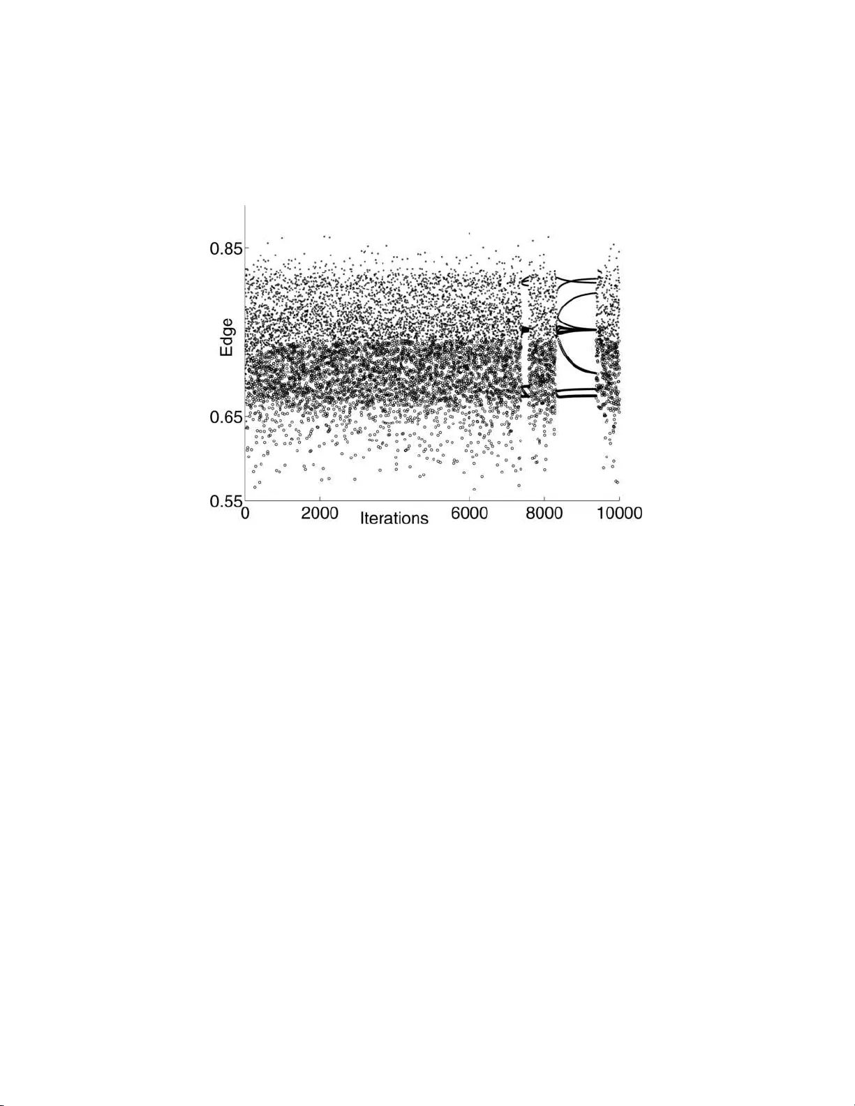
The Annals of Statistics 2007, V ol. 35, No. 6, 2723–27 68 DOI: 10.1214 /00905 3607000000785 c  Institute of Mathematical Statistics , 2007 ANAL YSIS OF BOOSTING ALGORITHMS USING THE SMOOTH MAR GIN FUNCTION By Cynthia R ud in 1 , 2 , 3 , R ob er t E. Schap ire 3 , 4 and Ingrid D aubechies 1 , 5 Columbia University, Princ eton Univ e rsity and Princ eton University W e introduce a useful tool for analyzing b oosting algorithms called the “smooth margin function,” a diﬀeren t iable appro x imation of the usual margi n for b o osting algorithms. W e present t wo bo osting algorithms based on this smooth margin, “co ordinate ascent b o ost- ing” and “approximate coordinate ascent b oosting,” whic h are simila r to F reund and Sc hapire’s AdaBo ost algorithm and Breiman’s arc-gv algorithm. W e give con vergence rates to the maximum margin solu- tion for b oth of our algorithms and for arc-gv. W e then study Ad- aBoost’s conv ergence prop erties using t he smo oth margin function. W e precisely b ound the margin attained by A daBoost when th e edges of the weak classiﬁers fall within a sp eciﬁed range. This show s that a previous b ound prov ed by R¨ atsc h and W armuth is exactly tigh t. F ur- thermore, we use the smo oth margin t o capture explicit prop erties of AdaBoost in cases where cyclic beh a vior occurs. 1. In trod uction. Bo osting algorithms, which construct a “strong” classi- ﬁer us in g only a training set and a “wea k” learning algorithm, are curren tly among the most p opular and most successful algorit hms for statistical learn- ing (see, e.g., Caru ana and Niculescu-Miz il’s recen t empirical comparison of Received Octob er 2004; rev ised March 2007. 1 Supp orted by NS F Grants DMS-98-10783 and DMS-02-19233 and Universit y of Wis- consin Gran t 640F161. 2 Supp orted by an NSF Postdoctoral Researc h F ello wship and a grant from the How ard Hughes Medical Institute. 3 Supp orted by NSF Grant I IS -03-25500. 4 Supp orted by NSF Grant CCR-03-25463. 5 Supp orted by AFOSR Gran t F49620 -01-1-0099. This w ork was done while CR’s aﬃliations were Program in A pplied and Computational Mathematics and Department of Computer Science, Princeton Univers ity; and Center for Neural Science and Courant Institute of Mathematical Sciences, New Y ork Universit y . AMS 2000 subje ct classiﬁc ations. Primary 68W40, 68Q25; secondary 68Q32. Key wor ds and phr ases. Boosting, AdaBo ost, large margin classiﬁcation, co ordinate de- scen t, arc-gv, con vergence rates. This is an electro nic reprint of the original a r ticle published b y the Institute of Mathematical Statistics in The Annals of Statistics , 2007, V ol. 35, No. 6, 2 723– 2768 . This repr int diﬀers from the original in pagination and t yp og raphic detail. 1 2 C. RUDIN, R. E. SCHAPIRE A ND I. DAUBEC HIES algorithms [ 3 ]). F reund and Sc hapire’s AdaBoost algorithm [ 7 ] w as the ﬁrst practical bo osting alg orithm. AdaBoost main tains a discret e distribution (set of w eight s) o v er the training examples, and sele cts a we ak cl assiﬁer via the w eak learning alg orithm at eac h iteration. T r aining examples that w ere misclassiﬁed b y the w eak classiﬁer at the curren t iteration then receiv e higher w eights at th e follo wing iteration. Th e end result is a ﬁnal com bined classiﬁer, giv en b y a thresholded linear combinat ion of the weak classiﬁers. See [ 13 , 27 ] f or an in tro d uction to b o osting. Shortly after AdaBoost was int ro duced, it w as observ ed th at AdaBoost often do es not seem to su ﬀer f r om o verﬁtting, in the sense that the test error do es not go u p eve n after a rather large n u m b er of iterations [ 1 , 5 , 14 ]. T his lac k of o v erﬁ tting wa s later explained b y Sc hapir e et al. [ 28 ] in terms of the mar gin the ory . The mar g i n of a b o osted classiﬁer on a particular example is a n umber b et ween − 1 and +1 that can b e in terpreted as a measure o f the classiﬁer’s conﬁdence on this particular example. F u rther, the minim u m margin ov er all examples in the training set is often referred to simp ly as the margin of the tra ining set , or simp ly the margin w hen clear from con text. Brieﬂy , the margin theory states that AdaBo ost tends to increase the mar- gins of the training examples, and that this increase in the margins imp lies b etter generalization p erformance. A complete analysis of AdaBo ost’s margin is n on trivial. Unt il recen tly , it w as an open question whether or not AdaBoost alw a ys ac hiev es the max- im u m p ossible margin. This question w as settled (negativ ely) in [ 20 , 22 ]; an example w as presen ted in w hic h AdaBo ost’s asymptotic margin w as pro ved to b e signiﬁcant ly b elo w the maxim um v alue. This example exhibited “cyclic ” b ehavior, where AdaBo ost’s parameter v alues rep eat p erio dically . So AdaBo ost d o es not generally maximize the margin; fu rthermore, unt il the present work, the cycl ic case was the only case for whic h AdaBo ost’s con ve rgence w as fully un d ersto o d in th e separable setting. When it cannot b e pr o ve d that the parameters will even tually settle do wn into a cycle, Ad- aBoost’s conv ergence prop erties are more diﬃcult to analyze. Y et it seems essen tial to understand this con verge nce in ord er to stu dy AdaBo ost’s gen- eralizat ion capabilities. In this w ork, we in tro du ce a n ew to ol f or analyzing AdaBoost and related algorithms. This to ol is a diﬀerenti able app r o ximation of the usual margin called the smo oth mar gin function . W e use it to provi de th e follo wing main con tributions. • W e id en tify an imp ortan t new setting for which AdaBo ost’s con v ergence can b e co mpletely understo o d , called the case of b ounde d e dges . A sp e- cial case of our pr o of sh o ws that th e margin boun d of R¨ atsc h and W ar- m u th [ 17 ] is tigh t, closing what they allude to as a “gap in theory .” This sp ecial case answ ers the question of how far b elo w maximal AdaBo ost’s BOOSTING AND THE SMOOTH MARGIN 3 margin can b e. F urth erm ore, this clariﬁes in sharp and precise terms the asymptotic relationship b et ween the “edge s” ac hiev ed by the weak learn- ing algorithm and the asymptotic margin of Ad aBoost. • W e deriv e t wo new algorithms similar to AdaBo ost that are based directly on the smo oth margin. Unlike AdaBo ost, these algorithms pro v ably con- v erge to a maximum margin solution asymptotically; in addition, they p ossess a fast con verge nce rate to a maxim u m margin solution. Simi- lar con verge nce rates based on the smo oth margin are then presen ted for Breiman’s arc-gv algorithm [ 2 ] answ ering what h ad b een p osed as an op en problem by Meir and R¨ atsc h [ 13 ]. 1.1. The c ase of b ounde d e dges. There is a ric h literature connecting AdaBoost and margins. The margin theory of Sc hapire et al. [ 28 ] (la ter tigh tened by Koltc h inskii and P anc henko [ 10 ]) sho wed th at the large r the margins on the training examples, the b etter an upp er b ound on the gener- alizat ion error, su ggesting that, all else b eing equal, the general ization error can b e reduced by systematica lly increasing the margi ns on the training set. F urthermore, Sc hapire et al. show ed that AdaBo ost has a tendency to increase the margins on the training examples. Thus, though not enti rely complete, their theory and exp erimen ts strongly s upp orted the notion th at margins are highly relev an t to the b eha vior and generalizat ion p erformance of AdaBo ost. These b ounds can b e reformulate d (in a slightl y w eak er form) in terms of the minimum margin; this w as the fo cus of p r evious work by Breiman [ 2 ], Gro ve and Sch uur mans [ 9 ] and R ¨ atsc h and W arm u th [ 17 ]. It is natural, giv en suc h an analysis, to pursue algorithms that will attempt to maximize this minim um margin. Suc h algorithms in cluded Breiman’s arc-gv algorithm [ 2 ] and Gro ve and Sch uur m ans’ LP-AdaBo ost [ 9 ] algorithm. How ev er, in appar- en t cont radiction of the margins theory , Breiman’s exp erimen ts indicated that his algorithm ac hieve d h igher margins than Ad aBoost, and y et p er- formed w orse on test data. Although this wo uld seem to indicate s erious trouble for the margins theory , recen tly , Reyzin and Sc hapire [ 18 ] revisited Breiman’s exp erimen ts and w ere able to reconcile his r esults with the mar- gins explanation, noting that the we ak classiﬁers found b y arc-gv are more complex than those found by AdaBo ost. When this complexit y is cont rolled, arc-gv con tinues to achiev e larger minim um margins, bu t AdaBoost ac hiev es m u c h higher margins o v erall (and generally b etter test p erformance). Y ears earlier, Grov e and Sc huurmans [ 9 ] observed the s ame phenomenon; highly con trolled exp erimen ts sho w ed that AdaBo ost ac hiev ed small er minim um margins, o verall larger margins, and often b etter test p erformance than LP- AdaBoost. T aken together, these results in dicate that there is a d elicate and complex balance b et w een the p erformance of the wea k learning algorit hm, the mar- gins, the problem d omain, the sp eciﬁc b o osting algorithm b eing used, and 4 C. RUDIN, R. E. SCHAPIRE A ND I. DAUBEC HIES Fig. 1. Plot of Υ( r ) ve rsus r (lower curve), along wi th the function f ( r ) = r (upp er curve). the test error. It is the goal of the curren t wo rk to improv e our und erstanding of the intricat e relationships b et we en th ese v arious facto rs. In considering these complex relatio nships, a piece of the puzzle ma y b e determined theoretically b y understanding AdaBoost’s con ve rgence. Ad- aBoost h as b een shown to ac hiev e large margins, but not maximal margins. T o b e precise, Schapire et al. [ 28 ] sho wed that AdaBo ost ac hieve s at least half of the maxim um margin, that is, if the maxim um margin is ρ > 0, AdaBo ost will ac hiev e a margin of at least ρ/ 2. This b ound w as tigh tened by R¨ atsc h and W armuth [ 17 ] who sho wed that AdaBo ost asymptotically ac h iev es a margin of at least Υ( ρ ) > ρ/ 2, where Υ : (0 , 1) → (0 , ∞ ) is the mon otonically increasing fun ction sho wn in Figure 1 , namely , Υ( r ) := − ln( 1 − r 2 ) ln((1 + r ) / (1 − r )) . (1.1) Ho wev er there is still a large gap b et ween Υ( ρ ) a nd the maxim um margin ρ . Our con tribu tion is from the other d irection; w e ha v e just describ ed theo- retical lo w er b ounds for the m argin, whereas w e are now in terested in upp er b ound s. Previously , w e sh ow ed that it is p ossible for AdaBo ost to ac hiev e a margin that is signiﬁcan tly b elo w the maximal v alue [ 22 ]. In this w ork, we sho w that R¨ atsc h and W armuth’s b oun d is ac tually tigh t. In other words, w e prov e that it is p ossible for AdaBo ost to achie v e an asymptotic m argin arbitrarily close to Υ( ρ ). More generally , our theorem regarding the case of “b ounded edges” sa ys the follo w ing, wh ere the “edge ” measures the p erfor- mance of the w eak learning algorit hm at eac h iterati on: • If AdaBo ost’s edge v alues are within a range [ ¯ ρ, ¯ ρ + σ ] for some ¯ ρ ≥ ρ , then AdaBoost’s margin asymptotica lly lies within the in terv al [Υ( ¯ ρ ) , Υ( ¯ ρ + σ )]. BOOSTING AND THE SMOOTH MARGIN 5 Hence there is a fundamen tal connecti on b et wee n the p erformance of the w eak learning algorithm an d AdaBo ost’s asymptotic margin; if AdaBo ost’s edges fall within a gi v en in terv al, w e ca n ﬁnd a corresp onding int erv al for its asymptotic margin. No w, since w e ha ve pr o ve n that we can more or less p redetermine the v alue of AdaBo ost’s margin simp ly b y s p ecifying the edge v alues, w e can p erform a new exp eriment. Since the studies of Breiman [ 2 ] and Gro v e and Sc huurmans [ 9 ] suggest that the margin th eory cannot b e easily tested u sing m u ltiple algorithms, we no w p erform a con trolled study with only one algo- rithm. The exp erimen t in S ection 7.2 consists of man y trials w ith the s ame algorithm (AdaBo ost) ac hieving diﬀerent v alues of the margin on the same dataset. W e ﬁnd that as the (predetermined) margin increases, the pr oba- bilit y of error on test data d ecreases dramatical ly . O ur exp eriment supp orts the margin theory; in at least some cases, a larger margin d o es correlate with b etter generalizat ion. 1.2. Conver ge nc e pr op erties of new and old algorithm s. Since Ad aBoost ma y ac hiev e a margin as lo w as Υ( ρ ), and since it has the idiosyncratic (alb eit fascinat ing and p ossibly helpful) tendency to sometimes get stuc k in cyclic patterns [ 11 , 22 , 23 ], we are inspired to ﬁn d algorithms that are similar to Ad aBoost that h a ve b etter con ve rgence guaran tees. W e also stu d y these cyclic patterns of Ad aBoost as a sp ecial case for understandin g its general con ve rgence prop erties. Our ﬁrst main fo cus is to analyze t w o algorithms d esigned to maximize the smo oth m argin, calle d co ordinate ascen t b o osting and appro ximate co ordi- nate ascen t b o osting (presente d in our previous w ork [ 23 ] without analysis). Co ordinate ascen t/descen t algorithms are optimization algorithms w here a step is made along only one coordinate at ea c h iteration. The c o ordinate, whic h is also the choi ce of weak classiﬁer, is determined by the wea k learning algorithm. AdaBoost is also a co ordinate descent algorithm [ 2 , 6 , 8 , 12 , 16 ], but its ob jectiv e function need not b e d irectly rela ted to the margin or smo oth margin; in fact, Ad aBoost’s ob jectiv e con v erges to zero whenev er the asymptotic margin is any p ositiv e v alue. There are other algorithms designed to maximize the margin, though not based on co ordinate ascent /descen t of a ﬁxed ob jectiv e f unction. Here is a description of the known con verge nce prop erties of the r elev ant algo rithms: AdaBoost do es not con verge to a maxim u m margin solution. Breiman’s arc- gv algorithm [ 2 , 13 ] h as b een pro v en to conv erge to the maximum m argin asymptoticall y , but we are not a w are of an y pr o ven con vergenc e rate prior to this work. (N ote that Meir and R¨ atsc h [ 13 ] giv e a v ery simple asymp- totic con v ergence pro of for a v arian t of arc-gv; ho wev er, they note that n o con ve rgence rate can b e d erived fr om the p r o of.) R¨ atsc h and W armuth’s AdaBoost ∗ algorithm [ 17 ] has a fast con verge nce rate, namely , it yields a 6 C. RUDIN, R. E. SCHAPIRE A ND I. DAUBEC HIES solution within ¯ ν of the maxim um margin in 2(log 2 m ) / ¯ ν 2 steps, where m is the num b er of training examples. Ho w ever, the “greediness” p arameter ¯ ν must b e manual ly entered (and p erhaps adju sted) by the user; the algo- rithm is quite sensitiv e to ¯ ν . If it is estimated sligh tly to o large or to o small, the algorithm either tak es a long time to conv erge, or it will not ac hiev e the d esired precision. (E.g., th e exp eriment s in [ 17 ] sho w that the algorithm p erforms we ll only for ¯ ν in a carefully c hosen range. In [ 25 ], ¯ ν w as estimate d sligh tly too small, and the algorithm did not con verge in a timely manner.) F or any ﬁ xed v alue of ¯ ν , asymptotic con ve rgence is not guaran teed and will generally not b e ac hieve d. In con trast to previous algorithms, the ones we in tro duce ha ve a p ro ven fast conv ergence rate to the maxim u m margin, they h a ve asymptotic con- v ergence to the maxim um margin, they do not require a c hoice of greediness parameter since the greediness is adaptiv ely adju sted b ased on the progress of th e algorithm, and they are based on co ordinate ascen t of a sens ib le ob jec- tiv e, namely th e smo oth m argin. The conv ergence r ates for our algorithms and for arc-gv are custom-designed using recursiv e equaliti es for the smo oth margin; we kno w of n o standard tec h niques that would allo w us to obtain suc h tigh t rates. W e also fo cus on the con v ergence prop erties of Ad aBoost itself, u s ing the smo oth margin as a helpful analytical to ol. T he usefulness of the smo oth margin f ollo ws largely from an imp ortan t theorem, wh ic h sho ws that the v alue of the smo oth margin increases if and only if AdaBo ost tak es a “large enough” step. Muc h previous w ork has fo cused on the statistical p rop erties of AdaBo ost indir ectly through generaliza tion b ounds [ 10 , 28 ], whereas our goal is to explore the wa y in whic h AdaBo ost actual ly con verge s in order to pro du ce a p o werful classiﬁer. In S ection 7.1 , we use the smo oth margin function to pro ve general prop- erties of AdaBo ost in cases where cyclic b ehavio r occur s , extending pr evious w ork [ 22 , 23 ]. “Cyclic b eh avio r for Ad aBo ost” means that the weak learn- ing algorithm rep eatedly c h o oses the same sequence of w eak classiﬁers, and the we igh t v ectors rep eat with a give n p erio d. When the num b er of train- ing examples is sm all, it is lik ely that this b eha vior will b e observ ed. Ou r ﬁrst main result concerning cyclic AdaB o ost is a pro of that the v alue of the smo oth margin must decrease an inﬁn ite num b er of times m o dulo one exception. Th u s , a p ositiv e qualit y whic h holds for our new algorit hms do es not hold for Ad aBoost: our new algorithms alw ays increase the smo oth mar- gin at ev ery iteration, whereas cyclic AdaBo ost usu ally cannot. The single exception is the case wh ere all edge v alues are identica l. Our second result in this s ection concerns this exceptional case. W e show that if all edges in a cycle are identi cal, then all supp ort v ectors (examples nearest the decision b ound ary) are m isclassiﬁed b y the same num b er of w eak classiﬁers d uring the cycle. Thus, in this exceptio nal case, a strong equiv alence exists b etw een BOOSTING AND THE SMOOTH MARGIN 7 supp ort v ectors; they are misclassiﬁed the same prop ortion of the time by the weak learning algorithm. Here is the outline for the full pap er. In Section 2 , w e int ro duce our no- tation and explain the AdaBo ost algo rithm. In S ection 3 , w e d escrib e t he smo oth ma rgin fu n ction that o ur a lgorithms a re base d on. In Section 4 , w e d escrib e co ordin ate ascen t b o osting (Algorithm 1) and appro ximate co- ordinate ascen t b o osting (Algorithm 2), and in Section 5 , the conv ergence of these a lgorithms is discussed, alo ng with th e con verge nce of arc-gv in Section 6 . In Section 7 , we show connections b et wee n AdaBoost and our smo oth margin fu nction. Sp eciﬁcally , in Section 7.1 , w e fo cus on cyclic Ad- aBoost, and in Section 7.2 , w e discuss the case of b ounded edges, including the exp eriment describ ed earlier. S ections 8 , 9 and 10 conta in proofs fr om Sections 3 , 5 , 6 and 7 . Preliminary and less deta iled statemen ts of these results app ear in [ 25 , 26 ]. 2. Notatio n and introduction to AdaBo ost. Our nota tion is similar to that of Collins, Sc h apire and Singer [ 4 ]. T he training set consists of examples with lab els { ( x i , y i ) } i =1 ,...,m , m > 1, where ( x i , y i ) ∈ X × {− 1 , 1 } . The space X neve r app ears explicitly in our calcula tions. Let H = { h 1 , . . . , h n } b e the set of all p ossible wea k classiﬁers that can b e pro du ced by the weak learning algorithm, where h j : X → {− 1 , 1 } . (The h j ’s are not assumed to b e linearly indep end ent; it is ev en p ossible that b oth h and − h b elong to H .) Sin ce our classiﬁers are binary , and since we restrict our atten tion to their b ehavio r on a ﬁnite training set, we can assume the n um b er of weak classiﬁers n is ﬁ nite. W e typica lly think of n a s b eing large, m ≪ n , w hic h mak es a gradien t d escen t calculation impractica l; wh en n is not large, the linear program can b e solv ed d ir ectly using an algorithm suc h as LP-AdaBo ost [ 9 ]. The classiﬁcatio n rule that AdaBo ost outputs is f Ada , λ where sign( f Ada , λ ) indicates the predicted class. T he form of f Ada , λ is f Ada , λ := P n j =1 λ j h j k λ k 1 , where λ ∈ R n + is the (unnormalized) co eﬃcient v ector. W e deﬁne the 1-norm k λ k 1 as usual: k λ k 1 := P n j =1 λ j . A t iteration t of Ad aBo ost, the co eﬃcien t v ector is λ t , and the sum is denoted s t := k λ t k 1 . W e deﬁn e an m × n matrix M where M ij = y i h j ( x i ), that is, M ij = +1 if training example i is classiﬁed correct ly by w eak classiﬁer h j , and − 1 other- wise. W e assume that no column of M h as all + 1’s, that is, no wea k classi- ﬁer can classify all the training examples correctly . (Otherwise the learning problem is trivial.) This n otatio n is useful m athematica lly for our analysis; ho wev er, it is not generally wise to explicitly construct large M in practice since the w eak learning alg orithm pro vides the necessary co lumn for eac h 8 C. RUDIN, R. E. SCHAPIRE A ND I. DAUBEC HIES iteratio n. M acts as the only “input” to AdaBo ost in this notation, con tain- ing all the necessary information ab out the w eak learning algorit hm and training examples. The margin theory dev elop ed via a set of generalizat ion b ounds that are based on the m argin distribution o f the training exa mples [ 10 , 28 ], where the mar gin of tr aining example i with resp ect to classiﬁer λ is deﬁned to b e y i f Ada , λ ( x i ), or equiv alen tly , ( M λ ) i / k λ k 1 . These b ounds can b e reformu- lated (in a sligh tly w eak er form) in terms of the minimum margin. W e call the minimum margin o ver the training examples the mar gin of the training set, denoted µ ( λ ), that is, µ ( λ ) := min i ( M λ ) i k λ k 1 . An y training example i w hose margin is equal to the minim um margin µ ( λ ) will b e called a supp ort ve c tor . (Th ere is a tec hn ical remark ab out our def- inition of AdaBo ost. A t iteration t , the (unnorm alized) co eﬃcien t v ector is denoted λ t ; i.e., the co eﬃcient of w eak classiﬁer h j determined b y Ad- aBoost at iteration t is λ t,j . In the n ext iteration, all but one of the en tries of λ t +1 are the same as in λ t ; the only en try that is c hanged (for index j = j t ) is giv en a p ositiv e increment in our description of AdaBo ost, i.e., λ t +1 ,j t > λ t,j t . S tarting from λ 1 = 0 , this means that all the λ t for t > 1 ha ve nonn egativ e e n tries. W e thus need to study the eﬀect of AdaBo ost only on the positive cone R n + := { λ ∈ R n ; ∀ j λ j ≥ 0 } . This same formali za- tion w as imp licitly used in e arlier w orks [ 17 , 28 ]. Note that there are also formalizatio ns; e.g., see [ 19 ], where entries of λ are p ermitted to decrease . The presen t formula tion is also charact erized by its fo cus on the co eﬃcien t v ector λ as the “fun d amen tal ob j ect,” as opp osed to the functional P j λ j h j deﬁned b y taking the λ j as we igh ts fo r the h j . This is expressed b y our c hoice of the ℓ 1 norm: k λ k 1 = P j | λ j | to “measure” λ ; if one f o cuses on the functional instea d, then it is n ecessary to tak e into accoun t that (b ecause of the p ossible linear dep endence of the h j ) sev eral diﬀerent c hoices of λ can giv e rise to th e same f unctional. (E.g., if for some pair ℓ, ℓ ′ w e ha v e h ℓ ′ = − h ℓ , then adding α to b oth λ ℓ and λ ℓ ′ do es not c hange P j λ j h j .) On e m u st then use a norm that “quotien ts o ut” this am b iguit y , as in (for in- stance) k | λ k | := min {k a k 1 ; P j a j h j = λ j h j } . By restricting ours elv es to p osi- tiv e incremen ts only , and using the ℓ 1 -norm of λ t , w e a v oid those non unique issues. F or our n ew algorithms, we p ro ve lim t →∞ [min i ( M λ t ) i / k λ t k 1 ] = ρ , and where ρ is the maxim um p ossible v alue of this quan tit y (deﬁn ed later). Since k λ t k 1 ≥ k | λ t k | , and ρ i s an upp er b ound for these f r actions, it fol- lo ws automatically that for our algo rithms, lim t →∞ [min i ( M λ t ) i / k | λ k | ] = ρ as well; i.e., we prov e conv ergence to a maxim u m margin solution eve n for the fu nctional b ased norm. AdaBo ost itself cannot b e guaran teed to reac h BOOSTING AND THE SMOOTH MARGIN 9 the maxim u m margin solution in the limit, regardless of whether k λ t k 1 or k | λ t k | is used in the denominator.) A b o osting algorithm main tains a distribution, or set of wei gh ts, o v er the training examples that is up dated at eac h iteration t . This distribu tion is denoted d t ∈ ∆ m , and d T t is its transp ose. Here, ∆ m denotes the sim- plex of m -dimensional vec tors with nonnegat iv e en tries that sum to 1. A t eac h iteration t , a w eak classiﬁer h j t is selecte d by the w eak learning algo- rithm. The probabilit y of error at iterati on t , denoted d − , of the select ed w eak classiﬁer h j t on the training examples (w eigh ted by the d iscrete dis- tribution d t ) is d − := P { i : M ij t = − 1 } d t,i . Also, denote d + := 1 − d − . Deﬁne I + := { i : M ij t = +1 } , the set of correctly classiﬁed examples at iteration t , and similarly deﬁne I − := { i : M ij t = − 1 } . Note that d + , d − , I + , and I − de- p end on t ; although w e ha v e simpliﬁed the n otatio n, t he iteration num b er will b e clear from the con text. The e dge of weak classiﬁer j t at time t is r t := ( d T t M ) j t = d + − d − = 1 − 2 d − , with ( · ) k indicating th e k th v ector comp onent . Th u s, a larger edge indicates a lo wer probability of error. Note that d + = (1 + r t ) / 2 and d − = (1 − r t ) / 2. Also deﬁne γ t := tanh − 1 r t = 1 2 ln  1 + r t 1 − r t  . Due to the vo n Neumann Min–Max theorem for 2-pla yer zero-sum games, min d ∈ ∆ m max j ( d T M ) j = max ¯ λ ∈ ∆ n min i ( M ¯ λ ) i . That is, the minimum v alue of the maxim um edge (left-hand side) corre- sp onds to the maximum v alue of the margin. W e denote this v alue b y ρ . W e w ish our learning algo rithms to hav e robus t con ve rgence, so w e will n ot generally r equ ir e the w eak learning algorithm to pro du ce the wea k classiﬁer with the largest p ossible edge v alue at eac h iterati on. Rather, we only require a w eak classiﬁer wh ose edge exceeds ρ , that is, j t ∈ { j : ( d T t M ) j ≥ ρ } . This notion of robustness has b een previously used for the analysis of AdaBo ost ∗ and arc-gv. Here, AdaBoost in the optimal case means that the b est w eak classiﬁer is c hosen at eve ry iterat ion: j t ∈ arg max j ( d T t M ) j , while AdaBoost in the nonoptima l case means that an y go o d enough weak classiﬁer is c hosen: j t ∈ { j : ( d T t M ) j ≥ ρ } . The case of b ounde d e dges is a subset of the n onopti- mal case for some ¯ ρ ≥ ρ and σ ≥ 0 , namely j t ∈ { j : ¯ ρ ≤ ( d T t M ) j ≤ ¯ ρ + σ } . W e are in terested in the sep ar able ca se w here ρ > 0 and the training error is zero; the margin sp eciﬁcally allo ws us to distinguish b et ween classiﬁers that ha ve zero training error. In the n onseparable case, AdaBoost’s ob jectiv e function F is an upp er b ound on the training error, and conv ergence is w ell understo o d [ 4 ]. Not only do es AdaBo ost con verge to the minimum of F , but it has recen tly b een sho w n that it conv erges to the solution of the “bipartite 10 C. RUDIN, R. E. SCHAPIRE A ND I. DAUBEC HIES 1. Input: Matrix M , No. of iterations t max 2. Initialize: λ 1 ,j = 0 for j = 1 , . . . , n , also d 1 ,i = 1 /m for i = 1 , . . . , m , and s 1 = 0 . 3. Lo op for t = 1 , . . . , t max (a)  j t ∈ argmax j ( d T t M ) j optimal case j t ∈ { j : ( d T t M ) j ≥ ρ } nonoptimal case  (b) r t = ( d T t M ) j t (c) g t = max[0 , G ( λ t )] where G ( λ t ) is deﬁned in ( 3.1 ), G ( λ t ) = ( − ln P m i =1 e − ( M λ t ) i ) /s t . (d)                  α t = 1 2 ln  1 + r t 1 − r t  AdaBoost α t = 1 2 ln  1 + r t 1 − r t  − 1 2 ln  1 + g t 1 − g t  appro x co ord ascent b o osting If g t > 0 , α t = argmax α G ( λ t + α e j t ) , co ord ascen t b o osting else use AdaBo ost.                  (e) λ t +1 = λ t + α t e j t , wh ere e j t is 1 in p osition j t and 0 elsewhere. (f ) s t +1 = s t + α t (g) d t +1 ,i = d t,i e − M ij t α t /z t where z t = P m i =1 d t,i e − M ij t α t 4. Output: λ t max /s t max Fig. 2. Pseudo c o de for the A daBo ost algorithm, c o or dinate asc ent b o osting and appr oxi- mate c o or dinate asc ent b o osting. ranking problem” at the same time; Ad aBoost solv es t wo problems for the price of one in the nons eparable case [ 21 , 24 ]. Ho wev er, in th e separable case, where F cannot distinguish b etw een classiﬁers since it simp ly con ve rges to zero, the margin theo ry suggests that we not only m inimize F , but also distinguish b etw een classiﬁers by c h o osing one that maximizes the margin. Since one do es not know in adv ance whether the problem is separable, in this work we use AdaBoost u n til the problem b ecomes separable, and then p erhaps switch to a mo de designed explicitly to maximize the margin. Figure 2 shows the ps eu d o co de for AdaBoost, co ordinate ascen t b o osting, and appr o ximate co ordinate ascen t b o osting. O n eac h roun d of b o osting, classiﬁer j t with suﬃcien tly large edge is select ed (Step 3a), the w eigh t of that classiﬁer is up dated (Step 3e), and the distribution d t is up d ated and renormalized (Step 3g). Note that λ t,j = P t ˜ t =1 α ˜ t 1 j ˜ t = j , where 1 j ˜ t = j is 1 if j ˜ t = j and 0 otherwise. The notation e j t means the v ector that is 1 in p osition j t and 0 elsewhere. 2.1. A daBo ost is c o or dinate desc e nt. AdaBo ost is a coordinate descen t algorithm for minimizing F ( λ ) := P m i =1 e − ( M λ ) i . This has b een sh o wn m an y times [ 2 , 6 , 8 , 12 , 16 ], so w e will only sket c h the pro of to in tro duce our BOOSTING AND THE SMOOTH MARGIN 11 notation. Th e dir ection AdaBo ost chooses at iteration t (corresp onding to the choi ce of we ak classiﬁer j t ) in the optimal case is j t ∈ arg max j  − dF ( λ t + α e j ) dα    α =0  = arg m ax j m X i =1 e − ( M λ t ) i M ij = arg m ax j ( d T t M ) j . The step size AdaBo ost c ho oses a t iteration t is α t , where α t satisﬁes the follo wing equation, that is, the equation f or the line searc h along direction j t : 0 = − dF ( λ t + α t e j t ) dα t = m X i =1 e − ( M ( λ t + α t e j t )) i M ij t , 0 = d + e − α t − d − e α t , α t = 1 2 ln  d + d −  = 1 2 ln  1 + r t 1 − r t  = tanh − 1 r t = γ t . Note that for b oth the optimal and nonoptimal cases, α t ≥ tanh − 1 ρ > 0, b y monotonicit y of tanh − 1 . In the nonseparable ca se, the d t ’s conv erge to a ﬁxed vec tor [ 4 ]. I n the separable case, the d t ’s cannot con verge to a ﬁxed ve ctor, and the minimum v alue of F is 0, o ccurrin g as k λ k 1 → ∞ . It is imp ortant to appreciate that this tells us nothing a b out the v alue of the margi n ac h iev ed b y AdaBoost or any other pr o cedure designed to minimize F . In fact, an arb itrary algo- rithm that minimizes F can ac hieve an arbitrarily bad (small) margin. [T o see wh y , consider an y ¯ λ ∈ ∆ n suc h that ( M ¯ λ ) i > 0 for all i , assuming w e are in the separable case so such a ¯ λ exists. Then lim a →∞ a ¯ λ w ill pr o duce a minim um v alue f or F , b ut the original normalized ¯ λ n eed not yield a max- im u m margin.] So it m us t b e the pr o c ess of coordin ate descen t that aw ards AdaBoost it s abilit y to increase m argins, not simply AdaBo ost’s abilit y to minimize F . The v alue of the fun ction F tel ls us ve ry little ab out the v alue of the margin; e v en asymp totica lly , it only tell s us whether the margin is p ositiv e or n ot. A helpful prop erty of AdaBo ost is that we can do the line searc h at eac h step explicitly; that is, w e hav e an analytica l expr ession for the v alue of α t for eac h t . Our second b o osting algorithm, appro ximate coordinate asce n t b o osting, whic h incorp orates an appr o ximate line searc h, also h as an up date that can b e solv ed explicitly . 3. The s mo oth margin function G ( λ ) . W e wish to consid er a fun ction that, u nlik e F , actually tells us ab out the v alue of the margin. Our n ew function G has the nice prop ert y that its maxim um v alue corresp onds to 12 C. RUDIN, R. E. SCHAPIRE A ND I. DAUBEC HIES the maximum v alue of the margin. Here, G is deﬁned for λ ∈ R n + , k λ k 1 > 0 b y G ( λ ) := − ln F ( λ ) k λ k 1 = − ln( P m i =1 e − ( M λ ) i ) P j λ j . (3.1) One can think of G as a smo oth approxi mation of the margin, since it dep ends on the en tire margin distribution when k λ k 1 is small, and w eigh ts training examples with small margins m uch more highly than examples with larger margins, esp ecially as k λ k 1 gro ws. The fu nction G also b ears a re- sem b lance to the ob jectiv e implicitly u s ed for ε -b o osting [ 19 ]. G has man y nice prop erties that are useful for un d erstanding its geometry: Pr oposition 3.1 (Prop erties of the smo oth margin [ 25 ]). 1. G ( λ ) is a c onc ave function (bu t not ne c e ssarily strictly c onc ave) in e ach “ shel l ” wher e k λ k 1 is ﬁxe d. 2. The value of G ( λ ) incr e ases r adial ly, that is, G ( a λ ) > G ( λ ) for a > 1 . 3. As k λ k 1 b e c omes lar ge, G ( λ ) tends to µ ( λ ) . Sp e ciﬁc al ly, − ln m k λ k 1 + µ ( λ ) ≤ G ( λ ) < µ ( λ ) . Pr oof. It follo ws from p rop erties 2 and 3 th at the m aximum v alue of G is the maximum v alue of the margin. The pr o ofs of prop erties 1 and 2 are in Section 8 . Od d ly enough, a la c k of conca vit y does n ot aﬀect our analysis, as our algorithms will iterativ ely maximize G , w hether or not it is conca v e. F or the pro of of prop ert y 3, me − µ ( λ ) k λ k 1 = m X i =1 e − min ℓ ( M λ ) ℓ ≥ m X i =1 e − ( M λ ) i > e − min i ( M λ ) i = e − µ ( λ ) k λ k 1 , and taking logarithms, dividin g b y k λ k 1 and negating yields the resu lt.  Since all v alues of the edge (ev en in the nonoptimal case) are required to b e larger than the maxim um margin ρ , w e ha ve for eac h iteratio n t , where recall s t := k λ t k 1 , − ln m s t + µ ( λ t ) ≤ G ( λ t ) < µ ( λ t ) ≤ ρ ≤ r t . (3.2 ) BOOSTING AND THE SMOOTH MARGIN 13 4. Deriv ation of algorithms. W e n ow suggest t w o b o osting algorithms that aim to maximize the margin explicitly (lik e arc-gv and AdaBoost ∗ ), are based on coordinate a scen t and adaptiv ely adjust their step sizes (like AdaBoost). Before w e deriv e the algo rithms, w e will write recursiv e equa- tions for F an d G . This will p ro vide a m etho d for computing th e v alues of F and G at iteratio n t + 1 in terms of th eir v alues at iteration t . The recursive equation for F is F ( λ t + α e j t ) = m X i =1 e − ( M ( λ t + α e j t )) i = X i ∈I + e − ( M λ t ) i e − α + X i ∈I − e − ( M λ t ) i e α = [ d + e − α + d − e α ] F ( λ t ) =  1 + r t 2 e − α + 1 − r t 2 e α  F ( λ t ) = [cosh α − r t sinh α ] F ( λ t ) . Here w e remind the reader that cosh x = ( e x + e − x ) / 2, sinh x = ( e x − e − x ) / 2, and so cosh(ta nh − 1 x ) = (1 − x 2 ) − 1 / 2 . Recall the deﬁnition γ t := tanh − 1 r t . Con tinuing to r educe, we ﬁ nd the recursiv e equation for F , F ( λ t + α e j t ) = cosh γ t cosh α − sinh γ t sinh α cosh γ t F ( λ t ) (4.1) = cosh( γ t − α ) cosh γ t F ( λ t ) . Here w e hav e used the iden tit y cosh( x − y ) = cosh x cosh y − sinh x sinh y . No w w e ﬁ n d a recursiv e equation for G . By deﬁnition of G , w e know − ln F ( λ t ) = s t G ( λ t ) . T aking the logarithm of ( 4.1 ) and negating, ( s t + α ) G ( λ t + α e j t ) = − ln F ( λ t + α e j t ) = − ln F ( λ t ) − ln  cosh( γ t − α ) cosh γ t  (4.2) = s t G ( λ t ) + ln  cosh γ t cosh( γ t − α )  = s t G ( λ t ) + Z γ t γ t − α tanh u du. Th us, w e ha v e a recursive equation for G . W e will deriv e t wo algorithms; in the ﬁ r st, we assign to α t the v alue α that maximizes G ( λ t + α e j t ), whic h requires sol ving an implicit equation. In the seco nd a lgorithm, w e pic k an appro ximate v alue for the maximize r that can b e computed in a straigh t- forw ard w a y . In b oth cases, since it is not kno wn in adv ance whether the problem is separable, the algo rithm starts by run ning AdaBoost until G ( λ ) 14 C. RUDIN, R. E. SCHAPIRE A ND I. DAUBEC HIES b ecomes p ositiv e, whic h ev en tually m ust happ en (in the separable case) b y the follo w ing: Pr oposition 4.1. In the sep ar able c ase (wher e ρ > 0 ), A daBo ost achieves a p ositive value for G ( λ t ) for some iter ation t . Pr oof. F or the iteration deﬁn ed by AdaBo ost (i.e., α t = γ t = tanh − 1 r t ), w e ha v e from ( 4.1 ) F ( λ t +1 ) = F ( λ t + γ t e j t ) = 1 cosh γ t F ( λ t ) = (1 − r 2 t ) 1 / 2 F ( λ t ) ≤ (1 − ρ 2 ) 1 / 2 F ( λ t ) . Hence, b y this recursion, F ( λ t +1 ) ≤ (1 − ρ 2 ) t/ 2 F ( λ 1 ). It follo ws that exceed- ing at most 2 ln F ( λ 1 ) − ln( 1 − ρ 2 ) + 1 iteratio ns, F ( λ t ) < 1 so that G ( λ t ) = ( − ln F ( λ t )) /s t > 0 .  F or con v enience in distinguishin g the t wo al gorithms deﬁned b elo w, we denote λ [1] 1 , . . . , λ [1] t to b e a sequence of co eﬃcien t v ectors generated by Algorithm 1, a nd λ [2] 1 , . . . , λ [2] t to b e a sequence generated b y Algorithm 2. Similarly , we d istinguish the sequences α [1] t from α [2] t , g [1] t := G ( λ [1] t ), g [2] t := G ( λ [2] t ), s [1] t := P j λ [1] t,j and s [2] t := P j λ [2] t,j . Sometimes w e compare the b eha vior of Algorithms 1 and 2 based on one iterat ion (from t to t + 1) as if they h ad started fr om the same co eﬃcient v ector at iteration t ; we d enote this vect or b y λ t . When an equation holds for b oth Algorithm 1 and Algo- rithm 2, we will often drop the sup erscripts. Although sequences su c h as j t , r t , γ t , and d t are also diﬀeren t for Algorithms 1 and 2, we lea ve the notation without the s up erscript. Note that it is imp ortan t to compute g t in a n umerically stable wa y . The pseudo co de in Figure 2 migh t th us b e replaced w ith G ( λ t ) = µ ( λ t ) − ln P m i =1 e − [( M λ t ) i − min i ′ ( M λ ) i ′ ] s t , where µ ( λ t ) = min i ( M λ t ) i s t . 4.1. Algorit hm 1: c o or dinate asc ent b o osting. Let us consider co ordinate ascen t on G . In what follo ws, w e will use only p ositiv e v alues of G , as w e BOOSTING AND THE SMOOTH MARGIN 15 ha ve justiﬁed via Proposition 4. 1 . The c h oice of direction j t at it eration t (in the optimal case) ob eys j t ∈ arg max j dG ( λ [1] t + α e j ) dα    α =0 = arg max j  P m i =1 e − ( M λ [1] t ) i M ij F ( λ [1] t )  1 s [1] t + ln( F ( λ [1] t )) ( s [1] t ) 2 . Of the t wo terms on the right, the second term do es not dep end on j , and the ﬁrst term is simply a constan t times ( d T t M ) j . Th us the same d irection will b e c h osen h ere as for AdaBoost. The “nonoptimal ” setting w e deﬁne for this alg orithm wil l b e the s ame as Ad aBo ost’s, so the weak learning algorithm (Step 3a) of Algorithm 1 will b e the same as AdaBo ost’s. T o determine the step size, ideally w e w ould lik e to maximize G ( λ [1] t + α e j t ) with resp ect to α , th at is, w e wo uld like to deﬁne the step size α [1] t to ob ey dG ( λ [1] t + α e j t ) /dα = 0 for α = α [1] t . Diﬀeren tiating ( 4.2 ) giv es ( s [1] t + α ) dG ( λ [1] t + α e j t ) dα + G ( λ [1] t + α e j t ) = tanh( γ t − α ) . Th us, our ideal step size α [1] t satisﬁes G ( λ [1] t +1 ) = G ( λ [1] t + α [1] t e j t ) = tanh( γ t − α [1] t ) . (4.3) There is not a nice analytica l solution f or α [1] t (as there is for AdaBo ost), but minimization of G ( λ [1] t + α e j t ) is one-dimensional so it can b e p erformed reasonably quickly . Hence we h a ve deﬁned the ﬁrst of our n ew b o osting algo- rithms, co ordinate ascen t on G , implement ing a line searc h at eac h iteratio n. F urth ermore: Pr oposition 4.2. The solution for α [1] t is unique, for some α [1] t > 0 . Pr oof. First, we rewrite the line searc h equation ( 4.3 ) using ( 4.2 ), s [1] t G ( λ [1] t ) + ln  cosh γ t cosh( γ t − α [1] t )  = ( s [1] t + α [1] t ) tanh ( γ t − α [1] t ) . Consider the f u nction f t , f t ( α ) := s [1] t G ( λ [1] t ) + ln  cosh γ t cosh( γ t − α )  − ( s [1] t + α ) tanh( γ t − α ) . No w, d f t ( α ) /dα = ( α + s [1] t )sec h 2 ( γ t − α ) > 0 for α > 0 . Thus f t is strictly increasing, so there is at most one ro ot. W e also h a ve f t (0) = s [1] t ( G ( λ [1] t ) − 16 C. RUDIN, R. E. SCHAPIRE A ND I. DAUBEC HIES r t ) < 0 and f t ( γ t ) = s [1] t G ( λ [1] t ) − 1 2 ln(1 − r 2 t ) > 0. Th us, b y the in termediate v alue theorem, there is at least one ro ot. Hence, there is exactly one solution for α [1] t where α [1] t > 0 .  Let us rearrange our equations sligh tly in order to study the up date. Using the notation g [1] t +1 := G ( λ [1] t +1 ) in ( 4.3 ), we ﬁ nd that α [1] t satisﬁes the follo win g (implicitly): α [1] t = γ t − tanh − 1 ( g [1] t +1 ) = tanh − 1 r t − tanh − 1 ( g [1] t +1 ) (4.4) = 1 2 ln  1 + r t 1 − r t 1 − g [1] t +1 1 + g [1] t +1  . Since G ( λ [1] t +1 ) ≥ G ( λ [1] t ), we again ha v e G ( λ [1] t +1 ) > 0, and th us α [1] t ≤ tanh r t = γ t . Hence, the step size f or th is n ew algorithm is alw ays p ositiv e, and it is upp er-b ounded b y AdaBoost’s step size. 4.2. Algorit hm 2: a ppr oximate c o or dinate asc ent b o osting. Th e second of our tw o n ew b o osting algorithms a v oids the line searc h of Algorithm 1, and is ev en slig h tly more aggressiv e. It seems to perf orm ve ry similarly to Algorithm 1 in our exp erimen ts. T o deﬁne this algorithm, we consider the follo wing app r o ximate solution to the maximization problem, b y using an appro ximate solution to ( 4.3 ) at eac h iteration in whic h λ t +1 is replaced by λ t for tractabilit y: G ( λ [2] t ) = tanh( γ t − α [2] t ) , (4.5) or more explicitl y , α [2] t = γ t − tanh − 1 ( g [2] t ) = tanh − 1 r t − tanh − 1 ( g [2] t ) (4.6) = 1 2 ln  1 + r t 1 − r t 1 − g [2] t 1 + g [2] t  . The up date α [2] t is also strictly p ositiv e, since g [2] t < ρ ≤ r t , b y ( 3.2 ). Note that this choice for α [2] t giv en by ( 4.5 ) implies, by ( 4.2 ), usin g the monotonicit y of tanh to tak e the lo wer end p oint on the inte gral, ( s [2] t + α [2] t ) G ( λ [2] t +1 ) > s [2] t G ( λ [2] t ) + α [2] t tanh( γ t − α [2] t ) = ( s [2] t + α [2] t ) G ( λ [2] t ) , so that G ( λ [2] t +1 ) > G ( λ [2] t ). That is, Algo rithm 2 s till increases G at ev ery iteratio n. In p articular, G ( λ [2] t +1 ) is again strictly p ositiv e. BOOSTING AND THE SMOOTH MARGIN 17 Algorithm 2 is sligh tly more aggressiv e than Algorithm 1, in the sen s e that it pic ks a larger relativ e step size α t , alb eit not as large as the step size deﬁned b y AdaBoost itself. W e can see this b y comparing equations ( 4.4 ) and ( 4.6 ). If Algorithms 1 and 2 w ere started at the same p osition λ t , with g t := G ( λ t ), then Algorithm 2 w ould alwa ys take a sligh tly larger step than Algorithm 1; sin ce g [1] t +1 > g t , w e hav e α [1] t < α [2] t . 5. Con v ergence of smo oth m argin algorithms. W e will show con v ergence of Algorithms 1 and 2 to a maxim um margin solution. Although there are man y p ap ers describing the con v ergence of sp eciﬁc classes of coord inate descen t/ascen t al gorithms, this problem d id not ﬁ t into any of the existing catego ries. F or example, w e were u nable to ﬁt our algo rithms into any of the catego ries describ ed by Zhang and Y u [ 29 ], but we did use some of their k ey ideas as inspiration for our pro ofs f or this section, whic h can all b e found in Section 9 . One of the main results of th is analysis is that b oth algo rithms mak e sig- niﬁcan t progress at eac h iteration. In the next lemma, we are only consider- ing one incremen t, so we ﬁx λ t at iterati on t and let g t := G ( λ t ), s t := P j λ t,j . Then, d enote the next v alues of G for Algorithms 1 and 2, resp ectiv ely , as g [1] t +1 := G ( λ t + α [1] t e j t ) and g [2] t +1 := G ( λ t + α [2] t e j t ). Similarly , s [1] t +1 := s t + α [1] t and s [2] t +1 := s t + α [2] t . Lemma 5.1 (Prog ress at ev ery iteration). g [1] t +1 − g t ≥ α [1] t ( r t − g t ) 2 s [1] t +1 and g [2] t +1 − g t ≥ α [2] t ( r t − g t ) 2 s [2] t +1 . Another imp ortan t ingredien t for our con vergence pro ofs is that the step size do es not increase too quickly; this is the main cont en t of the next lemma. Lemma 5.2 (Step size do es not increase to o qu ic kly). lim t →∞ α [1] t s [1] t +1 = 0 and lim t →∞ α [2] t s [2] t +1 = 0 . Lemmas 5.1 and 5.2 allo w u s to sho w con ve rgence of Algorithms 1 and 2 to a maximum margin solution. Recall that for con v ergence, it is suﬃ cien t to show that lim t →∞ g t = ρ since g t < µ ( λ t ) ≤ ρ . Theorem 5.1 (Asymptotic con verge nce). Algorithms 1 and 2 c onver ge to a maximum mar gin solution, that is, lim t →∞ g [1] t = ρ and lim t →∞ g [2] t = ρ . And thus, lim t →∞ µ ( λ [1] t ) = ρ and lim t →∞ µ ( λ [2] t ) = ρ . 18 C. RUDIN, R. E. SCHAPIRE A ND I. DAUBEC HIES Theorem 5.1 guarantee s asymptotic conv ergence, without pr o viding any information about a rate of con v ergence. In what follo ws , we shall state t wo diﬀerent r esults ab out t he con v ergence rate. The ﬁ rst theorem giv es an explicit a priori u pp er b ound on the num b er of i terations needed t o guaran tee that g [1] t or g [2] t is within ε > 0 o f the maxim um m argin ρ . As is often t he case f or uniformly v alid u pp er b oun ds, the con ve r gence r ate pro v id ed by this theorem is not o ptimal, in the sense that faster deca y of ρ − g t can b e pro ved for large t if one do es not insist on explicit constan ts. The second con verge nce r ate theorem pro vides such a result, sta ting that ρ − g t = O ( t − 1 / (3+ δ ) ), or equiv alen tly ρ − g t ≤ ε after O ( ε − (3+ δ ) ) iteratio ns, where δ > 0 can b e arbitrarily sm all. Both con v ergence rate theorems rel y o n estimates limit ing th e gro wth rate of α t . Lemma 5.2 is one such estimate; b ecause it is only an asymptotic estimate, our ﬁrs t conv ergence rate theorem requires the follo wing uniformly v alid lemma. Lemma 5.3 (Step size b ound ). α [1] t ≤ c 1 + c 2 s [1] t and α [2] t ≤ c 1 + c 2 s [2] t , wher e c 1 = ln 2 1 − ρ and c 2 = ρ 1 − ρ . W e are now ready for a ﬁrst con vergence r ate theorem. W e lea ve oﬀ su - p erscripts w hen the statemen t is true for b oth algorithms. Theorem 5.2 (Con v ergence rate). L et ˜ 1 b e the iter ation at which G b e c omes p ositive. Then b oth the mar gin µ ( λ t ) and the value of G ( λ t ) wil l b e within ε of the maximum mar gin ρ within at most ˜ 1 + ( s ˜ 1 + ln 2) ε − (3 − ρ ) / (1 − ρ ) iter ations, for b oth Algorith ms 1 and 2. In pr actice ρ is u n kno w n; this means one cannot use Theorem 5.2 d irectly in order to get an explicit n umerical upp er b ound on the n um b er of iterations required to ac hieve the giv en accuracy ε . Ho we v er, if R is an explicit upp er b ound on ρ , then the s ame argument can b e u sed to p ro ve that g t will exceed ρ − ε within at most ˜ 1 + ( s ˜ 1 + ln 2) ε − (3 − R ) / (1 − R ) iteratio ns. If R is close to ρ , this b oun d b ecomes tigh ter. As we iterate, we can obtain increasingly b etter upp er b ound s R t on ρ as follo ws: since w e BOOSTING AND THE SMOOTH MARGIN 19 ha ve assumed th at the w eak learning algorithm pro duces an edge of at least ρ , that is, r ℓ ≥ ρ for all ℓ , it follo ws that R t := min ℓ ≤ t r ℓ is an upp er b ound for ρ . R t is kno wn explicitly at iteratio n t since the numerical v alues for all the r ℓ where ℓ ≤ t are kno wn. W e thus obtain, as a corollary to the pro of of Theorem 5.2 , the follo wing resu lt, v alid for b oth algorithms. Corollar y 5.1. L et ˜ 1 b e the iter ation at which G b e c omes p ositive. At any later iter ation t , if the algorithms ar e c ontinue d for at most ∆ t := ˜ 1 + ( s ˜ 1 + ln 2) ε − (3 − R t ) / (1 − R t ) − t additiona l iter ations, wher e R t = m in ℓ ≤ t r ℓ , then g t +∆ t ∈ [ ρ − ε, ρ ] . That is, the v alue of G will b e within ε of the m aximum margin ρ in at most ∆ t additional iterations. Note that if ∆ t is n egativ e, then we hav e already ac h iev ed g t ∈ [ ρ − ε, ρ ]. An imp ortan t remark is th at the tec hnique of p ro of of Theorem 5.2 is m u c h more widely applicable. In fact, we later us e this framew ork to pro ve a conv ergence rate for arc-gv. Th e pro of us ed only t wo main ingredient s, Lemmas 5.1 and 5 .3 . Note that Ad aBoost itself ob eys Lemma 5.3 ; in fact, a b ound of the same form c an b e seen solely from Lemma 5.3 and o ne additional fact, namely , starting f r om λ t , the step size α t for AdaBo ost only exceeds α [1] t and α [2] t b y at most a constan t, sp eciﬁcally 1 2 ln( 1+ ρ 1 − ρ ). It is the condition of Lemma 5.1 that AdaBo ost do es n ot ob ey; AdaBo ost do es not mak e p rogress w ith resp ect to G at eac h iteration as w e discuss in S ection 7 . The con verge nce rate provided b y Theorem 5.2 is n ot tigh t; in fact, Algo- rithms 1 and 2 often p erform at a muc h f aster rate of con verge nce in practice. The fact that the step-size b ound in Lemma 5.3 h olds f or all t allo w ed us to ﬁnd an up p er b ound on the num b er of it erations; how ev er, w e can ﬁnd faster con verge nce rates in the asymptotic regime b y using Lemma 5.2 in- stead. The follo wing lemma again holds for b oth Algorithm 1 and Algorithm 2, and w e drop the sup erscripts. Lemma 5.4. F or any 0 < ν < 1 / 2 , ther e exists a c onstant C ν such that for al l t ≥ ˜ 1 , ρ − g t ≤ C ν s − ν t . Let us turn this in to a co n v ergence rate estimate . Note that the big-o h notation in this theorem h id es constan ts that dep end on the matrix M . Theorem 5.3 (F aster con ve rgence rate). F or b oth Algorith ms 1 and 2, and for any δ > 0 , a mar gin within ε of optimal is obtaine d after at most O ( ε − (3+ δ ) ) iter ations fr om the iter ation ˜ 1 wher e G b e c omes p ositive. 20 C. RUDIN, R. E. SCHAPIRE A ND I. DAUBEC HIES Although Theorem 5.3 giv es a b etter con v ergence rate than Theorem 5.2 [since 3 < (3 − ρ ) / (1 − ρ )], there is a consta n t factor that is not explicitly giv en. Hence, this estimate cannot b e translated in to an a p riori upp er b ound on the num b er of iteratio ns after whic h ρ − g t < ε is guaran teed, unlik e Theorem 5.2 or Corollary 5.1 . F rom o ur exp erimen ts with Algorithms 1 and 2, we ha v e notice d that they con verge muc h faster than p r edicted (see [ 25 ]). This is esp ecially true when the edges are large. Nev ertheless, the asymptotic con ve rgence rate of Theorem 5.3 is sharp in the most extreme n onoptimal case wh ere the we ak learning algorithm alwa ys ac hiev es an edge of ρ , as sh o wn in the f ollo wing theorem. This theorem is pro ve d for Algorithm 2 only , as it con v eys our p oint and eases notation. Theorem 5.4 (Con v ergence rate is sharp). Supp ose r t = ρ for al l t . Then, ther e exists no C > 0 , δ > 0 , t 0 > 0 so th at ρ − g [2] t ≤ C t − (1 / 3) − δ for al l t ≥ t 0 . E quivalently, for al l δ > 0 , lim s u p t →∞ t 1+ δ ( ρ − g [2] t ) 3 = ∞ , showing that Algorit hm 2 r e q uir e s at le ast Ω ( ε − 3 ) iter ations to achieve a value of g [2] t within ε of optimal. That is, the c onver genc e r ate of The or em 5.3 is sharp. 6. Con v ergence of arc-gv. W e ha ve ﬁnish ed describing the sm o oth mar- gin algorithms. W e will no w alter our course; we will u se the smo oth margin function to stud y w ell-kno wn algorithms, ﬁrst arc- gv and the n AdaBoost. arc-gv is deﬁ n ed as in Figure 2 except that the up date in Step 3d is replaced b y α arc t , α arc t = 1 2 ln  1 + r t 1 − r t  − 1 2 ln  1 + µ t 1 − µ t  , where µ t := µ ( λ t ) . (Note that w e are u sing Breiman’s original formulat ion of arc-gv, not Meir and R¨ atsc h’s v ariation.) Note that α arc t is n onnegativ e since µ t ≤ ρ ≤ r t . W e directly p resen t a con verg ence rate for arc-gv; most of the imp ortan t computations for this b ound ha ve already b een established in the pro of of Theorem 5.2 . As b efore, we start from when the smo oth margin is p ositiv e. F or arc-gv, the smo oth margin increases at eac h iterat ion (and th e mar- gin do es not necessarily in crease). Th e result w e state is we ak er than the b ound for Algorit hms 1 and 2, since it is in terms of the m axim um margin ac hiev ed up to time t r ather than in terms of the smo oth margin at time t . Ho wev er, we note that the smo oth margin do es increase monotonically , and the true margin is never far from the smo oth margin as w e ha v e sho wn in Prop osition 3.1 . Here is our guarante ed conv ergence rate: Theorem 6.1 (Conv ergence rate for arc-gv). L et ˜ 1 b e the iter ation at which G b e c omes p ositive. Then max { ℓ = ˜ 1 ,...,t } µ ( λ ℓ ) wil l b e within ε of the BOOSTING AND THE SMOOTH MARGIN 21 maximum mar gin ρ within at most ˜ 1 + ( s ˜ 1 + ln 2) ε − (3 − ρ ) / (1 − ρ ) iter ations, for ar c-gv. The pro of is giv en in S ection 9 . 7. A new wa y to measure A daBo ost’s p rogress. In many w ays, Ad- aBoost is s till a m ysterious algorithm. Although it often seems to con verge to a maxim u m m argin solution (at least in th e optimal case), it was shown via some optimal ca se examples that it does not alwa ys d o so [ 20 , 22 ]. In fact, the diﬀerence b et wee n the margin pro du ced by AdaBo ost and the max- im u m margin can b e quite large; we sh all see b elo w that this happ ens when the edges are forced to b e somewh at s m all. Th ese and other resu lts [ 2 , 9 , 22 ] suggest that the margin theory only provides a signiﬁcant p iece of the pu zzle of AdaBo ost’s strong generalizatio n prop erties; it is not the whole story . In order to un derstand Ad aBoost’s strong generalization abili ties, it is essen- tial to understand how Ad aBoost act ually co nstructs its solutions. In th is section, we mak e use of new tools to h elp us un derstand ho w AdaBoost mak es progress. Namely , we measure the p rogress of AdaBo ost according to a quan tit y other than the margin, namely , the smooth m argin function G . W e fo cus on t wo cases: the case where AdaBo ost cycles, and the case of b ound ed edges, w here AdaBo ost’s ed ges are required to b e b ounded strictly b elo w 1. Th ese are the only cases for w hic h Ad aBoost’s conv ergence is un- dersto o d f or separable data. First, we show that wh enev er Ad aBoost tak es a large step, it mak es progress according to G . This result will form the b asis of all other results in this section. W e will use the sup erscript [ A ] for AdaBoost. Our analysis mak es use of a m onotonically increasing function Υ : (0 , 1) → (0 , ∞ ), wh ic h is d eﬁ n ed as Υ( r ) := − ln( 1 − r 2 ) ln(1 + r ) / (1 − r ) . One can sho w that Υ is monotonically in creasing b y considering its deriv a- tiv e. A p lot of Υ is sho wn in Figure 1 . Theorem 7.1 (AdaBo ost mak es progress if and only if it tak es a large step). G ( λ [ A ] t +1 ) ≥ G ( λ [ A ] t ) ⇐ ⇒ Υ( r t ) ≥ G ( λ [ A ] t ) . In other w ords, G ( λ [ A ] t +1 ) ≥ G ( λ [ A ] t ) if and only if the edge r t is suﬃcient ly large. 22 C. RUDIN, R. E. SCHAPIRE A ND I. DAUBEC HIES Fig. 3. V alue of the e dge at e ach iter ation t , for a run of A daBo ost using a 12 × 25 matrix M . Wheneve r G incr e ase d f r om the curr ent iter ation to the fol l owing i ter ation, a smal l cir cle was plotte d. Whenever G de cr e ase d, a lar ge cir cle was plotte d. The fact that the lar ger cir cles ar e b elow the smal ler cir cles is a dir e ct r esult of The or em 7.1 . In fact, one c an visual ly tr ack the pr o gr ess of G using the b oundary b etwe en the l ar ger and smal ler cir cles. F or f urther explanation of the inter esting dynamics in this plot, se e [ 22 ]. Pr oof of Theorem 7.1 . Using the expression α [ A ] t = γ t = tanh − 1 r t c hosen by AdaBo ost, the condition for G to increase (or at least sta y con- stan t) is G ( λ [ A ] t ) ≤ G ( λ [ A ] t + α [ A ] t e j t ) = G ( λ [ A ] t +1 ), whic h o ccurs if and only if ( s [ A ] t + α [ A ] t ) G ( λ [ A ] t ) ≤ ( s [ A ] t + α [ A ] t ) G ( λ [ A ] t +1 ) = s [ A ] t G ( λ [ A ] t ) + Z α [ A ] t 0 tanh u du, that is, G ( λ [ A ] t ) ≤  Z α [ A ] t 0 tanh u du  . α [ A ] t = Υ ( r t ) , where w e hav e used the recursiv e equation ( 4.2 ) and the fact that α [ A ] t is a function of r t . Thus, our statemen t is pro ved.  Hence, AdaBo ost mak es progress (measured by G ) if and only if it tak es a suﬃ cientl y large step. Figure 3 illustrates this p oint. BOOSTING AND THE SMOOTH MARGIN 23 7.1. Cyclic A daBo ost a nd the smo oth mar gin. It has b een shown that AdaBoost’s w eigh t v ectors ( d 1 , d 2 , . . . ) m ay conv erge to a stable p erio dic cycle [ 22 ]. In fact, the existence of these p erio d ic cyc les has already b een an imp ortan t to ol for proving con verg ence prop erties of AdaBo ost in the optimal case; th us far, they hav e provided the only n ontrivia l cases in which AdaBoost’s con verge nce can b e completely u ndersto o d. Add itionally , they ha ve b een used to sh o w that AdaBo ost ma y c on verge to a solution with margin s igniﬁcantly b elo w maxim u m, ev en in the optimal case. This m yste- rious and b eautiful cycli c b eha vior for AdaBo ost often seems to o ccur when the n u m b er of training examples is small, although it has b een observ ed in larger case s as well. S ince this cycling phenomenon has p ro ven so useful, w e extend our earlier wo rk [ 22 ] in this section. While Algo rithms 1 and 2 mak e progress with resp ect to G at ev ery iter- ation, we show that almost the opp osite is true for AdaBo ost when cycling o ccurs. Namely , w e show that AdaBo ost cannot increase G at eve ry itera- tion except under ve ry sp ecial circumstances. F or this theorem, w e assume that AdaBo ost is in the pro cess of con verging to a cycle, and not necessarily on the cyc le itself. The edge v alues on the cycle are d en oted r cyc 1 , . . . , r cyc T , where the cycle has length T . (E.g., an edge close to r cyc 1 is follo w ed b y an edge clo se to r cyc 2 , an edge close to r cyc T − 1 is f ollo w ed b y an edge close to r cyc T , whic h is follo wed by an edge close to r cyc 1 . Note that there are cases w here the limit ing edge v alues r cyc 1 , . . . , r cyc T can b e analytica lly determined from AdaBoost’s dynamical form u las [ 22 ]. F or our theorem, we do not n eed to assume these v alues are known, only that they exist.) Theorem 7.2 (Cyclic AdaBoost and the smo oth margin). Assume A d- aBo ost is c onver ging to a cycle of T iter ations. Then one of th e fol lowing c onditions must b e ob eye d: 1. the value of G de cr e ases an inﬁnite numb er of times, or 2. the e dge values in the cycle r cyc 1 , . . . , r cyc T ar e e qual ( i.e., r cyc 1 = · · · = r cyc T = r and thus r t → r ) , and G ( λ [ A ] t ) → Υ( r ) as t → ∞ . Th us, the v alue o f G cannot b e strictly increa sing except in this v ery sp ecial case where AdaBo ost’s edges, and thus its step sizes, are constan t. This is in con trast t o our new algorithms, which mak e signiﬁcan t progress to wa rd in creasing G at eac h iterat ion. Th e pro of of Theorem 7.2 can b e found in S ection 10 . Note that some imp ortan t p reviously stud ied cases fall un der the excep- tional case 2 of Theorem 7.2 [ 22 ]. Hence we n ow lo ok into case 2 further. In case 2, the v alue of G is nondecreasing, and the v alues of r cyc t are iden tical. Let us sort the trai ning examples. Wi thin a c ycle, for training example i , either d t,i = 0 ∀ t or d t,i > 0 ∀ t . Th e examples i such that d t,i > 0 ∀ t are 24 C. RUDIN, R. E. SCHAPIRE A ND I. DAUBEC HIES supp ort v ectors by deﬁn ition. It can b e shown that the supp ort v ectors also attain the same (minim um) margin [ 22 ]. It turn s out that the supp ort v ec- tors ha v e a nice prop erty in this case, namely , th ey are treated equally by the weak learning algorithm in the follo win g sense: Theorem 7.3 (Cyclic AdaBoost and the smo oth margin—exceptional case). Assume A daBo ost is within a cycle. If al l e dges in a cycle ar e the same, that is, r t = r ∀ t , then al l supp ort ve ctors ar e misclassiﬁe d by the same numb e r of we ak classiﬁers within the c ycle. Pr oof. Consider supp ort vect ors i and i ′ . Since they are supp ort ve c- tors, they must ob ey the cycle condition derived from AdaBo ost’s d yn amical equations [ 22 , 23 ], namely: Q T t =1 (1 + M ij t r ) = 1 and Q T t =1 (1 + M i ′ j t r ) = 1. Here we hav e assumed AdaBoost started on the cycle at iteration 1 with- out loss of general it y . Deﬁne τ i := |{ t : 1 ≤ t ≤ T , M ij t = 1 }| . Here, τ i repre- sen ts the n umb er of times example i is correctly classiﬁed dur ing one cycle, 1 ≤ τ i ≤ T . 1 = T Y t =1 (1 + M ij t r ) = (1 + r ) τ i (1 − r ) T − τ i = (1 + r ) τ i ′ (1 − r ) T − τ i ′ . Hence, τ i = τ i ′ . Thus, example i is cl assiﬁed correctly the same n umb er of times that i ′ is classiﬁed correctly . Since the c hoice of i and i ′ w as arbitrary , this h olds for all supp ort v ectors.  This theorem sho ws that a stronger equiv alence b et we en su pp ort v ectors exists here; n ot only d o the supp ort v ectors ac hiev e the same margin, but they are all “viewe d” similarly b y the weak learning algo rithm, in that they are misclassiﬁed the same prop ortion of the time. As w e ha v e found n o substant ial correlation b et w een the num b er of supp ort v ectors, the num b er of iterations in the cycle, and the num b er of rows or columns of M , this result is somewhat surpr ising, esp eciall y since weak classiﬁers ma y appear more than once p er cycle, so the num b er of w eak classiﬁers is not ev en directly related to the num b er of iterations in a cycle. Another observ ation is that ev en if the v alue of G is nondecreasing f or all iterations in the cycle (i.e, the exceptional case we ha v e jus t discussed), AdaBoost may not co n v erge to a maxim u m margin solution, as shown by an example analyzed in earlier w ork [ 22 ]. 7.2. Conver ge nc e of A daBo ost with b ounde d e dges. W e will n o w giv e the direct relationship b et ween edge v alues and margin v alues p r omised earlier. A sp ecial case of this result yields a pro of that R¨ atsc h and W armuth’s [ 17 ] b ound on the margin ac hieve d by AdaBoost is tight . This ﬁxes the “gap in BOOSTING AND THE SMOOTH MARGIN 25 theory” u sed as the motiv ation f or the dev elopment of AdaBo ost ∗ . W e will assume that throughout the run of AdaBoost, our w eak classiﬁers alwa ys ha ve e dges w ithin a small interv al [ ¯ ρ, ¯ ρ + σ ] where ¯ ρ ≥ ρ . As ¯ ρ → ρ and σ → 0 we approac h the most extreme nonoptimal case . The justiﬁcation for allo wing a range of p ossible edge v alues is practical rather than theoretical; a weak learning al gorithm w ill probably not b e ab le to ac hiev e an edge of exactly ¯ ρ at ev ery iteration since the num b er of training examples is ﬁnite, and since the edge is a com binatorial q u an tit y . Th us, we assume only that the edge is within a giv en in terv al rather than an exact v alue. Later w e will giv e an example to sh o w that we can force this int erv al to b e arbitrarily small as long as the n um b er of training examples is large enough. Theorem 7.4 (Conv ergence of AdaBo ost w ith b ounded edges). Assume that for e ach t , A daBo ost ’ s we ak le arning algorithm achieves an e dge r t such that r t ∈ [ ¯ ρ, ¯ ρ + σ ] for some ρ ≤ ¯ ρ < 1 and for some σ > 0 . Then, lim s up t →∞ g [ A ] t ≤ Υ ( ¯ ρ + σ ) and lim in f t →∞ g [ A ] t ≥ Υ ( ¯ ρ ) . F or the sp e cial c ase lim t →∞ r t = ρ , this implies lim t →∞ g [ A ] t = lim t →∞ µ ( λ [ A ] t ) = Υ( ρ ) . This result giv es an explicit small range for th e margin µ ( λ [ A ] t ), since from ( 3.2 ) and lim t →∞ k λ [ A ] t k 1 → ∞ , we ha ve lim t →∞ ( g [ A ] t − µ ( λ [ A ] t )) = 0. (Th e statemen t lim t →∞ k λ [ A ] t k 1 → ∞ alw a ys o ccurs for AdaBo ost in the separable case since the edge is b oun d ed ab ov e zero.) The sp ecial case lim t →∞ r t = ρ sho w s the tigh tn ess of the b ound of R¨ atsc h and W armuth [ 17 ] (see [ 15 ] for the p r o of ). Their resu lt, which we summarize only for AdaBo ost rather than for the sligh tly more general AdaBoost  , states that lim inf t →∞ µ ( λ [ A ] t ) ≥ Υ( r inf ), where r inf = in f t r t . (The statemen t of their theorem seems to assume the existence of a com bined hyp othesis and limiting margin, but we b eliev e these strong assumptions are not n ecessary , and that their pro of of the lo we r b ound holds without these assumptions.) Theorem 7.4 giv es b ounds from b oth abov e and belo w, so we no w ha ve a m u c h more explic it con ve r gence prop erty of the margin. The pro of can b e foun d in Section 10 . Our next result is that Theorem 7.4 can b e realized eve n for arbitrarily small in terv al size σ . In other w ord s, AdaBo ost can ac hiev e an y margin with arbitrarily high accuracy; that is, for a giv en m argin v alue and precision, we can construct a training set and we ak learning algorithm w here AdaBo ost attains that margin with that precision. 26 C. RUDIN, R. E. SCHAPIRE A ND I. DAUBEC HIES Fig. 4. A daBo ost ’ s pr ob abil ity of err or on test data de cr e ases as the mar gi n i ncr e ases. We c ompute d nine trials, namely, eight trials of nonoptimal A daBo ost, ℓ = 1 , . . . , 8 , and one trial of optimal A daBo ost ( denote d via ℓ = 0) . F or e ach nonoptimal trial ℓ , a go al e dge value r ℓ was manual ly pr esp e ciﬁe d. F or 3,000 iter ations of e ach trial, we stor e d the e dge values r ℓ,t and mar gins µ ℓ,t on the tr aining set, along with the pr ob ability of err or on a r andomly chosen tes t set e ℓ,t . A —e dge versus mar gin. In e ach of the ni ne trials, we plot ( µ ℓ,t , r ℓ,t ) for iter ations t that fal l within the plot domain. L ater i ter ations tend to give p oints ne ar er to the right in the plot. A dditional ly, dots have b e en pl ac e d at the p oints (Υ( r ℓ ) , r ℓ ) f or ℓ = 1 , . . . , 8 . By The or em 7.4 , the asymptotic mar gin value for trial ℓ should b e appr oximately Υ( r ℓ ) . Thus, A daBo ost ’ s mar gins µ ℓ,t ar e c onver ging to the pr esp e ciﬁe d mar gins Υ( r ℓ ) . B —pr ob ability of err or ve rsus m ar gins. The lower sc atter e d curve r epr esents optimal A daBo ost; for optimal A daBo ost, we have plotte d al l ( µ 0 ,t , e 0 ,t ) p airs fal ling within the plot domain. F or clarity, we plot only the last 250 iter ations for e ach nonoptimal trial, that is, for trial ℓ , ther e is a clump of 250 p oints ( µ ℓ,t , e ℓ,t ) with mar gin values µ ℓ,t ≈ Υ( r ℓ ) . This plot shows that the pr ob abil ity of err or de cr e ases as the pr esp e ciﬁe d mar gin incr e ases. C —e dges r 0 ,t ( top curve ) , mar gins r 0 ,t ( midd le curve ) and smo oth mar gins ( l ower curve ) versus numb er of iter ations t for only the optimal A daBo ost trial. BOOSTING AND THE SMOOTH MARGIN 27 Theorem 7.5 (Bo und of Theorem 7.4 is n on v acuous). Say we ar e giv en 0 < ¯ ρ < 1 and σ > 0 arbitr arily smal l. Then ther e is some matrix M for which nonoptima l A daBo ost may cho ose an inﬁnite se quenc e of we ak classiﬁers with e dge values in the interval [ ¯ ρ, ¯ ρ + σ ] . A dditional ly for this mat rix M , we have ¯ ρ ≥ ρ ( wher e ρ is the maximum mar gin for M ) . The pr o of, in Sectio n 1 0 , is b y explicit constructio n, in whic h the n um - b er of examples and we ak classiﬁers increa ses as more pr ecise b ounds are required, that is, as the precision wid th p arameter σ decreases. Let us see Theorem 7.4 in action. No w that one can more or less predeter- mine the v alue of AdaBoost’s margin simply b y c h o osing the edge v alues to b e within a small range, one migh t again consider the imp ortan t question of whether AdaBo ost’s asymptotic margin matters for generaliza tion. T o study this empirically , we u se AdaBoost only , s ev eral times on the same data set with the same set of we ak classiﬁers. Our results sho w that the c hoice of edge v alue (and thus the asymptotic margin) does h a ve a dramatic eﬀect on the test error. Artiﬁcial test data for Figure 4 w as designed as follo ws: 300 examples were constructed randomly s uc h th at eac h x i lies on a corner of the hypercub e {− 1 , 1 } 800 . T he lab els are: y i = s ign( P 51 k =1 x i ( k )), where x i ( k ) indicates the k th comp onen t of x i . F or j = 1 , . . . , 800, the j th weak classi- ﬁer is h j ( x ) = x ( j ), thus M ij = y i x i ( j ) . F or 801 ≤ j ≤ 1600, h j = − h ( j − 800) . There were 10,000 identic ally distributed randomly generated examples used for testing. The hyp othesis space must b e the same for eac h trial as a con- trol; we p urp osely did not restric t the space via r egularizat ion (e. g., norm regulation, early stopping, or p runing). Hence w e ha ve a con trolled exp eri- men t where only the c hoice of w eak classiﬁer is diﬀerent, and this directly determines the margin via Theorem 7.4 . AdaBo ost w as run nine times on this dataset, eac h time for t max = 3,000 iterati ons, the ﬁrst time with stan- dard optimal -case AdaBoost, and eigh t times with nonoptimal Ad aBoost. F or eac h nonoptimal trial, w e sel ected a “g oal” edge v alue r goal (the eigh t goal edge v alues w ere equally spaced). The weak learning algorithm c ho oses the closest p ossible edge to that goal. In th is wa y , AdaBoost’s margin is close to Υ ( r goal ). Th e results are s ho wn in Figure 4 B, which shows test er- ror v ersus margins for the asymptotic reg ime of optima l AdaBoost (lo we r scattered curv e) and the la st 25 0 ite rations for eac h nonoptimal trial (the eigh t clump s, eac h con taining 250 p oints). It is v ery clear that as the margin increases, the probab ility of error decreases, and optimal AdaBo ost has the lo we st probab ilit y of error. Note that the a symptotic margin is not the whole story; optimal Ad- aBoost yields a lo wer probabilit y of error ev en b efore the asymptotic regime w as reac hed. Th us, i t is the degree of “optima l-ness” o f the weak learn- ing algorithm (directly controll ing the asymptotic margin) th at is inv ersely correlated with the probabilit y of error for AdaBo ost. No w that w e h a ve ﬁnished describing the results, w e mov e on to the pr o ofs. 28 C. RUDIN, R. E. SCHAPIRE A ND I. DAUBEC HIES 8. Pro of of Proposition 3. 1 . T o sho w prop ert y 1 giv en assu mptions on M , w e will compute an arbitrary element of the Hessian H , H k j = ∂ 2 G ( λ ) ∂ λ k ∂ λ j = − ∂ 2 F ( λ ) ∂ λ k ∂ λ j F ( λ ) k λ k 1 + ∂ F ( λ ) ∂ λ j F ( λ ) k λ k 2 1 + ∂ F ( λ ) ∂ λ j ∂ F ( λ ) ∂ λ k F ( λ ) 2 k λ k 1 + ∂ F ( λ ) ∂ λ k F ( λ ) k λ k 2 1 − 2 ln F ( λ ) k λ k 3 1 . F or G to b e conca ve, we need w T Hw ≤ 0 for all v ectors w . W e are consider- ing the case w h ere w ob eys P j w j = 0 so w e are considering only directions in which k λ k 1 do es not change . Thus, we are sho w ing that G is conca ve on ev ery “ shell.” Note that P j,k w j w k ∂ F ( λ ) ∂ λ j = ( P j w j ∂ F ( λ ) ∂ λ j )( P k w k ) = 0 , and th u s X j,k w j w k H k j = − 1 F ( λ ) k λ k 1 X j,k w j w k ∂ 2 F ( λ ) ∂ λ k ∂ λ j + 0 + 1 F ( λ ) 2 k λ k 1 " X j w j ∂ F ( λ ) ∂ λ j # 2 + 0 + 0 (8.1) = 1 F ( λ ) 2 k λ k 1 " − m X i =1 ( Mw ) 2 i e − ( M λ ) i ! m X i =1 e − ( M λ ) i ! + " m X i =1 ( Mw ) i e − ( M λ ) i # 2 # . Let the v ectors Ψ 1 and Ψ 2 b e deﬁned as Ψ 1 ,i := ( Mw ) i e − ( M λ ) i / 2 and Ψ 2 ,i := e − ( M λ ) i / 2 . The Cauch y–Sc hw arz inequalit y app lied to Ψ 1 and Ψ 2 giv es − m X i =1 Ψ 2 1 ,i ! m X i =1 Ψ 2 2 ,i ! + m X i =1 Ψ 1 ,i Ψ 2 ,i ! 2 ≤ 0 . Since this expression is identica l to the one brac ke ted in ( 8.1 ), P j,k w j w k H k j ≤ 0, and thus we ha ve s h o wn th at the fun ction G ( λ ) is conca ve on eac h shell, but not s trictly . Equalit y in the Cauch y–Sc hw arz equation is ac hiev ed only when Ψ 1 is parallel to Ψ 2 , that is, when ( Mw ) i do es not dep end on i . T here are some matrices where su c h a w exists, for example, the matrix M =   − 1 1 1 1 1 − 1 1 − 1 1 1 − 1 − 1   BOOSTING AND THE SMOOTH MARGIN 29 with v ector w = ( − 1 2 c, c, c, − 3 2 c ), where c ∈ R . Here, ( Mw ) i = c for all i . W e ha v e sho wn that the function G i s conca ve for eac h “shell,” b ut not necessarily strictly conca v e. (One can ﬁnd out whether G is conca ve on eac h shell for a particular matrix M by solving Mw = c 1 s ub ject to P j w j = 0, whic h can b e added as a row.) W e h av e no w ﬁnish ed the pro of of prop erty 1. T o sho w pr op ert y 2, w e compu te the deriv ativ e in the radial direction, dG ( λ (1 + a )) /da | a =0 , and show that it is p ositiv e. W e ﬁ nd, using the notation d i := e − ( M λ ) i /F ( λ ) , dG ( λ (1 + a )) da    a =0 = 1 k λ k 1 " m X i =1 d i ( M λ ) i + ln F ( λ ) # ≥ 1 k λ k 1 " m X i =1 d i ! min ˜ i ( M λ ) ˜ i + ln m X i =1 e − ( M λ ) i # > 1 k λ k 1  min ˜ i ( M λ ) ˜ i + ln e − min ˜ i ( M λ ) ˜ i  = 0 . The v ery last inequalit y follo ws since from our m > 1 terms, we to ok only one term, and also sin ce P i d i = 1 . 9. Con v ergence p ro ofs. Be fore we state the pr o ofs, we m ust con tinue our simpliﬁcation of the recursive equations. F rom the recursive equation for G , namely ( 4.2 ) applied to Algorithm 1, s [1] t +1 g [1] t +1 − s [1] t g [1] t = ln  cosh γ t cosh( γ t − α [1] t )  = 1 2 ln  1 − tanh 2 ( γ t − α [1] t ) 1 − tanh 2 γ t  = 1 2 ln [1 − tanh( γ t − α [1] t )][1 + tanh( γ t − α [1] t )] (1 − tanh γ t )(1 + tanh γ t ) (9.1) = 1 2 ln (1 − g [1] t +1 )(1 + g [1] t +1 ) (1 − r t )(1 + r t ) = α [1] t + ln  1 + g [1] t +1 1 + r t  . Here w e ha ve used b oth ( 4.3 ) and ( 4.4 ). W e p erform an analogous simp liﬁ- cation for Theorem 5.2 . Starting from ( 4.2 ) and applying ( 4.5 ) and ( 4.6 ), s [2] t +1 g [2] t +1 − s [2] t g [2] t = 1 2 ln (1 − g [2] t )(1 + g [2] t ) (1 − r t )(1 + r t ) (9.2) = α [2] t + ln  1 + g [2] t 1 + r t  . W e will u se equations ( 9.1 ) and ( 9.2 ) to help us with th e pro ofs. 30 C. RUDIN, R. E. SCHAPIRE A ND I. DAUBEC HIES Pr oof of Lemma 5.1 . W e start w ith Algorithm 2. First, w e note that since the function tanh is conca ve on R + , we can lo w er b ound tanh on an in terv al ( a, b ) ⊂ (0 , ∞ ) b y the line connecting the p oin ts ( a, ta nh( a )) and ( b, tanh( b )). Thus, Z γ t γ t − α [2] t tanh u du ≥ 1 2 α [2] t [tanh γ t + tanh( γ t − α [2] t )] (9.3) = 1 2 α [2] t ( r t + g t ) , where the last equalit y is fr om ( 4.5 ). C om bin in g ( 9.3 ) with ( 4.2 ) yields s [2] t +1 g [2] t +1 − s t g t ≥ 1 2 α [2] t ( r t + g t ) , s [2] t +1 ( g [2] t +1 − g t ) + α [2] t g t ≥ 1 2 α [2] t ( r t + g t ) , g [2] t +1 − g t ≥ α [2] t ( r t − g t ) 2 s [2] t +1 . Th us, the statemen t of the lemma h olds for Algorithm 2. By deﬁnition, g [1] t +1 is the maximum v alue of G ( λ t + α e j t ), so g [1] t +1 ≥ g [2] t +1 . By ( 4.4 ) and ( 4.6 ), we kn o w α [1] t ≤ α [2] t . Because α/ ( s + α ) = 1 − s/ ( α + s ) increases with α , g [1] t +1 − g t ≥ g [2] t +1 − g t ≥  α [2] t s [2] t +1  ( r t − g t ) 2 ≥  α [1] t s [1] t +1  ( r t − g t ) 2 . Th us, we ha ve completed the pro of of Lemma 5.1 .  Pr oof o f Lemma 5.2 . The pro of holds for b oth algorit hms, so w e ha v e dropp ed the sup erscripts. There are tw o p ossibilities; either lim t →∞ s t = ∞ or lim t →∞ s t < ∞ . W e handle these cases separately , starting with the case lim t →∞ s t = ∞ . F r om ( 9.1 ) and ( 9. 2 ), and recalli ng that g t ≤ g t +1 ≤ ρ ≤ r t w e kno w s t +1 g t +1 − s t g t ≥ α t + ln 1 + g t 1 + r t , so that α t (1 − ρ ) ≤ α t (1 − g t +1 ) ≤ s t ( g t +1 − g t ) + ln 1 + r t 1 + g t . W e denote by ˜ 1 the ﬁ rst iteration where G is p ositiv e, so g ˜ 1 > 0. Dividing b y (1 − ρ ) s t , recalling that r t < 1 and g ˜ 1 ≤ g t , α t s t +1 ≤ α t s t ≤ g t +1 − g t 1 − ρ + 1 1 − ρ 1 s t ln 1 + r t 1 + g t ≤ g t +1 − g t 1 − ρ + 1 1 − ρ 1 s t ln 2 1 + g ˜ 1 . BOOSTING AND THE SMOOTH MARGIN 31 W e will tak e the limit of b oth sides as t → ∞ . Since the v alues g t are mono- tonically increasing and are b ounded b y 1, lim t →∞ ( g t +1 − g t ) = 0. Hence, the ﬁrst term v anishes in the limit. Sin ce lim t →∞ s t = ∞ , the second term also v anishes in th e limit. Thus, the stateme n t of the lemma holds when s t → ∞ . No w for the case where lim t →∞ s t < ∞ , consider T X t = ˜ 1 α t s t +1 = T X t = ˜ 1 s t +1 − s t s t +1 = T X t = ˜ 1 Z s t +1 s t 1 s t +1 du ≤ T X t = ˜ 1 Z s t +1 s t 1 u du = Z s T +1 s ˜ 1 1 u du = ln s T +1 s ˜ 1 . By our assumption that lim t →∞ s t < ∞ , the ab o ve sequ en ce is a b ounded in- creasing sequence. Th us, P ∞ t = ˜ 1 α t /s t +1 con ve rges. I n particula r, lim t →∞ α t /s t +1 = 0.  Pr oof of Theore m 5.1 . W e c ho ose to sho w c on verge nce from the starting p osition λ ˜ 1 , wh ere λ ˜ 1 is the co eﬃcien t v ector at the ﬁr st iteration where G is p ositiv e. This is the it eration where we sw itc h from AdaBo ost to our new iteratio n sc h eme; it suﬃces to sho w con v ergence f r om this p oin t. F or this pro of, we drop the sup erscripts [1] and [2] ; ea c h s tep in the p ro of holds for b oth algorithms. The v alues of g t constitute a nondecreasing sequence that is uniformly b ound ed b y 1. Thus, a limit g ∞ m u st exist, g ∞ := lim t →∞ g t . By ( 3.2 ), w e kno w that g t ≤ ρ for all t . Thus, g ∞ ≤ ρ . Let us supp ose that g ∞ < ρ , that is, that ρ − g ∞ 6 = 0. (W e will s h o w this assum p tion is n ot true by con tradiction.) F rom Lemma 5.2 , there exists a time t 0 ∈ N such that, for all times t ≥ t 0 , w e h a ve α t /s t +1 ≤ 1 / 2, or equiv alen tly , α t ≤ s t +1 / 2 , and thus s t = s t +1 − α t ≥ s t +1 / 2 , so that α t s t ≤ 2 α t s t +1 for t ≥ t 0 . (9.4) F rom Lemma 5.1 , since g t ≤ g ∞ and r t ≥ ρ , we ha ve ( ρ − g ∞ ) α t 2 s t +1 ≤ α t s t +1 ( r t − g t ) 2 ≤ g t +1 − g t . Th us, for all T ∈ N , ( ρ − g ∞ ) T X t = ˜ 1 α t 2 s t +1 ≤ T X t = ˜ 1 ( g t +1 − g t ) = g T +1 − g ˜ 1 < 1 . (9.5) Under our assumption ρ − g ∞ 6 = 0 , the inequalit y ( 9.5 ) implies that the series P ∞ t = ˜ 1 ( α t /s t +1 ) con verge s. T h is, combined with ( 9.4 ), implies that the series 32 C. RUDIN, R. E. SCHAPIRE A ND I. DAUBEC HIES P ∞ t = ˜ 1 ( α t /s t ) con verge s, since its tail is ma jorized, term b y term, by the tail of a con verg ing series. Therefore, for all T ∈ N , T > 1, ∞ > ∞ X t = ˜ 1 α t s t ≥ T − 1 X t = ˜ 1 α t s t = T − 1 X t = ˜ 1 s t +1 − s t s t = T − 1 X t = ˜ 1 Z s t +1 s t 1 s t du ≥ T − 1 X t = ˜ 1 Z s t +1 s t 1 u du = Z s T s ˜ 1 1 u du = ln s T − ln s ˜ 1 . Therefore, the s t constitute a b ound ed, increasing sequen ce and must con- v erge; deﬁne s ∞ := lim T →∞ s T < ∞ . T he con v ergence of the s t sequence implies that α t = s t +1 − s t m u st con ve rge to zero: lim t →∞ α t = 0 . Finally , w e use t he fact that tanh is cont in uous and strictly increasing , together with ( 4.3 ) and ( 4.5 ), to deriv e g ∞ = lim t →∞ g t = lim inf t →∞ g t = tanh  lim in f t →∞ ( γ t − α t )  = tanh  lim in f t →∞ γ t − lim t →∞ α t  = tanh  lim in f t →∞ γ t  = lim inf t →∞ [tanh γ t ] = lim inf t →∞ r t ≥ ρ. This is a cont radiction w ith the original assumption that g ∞ < ρ . It follo ws that we ha ve prov ed that g ∞ = ρ , or lim t →∞ ( ρ − g t ) = 0.  Pr oof of Lemma 5.3 . The pro of wo rks for b oth algorithms, so we lea v e oﬀ the sup erscripts. F rom ( 4.2 ), s t +1 g t +1 − s t g t = ln cosh γ t − ln cosh( γ t − α t ) . (9.6) Because (1 / 2) e ξ ≤ 1 / 2( e ξ + e − ξ ) = cosh ξ ≤ e ξ for ξ > 0, w e ha v e ξ − ln 2 ≤ ln co sh ξ ≤ ξ . Com b ining this with ( 9.6 ), s t +1 g t +1 − s t g t ≥ γ t − ln 2 − ( γ t − α t ) , so α t (1 − ρ ) ≤ α t (1 − g t +1 ) ≤ ln 2 + s t ( g t +1 − g t ) ≤ ln 2 + ρs t . The ﬁrs t and last inequalities of the last line u se the fact that G is p ositiv e and b oun ded by ρ , that is, 1 − ρ ≤ 1 − g t +1 and g t +1 − g t ≤ ρ . Thus, dividing b oth sides b y (1 − ρ ) , we ﬁnd the s tatemen t of the lemma.  Pr oof of Theore m 5.2 . Again the sup erscripts hav e b een remo ve d since all stateme n ts are true for b oth algorithms. Deﬁne ∆ G ( λ ) := ρ − G ( λ ) . Since ( 3.2 ) states that g t ≤ µ ( λ t ), w e kno w 0 ≤ ρ − µ ( λ t ) ≤ ρ − g t = ∆ G ( λ t ), and th us we need only to control ho w fast ∆ G ( λ t ) → 0 as t → ∞ . That is, BOOSTING AND THE SMOOTH MARGIN 33 if g t is within ε of the maximum margin ρ , so is the margin µ ( λ t ). Starting from Lemma 5.1 , ρ − g t +1 ≤ ρ − g t − α t 2 s t +1 ( r t − ρ + ρ − g t ) , th u s ∆ G ( λ t +1 ) ≤ ∆ G ( λ t )  1 − α t 2 s t +1  − α t ( r t − ρ ) 2 s t +1 (9.7) ≤ ∆ G ( λ t )  1 − α t 2 s t +1  ≤ ∆ G ( λ ˜ 1 ) t Y ℓ = ˜ 1  1 − α ℓ 2 s ℓ +1  . Here, the second inequalit y is d u e to the restric tion r t ≥ ρ and the fact that α t > 0. The last inequalit y of ( 9.7 ) is from the recurs ion. W e s top the recursion at λ ˜ 1 , wh ere λ ˜ 1 is the co eﬃcien t v ector at th e ﬁrst iteration where G is p ositiv e. Before we con tinue, we upp er b ound the p ro duct in ( 9.7 ), t Y ℓ = ˜ 1  1 − α ℓ 2 s ℓ +1  = t Y ℓ = ˜ 1  1 − 1 2 s ℓ +1 − s ℓ s ℓ +1  ≤ exp " − 1 2 t X ℓ = ˜ 1 s ℓ +1 − s ℓ s ℓ +1 # ≤ exp " − 1 2 t X ℓ = ˜ 1 s ℓ +1 − s ℓ s ℓ + ρ/ (1 − ρ ) s ℓ + ln 2 / (1 − ρ ) # = exp " − 1 − ρ 2 t X ℓ = ˜ 1 s ℓ +1 − s ℓ s ℓ + ln 2 # (9.8) ≤ exp " − 1 − ρ 2 Z s t +1 s ˜ 1 dv v + ln 2 # =  s ˜ 1 + ln 2 s t +1 + ln 2  (1 − ρ ) / 2 . Here, the ﬁrst line holds since 1 − x ≤ e − x for all x , and the next line follo ws from our b ound on the size of α t in Lemma 5.3 . Plugging back in to ( 9.7 ), it follo ws that ∆ G ( λ t ) ≤ ∆ G ( λ ˜ 1 )  s ˜ 1 + ln 2 s t + ln 2  (1 − ρ ) / 2 , or s t ≤ s t + ln 2 ≤ ( s ˜ 1 + ln 2)  ∆ G ( λ ˜ 1 ) ∆ G ( λ t )  2 / (1 − ρ ) . (9.9) 34 C. RUDIN, R. E. SCHAPIRE A ND I. DAUBEC HIES On the other hand, w e h a ve (for Algorithm 2) α [2] t ≥ tanh α [2] t = tanh [ γ t − ( γ t − α [2] t )] = tanh γ t − tanh( γ t − α [2] t ) 1 − tanh γ t tanh( γ t − α [2] t ) = r t − g [2] t 1 − r t g [2] t ≥ ρ − g [2] t 1 − ρg ˜ 1 = ∆ G ( λ [2] t ) 1 − ρg ˜ 1 ≥ ∆ G ( λ [2] t +1 ) 1 − ρg ˜ 1 . A similar c alculatio n for Algorithm 1 h olds. Th us, for b oth algorit hms w e ha ve α t ≥ ∆ G ( λ t +1 ) / (1 − ρg ˜ 1 ) wh ic h implies s t +1 = s ˜ 1 + t X ℓ = ˜ 1 α ℓ ≥ s ˜ 1 + t X ℓ = ˜ 1 ∆ G ( λ ℓ +1 ) 1 − ρg ˜ 1 (9.10) ≥ s ˜ 1 + ( t − ˜ 1 + 1) ∆ G ( λ t +1 ) 1 − ρg ˜ 1 . Com b ining ( 9.9 ) with ( 9.10 ) leads to t − ˜ 1 ≤ (1 − ρg ˜ 1 ) s t ∆ G ( λ t ) ≤ (1 − ρg ˜ 1 )( s ˜ 1 + ln 2)[ ∆ G ( λ ˜ 1 )] 2 / (1 − ρ ) [∆ G ( λ t )] 1+[2 / (1 − ρ )] ≤ s ˜ 1 + ln 2 [∆ G ( λ t )] (3 − ρ ) / (1 − ρ ) , where w e h av e used that (1 − ρg ˜ 1 ) ≤ 1, ∆ G ( λ ˜ 1 ) ≤ 1. This means that ∆ G ( λ t ) ≥ ε is possib le only if t ≤ ˜ 1 + ( s ˜ 1 + ln 2 ) ε − (3 − ρ ) / (1 − ρ ) . Therefore, if t exceeds ˜ 1 + ( s ˜ 1 + ln 2) ε − (3 − ρ ) / (1 − ρ ) , it follo ws that ∆ G ( λ t ) < ε . T h is concludes the pro of of T heorem 5.2 .  Pr oof of Lemma 5.4 . W e sho w t hat there is a T ν suc h that after iteratio n T ν , s ν t ( ρ − g t ) is a decreasing sequence, s ν t +1 ( ρ − g t +1 ) ≤ s ν t ( ρ − g t ) for t ≥ T ν . In this w ay , the v alue of C ν will b e determined by C ν = max t ∈{ ˜ 1 ,...,T ν } s ν t ( ρ − g t ) . Let us examine our suﬃ cien t condition more closely . Using Lemma 5.1 we ha ve, for arbitrary t , s ν t ( ρ − g t ) − s ν t +1 ( ρ − g t +1 ) = ( s ν t − s ν t +1 )( ρ − g t ) + s ν t +1 ( g t +1 − g t ) ≥ ( s ν t − s ν t +1 )( ρ − g t ) + s ν t +1 α t ( r t − g t ) 2 s t +1 (9.11) BOOSTING AND THE SMOOTH MARGIN 35 ≥ ( s ν t − s ν t +1 )( ρ − g t ) + s ν t +1 α t ( ρ − g t ) 2 s t +1 = ( ρ − g t )  s ν t − s ν t +1 + 1 2 s ν − 1 t +1 ( s t +1 − s t )  . Th us, it is suﬃcient to s h o w that the brac ke ted term in ( 9.11 ) is p ositiv e for all su ﬃcien tly large t . F rom Lemma 5.2 , w e know that for an arbitrary c hoice of ε > 0 , there exists an iteration t ε suc h that for all t ≥ t ε , we ha v e α t /s t +1 ≤ ε . W e will c ho ose ε = ε ν := 1 − (2 ν ) 1 / (1 − ν ) , for reasons that will b ecome clear later. The corresp onding iteration t ε ν will b e the T ν w e are looking for. F or t ≥ T ν , w e th u s ha v e s t = s t +1 − α t = s t +1 (1 − τ t ) for some 0 ≤ τ t ≤ ε ν . Using this to rewrite the brac ke ted terms of ( 9.11 ) yields s ν t − s ν t +1 + 1 2 s ν − 1 t +1 ( s t +1 − s t ) = s ν t +1 [(1 − τ t ) ν − 1 + 1 2 τ t ] , so that the original claim will follo w if w e can p ro ve that f ( τ ) := (1 − τ ) ν − 1 + 1 2 τ ≥ 0 for τ ∈ [0 , ε ν ] . W e ha ve f (0) = 0, and also, f ′ ( τ ) = 1 / 2 − ν (1 − τ ) ν − 1 . Because 1 / 2 < ν < 1, f ′ ( τ ) is a decreasing function of τ ; by th e choic e of ε ν , f ′ ( ε ν ) = 0, so that f ′ ( τ ) ≥ 0 for τ ∈ [0 , ε ν ]. Hence f ( τ ) is an increasing function, which is p ositiv e for τ ∈ [0 , ε ν ]. W e ha ve ﬁnished the pro of of the lemma.  Pr oof of Theorem 5.3 . Most of the work has already b een done in the pro of of Theorem 5.2 . By ( 9.1 0 ), we hav e t − ˜ 1 ≤ (1 − ρg ˜ 1 )( ρ − g t ) − 1 ( s t − s ˜ 1 ). Com binin g this w ith Lemma 5.4 leads to t − ˜ 1 ≤ (1 − ρg ˜ 1 ) C 1 /ν ν ( ρ − g t ) − (1+1 /ν ) . F or δ > 0, w e pic k ν = ν δ := 1 / (2 + δ ) < 1 / 2, and w e can rewr ite th e last inequalit y as ( ρ − g t ) 3+ δ ≤ (1 − ρg ˜ 1 ) C 2+ δ ν δ ( t − ˜ 1) − 1 , or more concisely , ρ − g t ≤ C δ ( t − ˜ 1) − 1 / (3+ δ ) , where C δ = (1 − ρg ˜ 1 ) 1 / (3+ δ ) C (2+ δ ) / (3+ δ ) ν δ . It follo ws that ρ − µ ( λ t ) ≤ ρ − g t < ε whenev er t − ˜ 1 > ( C δ ε − 1 ) (3+ δ ) , which completes the pro of of Theorem 5.3 .  36 C. RUDIN, R. E. SCHAPIRE A ND I. DAUBEC HIES Pr oof of Theorem 5.4 . W e use the n otation g t = g [2] t , s t = s [2] t , and so forth, since we are using only Al gorithm 2. Since r t = ρ for all t , w e automatica lly hav e s t +1 = s t + α t = s t + 1 2 ln  1 + ρ 1 − ρ 1 − g t 1 + g t  , (9.12) and from ( 9.2 ), s t +1 g t +1 = s t g t + 1 2 ln  1 + g t 1 + ρ 1 − g t 1 − ρ  . (9.13) W e will s imp lify these equations a n umber of times. F or this pr o of only , we use the notatio n x t := ∆ G ( λ [2] t ) := ρ − g t to r ewrite the quantiti es 1 + g t 1 + ρ = 1 − x t 1 + ρ and 1 − g t 1 − ρ = 1 + x t 1 − ρ . Using this notatio n, w e up date ( 9.12 ) and ( 9.13 ), s t +1 = s t + 1 2 ln  1 + x t 1 − ρ  − 1 2 ln  1 − x t 1 + ρ  , (9.14) s t +1 g t +1 = s t g t + 1 2 ln  1 + x t 1 − ρ  + 1 2 ln  1 − x t 1 + ρ  . (9.15) Let us simplify ( 9.15 ) fur th er b efore pr o ceeding. W e su b tract eac h side from s t +1 ρ , us in g ( 9.14 ) to express s t +1 . This leads to s t +1 x t +1 = s t +1 ρ − s t +1 g t +1 = s t x t − 1 2 (1 − ρ ) ln  1 + x t 1 − ρ  (9.16) − 1 2 (1 + ρ ) ln  1 − x t 1 + ρ  . No w w e up date ( 9.14 ). F or y ∈ [0 , 2 ρ ], we d eﬁne f ρ ( y ) := 1 2 ln  1 + y 1 − ρ  − 1 2 ln  1 − y 1 + ρ  − y 1 − ρ 2 , where the inequ alit y f ρ ( y ) ≤ 0 holds since f ρ (0) = 0 an d f ′ ρ ( y ) ≤ 0 for 0 ≤ y ≤ 2 ρ . Since w e consider the algorithm for only g t ≥ 0, we h a ve x t = ρ − g t ≤ ρ , so that s t +1 = s t + f ρ ( x t ) + x t 1 − ρ 2 (9.17) ≤ s t + x t 1 − ρ 2 = s t  1 + x t (1 − ρ 2 ) s t  . BOOSTING AND THE SMOOTH MARGIN 37 W e no w up date ( 9.16 ) similarly . W e deﬁne, for y ∈ [0 , 2 ρ ], ˜ f ρ ( y ) := − 1 2 (1 − ρ ) ln  1 + y 1 − ρ  − 1 2 (1 + ρ ) ln  1 − y 1 + ρ  − y 2 2(1 − ρ 2 ) + 2 3 ρy 3 (1 − ρ 2 ) 2 , where the inequalit y ˜ f ρ ( y ) ≥ 0 h olds since ˜ f ρ (0) = 0 and since one can show ˜ f ′ ρ ( y ) ≥ 0 for 0 ≤ y ≤ 2 ρ . It th us follo ws from x t ≤ ρ that x t +1 s t +1 = x t s t + ˜ f ρ ( x t ) + x 2 t 2(1 − ρ 2 ) − 2 3 ρx 3 t (1 − ρ 2 ) 2 (9.18) ≥ x t s t  1 + x t 2(1 − ρ 2 ) s t − 2 3 ρx 2 t (1 − ρ 2 ) 2 s t  . Supp ose no w th at x t ≤ C t − (1 / 3) − δ , (9.19) for t ≥ t 0 , with δ > 0 . W e can assu m e, without loss of generalit y , that δ < 2 / 3. By ( 9.17 ) we then hav e, for all t ≥ t 0 , s t = s t 0 + t − 1 X ℓ = t 0 ( s ℓ +1 − s ℓ ) ≤ s t 0 + t − 1 X ℓ = t 0 x ℓ 1 − ρ 2 ≤ s t 0 + C 1 − ρ 2 t − 1 X ℓ = t 0 ℓ − (1 / 3) − δ ≤ s t 0 + C 1 − ρ 2 Z t − 1 t 0 − 1 u − (1 / 3) − δ du ≤ s t 0 + C 1 − ρ 2 ( t − 1) (2 / 3) − δ 2 / 3 − δ . It follo w s that w e can deﬁne a ﬁ n ite C ′ so that for all t ≥ t 0 , s t ≤ C ′ t (2 / 3) − δ . (9.20) Consider now z t := x 2 − δ t s t . By ( 9.19 ) and ( 9.20 ) w e h av e, again for t ≥ t 0 , z t ≤ C 2 − δ C ′ t (2 − δ )( − (1 / 3) − δ )+(2 / 3) − δ = C ′′ t ( δ/ 3) − 2 δ + δ 2 − δ ≤ C ′′ t ( δ/ 3) − 2 δ + 2( δ/ 3) − δ = C ′′ t − 2 δ , where we ha ve used that δ 2 ≤ 2( δ / 3) since δ < 2 / 3. It follo ws that lim t →∞ z t = 0 . (9.21) On the other hand, b y ( 9.17 ) and ( 9.18 ), w e hav e z t +1 = x 2 − δ t +1 s t +1 = ( x t +1 s t +1 ) 2 − δ s − 1+ δ t +1 ≥ ( x t s t ) 2 − δ  1 + x t 2(1 − ρ 2 ) s t − 2 3 ρx 2 t (1 − ρ 2 ) 2 s t  2 − δ × s − 1+ δ t  1 + x t (1 − ρ 2 ) s t  − 1+ δ . 38 C. RUDIN, R. E. SCHAPIRE A ND I. DAUBEC HIES F or suﬃcientl y large t , x t will b e sm all so that x t (2 ρ/ 3(1 − ρ 2 )) ≤ δ / 4. Thus, z t +1 ≥ ( x t s t ) 2 − δ  1 + x t 2(1 − ρ 2 ) s t  1 − δ 2  2 − δ × s − 1+ δ t  1 + x t (1 − ρ 2 ) s t  − 1+ δ (9.22) = z t  1 + x t 2(1 − ρ 2 ) s t  1 − δ 2  2 − δ  1 + x t (1 − ρ 2 ) s t  − 1+ δ . No w consider the function φ δ ( y ) = [1 + y 2 (1 − δ 2 )] 2 − δ (1 + y ) − 1+ δ . Since φ δ (0) = 1 and φ ′ δ ( y ) = 4 − 2+ δ [4 + y (2 − δ )] 1 − δ (1 + y ) − 2+ δ [2 y − y δ + δ 2 ], it follo ws that, for suﬃcient ly small y , φ δ ( y ) ≥ 1 + 1 2 φ ′ δ (0) y = 1 + δ 2 8 y . Since x t → 0 , we ha ve lim t →∞ x t /s t = 0 . It then follo ws from ( 9.22 ) that z t +1 ≥ z t  1 + δ 2 8  x t (1 − ρ 2 ) s t  for suﬃcien tly large t . Th is implies z t +1 > z t if x t > 0, b ut we alw ays hav e x t > 0 by ( 3.2 ). Consequently , there exists a threshold t 1 so that z t is strictly increasing for t ≥ t 1 . T ogether with z t 1 = s t 1 x 2 − δ t 1 > 0 (again b ecause x t 1 m u st b e nonzero), this contradic ts ( 9.21 ). It foll o ws that the assu m ption ( 9. 19 ) m u st b e false, wh ic h complete s the pro of.  Pr oof of Theo rem 6.1 . W e drop the sup erscrip ts, since all v ariables ( λ t , g t , s t , µ t ) will b e for arc-gv. In order to pro ve the con v ergence rate, w e need to sho w that v ersions of Lemmas 5.1 and 5.3 hold for arc-gv, starting with L emm a 5.1 . W e ha ve , since tanh can b e lo wer b ounded as b efore, and since for arc-gv we ha ve tanh( γ t − α arc t ) = µ t , Z γ t γ t − α arc t tanh u du ≥ 1 2 α arc t [tanh γ t + tanh( γ t − α arc t )] = 1 2 α arc t ( r t + µ t ) ≥ 1 2 α arc t ( r t + g t ) . Using the recursiv e equation ( 4.2 ) with arc-gv’s up date and simp lifying as in the pro of of Lemma 5.1 yields th e analogo us result g t +1 − g t ≥ α arc t ( r t − g t ) 2 s t +1 . Since th e right- hand side is nonnegativ e, the sequence of g t ’s is nonnegativ e and nond ecreasing; arc-g v m ak es pr ogress according to the smo oth margin. BOOSTING AND THE SMOOTH MARGIN 39 The pro of of Lemma 5.3 follo ws from only the recursiv e equation ( 4.2 ) and the nonn egativit y of the g t ’s, so it also holds f or arc-gv. No w we adapt the pr o of of Th eorem 5.2 . Since w e ha v e j ust sho wn that the statemen ts of Lemmas 5.1 and 5.3 b oth hold for arc-gv, w e can exactly use the pro of of Theorem 5.2 from the b eginning through equation ( 9.9 ); we m u st then sp ecialize to arc-gv. W e deﬁne ∆ µ ( λ t ) = ρ − µ t , α arc t ≥ tanh α arc t = tanh [ γ t − ( γ t − α arc t )] = tanh γ t − tanh( γ t − α arc t ) 1 − tanh γ t tanh( γ t − α arc t ) = r t − µ t 1 − r t µ t ≥ ρ − µ t 1 = ∆ µ ( λ t ) . Th us, we ha ve s t +1 = s ˜ 1 + t X ℓ = ˜ 1 α ℓ ≥ s ˜ 1 + t X ℓ = ˜ 1 ∆ µ ( λ ℓ ) ≥ s ˜ 1 + ( t − ˜ 1 + 1) min ℓ ∈ 1 ,...,t ∆ µ ( λ ℓ ) , or, changi ng th e index and using min ℓ ∈ 1 ,...,t − 1 ∆ µ ( λ ℓ ) ≥ min ℓ ∈ 1 ,...,t ∆ µ ( λ ℓ ) , s t ≥ s ˜ 1 + ( t − ˜ 1) min ℓ ∈ 1 ,...,t ∆ µ ( λ ℓ ) . Com b ining with ( 9.9 ), using ∆ G ( λ t ) ≥ ∆ µ ( λ t ) ≥ min ℓ ∈ 1 ,...,t ∆ µ ( λ ℓ ), t − ˜ 1 ≤ s t min ℓ ∈ 1 ,...,t ∆ µ ( λ ℓ ) ≤ ( s ˜ 1 + ln 2)[ ∆ G ( λ ˜ 1 )] 2 / (1 − ρ ) [min ℓ ∈ 1 ,...,t ∆ µ ( λ ℓ )] [1+2 / (1 − ρ )] , whic h means that min ℓ ∈ 1 ,...,t ∆ µ ( λ ℓ ) ≥ ε is p ossible only if t ≤ ˜ 1 + ( s ˜ 1 + ln 2) ε − (3 − ρ ) / (1 − ρ ) . If t exceeds th is v alue, m in ℓ ∈ 1 ,...,t ∆ µ ( λ ℓ ) < ε . T his concludes the pro of.  10. Pro ofs from Section 7 . Pr oof of Theore m 7.2 . W e drop the su p erscripts [ A ] during this pro of. W e need to sho w that g t +1 ≥ g t for a ll t implies that r t → r and that g t → Υ ( r ). Using th e argumen t of Theorem 7.1 , an increase in G means that Υ( r t ) = g t + c t where c t > 0. Equ iv alentl y , by ( 4.2 ) and the deﬁn ition of Υ( r t ), s t +1 g t +1 = Υ ( r t ) α t + s t g t = ( g t + c t ) α t + s t g t = s t +1 g t + c t α t , and dividing b y s t +1 w e ha v e g t +1 = g t + c t α t s t +1 . W e need to sho w that c t → 0 . 40 C. RUDIN, R. E. SCHAPIRE A ND I. DAUBEC HIES W e are intereste d only in the later iteratio ns, where Ad aBo ost is “close ” to th e cycle. T o ease notatio n, without loss of generalit y we will assume that at t = 1, AdaBoost is already close to the cycle. More precisely , we assume that for some ε α > 0 , for all int egers a ≥ 0, for all 0 ≤ k < T (excluding a = 0, k = 0 sin ce t starts at 1), α aT + k ≥ α low erb d ,k , where α low erb d ,k :=  lim ¯ a →∞ α ¯ aT + k  − ε α > 0 . Also, for some ε s > 0 , for all int egers a ≥ 1, for all 0 ≤ k < T , we assume s aT + k ≤ as upperb d + s k , where s upperb d ≥ T − 1 X ¯ k =0  lim ¯ a →∞ α ¯ aT + ¯ k  + ε s . Since Ad aBoost is conv erging to a cycle, we know that r t is not m uc h dif- feren t from its limiting v alue, that is, th at f or any arbitrarily small p ositiv e ε Υ there exists T ε Υ suc h that t > T ε Υ implies     Υ( r t ) − lim a →∞ Υ( r t + aT )     < ε Υ . This implies Υ( r t − T ) > Υ( r t ) − 2 ε Υ for t > T ε Υ + T . This also implies Υ( r t − 2 T ) > Υ( r t ) − 2 ε Υ for t > T ε Υ + 2 T , and so on. Let us ﬁrs t c ho ose an arbitrar- ily small v alue for ε Υ . Accordingly , ﬁnd an iteration ˜ t > T ε Υ + T so that c ˜ t > 2 ε Υ > 0. (If ˜ t do es not exist for any ε Υ , the result is trivial since we automatica lly hav e c t → 0 , wh ic h w e are trying to pro v e.) First we will show that there is a strict increase in G at th e same p oint in previous cycles. Since G is nondecreasing by our assumption, w e hav e g ˜ t ≥ g ˜ t − T . Thus Υ( r ˜ t ) = g ˜ t + c ˜ t ≥ g ˜ t − T + c ˜ t . Hence, Υ( r ˜ t − T ) ≥ Υ( r ˜ t ) − 2 ε Υ = g ˜ t + c ˜ t − 2 ε Υ ≥ g ˜ t − T + c ˜ t − 2 ε Υ . Th us, a s trict increase o ccurred at time ˜ t − T as w ell, with c ˜ t − T ≥ c ˜ t − 2 ε Υ > 0. Let us rep eat exactly this argument for ˜ t − 2 T : since G is nondecreasing, g ˜ t ≥ g ˜ t − 2 T . Thus a strict increase in G at ˜ t imp lies Υ( r ˜ t − 2 T ) ≥ Υ( r ˜ t ) − 2 ε Υ = g ˜ t + c ˜ t − 2 ε Υ ≥ g ˜ t − 2 T + c ˜ t − 2 ε Υ . So a strict increase o ccurred at time ˜ t − 2 T with c ˜ t − 2 T ≥ c ˜ t − 2 ε Υ > 0 . Con- tin uin g to rep eat this argument for p ast cycles shows that if c ˜ t > 2 ε Υ > 0, then c ˜ t − T > 0 , c ˜ t − 2 T > 0, c ˜ t − 3 T > 0 , for iterations at least as far bac k as T ε Υ . What w e ha ve sho w n is th at a strict increase in G implies a strict increase in G at the same p oin t in p revious cycl es. Let us sh o w the theorem by con- tradiction. W e mak e the wea k est p ossible assumption: for some large t , a strict increase in G o ccurs (hence a strict increase o ccurs at the same p oin t in a p revious cycle). These ite rations wh ere the increase o ccur s are assumed without loss of generalit y to b e aT , where a ∈ { 1 , 2 , 3 , . . . } . (If T ε Υ > 1, w e BOOSTING AND THE SMOOTH MARGIN 41 simply ren umb er the iterations to ease notation.) F or all other iteratio ns, G is assumed only to b e n ondecreasing. W e n eed to sho w lim ¯ a →∞ c ¯ aT = 0 . W e no w hav e for a > 1, g aT ≥ g ( a − 1) T +1 = g ( a − 1) T + c ( a − 1) T α ( a − 1) T s ( a − 1) T +1 ≥ g T + a − 1 X ¯ a =1 c ¯ aT α ¯ aT s ¯ aT +1 . Putting this together w ith s aT + k ≤ as upperb d + s k and α aT + k ≥ α low erb d ,k , w e ﬁnd that g aT ≥ g T + a − 1 X ¯ a =1 c ¯ aT α low erb d , 0 ¯ as upperb d + s 1 . Since s upperb d and α low erb d , 0 are constan ts, the partial sums b ecome arbi- trarily large if no inﬁnite subsequence of the c ¯ aT ’s approac hes zero. S o, there exists a subsequence 1 ′ , 2 ′ , 3 ′ , . . . su c h that lim a ′ c a ′ T = 0. C onsidering only this subsequ en ce, and taking the limits o f both sides of the equation Υ( r a ′ T ) = g a ′ T + c a ′ T , w e obtain lim a ′ →∞ Υ( r a ′ T ) = lim a ′ →∞ g a ′ T . (10.1) Since AdaBo ost is assumed to b e conv erging to a cycle and since 1 ′ T , 2 ′ T , 3 ′ T , . . . is a su bsequence of T , 2 T , 3 T , . . . , then r := lim a ′ →∞ r a ′ T exists. Thus, lim a ′ →∞ Υ( r a ′ T ) = Υ( r ) = lim a →∞ Υ( r aT ) . (10.2) No w, since G is a monotonically in creasing sequence that is b ounded b y 1, lim t ′ →∞ g a ′ T = lim t →∞ g t = lim a →∞ g aT . (10.3) Recall that b y deﬁnition, Υ( r aT ) − g aT = c aT . T aking the limit of b oth sides as a → ∞ , and using ( 10.1 ), ( 10.2 ) and ( 10.3 ), we ﬁnd 0 = lim a →∞ [Υ( r aT ) − g aT ] = lim a →∞ c aT . Th us, ev en if we make the weak est p ossible assumption, namely that there is a stric t increase ev en once per cycle, the in crease goes to zero. I n other w ord s, our initi al assumption w as that the c aT ’s are strictly positiv e (not prohibiting other c t ’s fr om b eing p ositiv e as well), and we ha v e shown that their limit m ust b e zero. S o we cannot ha v e strict increases at all, c t → 0. Th us, we m u st ha v e 0 = lim t →∞ c t = lim t →∞ [Υ( r t ) − g t ] , so lim t →∞ g t = lim t →∞ Υ( r t ) = Υ( r ) . This means all r t ’s in th e cycle are iden tical, r t → r . W e hav e ﬁn ish ed the pro of.  42 C. RUDIN, R. E. SCHAPIRE A ND I. DAUBEC HIES Pr oof of Theorem 7.4 . Aga in w e drop su p erscripts [ A ] . Ch o ose δ > 0 arbitrarily small. W e shall pro v e that lim s u p t g t ≤ Υ( ¯ ρ + σ ) + δ and lim inf t g t ≥ Υ( ¯ ρ ) − δ , whic h (since δ w as arbitrarily small) would prov e the theorem. W e start with the recursiv e equation ( 4.2 ). Sub tracting α t g t from b oth s id es and simplifying yields s t +1 ( g t +1 − g t ) = Υ( r t ) α t − α t g t , and dividing by s t +1 , g t +1 − g t = (Υ( r t ) − g t ) α t s t +1 . (10.4) First w e will show that, for some t , if g t is smaller than Υ( ¯ ρ ) − δ , then g t m u st m on otonically increase for ˜ t ≥ t unt il g ˜ t meets Υ( ¯ ρ ) − δ after a ﬁnite n um b er of steps. Sup p ose g t is smaller than Υ( ¯ ρ ) − δ , and moreo ver supp ose this is true for N it erations: Υ( ¯ ρ ) − g ˜ t > δ > 0, for ˜ t ∈ { t, t + 1 , t + 2 , . . . , t + N } . Th en , since Υ( r ˜ t ) ≥ Υ( ¯ ρ ), we ha ve g ˜ t +1 − g ˜ t > δ α ˜ t s ˜ t +1 ≥ δ tanh − 1 ¯ ρ tanh − 1 ( ¯ ρ + σ ) 1 ˜ t + 1 > 0 , where w e h av e used that α ˜ t = tanh − 1 r ˜ t ≥ tanh − 1 ¯ ρ and s ˜ t +1 ≤ ( ˜ t + 1) tanh − 1 ( ¯ ρ + σ ), whic h are d ue to the restrictions on r t . Recursion yields g t + N − g t ≥ δ tanh − 1 ¯ ρ tanh − 1 ( ¯ ρ + σ )  1 t + 1 + 1 t + 2 + · · · + 1 t + N  , ≥ δ tanh − 1 ¯ ρ tanh − 1 ( ¯ ρ + σ ) Z t + N + 1 t +1 1 x dx = δ tanh − 1 ¯ ρ tanh − 1 ( ¯ ρ + σ ) ln  1 + N t + 1  . Because 1 ≥ g t + N − g t , this implies N ≤ ( t + 1) exp  1 δ tanh − 1 ( ¯ ρ + σ ) tanh − 1 ¯ ρ  =: N t . It follo ws that there m ust b e at least one v alue N in { 0 , 1 , 2 , . . . , N t , N t + 1 } suc h that Υ( ¯ ρ ) − g t + N ≤ δ . An identic al argumen t can b e made to sho w that if g t − Υ( ¯ ρ + σ ) > δ > 0 , then t he v alues of g ˜ t , for ˜ t ≥ t will monotonicall y decrease to meet Υ( ¯ ρ + σ ) + δ . T o mak e this explicit, supp ose that g ˜ t − Υ( ¯ ρ + σ ) > δ > 0 for ˜ t ∈ { t, t + 1 , . . . , t + M } . Then, since − Υ( r ˜ t ) ≥ − Υ( ¯ ρ + σ ), g ˜ t − g ˜ t +1 = ( g ˜ t − Υ( r ˜ t )) α ˜ t s ˜ t +1 ≥ δ tanh − 1 ¯ ρ tanh − 1 ( ¯ ρ + σ ) 1 ˜ t + 1 . By the same reasoning as ab o ve, it follo ws that M ca nnot exceed some ﬁnite M t . Therefore, we must hav e, for s ome ˜ t ∈ { t + 1 , . . . , t + M t , t + M t + 1 } , that BOOSTING AND THE SMOOTH MARGIN 43 g ˜ t − Υ ( ¯ ρ + σ ) ≤ δ , and that g t decreases monotonically until this condition is met. T o sum m arize, w e hav e j ust shown that the sequence of v alues of g t cannot remain b elo w Υ( ¯ ρ ) − δ , and cannot remain ab o ve Υ ( ¯ ρ + σ ) + δ . Next w e sho w th at from some t 0 on ward, the g t ’s ca nnot ev en lea ve the in terv al [Υ( ¯ ρ ) − δ, Υ( ¯ ρ + σ ) + δ ] . First of all, n ote that w e can upp er b ound | g t +1 − g t | , regardless of its sign, as follo ws: | g t +1 − g t | = | Υ ( r t ) − g t | α t s t +1 ≤ max(Υ( ¯ ρ + σ ) , 1) tanh − 1 ( ¯ ρ + σ ) tanh − 1 ¯ ρ 1 t + 1 =: C σ 1 t + 1 , where w e h a ve used | Υ( r t ) − g t | ≤ max(Υ( r t ) , g t ) ≤ max(Υ( ¯ ρ + σ ) , 1), since Υ( r t ) and g t are b oth p ositiv e and b ounded. No w, if t ≥ C σ [Υ( ¯ ρ + σ ) − Υ( ¯ ρ ) + δ ] − 1 =: T 1 , then the b ound we just pro ved implies that th e g t for t ≥ T 1 cannot jump fr om v alues b elo w Υ ( ¯ ρ ) − δ to v alues abov e Υ( ¯ ρ + σ ) + δ in one time s tep. Since we kn o w that the g t cannot remain b elo w Υ( ¯ ρ ) − δ or ab o v e Υ( ¯ ρ ) + δ for more than max( N t , M t ) consecutiv e steps, it fol lo ws that f or t ≥ T 1 , the g t m u st return to [Υ( ¯ ρ ) − δ , Υ ( ¯ ρ + σ ) + δ ] inﬁnitely often. Pic k t 0 ≥ T 1 so that g t 0 ∈ [Υ( ¯ ρ ) − δ , Υ( ¯ ρ + σ ) + δ ]. W e distinguish three cases: g t 0 < Υ( ¯ ρ ), Υ( ¯ ρ ) ≤ g t 0 ≤ Υ( ¯ ρ + σ ) and g t 0 > Υ( ¯ ρ + σ ). In the ﬁ rst case, we know from ( 10.4 ) th at g t 0 +1 − g t 0 > 0, so that g t 0 < g t 0 +1 ≤ g t 0 + C σ 1 t 0 + 1 ≤ Υ( ¯ ρ ) + Υ( ¯ ρ + σ ) − Υ( ¯ ρ ) + δ, that is, g t 0 +1 ∈ [Υ( ¯ ρ ) − δ, Υ( ¯ ρ + σ ) + δ ] . A similar argumen t applies to the third case. In the m iddle case, we ﬁnd that dist( g t 0 +1 , [Υ( ¯ ρ ) , Υ( ¯ ρ + σ )]) := max(0 , g t 0 +1 − Υ( ¯ ρ + σ ) , Υ( ¯ ρ ) − g t 0 +1 ) ≤ | g t 0 +1 − g t 0 | ≤ C σ t 0 + 1 , whic h do es not exceed δ if t 0 ≥ C σ δ − 1 =: T 2 . It follo ws that if t 0 ≥ T 0 := max( T 1 , T 2 ), and g t 0 ∈ [Υ( ¯ ρ ) − δ , Υ( ¯ ρ + σ ) + δ ] , then g t 0 +1 will lik ewise b e in [Υ( ¯ ρ ) − δ, Υ( ¯ ρ + σ ) + δ ]. By induction w e obtain that g t ∈ [Υ( ¯ ρ ) − δ , Υ( ¯ ρ + σ ) + δ ] for all t ≥ t 0 . This imp lies lim in f t →∞ g t ≥ Υ ( ¯ ρ ) − δ and lim s up t →∞ g t ≤ Υ( ¯ ρ + σ ) + δ. Since, at the s tart of this pr o of, δ > 0 could b e chosen arbitrarily sm all, we obtain lim inf t →∞ g t ≥ Υ( ¯ ρ ) and lim sup t →∞ g t ≤ Υ( ¯ ρ + σ ). Note that we do not rea lly need uniform b ounds on r t for this p ro of to w ork. In fact, w e need only b ounds that hold “ev en tually ,” so it is suﬃcien t 44 C. RUDIN, R. E. SCHAPIRE A ND I. DAUBEC HIES that lim sup t r t ≤ ¯ ρ + σ , lim inf t r t ≥ ¯ ρ . In the sp ecial case where lim t r t = ρ , that is, where σ = 0 and ¯ ρ = ρ , it then follo ws that lim t g t = Υ( ρ ). Hence w e ha ve completed the pro of.  Pr oof o f Theore m 7.5 . F or any gi v en ¯ ρ and σ , w e will create a matrix M suc h that edge v alues can alwa ys b e c h osen within [ ¯ ρ, ¯ ρ + σ ] . F or this m atrix M , we must also ha v e ¯ ρ ≥ ρ . Cho ose a v alue for ¯ ρ , and choose σ arbitrarily small. Also, f or reasons that will b ecome clear later, c h o ose a constan t φ suc h that φ ≥ 1 + ¯ ρ + σ 1 − ¯ ρ − σ , and c h o ose m ≥ 2 φ/σ . As usu al, m will b e the n u m b er of training examples. Let M conta in only the set of p ossible columns that hav e at most m ( ¯ ρ + 1) / 2 en tries that are +1. (W e can assume m w as c hosen so that this is an int eger.) This completes our construction of M . Before we con tinue, w e need to pr o ve that f or ρ of this matrix M , w e ha ve ρ ≤ ¯ ρ . F or an y column j , m X i =1 M ij ≤ (+1) m ( ¯ ρ + 1) 2 + ( − 1)  m − m ( ¯ ρ + 1) 2  = m ¯ ρ. Th us, for any ¯ λ ∈ ∆ n , we upp er b ound the av erage margin (i.e., the av erage margin ov er training examples), 1 m m X i =1 n X j =1 ¯ λ j M ij = X j ¯ λ j 1 m m X i =1 M ij ! ≤ X j ¯ λ j 1 m m ¯ ρ = ¯ ρ X j ¯ λ j = ¯ ρ. W e ha ve j ust shown that the av erage margin is at m ost ¯ ρ . Th ere m ust b e at least one training example that ac hiev es a margin at or b elo w the a v erage margin; th u s min i ( M ¯ λ ) i ≤ ¯ ρ , and since ¯ λ is arbitrary , ρ = max ¯ λ ∈ ∆ n min i ( M ¯ λ ) i ≤ ¯ ρ, the maxim um margin is at m ost ¯ ρ . W e will n o w describ e our pr o cedure for choosing weak classiﬁers, and then pro ve that this pro cedu r e alw ays chooses edge v alues r t within [ ¯ ρ , ¯ ρ + σ ]. As usual, f or t = 1 we set d 1 ,i = 1 /m for all i . Let us describ e the p ro cedure to c ho ose o ur w eak classiﬁer j t , for iteration t . Without loss of generalit y , w e reorder the trainin g examples so that d t, 1 ≥ d t, 2 ≥ · · · ≥ d t,m , for conv enience of notation in describing the pro cedu r e. W e c ho ose a wea k classiﬁer j t that correctly classiﬁes the ﬁr st ¯ i training examples, where ¯ i is the smallest index suc h that 2( P ¯ i i =1 d t,i ) − 1 ≥ ¯ ρ . That is, we correctly classify enough exam- ples so that the edge ju st exceeds ¯ ρ . Th e maxim um num b er of correctly classiﬁed examples, ¯ i , will b e at most m ( ¯ ρ + 1) / 2, corresp onding to the case where d t, 1 = · · · = d t,m = 1 /m . Thus, the weak classiﬁer w e choose thankfully corresp onds to a column of M . The edge r t is r t = 2( P ¯ i i =1 d t,i ) − 1 ≥ ¯ ρ . W e BOOSTING AND THE SMOOTH MARGIN 45 can no w up date AdaBo ost’s w eight vec tor using the usual exp onen tial rule. Th us, our description of the pro cedure is complete. By deﬁnition, w e ha ve chosen the edge suc h th at ¯ ρ ≤ r t . W e h a ve only to sho w that r t ≤ ¯ ρ + σ for eac h t . The main step in our pro of is to sho w that φ = K 1 = K t for all t , where for eac h iterati on t , K t := max  max i 1 ,i 2 d t,i 1 d t,i 2 , φ  . W e will pro ve th is by induction. F or the base case t = 1, K 1 = m ax { 1 , φ } = φ . No w for the inductiv e ste p. In order to mak e calculations easier, w e will write AdaBoost’s w eigh t u p date in a diﬀerent w a y (this itera ted map can b e derived from the usual exp onenti al up date) [ 22 , 23 ]. Namely , d t +1 ,i =        d t,i 1 + r t , for i ≤ ¯ i , d t,i 1 − r t , for i > ¯ i . Assuming φ = K t , w e will sho w that K t +1 = K t . W e can calculate the v alue of K t +1 using the up date rule w r itten ab o ve, K t +1 = max  max i 1 ,i 2 d t +1 ,i 1 d t +1 ,i 2 , φ  =  max i 1 d t +1 ,i 1 min i 2 d t +1 ,i 2 , φ  = max  max { d t, 1 / (1 + r t ) , d t, ¯ i +1 / (1 − r t ) } min { d t, ¯ i / (1 + r t ) , d t,m / (1 − r t ) } , φ  = max  d t, 1 d t, ¯ i , d t, ¯ i +1 d t,m , d t, 1 d t,m 1 − r t 1 + r t , d t, ¯ i +1 d t, ¯ i 1 + r t 1 − r t , φ  . By our in ductiv e assumption, the ratios of d t,i v alues are all n icely b oun ded, that is, d t, 1 d t, ¯ i ≤ K t = φ , d t, ¯ i +1 d t,m ≤ φ and d t, 1 d t,m ≤ φ . Another b ound w e hav e auto- maticall y is (1 − r t ) / (1 + r t ) ≤ 1. W e h a ve no w sho wn that none of the ﬁrst three terms can b e greater than φ , th u s they can b e ignored. Consider j ust the fourth term. Since we ha v e ordered the training examples, d t, ¯ i +1 d t, ¯ i ≤ 1. If w e can b ound (1 + r t ) / (1 − r t ) by φ , w e w ill b e d one with the in d uction. W e can b ound the edge r t from ab o ve, using our choi ce of ¯ i . Namely , w e c hose ¯ i so that the edge exceeds ¯ ρ b y the inﬂuence of at most one extra training example, r t ≤ ¯ ρ + 2 m ax i d t,i = ¯ ρ + 2 d t, 1 . (10.5) Let us no w upp er b ound d t, 1 . By deﬁn ition of K t , we h a ve d t, 1 d t,m ≤ K t , and th u s d t, 1 ≤ K t d t,m ≤ K t /m . Here, we ha v e used that d t,m = min i d t,i ≤ 1 /m since the d t v ectors are normalized to 1. By our s p eciﬁcation that m ≥ 2 φ/σ 46 C. RUDIN, R. E. SCHAPIRE A ND I. DAUBEC HIES and by our ind uction pr in ciple, we ha ve d t, 1 ≤ K t /m ≤ φσ / 2 φ = σ / 2. Using ( 10.5 ), r t ≤ ¯ ρ + 2 σ / 2 = ¯ ρ + σ . (This is by design.) So, 1 + r t 1 − r t ≤ 1 + ¯ ρ + σ 1 − ¯ ρ − σ ≤ φ. Th us, K t +1 = φ . W e h a ve just shown th at for this p ro cedure, K t = φ for all t . Lastly , w e n ote that sin ce K t = φ for all t , we will alw a ys ha ve r t ≤ ¯ ρ + σ , b y the u pp er b ound for r t w e ha ve just calculated.  11. Conclusions. Our broad goal is to u n derstand the generaliza tion prop erties of bo osting algorithms suc h a s AdaBo ost. This is a large a nd diﬃcult p roblem that has b een studied for a decade. Y et, ho w are w e to understand generalization when ev en the most basic conv ergence prop erties of the most commonly used b o osting algorithm are not well un d ersto o d? AdaBoost’s con v ergence p r op erties are understo o d in precisely t w o cases, namely the cyclic case, and the case of b ou n ded edges in tro duced here. Our w ork consists of t wo main con tributions, b oth of wh ic h u se the smo oth margin function as an imp ortan t to ol. First, from the sm o oth margin it- self, w e d eriv e and analyze the algorithms co ordin ate ascen t b o osting and appro ximate co ordin ate ascen t b o osting. These algorithms a re similar to AdaBoost in that they are adaptiv e and based on co ordinate ascen t. How- ev er, their conv ergence can b e und ersto o d, namely , b oth algorithms conv erge to a maxim um margin solutio n with a fast con v ergence rate. W e also giv e an analogous conv ergence r ate for Breiman’s arc-gv algorithm. O ur second con tribution is an analysis of AdaBo ost in terms of the smo oth margin. W e analyze the case w here Ad aBoost exhibits cyclic behavio r, and we pr esen t the case of b ounded edges. In the case of b ounded edges, w e are able to deriv e a d ir ect relationship b etw een AdaBo ost’s edge v alues (which measure the p erformance of the w eak learning algorithm) and the asymptotic margin. 11.1. Op en pr oblems. W e lea v e op en a long list of relev an t problems. W e ha v e made muc h progress in un derstanding AdaBo ost’s con ve rgence in general via t he und erstanding of sp ecial cases, such as the cyclic s etting and the setting with b ound ed edges. The next inte resting questions are eve n more general ; for a giv en matrix M , can w e predict whether optimal-case AdaBoost will conv erge to a maxim um margin solution? Also, is there a pro cedure for choosing w eak classiﬁers in the nonoptimal case that w ould alw a ys force conv ergence to a maxim u m margin solution? I n this case, one w ould ha ve to plan ahead in order to attai n large edge v alues. Another open area in v olv es numerical exp erimen ts; our new alg orithms fall “in b etw een” AdaBo ost and arc-gv in man y wa ys; for example, our new algorithms h a ve step size s that are in b et w een arc-gv and AdaBoost. Can BOOSTING AND THE SMOOTH MARGIN 47 w e determine whic h problem d omains matc h w ith which algorithms? F rom our exp erimen ts, we susp ect the answe r to this is quite subtle, and in many domains, all of these algorithms ma y b e tied (within some error precision). W e ha ve presente d a control led n umerical exp eriment using only Ad- aBoost, to sho w that the wea k learning algorithm (and thus the margin) may ha ve a large impact on generaliza tion. Other exp erimen ts along the same lines can b e suggested; for example, if the wea k learning algorithm is sim- ply b ounded from ab o ve (cannot c ho ose an edge ab o ve c where 0 ≪ c < 1), do es this restriction limit th e generalization abilit y of the algorithm? F rom our conv ergence analysis, it is clear th at this sort of limitation migh t yield clarit y in con ve rgence calculati ons, considering that a signiﬁcant p ortion of our con v ergence calculations are step-size b ounds. Ac knowledgmen ts. Th an ks to Manfred W armuth, Gunnar R¨ atsc h and our anonymous review ers for h elpful commen ts. REFERENCES [1] Breiman, L. (1998). Arcing classiﬁers (with discussion). Ann. Statist. 26 801–84 9. MR163540 6 [2] Breiman, L. (1999). Prediction games and arcing algorithms. Neur al Computation 11 1493–1517 . [3] Caruana, R. and Niculescu-Mizi l, A. (2006). An empirical comparison of sup er- vised learning algori thms. In Pr o c. Twenty-Thir d International Confer enc e on Machine L e arning 161–168. ACM Press, New Y ork . [4] Collins, M., Schapire , R. E. and Singer, Y . (2002). Logistic regression, Ad - aBoost and Bregman distances. Machine L e arning 48 253–285. [5] Dr ucker, H. and C or tes, C. (1996). Boosting decision trees. In A dvanc es in Neur al Information Pr o c essing Systems 8 479–4 85. MIT Press, Cambridge, MA. [6] Duffy, N. and He lmbold, D. (1999). A geometric approac h to leveragi ng weak learners. Computational L e arning The ory ( Nor dkir chen , 1999 ). L e ctur e Notes in Comput. Sci. 1572 18–33. Springer, Berlin. MR1724 977 [7] Freund, Y. and Schapire, R. E. (1997). A decision-theoretic generalization of on- line lear ning and an app lication to bo osting. J. Comput. System Sci. 55 119– 139. MR147305 5 [8] Friedman, J., Hastie, T . and Ti bshirani, R. (2000). A d ditive l ogistic regres- sion: A statistical view of b o osting (with discussion). A nn. Statist. 28 337–407. MR179000 2 [9] Gro ve, A. J. and Schuurmans, D. (1998). Boosting in the limit: Maximizing the margin of learned ensembles. In Pr o c. Fifte enth National Confer enc e on A rtiﬁcial Intel li genc e 692–6 99. [10] Kol tchinskii , V. and P anchenko, D. (2005). Complexities of conv ex combinati ons and b oun ding the generalization error in classiﬁcation. Ann. Statist. 33 1455– 1496. MR216655 3 [11] Kutin, S. (2002). Algorithmic stabilit y and en sem ble-based learning. Ph.D. disser- tation, Univ. Chicago. [12] Mason, L., Baxter, J., Bar tlett, P. and Frean, M. (2000). Boosting algorithms as gradien t descen t. I n A dvanc es in Neur al Information Pr o c essing Systems 12 512–51 8. MIT Press, Cambridge , MA. 48 C. RUDIN, R. E. SCHAPIRE A ND I. DAUBEC HIES [13] Meir, R. and R ¨ atsch, G. (20 03). An introduction to b o osting and leveragi ng. A d- vanc e d L e ctur es on Machine L e arning. Le ctur e Notes in Comput. Sci. 2600 11 9– 183. Springer, Berlin. [14] Quinlan, J. R. (1996). Bagging, b o osting, and C4.5. In Pr o c. Thi rte enth National Confer enc e on Artiﬁcial Intel ligenc e 725–73 0. AAAI Press, Menlo Park, CA. [15] R ¨ atsch, G . (200 1). Robust b o osting via conv ex optimiza tion: Theory and applica- tions. Ph.D. dissertation, Dept. Computer Science, Univ. Po tsdam, Potsdam, German y . [16] R ¨ atsch, G ., Onoda, T. and M ¨ uller, K. -R. (2001). Soft margins for AdaBo ost. Machine L e arning 42 287–320. [17] R ¨ atsch, G. and W armuth, M. (2005). Eﬃcient margin maximizing with b oosting. J. Mach. L e arn. R es. 6 2131–21 52. MR224988 3 [18] Reyzin , L. and Schapire, R. E. (2006). How bo osting th e margin can also b o ost classiﬁer complexity . In Pr o c. Twenty-Thir d Inte rnational Confer enc e on Ma- chine L e arning 753–760. ACM Press, New Y ork. [19] Ross et, S., Zh u, J. and Hastie, T. (2004). Bo osting as a regularized path to a maxim um margin classiﬁer. J. Mach. L e arn. R es. 5 941–973. MR224800 5 [20] Rudin, C. (2004). Bo osting, margins and dynamics. Ph.D. dissertation, Princeton Univ. [21] Rudin, C., Cor tes, C., Mohri, M. and S chapire, R. E. (2005). Margin-based ranking meets b oosting in the middle. L e arning The ory . L e ctur e Notes in Com- put. Sci. 3559 63–78. Sp ringer, Berlin. MR220325 4 [22] Rudin, C., D aubechies, I. and Schapire, R. E. (2004). The dynamics of AdaBoost: Cyclic b eha vior and conv ergence of margins. J. Mach. L e arn. R es. 5 1557– 1595. MR224802 7 [23] Rudin, C., D aubechies, I. and Schapire, R. E. ( 2004). On t he dy n amics of b oost- ing. I n A dvanc es i n Neur al I nf ormation Pr o c essing Systems 16 . MIT Press, Cam- bridge, MA. [24] Rudin, C. and S chapire, R. E. (2007). Margin-based ranking and why Adabo ost is actually a ranking algorithm. T o appear. [25] Rudin, C., Schap ire, R. E. and Da ubechi es, I. (2004). Bo osting b ased on a smo oth margin. L e arning The ory . L e ctur e Notes i n Comput. Sci. 3120 502–517. Springer, Berlin. MR217793 1 [26] Rudin, C ., Schapire, R. E. and Da ubechies, I. (2007). Precise statements of con vergence for AdaBo ost and arc-gv. In Pr o c. AMS-IMS-SIAM Joint Summer R ese ar ch Confer enc e : Machine L e arning , Statist ics , and Disc overy 131–145. [27] Schapire, R . E. (2003). The b o osting app roac h to mac hine learning: An o verview. Nonline ar Estimation and Classiﬁc ation. L e ctur e Notes in Stat ist. 171 149–171. Springer, New Y ork. MR200578 8 [28] Schapire, R. E., Freu nd, Y., Bar tlett, P. and Lee, W. S. (1998). Boosting th e margin: A n ew explanation for the eﬀectiveness of voting methods. Ann. Statist. 26 1651–1686 . MR167327 3 [29] Zhang, T. and Yu, B . (2005 ). Bo osting with early stopping: Conv ergence and con- sistency . Ann. Statist. 33 1538–1 579. MR216655 5 BOOSTING AND THE SMOOTH MARGIN 49 C. Rudin Center for Comput at ional Learning Systems Columbia University Interchurch Center 475 Riverside MC 7717 New York, New York 10115 USA E-mail: rudin@ccls.columbia.edu R. E. Schapire Dep ar tment of Computer Science Princeton University 35 Olden St. Princeton, New Jersey 08544 USA E-mail: sc hapire@cs.princeton.edu I. D aubechies Program in Applied and Comput ati onal Ma thema tics Princeton University Fine Hall, W ashington Ro ad Princeton, New Jersey 08544-1000 USA E-mail: ingrid@math.princeton.edu

Analysis of boosting algorithms using the smooth margin function

Original Paper

Comments & Academic Discussion

Leave a Comment

Original Paper

Related Papers

Comments & Academic Discussion

Leave a Comment